Exploring Associations between the Built Environment and Cycling Behaviour around Urban Greenways from a Human-Scale Perspective

Abstract

The incorporation of cycling as a mode of transport has been shown to have a positive impact on reducing traffic congestion, improving mental health outcomes, and contributing to the development of sustainable cities. The proliferation of bike-sharing systems, characterised by their wide availability and high usage rates, has made cycling in urban areas more accessible and convenient for individuals. While the existence of a relationship between cycling behaviour and the built environment has been established, few studies have specifically examined this connection for weekdays and weekends. With the emergence of new data sources, new methodologies have become available for research into this area. For instance, bike-sharing spatio-temporal datasets have made it possible to precisely measure cycling behaviour over time, while street-view images and deep learning techniques now enable researchers to quantify the built environment from a human perspective. In this study, we used 139,018 cycling trips and 14,947 street-view images to examine the connection between the built environment consisting of urban greenways and cycling behaviour. The results indicated that the greenness and enclosure of the level of greenway were positively correlated with increased cycling on both weekdays and weekends. However, the openness of the greenway appears to have opposing effects on cycling behaviour depending on the day of the week, with high levels of openness potentially promoting cycling on weekends but hindering it on weekdays. Based on the findings of this study, policymakers and planners should focus on the cycling environment and prioritise improving its comfort and safety to promote green transportation and bicycle-friendly cities.

1. Introduction

More than 50% of the population live in and 70–80% of economic activity occurs in urban areas [1]. By 2050, it is expected that 70% of the world’s population will live in cities [2]. The acceleration of urban growth has made it more challenging to develop green and sustainable cities. According to the 2016 Shenzhen Travel Survey, the proportion of people walking and cycling in the city had decreased by 14% compared to 2000, while car ownership had increased, and motorised travel had risen overall. As a result, air pollution and climate warming have intensified. To prevent this trend from continuing, it has become vital to investigate how to promote cycling.

Cycling behaviour is influenced by various factors [3] including socio-demographic characteristics, the social environment, weather conditions, and the built environment [4,5,6,7,8]. Out of these, built environment characteristics are becoming increasingly recognised as an important factor affecting cycling behaviour [9,10,11,12,13,14,15,16]. For instance, Shen et al. [17] analysed the influence of built environment characteristics on bicycle sharing in Singapore and found that land-use mix and public transport were positively associated with cycling use; Lu et al. [10] showed that cycling behaviour in Hong Kong was negatively correlated with population density, the number of bus stops, and slope of the terrain. Therefore, many cities are trying to improve cycling conditions to reduce the negative environmental impacts of transport, such as investing in bicycle infrastructure and establishing new bicycle-hire systems [18,19]. Among built environment characteristics, many scholars believe that urban greenery promotes cycling behaviour [10,20,21,22], as it may be psychologically pleasing for cyclists [23]. Urban greenery can also reduce noise and air pollution and improve the health of residents [24,25,26].

However, further research in this area is still needed. First, the relationship between urban greenery and cycling behaviour is still unclear [27,28]. Although many scholars have demonstrated a positive association between urban greenery and cycling behaviour [10,22], some studies have found a weak correlation [29,30], an insignificant association [31,32], or that the two were negatively correlated [33,34]. Second, most previous work has primarily concentrated on large-scale factors such as vegetation coverage, land use, and building density [17,21,35], while human-scale perceptions and corresponding features of the physical environmental have received less attention. In this paper, “human scale” refers to the fine-scale represented by the human body and its surroundings that can be directly observed, touched, and perceived in everyday life [36]. Previous research has been mainly concerned with the impact of visual greenness on cycling [10]; however, the relationship between the quality of the built environment (e.g., spatial enclosure and openness) and cycling has not been fully investigated. Third, much of the existing research on cycling behaviour has centred on urban streets, universities, metro stations, and other areas [20,22,37], with less attention being paid to the densely populated greenway environment. Greenways are often considered to serve a variety of functions such as ecological corridors [38,39], recreational purposes [40,41], and the promotion of outdoor exercise [42,43,44,45]. As a green, linear, open space, greenways are particularly associated with physical activity, with studies showing that most people use greenways mainly for walking, jogging, and cycling [21,46]. It has been shown that greenways may be more activity-enhancing than other green spaces [47]. While several research works have established the relationship between the greenway environment and physical activity [21,43,44,48,49,50], there is a scarcity of studies that specifically examine cycling behaviour in this regard.

In recent years, location-based street-view images have provided new methodological opportunities for quantitative studies of the urban built environment [51,52]. In previous studies, data sources such as remote sensing and elevation data have been shown to have image resolution and perspective limitations (e.g., 30 m resolution in Landsat 8); assessment methods such as on-site or virtual audits [53], questionnaires [54,55], and interviews [56,57] that use small sample sizes and are time-consuming have made it difficult to measure a wide range of urban spaces through field research. However, street-view images allow researchers to examine visual features from a human (horizontal) perspective and provide more accurate measurements of the built environment, including features such as urban buildings, vegetation, and openness [58,59]. Meanwhile, advances in technologies such as computer vision and deep learning algorithms have made objective and large-scale automatic recognition of street-view data possible [60,61,62]. Therefore, street-view recognition has become an increasingly applied technique in the field of built environment research, particularly in the areas of walkability [63,64,65,66,67], street greenery [68,69,70,71,72,73], urban thermal environments [58,74,75,76], and space quality assessment [77,78,79,80]. For instance, He et al. [81] measured street greenery by Pyramid Scene Parsing Network (PSPNet) and found a positive correlation between street greenery and the time older people spent engaging in physical activity; Dai et al. employed full convolutional networks (FCN) to segment street-level images in Wuhan and demonstrated a significant correlation between urban visual space and residents’ psychological perceptions [82].

Moreover, the availability of spatio-temporal bike-sharing datasets facilitate more precise measurement of bicycle usage and enhances our understanding of its temporal variation. Temporal variables are an influential factor in the demand for bicycle sharing [3], and the impact of the built environment on cycling behaviour may vary between weekdays and weekends, as the decision structure and demands associated with weekday and weekend travel are different [83,84]. For example, on weekdays, commuters have more sensitive travel times than on weekends due to their busy schedules and fixed timetables [85]. Previous researchers have relied on cyclists’ self-reported data and travel survey datasets, which are costly and have limited sample sizes and poor data quality [86,87]. They are also ill suited to the effective exploration of temporal changes in travel behaviour. In contrast, large-scale GPS data are more accurate and detailed than traditional travel survey datasets [87,88] and have been widely used to explore travel behaviour [89,90].

In summary, there are still significant gaps in our understanding of this topic. Firstly, while some researchers have examined the correlation between visual greenery and cycling behaviour, other human-scale perceptual factors of the physical environment have been less explored. Secondly, the relationship between densely populated greenway environments and cycling behaviour has been insufficiently investigated, particularly in the Pearl River Delta (PRD) greenway network, where the greenway density is significantly higher than in other regions [91]. Thirdly, many previous studies on the built environment–cycling association have not adequately accounted for the temporal aspect of cycling. To address these issues, this study aims to investigate the correlation between the built environment and cycling behaviour in the vicinity of urban greenways in Shenzhen, utilizing data from bike-sharing activities and streetscape imagery. We further explore whether there are temporal differences in the relationship by comparing cycling data on weekdays and weekends. The findings of this study may provide new insights into the relationship between the built environment and cycling behaviour in densely populated areas and serve as a reference for greenway planning in other regions.

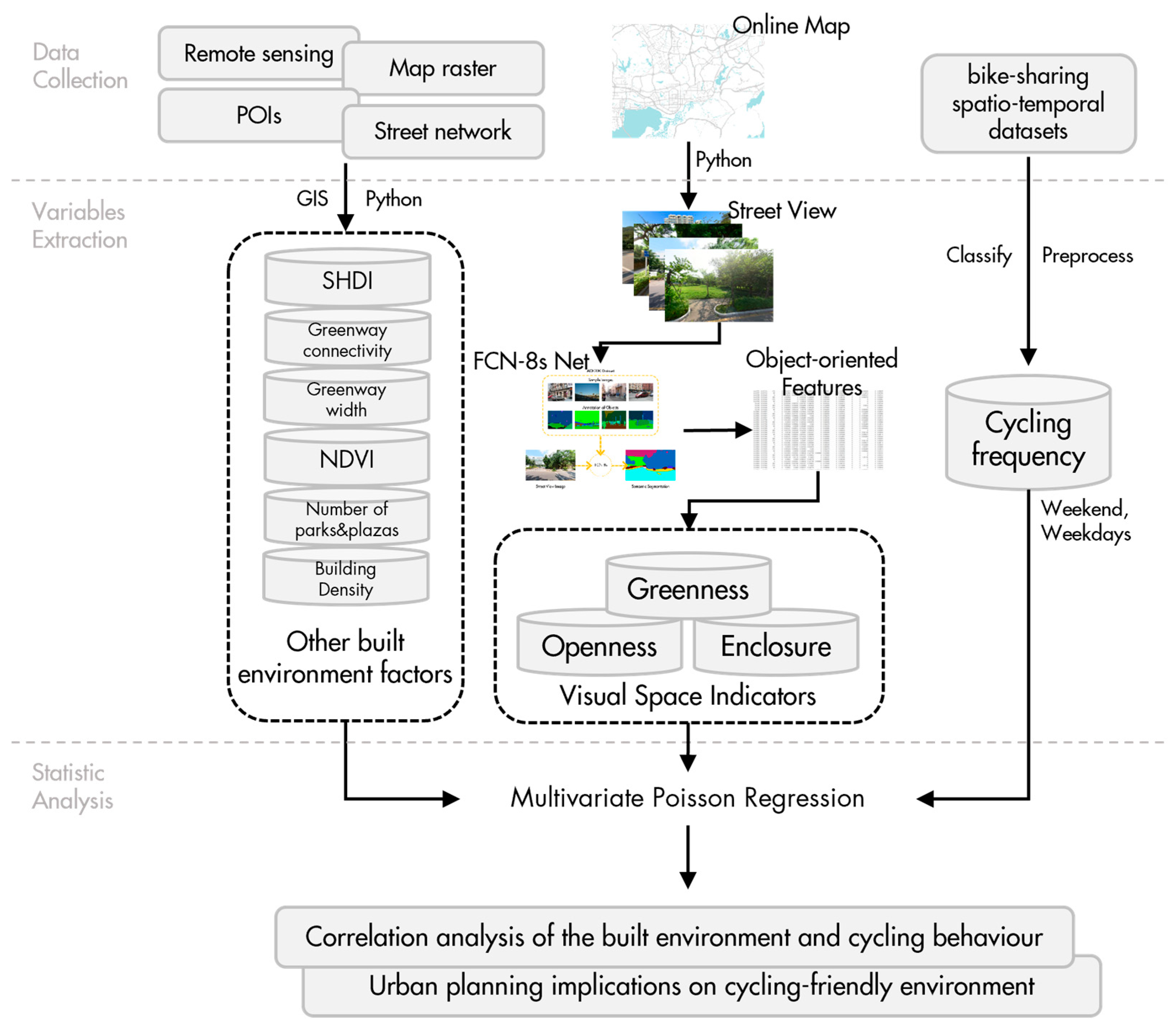
2. Materials and Methods

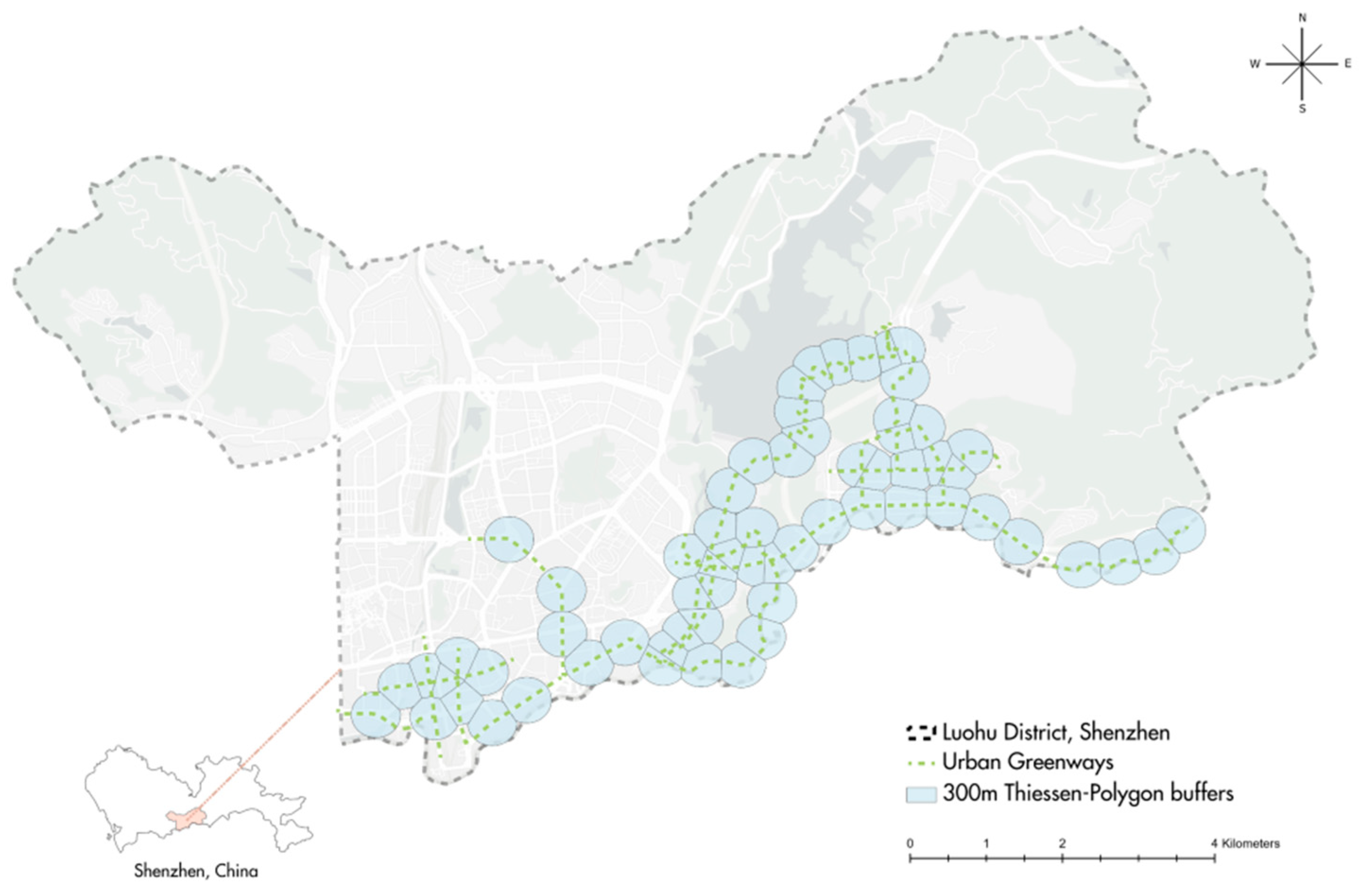
2.1. Study Area

Shenzhen is one of the major cities in southern China, located in the Pearl River Delta, close to Hong Kong, with a high population density and vibrant economic activity. It has a stable bicycle-sharing service in place, making it a popular choice for researchers from various fields [20,22,87,92]. Based on data from October 2018, the average daily usage of shared bicycles in Shenzhen reached 650,000 [87]. Additionally, the area covered by greenways in Shenzhen is one of the longest in China. According to data from 2015, Shenzhen’s greenway network comprises 342 km of regional greenways, 673 km of urban greenways, and 1031 km of community greenways [93].

Greenways serve multiple purposes including beautification, recreation, and the fulfilment of ecological and diverse human needs [94]. The Pearl River Delta (PRD) Greenway Network is the first modern greenway project to be implemented in China [95], which seeks to improve the ecological environment, raise the standard of living, and drive economic growth, and as a result of this programme, 18,019 km of greenways had been built in Guangdong Province by the end of 2018 [96]. Although the programme has provided some public facilities and boosted the tourism economy in less-developed villages, the ecological and human functions of the greenways have been overlooked in the rush to achieve results. It has been noted that there is a lack of expertise in greenway planning and implementation of this greenway network as well as sound ecological and landscaping strategies [91]. Forming part of this greenway network, most of Shenzhen’s greenways are situated in built-up areas, and from our observations, many of them often overlap with transportation corridors and have narrow widths and limited ecological functions, rendering them impractical for outdoor sports and cycling. This situation is not only the result of land resource constraints but also the fact that current greenway planning places excessive emphasis on the transportation function of the greenway network and fails to consider the needs of non-motorised transport. To address this dilemma, this study aims to investigate the relationship between the greenway environment and cycling behaviour through quantitative analysis, with the objective of offering theoretical support for future greenway planning in highly populated areas.

Based on greenway data from the Shenzhen government’s open data platform, this study selected 23 urban greenways in the Luohu District after excluding those with incomplete data or bicycle-access bans. Consequently, the creation of buffers around the greenways was required to investigate the impact of the built environment on cycling behaviour at a spatial scale. To avoid overlapping buffers and double-counting of cycling activity, we used the Thiessen-polygon method to ensure that they were all independent [22,97,98]. The sampling points were generated along the path of each urban greenway on a 500 m scale, and buffer zones of 300 m were created using ArcGIS Pro software based on the greenway sampling points (Figure 1).

2.2. Variables

2.2.1. Cycling Frequency

Following previous studies [20,22,99], the number of bike-sharing trips was chosen as the dependent variable in this study. We investigated cycling behaviour along the greenways and trips that began or finished within the buffer zone. In this study, dockless bicycle sharing data were obtained from the daily order dataset of bicycle-sharing companies updated by the Shenzhen government’s open data platform (https://opendata.sz.gov.cn/data/dataSet/toDataDetails/29200_00403627, accessed on 13 August 2022). The dataset provides data on bicycle sharing in Shenzhen in 2020 and 2021, which is anonymised and contains user and company IDs, latitude and longitude coordinates of the start and end points of journeys, and timestamps. This paper selected six days of rides from 6 to 11 April 2021, a period that included four weekdays and one weekend, during which the dataset recorded approximately two million rides within Shenzhen. The meteorological conditions during the given period were conducive to cycling, characterised by sunny skies and temperatures ranging from 21 °C to 29 °C.

The steps involved in processing the data were as follows. First, greenways possess not only recreational attributes but also serve as transport corridors for accessing other destinations [47]. This dual function raises the possibility that people may use them primarily for transportation rather than for their environmental qualities. To mitigate the impact of mobility purposes on cycling behaviour, this study only selected cycling data with departure times between 10 a.m. and 3 p.m. Second, it was necessary to exclude travel data unrelated to actual cycling behaviour [17,87,100]. Therefore, data that were too short in duration (less than 3 min) and too fast in speed (greater than 20 km/h) were also excluded. These anomalies may result from redeployment by the bike-sharing company and data input errors. The speed was calculated based on the straight-line distance and duration of the trip. The distance was calculated by importing each trip’s start and end coordinates into GIS software. As the dataset does not record the actual route of each trip, it was not possible to identify the precise distance travelled. Thirdly, only bicycle trips starting or ending in the buffer zone were considered. This produced a final total of 139,018 trips within the buffer zone. After cleaning and filtering the raw data, the cycling data were further categorised into weekdays and weekends to examine the impact of any potential temporal differences on cycling behaviour.

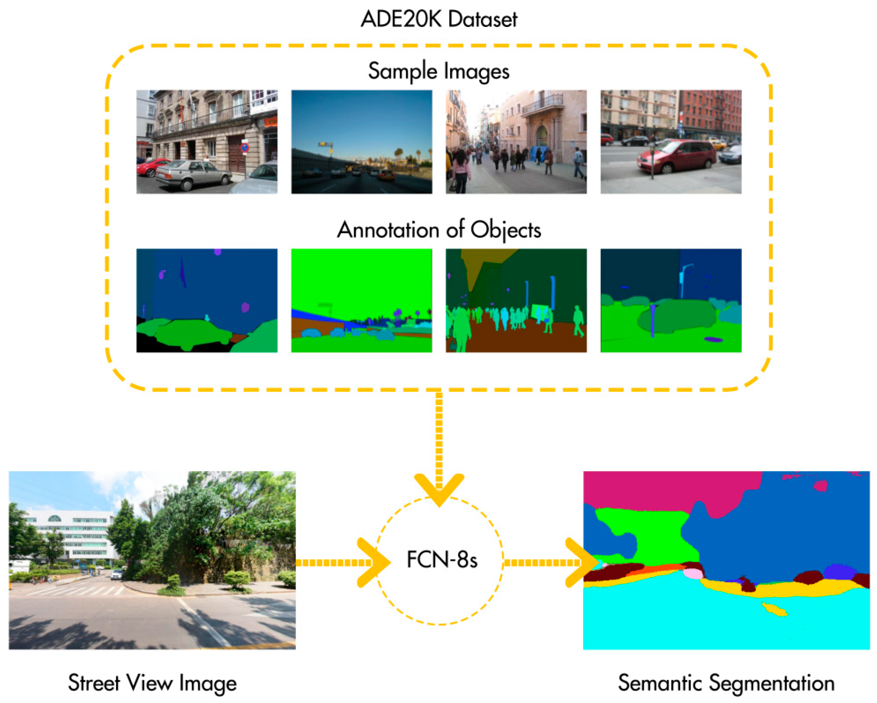
2.2.2. Visual Space Indicators

This study used street-view images from Baidu Maps with streetscape recognition techniques to measure the built environment. Baidu Street View (BSV) is the main source of street-view data in China and has been employed in many studies [64,101,102]. The BSV is a 360-degree horizontal and 180-degree vertical panoramic image and can be accessed online. Based on OpenStreetMap (OSM) data [103], 5242 street-view sampling points were generated along each street at a sampling distance of 100 m. Each sampling point’s latitude and longitude coordinates were then recorded, and the street-view images were taken in four directions: 0, 90, 180, and 270 degrees [20,104,105]. The size of each street view image was 480 × 320 pixels, and the vertical angle was 0 degrees. A final total of 14,947 street images was obtained.

Deep learning methods are able to extract high-dimensional visual features to enhance the understanding of images [1,106]. Moreover, semantic segmentation models can detect the proportion of different types of objects in street-view images [58,73,107]. Therefore, they have become the primary tool used for streetscape processing in the built environment field [52]. This study used a visual image semantic segmentation program [62] and trained the fully convolutional network (FCN) using the ADE20K dataset [108]. FCNs have been shown to successfully identify everyday objects in street-view images and predict their semantic properties [53,58]. The pixel comparison accuracy of the network was 0.814426 and 0.66839 for the training and test datasets, respectively. The street-view image data acquired were then processed by this trained segmentation model (Figure 2).

In this study, three different visual space indicators from a human perspective were selected as independent variables in order to analyse their relationship with cycling behaviour, namely openness, greenness, and enclosure. In the process of street-view data acquisition described above, four images were collected for each sampling point, with azimuth angles of 0, 90, 180, and 270. The number of pixels accounted for by the visual elements, such as greenery, sky, and buildings, was then calculated using the FCN-based segmentation method, and the proportion of the whole scene that they occupied was determined. The greenness of each sample point was calculated by the ratio of the number of pixels in the trees and plants in each image to the total number of pixels in each image using the following formula:

$$Greennes{s}_{sample}=\frac{{{\displaystyle \sum }}_{i=1}^{4}pixel{s}_{t\_i}+{{\displaystyle \sum }}_{i=1}^{4}pixel{s}_{p\_i}}{{{\displaystyle \sum }}_{i=1}^{4}pixel{s}_{o\_i}}$$

(1)

In Equation (1), $pixel{s}_{t\_i}$ denotes the number of pixels in trees segmented from photos taken in the ith direction of each sampling point in the four directions, $pixel{s}_{p\_i}$ denotes the number of pixels in plants segmented from streetscape images in the ith direction, and $pixel{s}_{o\_i}$ denotes the total number of pixels in streetscape images in the ith direction. Based on Equation (1), Equation (2) was formulated to quantify the greenness of the study area, where n denotes the number of sampling points in each buffer, and $Greennes{s}_{sample}$ denotes the value of the greenness index of each sampling point.

$$Greennes{s}_{site}=\frac{{{\displaystyle \sum }}_{j=1}^{n}Greennes{s}_{sample}{}_j}{n}\times 100\%$$

(2)

Openness represents the portion of the sky visible from the ground. This study uses sky exposure to reflect openness. The openness was calculated by the ratio of the number of pixels in the sky to the total number of pixels in the street-view images. Equation (3) was used to quantify the openness of each sampling point, and Equation (4) was used to quantify the openness within the study area as a whole. $pixel{s}_{s\_i}$ denotes the number of sky pixels extracted from the picture taken in the ith direction at each sampling point, and $Opennes{s}_{sample}$ denotes the openness index calculated for each sampling point.

$$Opennes{s}_{sample}=\frac{{{\displaystyle \sum }}_{i=1}^{4}pixel{s}_{s\_i}}{{{\displaystyle \sum }}_{i=1}^{4}pixel{s}_{o\_i}}$$

(3)

$$Opennes{s}_{site}=\frac{{{\displaystyle \sum }}_{j=1}^{n}Opennes{s}_{sample}{}_j}{n}\times 100\%$$

(4)

Enclosure refers to the extent to which people are spatially enclosed by the urban environment. Following previous studies [82], the enclosure was calculated by the ratio of the number of pixels in trees and buildings to the total number of pixels in the street view image. Equation (5) was used to quantify the enclosure of each sampling point, while Equation (6) was used to quantify the enclosure within the study area overall. $pixel{s}_{b\_i}$ represents the number of pixels in the buildings extracted from the photograph taken in the ith direction at each sample point, and $Enclosur{e}_{sample}$ represents the value of enclosure calculated at each sample point. A higher enclosure value means a denser spatial enclosure.

$$Enclosur{e}_{sample}=\frac{{{\displaystyle \sum }}_{i=1}^{4}pixel{s}_{t\_i}+{{\displaystyle \sum }}_{i=1}^{4}pixel{s}_{b\_i}}{{{\displaystyle \sum }}_{i=1}^{4}pixel{s}_{o\_i}}$$

(5)

$$Enclosur{e}_{site}=\frac{{{\displaystyle \sum }}_{j=1}^{n}Enclosur{e}_{sample}{}_j}{n}\times 100\%$$

(6)

2.2.3. Covariables

Developing the work of previous studies [10,21,22] further, this study considered the built environment characteristics that may affect cycling behaviour. These factors include the normalised difference vegetation index (NDVI), land-use mix, the greenway link-node ratio, building density, number of parks and plazas, and greenway width.

The normalised difference vegetation index (NDVI) is an indicator used to assess vegetation exposure at a large scale from a vertical perspective. The NDVI is calculated based on the contrast between the two bands (chlorophyll pigment absorption in the red band and high reflectance of plant material in the near-infrared band) through remote sensing image data [10]. The remote sensing data were obtained from Landsat 8 OLI_TIRS satellite digital products provided by Geospatial Data Cloud (http://www.gscloud.cn/sources/accessdata/411?pid=1, accessed on 13 August 2022), with an image resolution of 30 m, taken on 20 February 2021, with cloudiness of 0.04%. The raster of the remote sensing images was imported using GIS software, and the NDVI was calculated, followed by the average NDVI value of each buffer zone. The higher values represent greater amounts of vegetation in the area. The equation used to calculate NDVI is as follows, in which NIR denotes the near-infrared band, and R refers to the red band:

$$NDVI=\frac{NIR-R}{NIR+R}$$

(7)

The land-use mix was calculated using 14 different types of point of interest (POI) data, and the relative percentages of different land-use types were ascertained [109]. The number and type of POI in each buffer with a search radius of 100 m were then calculated using ArcGIS software. Subsequently, the proportion of each type in each buffer was calculated to arrive at a measure of the land-use mix, also known as the Shannon–Wiener diversity index (SHDI) [110]. The equation for calculating SHDI is as follows:

$$SHDI=-{\displaystyle \sum }_{i=1}^m{p}_i\times \ln p_i$$

(8)

where $p_i$ is the proportion of type i in the whole buffer, and m is the total number of types of POI in the buffer. This indicator is greatest when there is a similar proportion of POIs of each type. When there is only one type of POI or none at all in the area, the value is zero. Land-use mix is a measure of the functional complexity of an area and has been widely used in research on the built environment [17,21,72,111]. Compact, mixed-use urban environments have been shown to promote cycling [31,34].

We also included four other indicators: link-node ratio, building density, number of parks and plazas, and greenway width. First, the link-node ratio refers to the connectivity of the greenway to the surrounding roads. The link-node ratio was obtained by dividing the number of links by the number of nodes on the greenway. Links are greenway segments, and nodes are greenway intersections or cul-de-sacs. Higher ratio values indicate better connectivity. Second, building density is defined as the ratio of the area covered by buildings within a buffer to the buffer area as a whole. A higher ratio indicates a more densely built-up area, reflecting a more densely populated area with more traffic activity. Third, the number of parks and plazas was calculated from the number of parks and plaza POIs in the buffer zone. Fourth, greenway width is the average width of greenways in the buffer zone.

2.3. Statistical Analysis

Following previous studies [22,99], as cycling frequency is a count variable, this study used a multivariate Poisson regression model to investigate the influence of visual-spatial factors on cycling behaviour along greenways. Each of the three visual space indicators was used as the independent variable in the regression model. The variance inflation factor (VIF) of each variable was less than 5 in the multi-collinearity test, so it was concluded that there was no significant collinearity in the model in this study. The model used in this study was specified as follows:

$$P\left(Y=y_i|\lambda \right)=\frac{{\lambda }^{{\beta }_0+{\beta }_1{V}_i+{\beta }_2{C}_i+{\epsilon }_i}{e}^{-\lambda }}{({\beta }_0+{\beta }_1{V}_i+{\beta }_2{C}_i+{\epsilon }_i)!}$$

(9)

where $y_i$ represents the use of bicycle sharing around the greenway, $V_i$ denotes a vector of variables of the three visual spatial indicators, $C_i$ denotes a vector of covariates, λ denotes the Poisson event rate, and ${\epsilon }_i$ denotes the random error.

Previous studies [83,99] have shown that cycling behaviour may differ across periods of time. Therefore, this study used two regression models to examine cycling behaviour on weekdays and at weekends and their relationship with the built environment consisting of urban greenways.

Figure 3 presents the flowchart of this study. Firstly, the study initially collected data from various sources, including street-view images, bicycle-sharing data, remote sensing images, and map data. Secondly, each street view-image underwent semantic segmentation using the FCN-8 s model, which enabled us to obtain the proportion of different objects and calculate three visual spatial indicators. GIS and python were also used to process the data and extract the cycling frequency on weekends and weekdays along with other built environment factors. Thirdly, a multivariate Poisson regression analysis was conducted to investigate the association between cycling and the built environment, suggesting implications for promoting bicycle-friendly environments and greenway planning.

3. Results

3.1. Descriptive Analysis

Table 1. Descriptive statistics.

	Variables	Mean (SD)
Dependent variables	Cycling frequency at weekends (total number of rides)	1200.625 (1688.951)
	Cycling frequency on weekdays (total number of rides)	971.531 (1526.465)
Visual space indicators	Greenness (%)	26.494 (15.548)
	Openness (%)	13.117 (4.956)
	Enclosure (%)	37.348 (9.342)
Covariates	NDVI (%)	14.675 (6.785)
	Land-use mix (SHDI)	1.801 (0.659)
	Greenway connectivity (link-node ratio)	1.327 (0.611)
	Greenway width (m)	2.524 (0.657)
	Building density (km2/km2)	0.161 (0.123)
	Number of parks and plazas (number)	1.375 (2.616)

SD, standard deviation.

summarises the properties of all the variables. The average number of rides in the study area varies by time period, with weekends seeing a higher number of rides than weekdays. The average number of rides at weekends was 1200.625 compared to 971.531 on weekdays, indicating that cycling is more frequent on weekends. In terms of visual space indicators, the study area is generally quite enclosed, with an average greenness rating of 26.494, an average openness value of 13.117, and an average enclosure value of 37.348.

With regard to the covariates, the mean NDVI of the study area was 14.675, which was generally lower than the visual-spatial indicator of greenness, suggesting that the vertical perspective measurement may be different from the actual greenness observed by the human eye. The average land-use mix of the study area was 1.801, the average greenway link-node ratio was 1.327, the average greenway width was 2.524, the average building density was 0.161, and the average number of parks and squares was 1.375.

3.2. Baseline Results

Table 2. The regression model results with regard to street-view greenness.

	Cycling Frequency at Weekend	Cycling Frequency on Weekdays	Cycling Frequency in a Week
	Coef. (SE)	Coef. (SE)	Coef. (SE)
Visual space indicators
Greenness	0.015 *** (0.001)	0.014 *** (0.001)	0.015 *** (0.001)
Covariates
NDVI	−0.184 *** (0.001)	−0.211 *** (0.002)	−0.196 *** (0.001)
Land-use mix	1.881 *** (0.025)	2.175 *** (0.035)	1.967 *** (0.020)
Greenway connectivity	−0.379 *** (0.011)	−0.566 *** (0.013)	−0.456 *** (0.008)
Greenway width	0.330 *** (0.012)	0.062 *** (0.015)	0.224 *** (0.009)
Building density	1.185 *** (0.054)	1.395 *** (0.062)	1.228 *** (0.041)
Number of parks and plazas	0.027 *** (0.001)	0.032 *** (0.001)	0.029 *** (0.001)

Coef., coefficient; SE, standard error; *** p < 0.01.

shows the effect of visually perceived greenery and built environment characteristics on cycling behaviour along the urban greenway on weekends and on weekdays. The results show that greenness is positively associated with cycling behaviour during different periods of time. In contrast, NDVI was negatively correlated with cycling behaviour. Land-use mix, greenway width, building density, and the number of parks and plazas were all positively associated with cycling behaviour. However, greenway connectivity was negatively correlated with cycling behaviour.

Table 3. The regression model results with regard to street-view openness.

	Cycling Frequency at Weekend	Cycling Frequency on Weekdays	Cycling Frequency in a Week
	Coef. (SE)	Coef. (SE)	Coef. (SE)
Visual space indicators
Openness	0.005 *** (0.001)	−0.011 *** (0.001)	−0.003 ** (0.001)
Covariates
NDVI	−0.169 *** (0.001)	−0.192 *** (0.001)	−0.179 *** (0.001)
Land-use mix	1.620 *** (0.022)	1.996 *** (0.032)	1.747 *** (0.018)
Greenway connectivity	−0.342 *** (0.010)	−0.531 *** (0.012)	−0.419 *** (0.008)
Greenway width	0.349 *** (0.012)	0.109 *** (0.016)	0.255 *** (0.010)
Building density	1.311 *** (0.057)	1.203 *** (0.066)	1.199 *** (0.043)
Number of parks and plazas	0.033 *** (0.001)	0.037 *** (0.001)	0.034 *** (0.001)

Coef., coefficient; SE, standard error; ** p < 0.05; *** p < 0.01.

shows the effect of visually perceived sky openness and built environment characteristics on cycling behaviour along the urban greenway om weekends and on weekdays. The regression results show that openness is positively correlated with cycling behaviour on weekends but negatively correlated with cycling behaviour on weekdays. In terms of the covariates, the regression results in Table 3 are similar to those in Table 2, with land-use mix, greenway width, building density, and number of parks and plazas all positively associated with cycling behaviour and NDVI and greenway connectivity negatively correlated with cycling behaviour on weekends and on weekdays.

Table 4. The regression model results with regard to street-view enclosure.

	Cycling Frequency at Weekend	Cycling Frequency on Weekdays	Cycling Frequency in a Week
	Coef. (SE)	Coef. (SE)	Coef. (SE)
Visual space indicators
Enclosure	0.016 *** (0.001)	0.016 *** (0.001)	0.017 *** (0.001)
Covariates
NDVI	−0.163 *** (0.001)	−0.190 *** (0.001)	−0.175 *** (0.001)
Land-use mix	1.806 *** (0.024)	2.098 *** (0.033)	1.898 *** (0.019)
Greenway connectivity	−0.343 *** (0.01)	−0.527 *** (0.012)	−0.417 *** (0.008)
Greenway width	0.377 *** (0.012)	0.109 *** (0.016)	0.273 *** (0.009)
Building density	0.696 *** (0.063)	0.857 *** (0.072)	0.689 *** (0.047)
Number of parks and plazas	0.030 *** (0.001)	0.034 *** (0.001)	0.032 *** (0.001)

Coef., coefficient; SE, standard error; *** p < 0.01.

illustrates the effect of visual enclosure and built environment characteristics on cycling behaviour around the urban greenway on weekends and on weekdays. The results show that enclosure was positively associated with cycling behaviour. In terms of the covariates, the regression results in Table 4 are similar to those in Table 2. Land-use mix, greenway width, building density, and the number of parks and plazas were all positively correlated with cycling behaviour at different times, while NDVI and greenway connectivity were negatively related to cycling behaviour on weekends and on weekdays.

4. Discussion

4.1. The Association between Visual Space and Cycling Behaviour

In this paper, our results suggest that the greenness and enclosure of the greenway were positively associated with cycling behaviour on weekdays and the weekend. The openness of the sky within the greenway environment had a positive effect on cycling during the weekend but a negative influence during the weekdays.

The positive correlation between greenness and cycling behaviour can be explained by the fact that greenness provides a pleasant and comfortable cycling environment. On the one hand, the presence of urban greenery has an emotional and/or psychological value. Greenery can improve the aesthetic perception of the built environment [10,112]. It has been shown that residents give higher aesthetic ratings to urban environments containing more trees [113]. Moreover, greenness can also enhance mental health and improve the mood of urban residents [44,70]. Numerous studies have observed a positive correlation between psychological well-being and visible greenery [82,104,105]. In addition, greenness provides a pleasant environment and can reduce air pollution. The combined effect of shade and evapotranspiration from trees has been shown to reduce surface air temperatures in urban areas and decrease the effects of “urban heat islands” [114,115]. Street trees can therefore provide a safer, more thermally comfortable travel environment [114,116]. Not only that, but greenness also plays a role in reducing air pollution. Urban street trees can absorb air pollution and improve walkability [58]. Wu et al. [73] found that an increase in vertically distributed street greenery was effective at reducing air pollution in streets in the summertime.

In this paper, it was discovered that greater enclosure of visual space could promote cycling behaviour. This is because well-enclosed spaces tend to provide a higher level of safety and thus encourage more physical activity [117,118]. An enclosed street gives the impression of safety [82,117], whereas a broad structure creates a sense of vacancy and inactivity [53,119,120]. A study by Ma et al. [121] found that as central urban areas tend to be more enclosed, residents in urban centres had a greater sense of safety [122]. Moreover, a greater level of enclosure can also provide a more thermally comfortable urban environment. Because trees and buildings intercept solar radiation and cast shadows, they may affect the microclimate and the physiological equivalent temperature (PET) [123]. A low level of sky visibility and dense green cover have been shown to reduce the PET at ground level [124].

The results of this study further suggested that people prefer a larger area of sky for cycling during weekends, while they favour a smaller area of sky openness during weekdays. This may be due to differences in the purpose of their cycle rides. On the one hand, people prefer to cycle for recreational activities on weekends [22,83], when they are more concerned with visual perception and the cycling experience. The openness of streets has been shown to increase the attractiveness of streetscapes and enhance people’s comfort at public events [53]. This phenomenon can be explained by the fact that sunny weather increases serotonin levels, the brain’s happiness-enhancing neurotransmitters, thereby improving mood [125], for example, by reducing sadness [126], tiredness, and sluggishness [127] and increasing optimism and concentration [128]. It has been found that the number of cyclists increases threefold in summer compared to winter [129]. A study by Böcker et al. [130] in the Netherlands also showed that dry, calm, sunny, and warm but not-too-hot (up to 25 °C) weather enhances positive effects such as happiness and enthusiasm and therefore promotes cycling behaviour. On the other hand, when people cycle mainly for weekday commuting [131], they are more concerned with cycling efficiency and comfort. Cyclists are more likely to be exposed to current weather conditions [132] and are therefore more sensitive to climate. Hot weather not only affects human comfort and health but also inhibits mood and active travel [123]. In a study set in Singapore, Meng et al. [5] found that cycling behaviour was more likely to occur in scenarios where temperatures were relatively low. Higher air temperatures may not be conductive to cycling [17,130,133].

4.2. Other Built Environment Factors

The results of this study suggest that NDVI and the actual amount of greenery perceived within a visual space do not have a consistent influence on cycling behaviour. There may be two reasons for this phenomenon. On the one hand, NDVI and visual greenery are observed from different perspectives. NDVI, which is calculated from remote sensing images taken by satellites from high altitudes, may not accurately represent the presence of vegetation that is obscured by tree canopies or structures such as overpasses or buildings. In contrast, street-view images, which provide a ground-level perspective, can accurately measure greenery that is perceived within the actual environment [134]. On the other hand, they also use different scopes of measurement. Whereas visual greenness calculated from street-view images focuses on road greenness, NDVI measures the vegetation cover of a whole site, such as a park, farmland, hill, etc. However, not all places are suitable for cycling. Cycling usually occurs on streets or cycle paths [10,22]. As a result, cycling behaviour is more likely to be affected by visual greenness than by NDVI.

Our findings show that land-use mix, greenway width, building density, and the number of parks and plazas are all positively associated with cycling behaviour. This is because areas with a high land-use mix have more urban functions and a variety of travel purposes and are thus likely to promote cycling behaviour [17,92]. Moreover, wider greenways offer a better natural environment to support physical activity [21], and the role of urban parks in promoting physical activity has been confirmed by several studies [112,135]. In addition, greater building density is associated with higher activity levels [72,136] and therefore promotes physical activity [99,137]. However, greenway connectivity was negatively associated with cycling behaviour. This may be because the complexity of traffic activity around intersections may be detrimental to cycling safety. It has been noted that cyclists are more likely to use cycle lanes if they do not need to cross busy streets [138].

4.3. Implications for Urban Design and Planning

As a study designed to examine the effects of urban greenways within the built environment, the findings may provide some insights into the planning and construction of future greenways. Firstly, the visual greenness and enclosure of spaces are likely to have a positive relationship with cycling behaviour, and the number of parks and plazas in an area may also promote cycling. To create environmentally sustainable, bicycle-friendly cities and to further promote active travel behaviour such as cycling, urban planners and designers need to improve the quality, not just the quantity, of green space within greenways. An Australian study reported that the quality rather than the quantity of community green space improved residents’ psychological well-being [139]. Lu [112] also found that the quality of street greenery can promote physical activity. Therefore, not only is it necessary to build more greenways and parks, but there is also a need for high-quality, tree-lined cycling environments. Examples include increasing the diversity of plants, adding vertical greenery [140], and planting more lush trees.

Secondly, the relationship between sky openness and cycling behaviour is influenced by weather conditions and subjective emotions, and people generally prefer sunny but not-too-hot weather. Therefore, designers should consider how to increase sunlight and reduce the perceived temperature of an environment. On the one hand, policies such as tree planting to increase shade cover can improve thermal conditions to encourage active travel [123]; on the other hand, increasing the greenway width not only promotes cycling but also increases the sunlit area of the greenway in general, thus improving the overall brightness of the environment by creating more light reflectivity.

Last but not least, this study shows that high levels of greenway connectivity inhibit cycling behaviour. This may be because areas with complex traffic conditions can decrease cycling safety. Due to concerns about traffic safety, the lack of a good cycle path system may limit cycling activity [10]. This highlights the need for planners and designers to create more systematic and safe cycle paths [141]. Urban planners could improve cycling conditions by increasing the number of routes and lanes and by linking large green spaces, parks and squares, and other cycling infrastructure together to develop a network of cycle paths.

4.4. Strengths and Limitations

This study has several strengths. Firstly, we utilised bike-sharing location data to measure cycling behaviour by calculating the number of bicycle trips made within the study area, while the extensive sample size ensured the reliability of the findings. Secondly, in addition to analysing visual greenery using street-view image data, the study also considered two visual indicators: openness and enclosure, which allowed for a more nuanced understanding of the built environment at a human scale. Thirdly, we further compared the relationship between cycling behaviour and the built environment consisting of urban greenways during different periods (weekdays and weekends) using the bike-sharing data, which included both location information and the start and end times of each trip.

Although street-view images can provide a fresh perspective on the built environment, they still have some limitations. Firstly, the time at which the street-view images are captured is inconsistent. BSV data are not taken at the same time every day, making it challenging to analyse the urban environment over a fixed period. However, greenery and buildings vary gradually, and as the study area is located in southern China, the subtropical climate means that most vegetation is evergreen or semi-evergreen. Therefore, the measurement of visual space indicators is still reliable. Secondly, the street-view images may not fully simulate the human perspective while riding a bicycle. BSVs are mainly taken by car and, only in a few cases, by bicycle. This means that BSVs are mainly captured on motorways rather than cycle lanes or side roads. Although BSV captures a 360° view of the surrounding area, the perspective of cars and bicycles differs slightly and may thus result in different perceptions of the urban environment. Thirdly, for data availability reasons, demographic and socio-economic information, cycling purpose, and individual cycling data were not included in this study. Furthermore, as the cycling data do not contain user travel routes, it is not possible to accurately measure bike traffic and the built environment characteristics of the journey just from the start and end points. Finally, despite selecting travel times and locations to avoid the influence of other demands on cycling behaviour, we are unable to entirely measure cycling behaviour that is solely affected by the greenway environment.

5. Conclusions

In this study, we investigated the association between the built environment, particularly greenways, and cycling behaviour from a human-scale perspective. By analysing bike-sharing data and streetscape image data using machine learning techniques and a multivariate Poisson regression model, the study found that greenness and enclosure of greenways are positively associated with cycling behaviour, with openness promoting cycling on weekends but having the opposite effect on weekdays. The study also revealed that satellite-based measurements of urban greenery, such as NDVI, may not reflect human-scale perceptions effectively. The findings have important implications for policymakers and urban planners seeking to promote green transportation and bicycle-friendly cities. They need to consider the visual space of the cycling environment and improve its comfort and safety. Additionally, our study highlights the potential of street-view data in further research on the relationship between urban perceptions, sustainable cities, and transport. Nevertheless, our study’s limits need to be acknowledged. The inability to track user travel routes and the potential influence of external factors limit the accuracy of measuring bike traffic and the impact of the built environment on cycling behaviour. Therefore, further research is necessary to expand our understanding of the complex interactions.

References

1. Kang, Y.; Zhang, F.; Gao, S.; Lin, H.; Liu, Y. A Review of Urban Physical Environment Sensing Using Street View Imagery in Public Health Studies. Ann. GIS 2020, 26, 261–275. [Google Scholar] [CrossRef]
2. United Nations World Urbanization Prospects 2018—World’s Largest Cities. Available online: https://www.un.org/en/desa/world-urbanization-prospects-2018-worlds-largest-cities (accessed on 24 August 2022).
3. Eren, E.; Uz, V.E. A Review on Bike-Sharing: The Factors Affecting Bike-Sharing Demand. Sustain. Cities Soc. 2020, 54, 101882. [Google Scholar] [CrossRef]
4. Zhao, J.; Wang, J.; Deng, W. Exploring Bikesharing Travel Time and Trip Chain by Gender and Day of the Week. Transp. Res. Part C Emerg. Technol. 2015, 58, 251–264. [Google Scholar] [CrossRef]
5. Meng, M.; Zhang, J.; Wong, Y.D.; Au, P.H. Effect of Weather Conditions and Weather Forecast on Cycling Travel Behavior in Singapore. Int. J. Sustain. Transp. 2016, 10, 773–780. [Google Scholar] [CrossRef]
6. El-Assi, W.; Salah Mahmoud, M.; Nurul Habib, K. Effects of Built Environment and Weather on Bike Sharing Demand: A Station Level Analysis of Commercial Bike Sharing in Toronto. Transportation 2017, 44, 589–613. [Google Scholar] [CrossRef]
7. Xu, Y.; Chen, D.; Zhang, X.; Tu, W.; Chen, Y.; Shen, Y.; Ratti, C. Unravel the Landscape and Pulses of Cycling Activities from a Dockless Bike-Sharing System. Comput. Environ. Urban Syst. 2019, 75, 184–203. [Google Scholar] [CrossRef]
8. Cheng, L.; Yang, J.; Chen, X.; Cao, M.; Zhou, H.; Sun, Y. How Could the Station-Based Bike Sharing System and the Free-Floating Bike Sharing System Be Coordinated? J. Transp. Geogr. 2020, 89, 102896. [Google Scholar] [CrossRef]
9. Chen, P.; Zhou, J.; Sun, F. Built Environment Determinants of Bicycle Volume: A Longitudinal Analysis. J. Transp. Land Use 2017, 10, 655–674. [Google Scholar] [CrossRef] [Green Version]
10. Lu, Y.; Yang, Y.; Sun, G.; Gou, Z. Associations between Overhead-View and Eye-Level Urban Greenness and Cycling Behaviors. Cities 2019, 88, 10–18. [Google Scholar] [CrossRef]
11. Wang, Y.; Chau, C.K.; Ng, W.Y.; Leung, T.M. A Review on the Effects of Physical Built Environment Attributes on Enhancing Walking and Cycling Activity Levels within Residential Neighborhoods. Cities 2016, 50, 1–15. [Google Scholar] [CrossRef]
12. Yang, Y.; Wu, X.; Zhou, P.; Gou, Z.; Lu, Y. Towards a Cycling-Friendly City: An Updated Review of the Associations between Built Environment and Cycling Behaviors (2007–2017). J. Transp. Health 2019, 14, 100613. [Google Scholar] [CrossRef]
13. Wu, X.; Lu, Y.; Gong, Y.; Kang, Y.; Yang, L.; Gou, Z. The Impacts of the Built Environment on Bicycle-Metro Transfer Trips: A New Method to Delineate Metro Catchment Area Based on People’s Actual Cycling Space. J. Transp. Geogr. 2021, 97, 103215. [Google Scholar] [CrossRef]
14. Chen, W.; Chen, X.; Chen, J.; Cheng, L. What Factors Influence Ridership of Station-Based Bike Sharing and Free-Floating Bike Sharing at Rail Transit Stations? Int. J. Sustain. Transp. 2022, 16, 357–373. [Google Scholar] [CrossRef]
15. Cheng, L.; Wang, K.; De Vos, J.; Huang, J.; Witlox, F. Exploring Non-Linear Built Environment Effects on the Integration of Free-Floating Bike-Share and Urban Rail Transport: A Quantile Regression Approach. Transp. Res. Part A Policy Pract. 2022, 162, 175–187. [Google Scholar] [CrossRef]
16. Ospina, J.P.; Duque, J.C.; Botero-Fernández, V.; Brussel, M. Understanding the Effect of Sociodemographic, Natural and Built Environment Factors on Cycling Accessibility. J. Transp. Geogr. 2022, 102, 103386. [Google Scholar] [CrossRef]
17. Shen, Y.; Zhang, X.; Zhao, J. Understanding the Usage of Dockless Bike Sharing in Singapore. Int. J. Sustain. Transp. 2018, 12, 686–700. [Google Scholar] [CrossRef]
18. Lanzendorf, M.; Busch-Geertsema, A. The Cycling Boom in Large German Cities—Empirical Evidence for Successful Cycling Campaigns. Transp. Policy 2014, 36, 26–33. [Google Scholar] [CrossRef]
19. Pucher, J.; Buehler, R.; Seinen, M. Bicycling Renaissance in North America? An Update and Re-Appraisal of Cycling Trends and Policies. Transp. Res. Part A Policy Pract. 2011, 45, 451–475. [Google Scholar] [CrossRef]
20. Chen, Y.; Chen, Y.; Tu, W.; Zeng, X. Is Eye-Level Greening Associated with the Use of Dockless Shared Bicycles? Urban For. Urban Green. 2020, 51, 126690. [Google Scholar] [CrossRef]
21. Liu, K.; Siu, K.W.M.; Gong, X.Y.; Gao, Y.; Lu, D. Where Do Networks Really Work? The Effects of the Shenzhen Greenway Network on Supporting Physical Activities. Landsc. Urban Plan. 2016, 152, 49–58. [Google Scholar] [CrossRef] [Green Version]
22. Wang, R.; Lu, Y.; Wu, X.; Liu, Y.; Yao, Y. Relationship between Eye-Level Greenness and Cycling Frequency around Metro Stations in Shenzhen, China: A Big Data Approach. Sustain. Cities Soc. 2020, 59, 102201. [Google Scholar] [CrossRef]
23. Cole-Hunter, T.; Donaire-Gonzalez, D.; Curto, A.; Ambros, A.; Valentin, A.; Garcia-Aymerich, J.; Martínez, D.; Braun, L.M.; Mendez, M.; Jerrett, M.; et al. Objective Correlates and Determinants of Bicycle Commuting Propensity in an Urban Environment. Transp. Res. Part D Transp. Environ. 2015, 40, 132–143. [Google Scholar] [CrossRef]
24. Calogiuri, G.; Elliott, L.R. Why Do People Exercise in Natural Environments? Norwegian Adults’ Motives for Nature-, Gym-, and Sports-Based Exercise. Int. J. Environ. Res. Public Health 2017, 14, 377. [Google Scholar] [CrossRef] [PubMed] [Green Version]
25. Helbich, M. Toward Dynamic Urban Environmental Exposure Assessments in Mental Health Research. Environ. Res. 2018, 161, 129–135. [Google Scholar] [CrossRef]
26. Nieuwenhuijsen, M.J.; Khreis, H.; Triguero-Mas, M.; Gascon, M.; Dadvand, P. Fifty Shades of Green: Pathway to Healthy Urban Living. Epidemiology 2017, 28, 63–71. [Google Scholar] [CrossRef]
27. Nawrath, M.; Kowarik, I.; Fischer, L.K. The Influence of Green Streets on Cycling Behavior in European Cities. Landsc. Urban Plan. 2019, 190, 103598. [Google Scholar] [CrossRef]
28. Tsai, W.-L.; Yngve, L.; Zhou, Y.; Beyer, K.M.M.; Bersch, A.; Malecki, K.M.; Jackson, L.E. Street-Level Neighborhood Greenery Linked to Active Transportation: A Case Study in Milwaukee and Green Bay, WI, USA. Landsc. Urban Plan. 2019, 191, 103619. [Google Scholar] [CrossRef]
29. Fraser, S.D.S.; Lock, K. Cycling for Transport and Public Health: A Systematic Review of the Effect of the Environment on Cycling. Eur. J. Public Health 2011, 21, 738–743. [Google Scholar] [CrossRef] [Green Version]
30. Hogendorf, M.; Oude Groeniger, J.; Noordzij, J.M.; Beenackers, M.A.; van Lenthe, F.J. Longitudinal Effects of Urban Green Space on Walking and Cycling: A Fixed Effects Analysis. Health Place 2020, 61, 102264. [Google Scholar] [CrossRef]
31. Christiansen, L.B.; Cerin, E.; Badland, H.; Kerr, J.; Davey, R.; Troelsen, J.; van Dyck, D.; Mitáš, J.; Schofield, G.; Sugiyama, T.; et al. International Comparisons of the Associations between Objective Measures of the Built Environment and Transport-Related Walking and Cycling: IPEN Adult Study. J. Transp. Health 2016, 3, 467–478. [Google Scholar] [CrossRef] [Green Version]
32. Sun, Y.; Du, Y.; Wang, Y.; Zhuang, L. Examining Associations of Environmental Characteristics with Recreational Cycling Behaviour by Street-Level Strava Data. Int. J. Environ. Res. Public Health 2017, 14, 644. [Google Scholar] [CrossRef] [Green Version]
33. Mäki-Opas, T.E.; Borodulin, K.; Valkeinen, H.; Stenholm, S.; Kunst, A.E.; Abel, T.; Härkänen, T.; Kopperoinen, L.; Itkonen, P.; Prättälä, R.; et al. The Contribution of Travel-Related Urban Zones, Cycling and Pedestrian Networks and Green Space to Commuting Physical Activity among Adults—A Cross-Sectional Population-Based Study Using Geographical Information Systems. BMC Public Health 2016, 16, 760. [Google Scholar] [CrossRef] [PubMed] [Green Version]
34. Mertens, L.; Compernolle, S.; Deforche, B.; Mackenbach, J.D.; Lakerveld, J.; Brug, J.; Roda, C.; Feuillet, T.; Oppert, J.-M.; Glonti, K.; et al. Built Environmental Correlates of Cycling for Transport across Europe. Health Place 2017, 44, 35–42. [Google Scholar] [CrossRef] [Green Version]
35. Boakye, K.A.; Amram, O.; Schuna, J.M.; Duncan, G.E.; Hystad, P. GPS-Based Built Environment Measures Associated with Adult Physical Activity. Health Place 2021, 70, 102602. [Google Scholar] [CrossRef]
36. Long, Y.; Ye, Y. Measuring Human-Scale Urban Form and Its Performance. Landsc. Urban Plan. 2019, 191, 103612. [Google Scholar] [CrossRef]
37. Bai, Y.; Cao, M.; Wang, R.; Liu, Y.; Wang, S. How Street Greenery Facilitates Active Travel for University Students. J. Transp. Health 2022, 26, 101393. [Google Scholar] [CrossRef]
38. Linehan, J.; Gross, M.; Finn, J. Greenway Planning: Developing a Landscape Ecological Network Approach. Landsc. Urban Plan. 1995, 33, 179–193. [Google Scholar] [CrossRef]
39. von Haaren, C.; Reich, M. The German Way to Greenways and Habitat Networks. Landsc. Urban Plan. 2006, 76, 7–22. [Google Scholar] [CrossRef]
40. Gobster, P.H.; Westphal, L.M. The Human Dimensions of Urban Greenways: Planning for Recreation and Related Experiences. Landsc. Urban Plan. 2004, 68, 147–165. [Google Scholar] [CrossRef]
41. Zhang, Y.; Ong, G.X.; Jin, Z.; Seah, C.M.; Chua, T.S. The Effects of Urban Greenway Environment on Recreational Activities in Tropical High-Density Singapore: A Computer Vision Approach. Urban For. Urban Green. 2022, 75, 127678. [Google Scholar] [CrossRef]
42. Rottle, N.D. Factors in the Landscape-Based Greenway: A Mountains to Sound Case Study. Landsc. Urban Plan. 2006, 76, 134–171. [Google Scholar] [CrossRef]
43. He, D.; Lu, Y.; Xie, B.; Helbich, M. Large-Scale Greenway Intervention Promotes Walking Behaviors: A Natural Experiment in China. Transp. Res. Part D Transp. Environ. 2021, 101, 103095. [Google Scholar] [CrossRef]
44. Xie, B.; Lu, Y.; Zheng, Y. Casual Evaluation of the Effects of a Large-Scale Greenway Intervention on Physical and Mental Health: A Natural Experimental Study in China. Urban For. Urban Green. 2022, 67, 127419. [Google Scholar] [CrossRef]
45. Xu, B.; Shi, Q.; Zhang, Y. Evaluation of the Health Promotion Capabilities of Greenway Trails: A Case Study in Hangzhou, China. Land 2022, 11, 547. [Google Scholar] [CrossRef]
46. Lindsey, G. Use of Urban Greenways: Insights from Indianapolis. Landsc. Urban Plan. 1999, 45, 145–157. [Google Scholar] [CrossRef]
47. Auchincloss, A.H.; Michael, Y.L.; Kuder, J.F.; Shi, J.; Khan, S.; Ballester, L.S. Changes in Physical Activity after Building a Greenway in a Disadvantaged Urban Community: A Natural Experiment. Prev. Med. Rep. 2019, 15, 100941. [Google Scholar] [CrossRef] [PubMed]
48. Theeba Paneerchelvam, P.; Maruthaveeran, S.; Maulan, S.; Shukor, S.F.A. The Use and Associated Constraints of Urban Greenway from a Socioecological Perspective: A Systematic Review. Urban For. Urban Green. 2020, 47, 126508. [Google Scholar] [CrossRef]
49. Xie, B.; Lu, Y.; Wu, L.; An, Z. Dose-Response Effect of a Large-Scale Greenway Intervention on Physical Activities: The First Natural Experimental Study in China. Health Place 2021, 67, 102502. [Google Scholar] [CrossRef]
50. Chang, P.J. Effects of the Built and Social Features of Urban Greenways on the Outdoor Activity of Older Adults. Landsc. Urban Plan. 2020, 204, 103929. [Google Scholar] [CrossRef]
51. Dubey, A.; Naik, N.; Parikh, D.; Raskar, R.; Hidalgo, C.A. Deep Learning the City: Quantifying Urban Perception at a Global Scale. In Proceedings of the Computer Vision—ECCV 2016, Amsterdam, The Netherlands, 11–14 October 2016; Leibe, B., Matas, J., Sebe, N., Welling, M., Eds.; Springer International Publishing: Cham, Switzerland, 2016; pp. 196–212. [Google Scholar]
52. He, N.; Li, G. Urban Neighbourhood Environment Assessment Based on Street View Image Processing: A Review of Research Trends. Environ. Chall. 2021, 4, 100090. [Google Scholar] [CrossRef]
53. Tang, J.; Long, Y. Measuring Visual Quality of Street Space and Its Temporal Variation: Methodology and Its Application in the Hutong Area in Beijing. Landsc. Urban Plan. 2019, 191, 103436. [Google Scholar] [CrossRef]
54. Mahmoudi, M.; Ahmad, F.; Abbasi, B. Livable Streets: The Effects of Physical Problems on the Quality and Livability of Kuala Lumpur Streets. Cities 2015, 43, 104–114. [Google Scholar] [CrossRef]
55. Chi, W.; Lin, G. The Use of Community Greenways: A Case Study on A Linear Greenway Space in High Dense Residential Areas, Guangzhou. Land 2019, 8, 188. [Google Scholar] [CrossRef] [Green Version]
56. Ewing, R.H. Measuring Urban Design: Metrics for Livable Places/Reid Ewing & Otto Clemente with Kathryn M. Neckerman... [et Al.]; Island Press: Washington, DC, USA, 2013; ISBN 978-1-61091-193-1. [Google Scholar]
57. Lyu, Y.; Cao, M.; Zhang, Y.; Yang, T.; Shi, C. Investigating Users’ Perspectives on the Development of Bike-Sharing in Shanghai. Res. Transp. Bus. Manag. 2021, 40, 100543. [Google Scholar] [CrossRef]
58. Gong, F.-Y.; Zeng, Z.-C.; Zhang, F.; Li, X.; Ng, E.; Norford, L.K. Mapping Sky, Tree, and Building View Factors of Street Canyons in a High-Density Urban Environment. Build. Environ. 2018, 134, 155–167. [Google Scholar] [CrossRef]
59. Li, X.; Ratti, C.; Seiferling, I. Mapping Urban Landscapes Along Streets Using Google Street View. In Proceedings of the Advances in Cartography and GIScience, Washington, DC, USA, 2–7 July 2017; Peterson, M.P., Ed.; Springer International Publishing: Cham, Switzerland, 2017; pp. 341–356. [Google Scholar]
60. Ibrahim, M.R.; Haworth, J.; Cheng, T. Understanding Cities with Machine Eyes: A Review of Deep Computer Vision in Urban Analytics. Cities 2020, 96, 102481. [Google Scholar] [CrossRef]
61. Liu, L.; Silva, E.A.; Wu, C.; Wang, H. A Machine Learning-Based Method for the Large-Scale Evaluation of the Qualities of the Urban Environment. Comput. Environ. Urban Syst. 2017, 65, 113–125. [Google Scholar] [CrossRef]
62. Yao, Y.; Liang, Z.; Yuan, Z.; Liu, P.; Bie, Y.; Zhang, J.; Wang, R.; Wang, J.; Guan, Q. A Human-Machine Adversarial Scoring Framework for Urban Perception Assessment Using Street-View Images. Int. J. Geogr. Inf. Sci. 2019, 33, 2363–2384. [Google Scholar] [CrossRef]
63. Yencha, C. Valuing Walkability: New Evidence from Computer Vision Methods. Transp. Res. Part A Policy Pract. 2019, 130, 689–709. [Google Scholar] [CrossRef]
64. Zhou, H.; He, S.; Cai, Y.; Wang, M.; Su, S. Social Inequalities in Neighborhood Visual Walkability: Using Street View Imagery and Deep Learning Technologies to Facilitate Healthy City Planning. Sustain. Cities Soc. 2019, 50, 101605. [Google Scholar] [CrossRef]
65. Bartzokas-Tsiompras, A.; Tampouraki, E.M.; Photis, Y.N. Is Walkability Equally Distributed among Downtowners? Evaluating the Pedestrian Streetscapes of Eight European Capitals Using a Micro-Scale Audit Approach. Int. J. TDI 2020, 4, 75–92. [Google Scholar] [CrossRef]
66. Nagata, S.; Nakaya, T.; Hanibuchi, T.; Amagasa, S.; Kikuchi, H.; Inoue, S. Objective Scoring of Streetscape Walkability Related to Leisure Walking: Statistical Modeling Approach with Semantic Segmentation of Google Street View Images. Health Place 2020, 66, 102428. [Google Scholar] [CrossRef] [PubMed]
67. Steinmetz-Wood, M.; El-Geneidy, A.; Ross, N.A. Moving to Policy-Amenable Options for Built Environment Research: The Role of Micro-Scale Neighborhood Environment in Promoting Walking. Health Place 2020, 66, 102462. [Google Scholar] [CrossRef]
68. Li, X.; Zhang, C.; Li, W.; Ricard, R.; Meng, Q.; Zhang, W. Assessing Street-Level Urban Greenery Using Google Street View and a Modified Green View Index. Urban For. Urban Green. 2015, 14, 675–685. [Google Scholar] [CrossRef]
69. Cai, B.Y.; Li, X.; Seiferling, I.; Ratti, C. Treepedia 2.0: Applying Deep Learning for Large-Scale Quantification of Urban Tree Cover. In Proceedings of the 2018 IEEE International Congress on Big Data (BigData Congress), Seattle, WA, USA, 10–13 December 2018; pp. 49–56. [Google Scholar]
70. Dong, R.; Zhang, Y.; Zhao, J. How Green Are the Streets Within the Sixth Ring Road of Beijing? An Analysis Based on Tencent Street View Pictures and the Green View Index. Int. J. Environ. Res. Public Health 2018, 15, 1367. [Google Scholar] [CrossRef] [Green Version]
71. Stubbings, P.; Peskett, J.; Rowe, F.; Arribas-Bel, D. A Hierarchical Urban Forest Index Using Street-Level Imagery and Deep Learning. Remote Sens. 2019, 11, 1395. [Google Scholar] [CrossRef] [Green Version]
72. Tang, Z.; Ye, Y.; Jiang, Z.; Fu, C.; Huang, R.; Yao, D. A Data-Informed Analytical Approach to Human-Scale Greenway Planning: Integrating Multi-Sourced Urban Data with Machine Learning Algorithms. Urban For. Urban Green. 2020, 56, 126871. [Google Scholar] [CrossRef]
73. Wu, D.; Gong, J.; Liang, J.; Sun, J.; Zhang, G. Analyzing the Influence of Urban Street Greening and Street Buildings on Summertime Air Pollution Based on Street View Image Data. ISPRS Int. J. Geo-Inf. 2020, 9, 500. [Google Scholar] [CrossRef]
74. Chapman, L.; Thornes, J.E. Real-Time Sky-View Factor Calculation and Approximation. J. Atmos. Ocean. Technol. 2004, 21, 730–741. [Google Scholar] [CrossRef]
75. Liang, J.; Gong, J.; Sun, J.; Zhou, J.; Li, W.; Li, Y.; Liu, J.; Shen, S. Automatic Sky View Factor Estimation from Street View Photographs—A Big Data Approach. Remote Sens. 2017, 9, 411. [Google Scholar] [CrossRef] [Green Version]
76. Middel, A.; Lukasczyk, J.; Maciejewski, R. Sky View Factors from Synthetic Fisheye Photos for Thermal Comfort Routing—A Case Study in Phoenix, Arizona. Urban Plan. 2017, 2, 19–30. [Google Scholar] [CrossRef] [Green Version]
77. Li, Z.; Long, Y. Analysis of the Variation in Quality of Street Space in Shrinking Cities Based on Dynamic Street View Picture Recognition: A Case Study of Qiqihar. In Shrinking Cities in China: The Other Facet of Urbanization; Long, Y., Gao, S., Eds.; Springer: Singapore, 2019; pp. 141–155. ISBN 9789811326462. [Google Scholar]
78. Liu, M.; Han, L.; Xiong, S.; Qing, L.; Ji, H.; Peng, Y. Large-Scale Street Space Quality Evaluation Based on Deep Learning Over Street View Image. In Image and Graphics: 10th International Conference, ICIG 2019, Beijing, China, 23–25 August 2019; Lecture Notes in Computer Science (including subseries Lecture Notes in Artificial Intelligence and Lecture Notes in Bioinformatics); Springer: Berlin/Heidelberg, Germany, 2019; Volume 11902 LNCS, pp. 690–701. [Google Scholar] [CrossRef]
79. Ye, Y.; Zeng, W.; Shen, Q.; Zhang, X.; Lu, Y. The Visual Quality of Streets: A Human-Centred Continuous Measurement Based on Machine Learning Algorithms and Street View Images. Environ. Plan. B Urban Anal. City Sci. 2019, 46, 1439–1457. [Google Scholar] [CrossRef]
80. Wu, C.; Peng, N.; Ma, X.; Li, S.; Rao, J. Assessing Multiscale Visual Appearance Characteristics of Neighbourhoods Using Geographically Weighted Principal Component Analysis in Shenzhen, China. Comput. Environ. Urban Syst. 2020, 84, 101547. [Google Scholar] [CrossRef]
81. He, H.; Lin, X.; Yang, Y.; Lu, Y. Association of Street Greenery and Physical Activity in Older Adults: A Novel Study Using Pedestrian-Centered Photographs. Urban For. Urban Green. 2020, 55, 126789. [Google Scholar] [CrossRef]
82. Dai, L.; Zheng, C.; Dong, Z.; Yao, Y.; Wang, R.; Zhang, X.; Ren, S.; Zhang, J.; Song, X.; Guan, Q. Analyzing the Correlation between Visual Space and Residents’ Psychology in Wuhan, China Using Street-View Images and Deep-Learning Technique. City Environ. Interact. 2021, 11, 100069. [Google Scholar] [CrossRef]
83. Ho, C.; Mulley, C. Tour-Based Mode Choice of Joint Household Travel Patterns on Weekend and Weekday. Transportation 2013, 40, 789–811. [Google Scholar] [CrossRef]
84. Yang, L.; Shen, Q.; Li, Z. Comparing Travel Mode and Trip Chain Choices between Holidays and Weekdays. Transp. Res. Part A Policy Pract. 2016, 91, 273–285. [Google Scholar] [CrossRef]
85. Gao, J.; Kamphuis, C.B.M.; Helbich, M.; Ettema, D. What Is ‘Neighborhood Walkability’? How the Built Environment Differently Correlates with Walking for Different Purposes and with Walking on Weekdays and Weekends. J. Transp. Geogr. 2020, 88, 102860. [Google Scholar] [CrossRef]
86. Li, A.; Huang, Y.; Axhausen, K.W. An Approach to Imputing Destination Activities for Inclusion in Measures of Bicycle Accessibility. J. Transp. Geogr. 2020, 82, 102566. [Google Scholar] [CrossRef]
87. Li, S.; Zhuang, C.; Tan, Z.; Gao, F.; Lai, Z.; Wu, Z. Inferring the Trip Purposes and Uncovering Spatio-Temporal Activity Patterns from Dockless Shared Bike Dataset in Shenzhen, China. J. Transp. Geogr. 2021, 91, 102974. [Google Scholar] [CrossRef]
88. Chin, K.; Huang, H.; Horn, C.; Kasanicky, I.; Weibel, R. Inferring Fine-Grained Transport Modes from Mobile Phone Cellular Signaling Data. Comput. Environ. Urban Syst. 2019, 77, 101348. [Google Scholar] [CrossRef]
89. Li, S.; Lyu, D.; Liu, X.; Tan, Z.; Gao, F.; Huang, G.; Wu, Z. The Varying Patterns of Rail Transit Ridership and Their Relationships with Fine-Scale Built Environment Factors: Big Data Analytics from Guangzhou. Cities 2020, 99, 102580. [Google Scholar] [CrossRef]
90. Zhou, X.; Yeh, A.G.O.; Yue, Y. Spatial Variation of Self-Containment and Jobs-Housing Balance in Shenzhen Using Cellphone Big Data. J. Transp. Geogr. 2018, 68, 102–108. [Google Scholar] [CrossRef]
91. Liu, Z.; Lin, Y.; De Meulder, B.; Wang, S. Can Greenways Perform as a New Planning Strategy in the Pearl River Delta, China? Landsc. Urban Plan. 2019, 187, 81–95. [Google Scholar] [CrossRef]
92. Gao, F.; Li, S.; Tan, Z.; Wu, Z.; Zhang, X.; Huang, G.; Huang, Z. Understanding the Modifiable Areal Unit Problem in Dockless Bike Sharing Usage and Exploring the Interactive Effects of Built Environment Factors. Int. J. Geogr. Inf. Sci. 2021, 35, 1905–1925. [Google Scholar] [CrossRef]
93. Liu, Z.; Lin, Y.; De Meulder, B.; Wang, S. Heterogeneous Landscapes of Urban Greenways in Shenzhen: Traffic Impact, Corridor Width and Land Use. Urban For. Urban Green. 2020, 55, 126785. [Google Scholar] [CrossRef]
94. Searns, R.M. The Evolution of Greenways as an Adaptive Urban Landscape Form. Landsc. Urban Plan. 1995, 33, 65–80. [Google Scholar] [CrossRef]
95. Guangdong Provincial Government Consideration and Adoption of the Outline of the Master Plan for the Pearl River Delta Greenway Network. Available online: http://www.gd.gov.cn/gkmlpt/content/0/138/post_138787.html#43 (accessed on 1 January 2023).
96. Guangdong Provincial Sports Bureau Greenways in Guangdong Province. Available online: http://tyj.gd.gov.cn/gkmlpt/content/2/2988/mmpost_2988704.html#2123 (accessed on 1 January 2023).
97. Lu, M.; An, K.; Hsu, S.-C.; Zhu, R. Considering User Behavior in Free-Floating Bike Sharing System Design: A Data-Informed Spatial Agent-Based Model. Sustain. Cities Soc. 2019, 49, 101567. [Google Scholar] [CrossRef]
98. Rhynsburger, D. Analytic Delineation of Thiessen Polygons*. Geogr. Anal. 1973, 5, 133–144. [Google Scholar] [CrossRef]
99. Gao, F.; Li, S.; Tan, Z.; Zhang, X.; Lai, Z.; Tan, Z. How Is Urban Greenness Spatially Associated with Dockless Bike Sharing Usage on Weekdays, Weekends, and Holidays? ISPRS Int. J. Geo-Inf. 2021, 10, 238. [Google Scholar] [CrossRef]
100. Yang, T. Understanding Commuting Patterns and Changes: Counterfactual Analysis in a Planning Support Framework. Environ. Plan. B Urban Anal. City Sci. 2020, 47, 1440–1455. [Google Scholar] [CrossRef]
101. Yu, X.; Zhao, G.; Chang, C.; Yuan, X.; Heng, F. BGVI: A New Index to Estimate Street-Side Greenery Using Baidu Street View Image. Forests 2019, 10, 3. [Google Scholar] [CrossRef] [Green Version]
102. Xiao, C.; Shi, Q.; Gu, C.-J. Assessing the Spatial Distribution Pattern of Street Greenery and Its Relationship with Socioeconomic Status and the Built Environment in Shanghai, China. Land 2021, 10, 871. [Google Scholar] [CrossRef]
103. Haklay, M.; Weber, P. OpenStreetMap: User-Generated Street Maps. IEEE Pervasive Comput. 2008, 7, 12–18. [Google Scholar] [CrossRef] [Green Version]
104. Helbich, M.; Yao, Y.; Liu, Y.; Zhang, J.; Liu, P.; Wang, R. Using Deep Learning to Examine Street View Green and Blue Spaces and Their Associations with Geriatric Depression in Beijing, China. Environ. Int. 2019, 126, 107–117. [Google Scholar] [CrossRef]
105. Liu, Y.; Wang, R.; Lu, Y.; Li, Z.; Chen, H.; Cao, M.; Zhang, Y.; Song, Y. Natural Outdoor Environment, Neighbourhood Social Cohesion and Mental Health: Using Multilevel Structural Equation Modelling, Streetscape and Remote-Sensing Metrics. Urban For. Urban Green. 2020, 48, 126576. [Google Scholar] [CrossRef]
106. LeCun, Y.; Bengio, Y.; Hinton, G. Deep Learning. Nature 2015, 521, 436–444. [Google Scholar] [CrossRef] [PubMed]
107. Zeng, L.; Lu, J.; Li, W.; Li, Y. A Fast Approach for Large-Scale Sky View Factor Estimation Using Street View Images. Build. Environ. 2018, 135, 74–84. [Google Scholar] [CrossRef]
108. Zhou, B.; Zhao, H.; Puig, X.; Xiao, T.; Fidler, S.; Barriuso, A.; Torralba, A. Semantic Understanding of Scenes Through the ADE20K Dataset. Int. J. Comput. Vis. 2019, 127, 302–321. [Google Scholar] [CrossRef] [Green Version]
109. Song, Y.; Merlin, L.; Rodriguez, D. Comparing Measures of Urban Land Use Mix. Comput. Environ. Urban Syst. 2013, 42, 1–13. [Google Scholar] [CrossRef]
110. Spellerberg, I.F.; Fedor, P.J. A Tribute to Claude Shannon (1916–2001) and a Plea for More Rigorous Use of Species Richness, Species Diversity and the ‘Shannon–Wiener’ Index. Glob. Ecol. Biogeogr. 2003, 12, 177–179. [Google Scholar] [CrossRef] [Green Version]
111. Jiao, J.; Rollo, J.; Fu, B.; Liu, C. Exploring Effective Built Environment Factors for Evaluating Pedestrian Volume in High-Density Areas: A New Finding for the Central Business District in Melbourne, Australia. Land 2021, 10, 655. [Google Scholar] [CrossRef]
112. Lu, Y. Using Google Street View to Investigate the Association between Street Greenery and Physical Activity. Landsc. Urban Plan. 2019, 191, 103435. [Google Scholar] [CrossRef]
113. Camacho-Cervantes, M.; Schondube, J.E.; Castillo, A.; MacGregor-Fors, I. How Do People Perceive Urban Trees? Assessing Likes and Dislikes in Relation to the Trees of a City. Urban Ecosyst. 2014, 17, 761–773. [Google Scholar] [CrossRef]
114. Li, X.; Ratti, C.; Seiferling, I. Quantifying the Shade Provision of Street Trees in Urban Landscape: A Case Study in Boston, USA, Using Google Street View. Landsc. Urban Plan. 2018, 169, 81–91. [Google Scholar] [CrossRef]
115. Loughner, C.P.; Allen, D.J.; Zhang, D.-L.; Pickering, K.E.; Dickerson, R.R.; Landry, L. Roles of Urban Tree Canopy and Buildings in Urban Heat Island Effects: Parameterization and Preliminary Results. J. Appl. Meteorol. Climatol. 2012, 51, 1775–1793. [Google Scholar] [CrossRef]
116. Larsen, K.; Gilliland, J.; Hess, P.M. Route-Based Analysis to Capture the Environmental Influences on a Child’s Mode of Travel between Home and School. Ann. Assoc. Am. Geogr. 2012, 102, 1348–1365. [Google Scholar] [CrossRef]
117. Ewing, R.; Handy, S. Measuring the Unmeasurable: Urban Design Qualities Related to Walkability. J. Urban Des. 2009, 14, 65–84. [Google Scholar] [CrossRef]
118. Owens, P.M. Neighborhood Form and Pedestrian Life: Taking a Closer Look. Landsc. Urban Plan. 1993, 26, 115–135. [Google Scholar] [CrossRef]
119. Dover, V.; Massengale, J. Street Design: The Secret to Great Cities and Towns; John Wiley & Sons: Hoboken, NJ, USA, 2013; ISBN 978-1-118-06670-6. [Google Scholar]
120. Montgomery, C. Happy City: Transforming Our Lives Through Urban Design; Penguin UK: London, UK, 2013; ISBN 978-0-14-195715-9. [Google Scholar]
121. Ma, X.; Ma, C.; Wu, C.; Xi, Y.; Yang, R.; Peng, N.; Zhang, C.; Ren, F. Measuring Human Perceptions of Streetscapes to Better Inform Urban Renewal: A Perspective of Scene Semantic Parsing. Cities 2021, 110, 103086. [Google Scholar] [CrossRef]
122. Cai, K.; Wang, J. Urban Design Based on Public Safety—Discussion on Safety-Based Urban Design. Front. Struct. Civ. Eng. 2009, 3, 219–227. [Google Scholar] [CrossRef]
123. Sun, Q. (Chayn); Macleod, T.; Both, A.; Hurley, J.; Butt, A.; Amati, M. A Human-Centred Assessment Framework to Prioritise Heat Mitigation Efforts for Active Travel at City Scale. Sci. Total Environ. 2021, 763, 143033. [Google Scholar] [CrossRef] [PubMed]
124. Charalampopoulos, I.; Tsiros, I.; Chronopoulou-Sereli, A.; Matzarakis, A. Analysis of Thermal Bioclimate in Various Urban Configurations in Athens, Greece. Urban Ecosyst. 2013, 16, 217–233. [Google Scholar] [CrossRef]
125. Lambert, G.W.; Reid, C.; Kaye, D.M.; Jennings, G.L.; Esler, M.D. Effect of Sunlight and Season on Serotonin Turnover in the Brain. Lancet 2002, 360, 1840–1842. [Google Scholar] [CrossRef] [PubMed]
126. Ciucci, E.; Calussi, P.; Menesini, E.; Mattei, A.; Petralli, M.; Orlandini, S. Weather Daily Variation in Winter and Its Effect on Behavior and Affective States in Day-Care Children. Int. J. Biometeorol. 2011, 55, 327–337. [Google Scholar] [CrossRef] [PubMed]
127. Denissen, J.J.A.; Butalid, L.; Penke, L.; van Aken, M.A.G. The Effects of Weather on Daily Mood: A Multilevel Approach. Emotion 2008, 8, 662–667. [Google Scholar] [CrossRef] [Green Version]
128. Howarth, E.; Hoffman, M.S. A Multidimensional Approach to the Relationship between Mood and Weather. Br. J. Psychol. 1984, 75, 15–23. [Google Scholar] [CrossRef]
129. Müller, S.; Tscharaktschiew, S.; Haase, K. Travel-to-School Mode Choice Modelling and Patterns of School Choice in Urban Areas. J. Transp. Geogr. 2008, 16, 342–357. [Google Scholar] [CrossRef]
130. Böcker, L.; Dijst, M.; Faber, J. Weather, Transport Mode Choices and Emotional Travel Experiences. Transp. Res. Part A Policy Pract. 2016, 94, 360–373. [Google Scholar] [CrossRef]
131. Liu, Y.; Zhang, Y.; Jin, S.T.; Liu, Y. Spatial Pattern of Leisure Activities among Residents in Beijing, China: Exploring the Impacts of Urban Environment. Sustain. Cities Soc. 2020, 52, 101806. [Google Scholar] [CrossRef]
132. Böcker, L.; Dijst, M.; Prillwitz, J. Impact of Everyday Weather on Individual Daily Travel Behaviours in Perspective: A Literature Review. Transp. Rev. 2013, 33, 71–91. [Google Scholar] [CrossRef]
133. de Kruijf, J.; van der Waerden, P.; Feng, T.; Böcker, L.; van Lierop, D.; Ettema, D.; Dijst, M. Integrated Weather Effects on E-Cycling in Daily Commuting: A Longitudinal Evaluation of Weather Effects on e-Cycling in the Netherlands. Transp. Res. Part A Policy Pract. 2021, 148, 305–315. [Google Scholar] [CrossRef]
134. Wang, R.; Cao, M.; Yao, Y.; Wu, W. The Inequalities of Different Dimensions of Visible Street Urban Green Space Provision: A Machine Learning Approach. Land Use Policy 2022, 123, 106410. [Google Scholar] [CrossRef]
135. Koohsari, M.J.; Karakiewicz, J.A.; Kaczynski, A.T. Public Open Space and Walking: The Role of Proximity, Perceptual Qualities of the Surrounding Built Environment, and Street Configuration. Environ. Behav. 2013, 45, 706–736. [Google Scholar] [CrossRef]
136. Jacobs-Crisioni, C.; Rietveld, P.; Koomen, E.; Tranos, E. Evaluating the Impact of Land-Use Density and Mix on Spatiotemporal Urban Activity Patterns: An Exploratory Study Using Mobile Phone Data. Environ. Plan. A 2014, 46, 2769–2785. [Google Scholar] [CrossRef]
137. Ding, D.; Gebel, K. Built Environment, Physical Activity, and Obesity: What Have We Learned from Reviewing the Literature? Health Place 2012, 18, 100–105. [Google Scholar] [CrossRef] [Green Version]
138. Troped, P.J.; Saunders, R.P.; Pate, R.R.; Reininger, B.; Ureda, J.R.; Thompson, S.J. Associations between Self-Reported and Objective Physical Environmental Factors and Use of a Community Rail-Trail. Prev. Med. 2001, 32, 191–200. [Google Scholar] [CrossRef] [PubMed]
139. Francis, J.; Wood, L.J.; Knuiman, M.; Giles-Corti, B. Quality or Quantity? Exploring the Relationship between Public Open Space Attributes and Mental Health in Perth, Western Australia. Soc. Sci. Med. 2012, 74, 1570–1577. [Google Scholar] [CrossRef]
140. Perini, K.; Ottelé, M. Vertical Greening Systems: Contribution to Thermal Behaviour on the Building Envelope and Environmental Sustainability. WIT Trans. Ecol. Environ. 2012, 165, 239–250. [Google Scholar]
141. Fang, Z.; Qi, J.; Fan, L.; Huang, J.; Jin, Y.; Yang, T. A Framework for Human-Computer Interactive Street Network Design Based on a Multi-Stage Deep Learning Approach. Comput. Environ. Urban Syst. 2022, 96, 101853. [Google Scholar] [CrossRef]
Figure 1. Buffer areas around urban greenways.
Land 12 00619 g001
Figure 2. Street-view image segmentation obtained via the FCN network.
Land 12 00619 g002
Figure 3. Methodological flow chart.
Land 12 00619 g003