Article

Pattern and Trend of Ecosystem Service Value in the Loess Plateau of Northern Shaanxi

1
The School of Land Engineering, Key Laboratory of Degraded and Unused Land Consolidation Engineering of the Ministry of Natural Resources, Shaanxi Key Laboratory of Land Consolidation, Shaanxi Province Land Consolidation Engineering Technology Research Center, Chang’an University, Xi’an 710054, China
2
The School of Water and Environment, Chang’an University, Xi’an 710054, China
*
Author to whom correspondence should be addressed.
Land 2023, 12(3), 607; https://doi.org/10.3390/land12030607
Submission received: 18 January 2023 / Revised: 22 February 2023 / Accepted: 1 March 2023 / Published: 3 March 2023

Abstract

:
The ecosystem service value (ESV) is a critical metric for assessing the construction and protection of the environment. The research into the ESV pattern and the future development trend in the Loess Plateau of Northern Shaanxi is important for the conservation of water and soil and the enhancement of the natural environment in the region. In this study, the variations and distribution patterns of the ESV in the study area from 2000 to 2020 were analyzed, the influence of various natural and social factors on the ESV was quantified, the weight of each factor was analyzed and evaluated using the entropy weighting method, and, finally, a prediction was made regarding how the ESV will develop going forward in this area. The results show that (1) the ESV showed a decreasing trend from 2000 to 2020, with the highest value for soil conservation and the lowest value for food production. Among the 25 districts and counties, Suide County had the lowest ESV per unit area, whereas Huanglong County had the highest. (2) The global positive correlation was clearly visible in the ESV. According to local spatial autocorrelation analysis, the area had a “high-high” agglomeration area in the south and a “low-low” agglomeration area in the middle and north. (3) Among the various influencing factors, population density had the highest weight and the distance from roads had the lowest weight. The impact status of the area generally showed a lighter impact in the southern region and a heavier impact in the northern region. (4) In 2030, the total ESV is predicted to be CNY 4343.6 million in the study area, CNY 39 million lower than that in 2020.

1. Introduction

Ecosystem services are the welfare and advantages that humans derive from ecosystems, such as supply, regulation, support, and cultural services [1,2,3], which directly or indirectly support human survival and development [4]. With the rapid socioeconomic growth worldwide, the impact of human activities on the ecological environment has been intensified, and the ecosystem has been repeatedly damaged [5]. Ecosystem service value (ESV) is a quantitative evaluation of ecosystem service function, and the study of ESV can measure the ecological condition of a region, which is important for the conservation, restoration and sustainable development of regional ecosystems.
Costanza et al. (1997) conducted the first study on estimating the value of global ecosystem services and natural capital [1]. It provided theoretical and methodological support for the measurement of the ESV. The current research methods for ESV calculation, which include the market-price method, the shadow-engineering method, the hedonic-price method, the hydrological- and water-quality-modeling method, and the willingness-to-pay method, have been applied to ecological resources, planning, construction and management, government policies and so on [6,7,8,9,10,11]. They are more accurate in assessing a single ecosystem service but lack comparability and applicability. Additionally, the equivalent factor method is more prominent in reflecting the change pattern and mechanism of action of ESV [12,13,14]. It has a wide range of applications and is highly applicable. The Chinese scholars Xie et al., based on the method of calculating of the unit-area-value-equivalent factor, obtained relevant expert knowledge based on the model proposed by Costanza et al. and modified the global ESV-equivalent factor by combining it with the actual ecological and environmental conditions in China to make it more consistent with the actual conditions in China [15,16].
The calculation of the ESV measures the quality of ecosystem services in a region. It is a monetized representation of ecosystem services. It can help governments to understand the general state of ecosystems [17,18]. However, it does not reflect the drivers that influence ecosystem service functions. It leads to the inability to analyze the specific causes of ecosystem destruction at the root cause. Therefore, it is also crucial to study the factors that influence the ESV. The ESV is directly or indirectly influenced by factors both internal and external to the ecosystem. Among them, natural factors have direct impacts on the ESV within the ecosystem [19]. Studies have shown that the elevation, slope, and direction of the terrain affect ecological service functions such as soil and water conservation, raw material production, and water-supply capacity [20]. Climate influences plant growth and enables changes in ecosystem services through the regulation of surface water and heat conditions [21,22]. The growth activities of organisms and the spatial characteristics of habitats influence ecosystem service functions such as food production and the maintenance of biodiversity [23,24]. Additionally, as human activities intensify, the impact of anthropogenic factors on the ESV become more prominent [25,26]. Population density, socioeconomic activities, and malicious destruction of the environment all have important effects on the ESV [27,28].
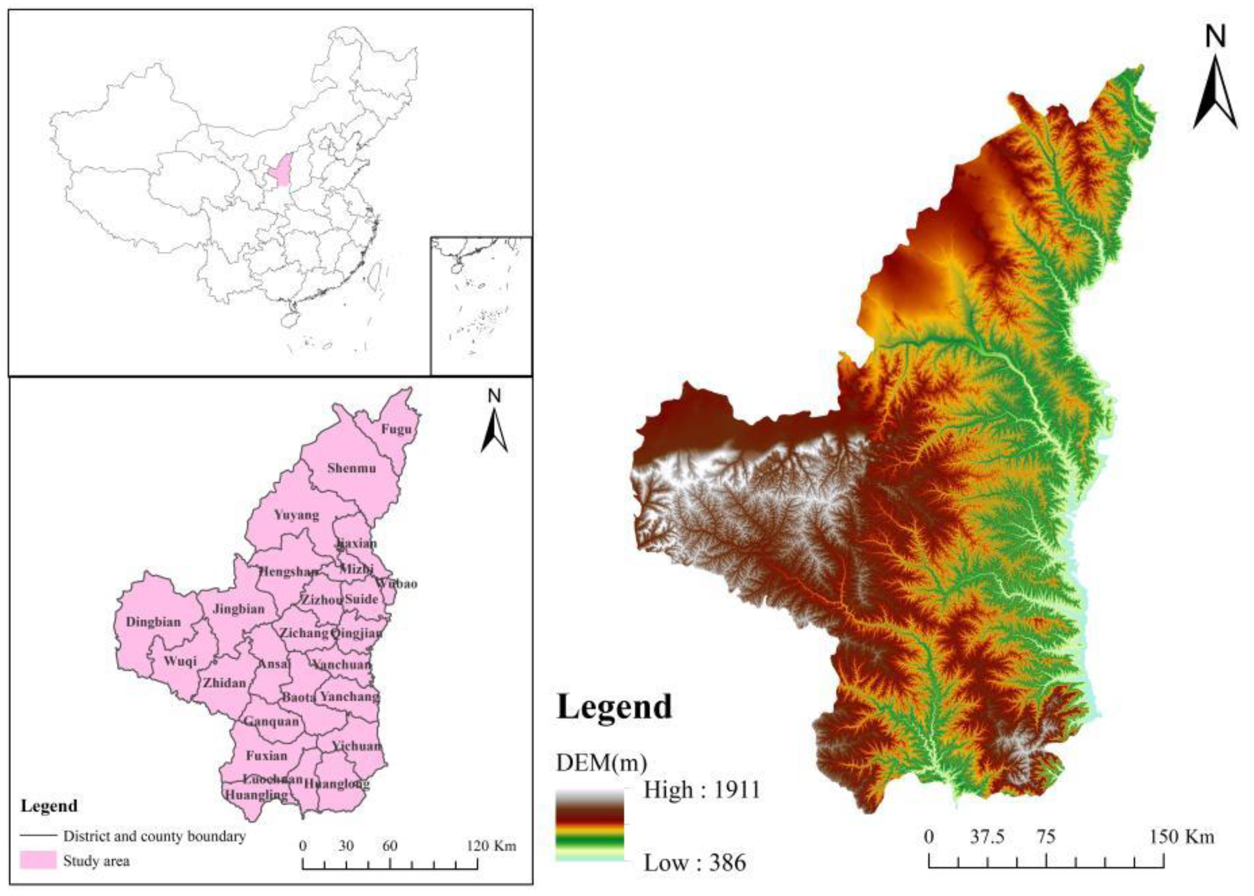
The study region’s natural surroundings in the Loess Plateau, with low annual precipitation, low vegetation cover, steep terrain, loose soils, and the constant disturbance of human activities, have caused a highly vulnerable biological environment to develop, with land desertification, soil erosion, and salinization. Zhang et al. analyzed the extent to which land-use change has an impact on the ESV as well as the coordination between ecological and environmental quality and socioeconomic development [29]. Jiang et al. used a mix of benefit transfer and proxies for land-use and land cover to study the ESV resulting from changes in the land-use and land cover on the Loess Plateau between 1990 and 2015 [30]. Fang et al. examined and evaluated the connection between the ESV and land-use patterns, as well as assessing the association between land-use change and the ESV at the town scale [31]. Therefore, in the Loess Plateau, studies on ecosystem services have mainly focused on analyzing the effects of land-use/cover changes on the ESV within the Loess Plateau region, while fewer studies have been conducted to examine the mechanisms, quantify the effects of various environmental and societal factors on the ESV, and forecast future trends in the field. In this study, based on the investigation of the ESV distribution and change in the Loess Plateau of Northern Shaanxi from 2000 to 2020, the influence status of multiple factors on the ESV was focused on and the future development trend was predicted. The objective of this study is to address the following questions: (1) What are the ESV’s temporal trends and regional distributions in the Loess Plateau of Northern Shaanxi from 2000 to 2020? (2) What is the degree of influence of various factors on the ESV in the Loess Plateau of Northern Shaanxi? (3) What is the status of the integrated constraints on ecosystem development within the Loess Plateau of Northern Shaanxi? (4) What is the future development trend of the ecological environment of the Loess Plateau in Northern Shaanxi?

2. Materials and Methods

2.1. Study Area

The study area is in the heart of the Loess Plateau. It consists of two prefecture-level cities, Yan’an and Yulin (Figure 1). The area is a paleotopography formed by Mesozoic bedrock, covered with a thick layer of loess and red soil from the Cenozoic, and then formed by cutting with running water. It is in the transition zone from semiarid to arid, the annual average temperature is approximately 8–14 °C, and the annual rainfall is approximately 350–660 mm. The spatial distribution reveals that the northwest receives less precipitation than the southeast due to an irregular seasonal distribution. The precipitation is mainly concentrated in summer and the precipitation intensity is high. It often appears in the form of heavy rain.

2.2. Data

The average temperature and annual precipitation data in 2000, 2010, and 2020 used were derived from the “Shaanxi Provincial Statistical Yearbook” and “China Environmental Bulletin” of each year. The land-use data for 2000, 2010, and 2020 were from the GlobeLand30 platform (http://globeland30.org/, accessed on 18 January 2022) and were divided into seven types: cropland, forestland, grassland, wetland, water bodies, construction land, and unused land. The slope and elevation data were from the Chinese Academy of Sciences Geospatial Data Cloud Platform (http://www.gscloud.cn/, accessed on 10 February 2022). The annual-rainfall, annual average temperature, population density, and soil-type data were from the Resource and Environmental Science and Data Center of Chinese Academy of Sciences (http://www.resdc.cn/, accessed on 10 February 2022). The main road data came from the BIGEMAP platform (http://www.bigemap.com/, accessed on 10 February 2022).

2.3. Methods

2.3.1. Miami Model

Xie et al. [32] proposed the ESV-equivalent factor per unit area of the Chinese ecosystem, which has been widely applied by many scholars in many aspects [33,34,35]. However, since it is based on the national average level, the ESV needs be adjusted to account for regional variations in a small area when it is calculated. The climatic productivity of an area is a key factor affecting its ecological environment and the ESV [36]. Therefore, this study calculated the climatic productivity of the area as well as the national average climatic productivity to obtain the regional difference coefficient and then revised the equivalent factor [37]. The ESV was calculated using the revised equivalent factor in combination with the land-use status of the study area.
Using the Miami model to calculate climate productivity, the specific formula is as follows:
np p R = 30000 × ( 1 e 0.000664 R )  
  npp T = 30000 1 + e 1.315 0.119 T
  npp p = MIN { npp T , npp R }  
where R is the annual precipitation, T is the annual average temperature, n p p R is the net primary productivity of vegetation calculated using the annual precipitation, and n p p T is the net primary productivity of vegetation calculated using the annual average temperature. According to Liebig’s law of least factor, n p p p takes the minimum of n p p R and n p p T as the regional climate productivity.
  S k = npp k npp
where n p p is the national average climate productivity, n p p k is the climate productivity of the study area, and S k is the regional difference coefficient.
The following is the formula for calculating the economic value of an equivalent factor in the study area:
  E a = E a × S k
where E a is the value corresponding to an equivalent factor nationwide (CNY 449.1/hm2).

2.3.2. Spatial-Autocorrelation-Analysis Method

The possible dependency of the observation data of variables in the same distribution region is referred to as spatial autocorrelation [38], which is one of the effective methods used to analyze the spatial correlation of the same variable between different observation objects [39,40]. In this study, spatial autocorrelation analysis was used to explore the spatial distribution pattern of the ESV. The global spatial autocorrelation and local spatial autocorrelation were used to investigate the overall distribution characteristics of the ESV in the study area and the correlation degree of the ESV between each district and neighboring districts and counties, respectively.
Global spatial autocorrelation:
Global spatial autocorrelation can reflect the general trend of spatial correlation within the entire study area [41]. The specific formula is as follows:
I = i = 1 n j = 1 n W i j · ( Y i   Y ¯ ) · ( Y j   Y ¯ ) S 2 · i = 1 n j = 1 n W ij
where I is the global spatial autocorrelation index,   S 2 = 1 n i = 1 n ( Y i Y ¯ ) ,   Y i is the ESV of the county (district), n is the number of counties (districts), and W i j   is the spatial weight matrix.
Local spatial autocorrelation:
While global spatial autocorrelation cannot highlight the aggregation state of local area units, local spatial autocorrelation can accurately capture the aggregation and divergence characteristics of spatial units and neighboring units [42].
I i = ( Y i   Y ¯ ) S 2 j n W ij · ( X i   X ¯ )
where I i represents the local spatial autocorrelation Moran index, and the other variables have the same meaning as in Equation (6).

2.3.3. Entropy Weight Method

The entropy weight method is an objective assignment method [43]. According to the explanation of the basic principles of information theory, entropy and information are measurements of the degree of disorder and order of a system, respectively [44]. If the index’s information entropy is lower, its weight should be higher and its role in the comprehensive evaluation should be larger because it provides more information [45]. The entropy weight method overcomes the influence of human subjective consciousness and makes the evaluation results more objective [46]. In this study, based on the quantitative analysis of the influence of each factor on the ESV, the entropy weight method was used to calculate the weights of each influencing factor, analyze the specific reasons limiting the development of the ESV, and used in the subsequent comprehensive impact zoning study. Its specific calculation process is divided into the following three steps:
Data standardization:
{ P ij = x ij x ijmin x ijmax x ijmin           Positive   indicator P ij = x ijmax x ij x ijmax x ijmin           Negative   indicator
Information entropy calculation:
E j = l n ( n ) 1 i = 1 n p i j l n p i j
where p i j = Y i j / i = 1 n Y i j ; if p i j = 0, then define lim p i j 0 p i j l n p i j = 0 .
Calculation of the weight of each indicator through information entropy:
W i = 1 E i k   E i   ( i = 1 , 2 , , k )

2.3.4. CA–Markov Model

The CA–Markov model combines the spatial dynamic evolution capability of cellular automata and the time dynamic advantage of the Markov model [47,48,49,50]. This model has good predictive ability in landscape pattern research evolution and land-use dynamic change [51].
Cellular automata are defined as cells with states that are discrete and finite in a cellular space. This represents a dynamic system that follows certain regional laws as it develops in a discrete time dimension. The most basic components of cellular automata include the cellular unit, cellular space, domain, and rules [52,53]. It can usually be expressed as follows:
S t + 1 = f ( S t , N )
where S is a set of discrete and finite states of the cellular, t and t + 1 represent time, f is the transformation rule of the local cellular space, and N is the neighborhood of the cellular unit. At present, cellular automata are widely applied in population distribution change, land-use change, forest fires, and other aspects [54].
The Markov model is a method of stochastic process theory formation proposed by Russian mathematician Markov. It calculates the probability of things in the initial period of different states and the transition probability between states and then shows the trend of transformation between different states to realize the prediction of the future state of things [55,56]. In the process of Markov model prediction, the state of things in a past moment has nothing to do with the development of the state. So, the transfer process has no aftereffect [57], which is called the Markov process.
P = P ij = [ P 11 P 1 n P n 1 P nn ]
where P i j is the transition probability matrix of the land-use change state, 0 P i j < 1 , and j = 1 n P ij = 1 , i ,   j = 1 ,   2   is the land type; in this paper, n = 7 .
In this study, the trend forecast of the ESV for 2030 in the study area was achieved by means of the CA–Markov model. The data of 2000 and 2010 were used to forecast the study area in 2020 before conducting the analysis, and the accuracy was compared with the actual condition in 2020, and the accuracy was verified to be qualified before conducting the subsequent forecast. Additionally, the forecast was made by adding constraints, such as elevation, slope, water body, distance from a road, and distance from a water body, to create an adaptation atlas to ensure the forecast results are more realistic.

3. Results

3.1. Land-Use Status Analysis

Through analysis, the land-use map of the study area from 2000 to 2020 was obtained (Figure 2). It was found that the area of grassland was the largest in the area, with an area of more than 45% in the three phases, followed by cropland, accounting for more than 32%. Wetland accounted for the smallest area, with a ratio of 0.18% (2000)–0.05% (2020). The sum of grassland, cropland, and forestland accounted for 96.19% (2020)–97.24% (2000) of the total size of the study area. The amount of construction land exhibited an upward trend, from 0.36% in 2000 to 1.68% in 2020, and the growth rate accelerated year-by-year. The area of wetlands in the study area decreased by 64.38% from 2000 to 2010, followed by water bodies, which decreased by 36.90%, and construction land grew the most, with an increase of 55.90%. From 2010 to 2020, the wetland in the study area decreased by 30.77% and the construction land increased by 199.55% (Figure 3).

3.2. ESV Analysis

3.2.1. Revision of the ESV

According to the annual average temperature and annual precipitation data of the area and the whole country (Table 1), the climatic productivity of the study area was calculated to be 770.81, the national average climatic productivity was 838.27, the regional coefficient was 0.92, and the equivalent factor’s corresponding value in the area was CNY 412.96/hm2 (Table 2).

3.2.2. Changes in the ESV

Table 3 shows that the ESV of the study area in 2000, 2010, and 2020 was CNY 44.390 billion, 43.824 billion, and 43.475 billion, respectively, with an overall decrease of CNY 915 million, or 2.06%. From 2000 to 2010, the total value decreased by CNY 566 million, or 1.28%. From 2010 to 2020, the total value decreased by CNY 349 million, or 0.80%, indicating a slower decrease rate.
In terms of individual types, the total ESV of grassland and forestland was relatively high, while the value of unused land and wetland was low. Although wetland had the highest value per unit area, their area was smaller, so they provided lower values. The unused land refers to the natural covered land with vegetation coverage less than 10%, which had a low ecological service function.

3.2.3. Changes in the Individual ESV

Table 4 shows that the single ESVs of food production, gas regulation, climate regulation, hydrological regulation, waste disposal, soil conservation, maintenance of biodiversity, and landscape provision in the study area from 2000 to 2020 all decreased. Among them, the hydrological regulation value decreased the most, by CNY 205 million, and the food production value decreased the least, by CNY 9.25 million. The value of soil conservation over the years was the highest and food production value was the lowest.

3.2.4. Changes in the ESV at the District and County Scales

The land-use status within the 25 districts and counties in the study area was obtained separately by district and county, and then the ESV per unit area within each district and county was calculated for 2000, 2010, and 2020. According to Figure 4, the ESV distribution in the study area was typically higher in the south and lower in the north. From 2000 to 2020, the ESV per unit area in Huanglong County was the highest among the 25 counties, with CNY 10,589/hm2, CNY 10,604/hm2, and CNY 10,429/hm2, while the ESV per unit area in Suide County was only CNY 3656/hm2, CNY 3637/hm2, and CNY 3607/hm2.
By analyzing the changes in the ESV per unit area of each district and county (Figure 5), it was found that, from 2000 to 2010, the ESV per unit area decreased in 19 districts and counties and increased in 6 districts. From 2010 to 2020, the number of counties with a decreasing ESV per unit area was 16 and the number of counties with increasing values was 9. Overall, the unit area value of most of the districts and counties showed a decreasing trend from 2000 to 2020, and the ecological condition of the area was deteriorating.

3.3. The Spatial Distribution Pattern of the ESV

3.3.1. Global Spatial Autocorrelation Analysis

Scatter plots of Moran’s I index for 2000, 2010, and 2020 were obtained by means of global spatial autocorrelation analysis (Figure 6). Figure 6 shows that the global Moran’s I indexes for the ESV per unit area in 2000, 2010, and 2020 for 25 districts and counties in the area were 0.666, 0.661, and 0.670, respectively, which were all greater than 0. The results show that the unit ESV of the 25 districts and counties showed a strong positive correlation in each year and the spatial distribution showed obvious clustering characteristics.

3.3.2. Local Spatial Autocorrelation Analysis

To determine whether there was a local agglomeration effect among the 25 districts and counties in the area, the local Moran’s I (LISA) value was calculated through local spatial correlation analysis and a LISA distribution map was created (Figure 7).
Figure 7 shows that local spatial autocorrelation pattern of the ESV per unit area of the 25 districts and counties showed a “high-high” agglomeration area and a “low-low” agglomeration area. There was no “high-low” agglomeration area or “low-high” agglomeration area. The “high-high” agglomeration area was distributed in the south of the study area, namely, Fuxian County, Luochuan County, Yichuan County, and so on. The unit ESV of these areas had a strong positive spatial correlation mechanism and improved the unit-area ESV of the surrounding area. The “low-low” agglomeration areas were primarily distributed in the central and northern areas of the study area, namely, Hengshan County, Jia County, Suide County, Zizhou County, etc., indicating that the ESV per unit area of these areas and the ESV per unit area of the neighboring areas had a positive correlation with each other at a low level.

3.4. Influencing Factors of the ESV

The spatial distribution maps of different influencing factors were obtained, and different levels were assigned according to the magnitude of the values, which are overlaid with the land-use maps to calculate the ESV of the corresponding level according to the land-use status within the different levels of each factor, so as to investigate the influence of each factor on the ESV status.

3.4.1. Impact of Annual Rainfall on the ESV

The annual rainfall data were reclassified into four levels: below 400 mm, 400–500 mm, 500–600 mm, and above 600 mm. Table 5 shows that, with the increase in rainfall, the ESV per year with an annual rainfall of more than 600 mm was 2.57 times that of the area with an annual rainfall of less than 400 mm, indicating that rainfall had a great impact on the ESV in this area. According to comparison of land-use status, forestland accounted for 85.23% in areas with an annual rainfall above 600 mm and only 0.13% in areas with rainfall below 400 mm, indicating that vegetation grew vigorously in areas with abundant precipitation and had a high ESV.

3.4.2. Impact of Temperature on the ESV

The annual average temperature data were reclassified into four levels: below 8 °C, 8–9 °C, 9–10 °C, and above 10 °C. Table 6 shows that, with the increase in the annual average temperature, the ESV per unit area showed an increasing trend, with a total increase of 41.00%. According to the analysis of land-use status, cropland, forestland, and grassland accounted for 98.58% of the area above 10 °C and unused land accounted for the lowest proportion, among which 47.28% of forestland and 43.12% of water bodies were distributed in this area. This result indicated that the area with higher hydrothermal conditions had a strong ecological function and a high ESV.

3.4.3. Impact of Slope on the ESV

The slope data were reclassified into five levels: 0–2°, 2–6°, 6–15°, 15–25°, and above 25°. Table 7 shows that the ESV per unit area in the 0–25° region showed an increasing trend, increasing by 57.03%. When the slope was greater than 25°, the ESV decreased, but only by 4.58%. In the 0–2° area, forestland accounted for only 2.53% and contained 47.47% of the construction land and 76.81% of the unused land. In the area above 15°, grassland and forestland accounted for 72.28%, playing a strong ecological function. Therefore, slope was positively correlated with the ESV.

3.4.4. Impact of Soil Types on the ESV

According to the traditional classification system of soil occurrence, the soil types were divided into 10 types, including semileached soil, calcium-layer soil, arid soil, primordial soil, etc. Table 8 shows that different soil types had different impacts on the ESV, with great differences. The unit area value of lakes and reservoirs was the highest, while the unit area value of artificial soil was the lowest. In lakes and reservoirs, the proportion of unused land and construction land was 0, as water bodies occupied the majority of the region and had a strong ecological function, and so this soil type had a high ESV per unit area. In the artificial soil, cropland accounted for 74.34%, which was due to long-term production activities. After fertilization, irrigation, farming, and other agricultural measures, the amount of cropland rose, as did its value, in line with the characteristics of artificial soil.

3.4.5. Impact of Elevation on the ESV

The elevation data were reclassified into four levels: below 1000 m, 1000–1200 m, 1200–1400 m, and above 1400 m. As shown in Table 9, the ESV in higher-elevation locations was frequently higher than that in regions with lower elevations. The ESV was the lowest in areas below 1000 m, and the ESV per unit area of 1200–1400 m was the highest, which was 1.25 times that of the area below 1000 m. Construction land was extensively dispersed in the low-altitude region, as per a comparison of land-use. A total of 65.10% of the construction land was distributed below 1200 m and human activity had a significant influence. Only 8.97% of the forestland was distributed lower than 1000 m, while 67.73% of the forestland was distributed in the area above 1200 m. This shows that the high-altitude area had less human intervention, a good ecological environment, and a strong ecological function.

3.4.6. Impact of Population Density on the ESV

The population density data were reclassified into four levels: less than 40 people/km2, 40–80 people/km2, 80–120 people/km2, and more than 120 people/km2. Table 10 shows that, with the increase in population density, the ESV per unit area showed a decreasing trend. The ESV per unit area in areas with a population density below 40 people/km2 was 1.62 times that in areas with a population density above 120 people/km2. In the area with less than 40 people/km2, forestland and grassland accounted for 46.34% and 32.12%, respectively, and construction land accounted for 0.19%. Wetland was also mainly distributed here, while in areas with more than 120 people/km2, cropland accounted for 50.52%, construction land accounted for 2.77%, and 44.54% of construction land was distributed here, indicating that, in areas with less population, human activity intensity was weak, vegetation coverage was high, the ecosystem was stable, and service value was great, but, in densely populated regions, people’s intense social and economic activity would undoubtedly have some negative effects on the ecological environment, which would subsequently restrict the ESV.

3.4.7. Impact of Roads on the ESV

The main roads were established to obtain regions within 2 km, 2–4 km, 4–6 km, and more than 6 km away from a road. Table 11 shows that, with the increase in the distance from the main roads, the ESV per unit area continued to increase. From areas within 2 km to areas beyond 6 km, the ESV per unit area increased by 16.93%. Among them, forestland accounted for only 12.37% in areas within 2 km from a road and 20.78% in areas more than 6 km away from a road, construction land accounted for 6.09% in areas within 2 km and 0.71% in areas more than 6 km away from a road, and the unit area wetland value in areas more than 6 km away from a road was much higher than other regions.

3.5. Weight Analysis of Influencing Factors and Comprehensive Evaluation

3.5.1. Weighting Analysis of Influencing Factors

To comprehensively reflect how the aforementioned seven natural and societal factors affect the ESV in the area, the unit area value of each grade of each factor was calculated based on the above quantification. The entropy weight method index calculation formula was used to standardize the unit area value of the different grades of each factor through the standardization formula to calculate its information entropy. Finally, information entropy was used to calculate each factor’s weight.
Figure 8 shows that the seven natural and social factors influenced the ESV in descending order of weight: population density (0.309), rainfall (0.165), soil type (0.116), slope (0.109), elevation (0.106), annual average temperature (0.100), and distance from the road (0.096). The highest weight was given to population density and the lowest weight was given to distance from a road. Therefore, human activities disturbed the ecosystem the most among the many influencing factors. In addition, due to the limited space occupied by roads, they provided less interference with the ecological environment in areas far away from roads.

3.5.2. Comprehensive Evaluation of Influencing Factors

To determine the comprehensive influence size of the seven factors on the ESV of the study area, the weights of the factors were multiplied by the corresponding ESV per unit area of each level based on the weights of the factors previously calculated. According to Jenks, four categories were used to divide the area: mild-impact zone, moderate-impact zone, severe-impact zone, and extreme-impact zone. The zoning map of the impact of the ESV in the area was generated.
Figure 9 shows that the influence of natural and social factors on the ESV showed obvious geographical distribution characteristics, which were mainly reflected in the higher degree of influence in the northern area and the lower degree of influence in the southern area. From north to south, there was a weakening tendency that was constant. Comparing the ESV distribution and land-use status, it was found that mild- and moderate-impact zones were basically distributed in zones with vigorous vegetation growth and a high ESV, indicating that the low-impact zones had high ecological environment quality. In more severe impact zones, strong disturbances from artificial and natural conditions affected the performance of ecological functions. A degree of ecological function would be impacted by excessive human interference.

3.6. Forecast of the ESV Trend

Before making a forecast, the land-use status maps in 2000 and 2010 were used to generate the forecast map of the study area in 2020 and for comparison with the real land-use map from 2020. After accuracy verification, the Kappa coefficient was 0.75, which showed that the forecast result based on the CA–Markov model in the area was relatively accurate and this method could be used to predict its future changes. In turn, the land-use status of the region in 2030 was forecasted (Figure 10).
Table 12 shows that the total ESV in 2030 was CNY 43.436 million, CNY 39 million lower than that in 2020. The value provided by grassland decreased the most, while the value of forestland increased the most. Among them, grassland, wetland, and unused land values fell by CNY 315, 16, and 4 million, respectively. The values of forestland, cropland, and water bodies increased by CNY 222, 62, and 4 million, respectively. Comparing the predicted land-use status, it was found that the construction land area in 2030 had increased by 22.30% compared to 2020. The ecological resources were quickly consumed because of the rapid growth of construction land, which reduced the ESV and weakened ecological functions. Therefore, in the future, it is necessary to further strengthen the protection and construction of the ecological environment of the area to prevent the appearance of negative results.

4. Discussion

4.1. Temporal and Spatial Change Mechanism of the ESV

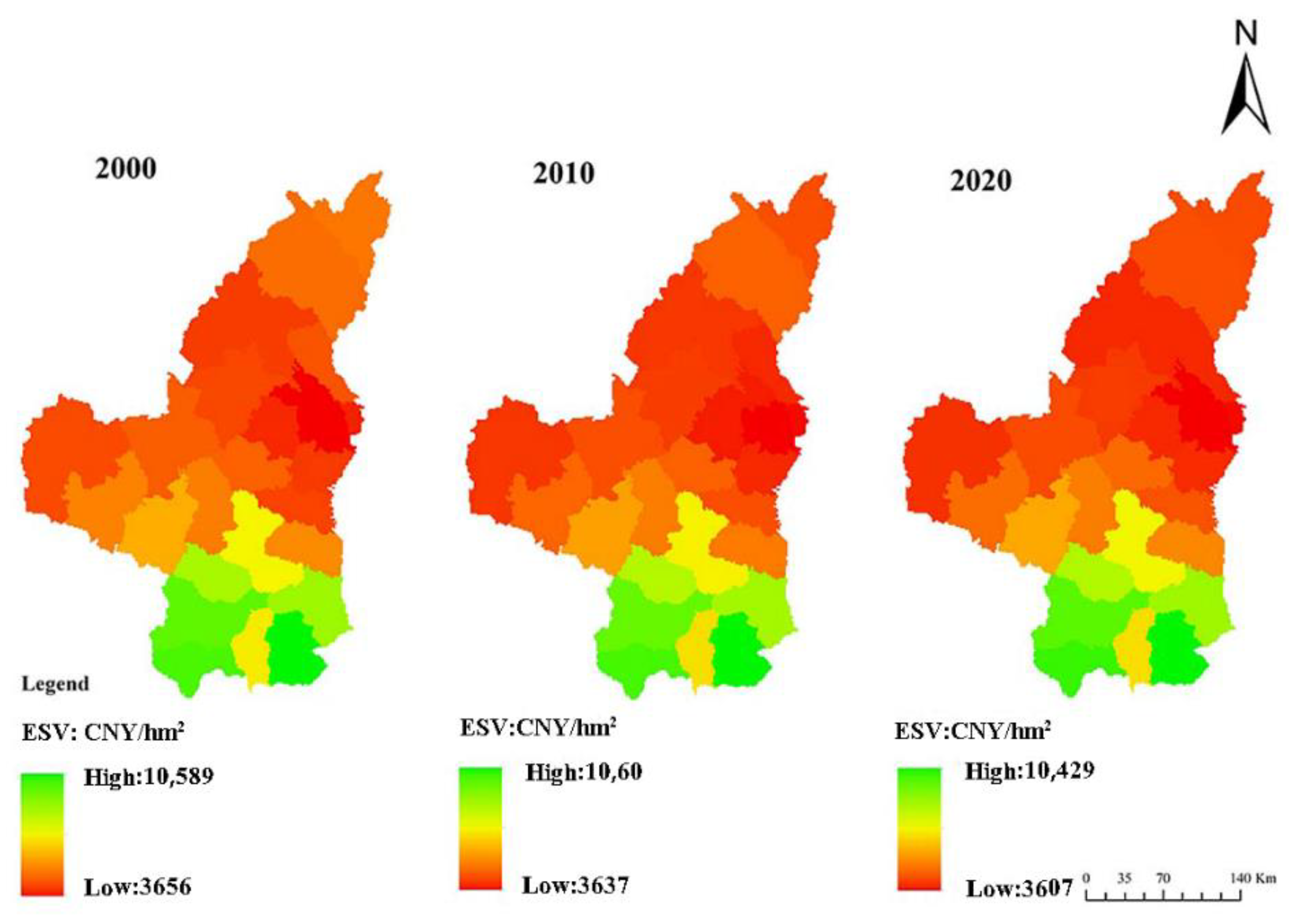
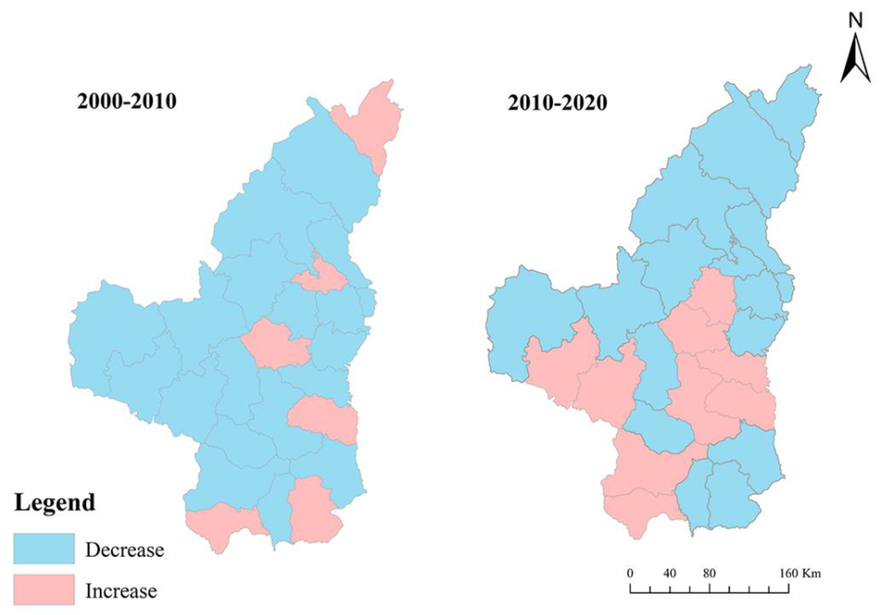
In this study, we found that there were significant temporal dynamics and spatial heterogeneity of the ESV in the Loess Plateau region of Northern Shaanxi. This region has seen a large change in land-use status in the last 20 years, and this has led to changes in the ecosystem services of the region and their values. Construction land is a nonecosystem service site and therefore has a null ESV [58,59,60]. Additionally, within the region from 2000 to 2020, the ESV has been decreasing with increasing construction land and cropland. Numerous studies have found that urban expansion and the increase in cropland come at the cost of high-ESV lands such as forestland and grassland [61,62]. These lands occupy and affect other ecological lands, leading to the decrease in the ESV. This is consistent with the results of our study. Additionally, in our study, the ESV in the study area showed a trend of being high in the south and low in the north. After the analysis, it was found that Northern Shaanxi is a relatively rich region of coal resources in China, and coal resources are more concentrated in the northern part of the study area, near Shenmu City, Fugu County, Yulin City, etc. The concentrated coal mining has caused damage to the surrounding ecological environment to some extent. Qian et al. found that mining activities in the southern Qilian Mountains caused significant ESV losses to the grassland and wetland [63]. Gao et al. found that the dramatic expansion of mining land had destroyed large areas of forestland and reduced the ESV [64]. The southern part of the study area, Huanglong County, is one of the eight major forest areas in China. It is also a protective forest area of the Loess Plateau. The proportion of forestland in the area was above 85% in all years, and the vegetation grows vigorously. The study of this region is important for the conservation of regional biodiversity and the maintenance of ecological balance [
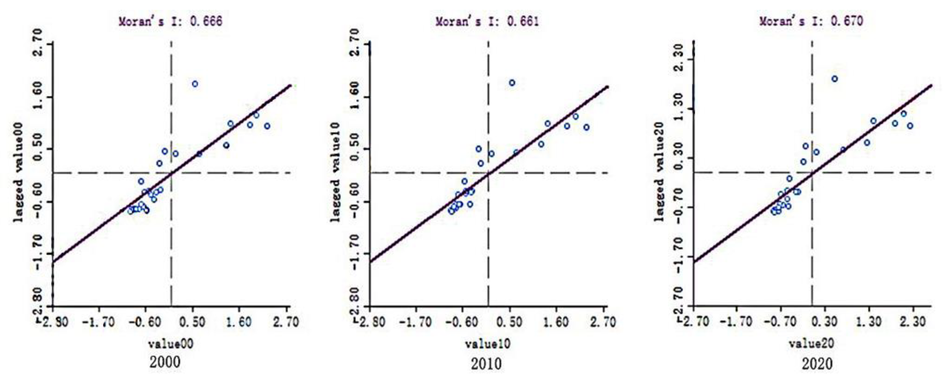
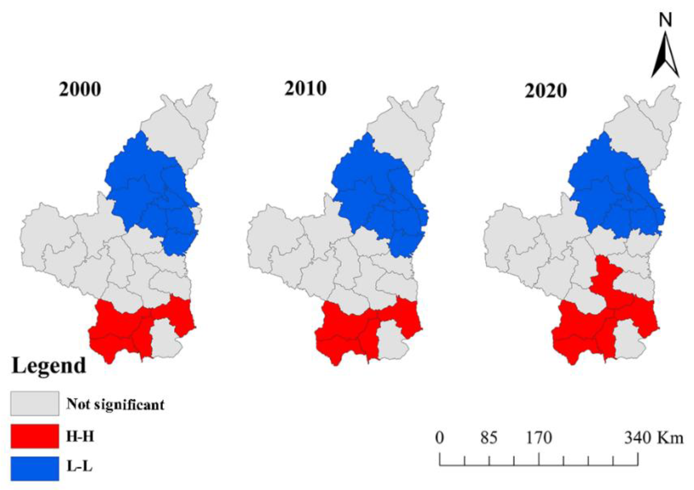
65]. Therefore, the ESV was higher in the southern part of the study area. In addition, the spatial autocorrelation model was used to analyze the spatial aggregation pattern and association pattern of the ESV, which can further reveal the spatial differentiation characteristics of the ESV in the study area [66]. In this study, a high-high aggregation area in the south and a low-low aggregation area in the northcentral part were identified, respectively. This indicates that the ESV in the study area has obvious spatial aggregation characteristics.

4.2. Influencing of Various Factors on the ESV

The constant changes in the ESV are influenced by multiple natural and social factors [67,68,69]. In this study, the effect of each factor on the regional ESV was found to be negatively correlated with population density and the ESV. The effect of soil type on the ESV was determined by the nature of the soil itself. The other five factors were positively correlated with the ESV. These findings are consistent with previous studies [70,71]. Analysis of the weight of each factor on the ESV using the entropy weighting method revealed that population density, rainfall, and soil type in the study area have a greater effect on the ESV, and the distance from a road has the least effect. Human activities disturb local ecosystems, altering the ecological environment and affecting ecological functions, leading to a decrease in the ESV. Guo et al. found that population density was the most important factor influencing the ESV in the region of Funiu Mountain [72]. In addition, areas with high rainfall have good hydrothermal conditions that are more suitable for vegetation growth and have more complex ecosystems. Meanwhile, low rainfall causes the ecological function of the area to be weakened. Xie et al. found that the ESV in China gradually decreased from the rainfed southeast to the arid northwest [73]. Zhao et al. found that precipitation has an important impact on ecosystem services in the Yangtze River Delta region [74]. In this study, although roads are also the result of human production and construction, they only have a small impact on the ESV in a limited area of their proximity due to the limitation of their own functional performance. Therefore, the degree of impact is relatively small. After a comprehensive evaluation by using the weights of each factor, it was found that the ESV was high in the areas with a low impact and low in the areas with a high impact in the study area. This indicates that the ESV is higher in areas with abundant precipitation, sufficient sunshine, high elevation, a gentle slope, and low human intervention. However, excessive human intervention can affect ecosystem function [75]. Therefore, if the various factors mentioned above are adjusted in the future, a good ecological environment in the study area can be maintained.

4.3. Trend Forecast Analysis of the ESV

Forecasting of the regional ecological environment enables us to anticipate the future development trend of the ecological environment. Forecasting furthers our understanding of the regional ecological security situation in order to facilitate constructive suggestions for ecological environment improvement and protection [76]. CA models have powerful computational capabilities to solve complex system problems and have been widely used in land-use [77,78]. However, it is difficult for a single model to achieve a reasonable prediction of land-use change. Some scholars have coupled the CA model with logistic functions, artificial neural network models, and SD models to carry out research on the dynamic prediction of land-use [79,80,81]. However, the above integrated models are difficult to achieve in terms of nonlinear representation, parameter optimization, operability, and so on [82,83,84]. However, the CA–Markov model is more scientific and applicable. It can make the prediction results more accurate [85]. In this study, the CA–Markov model was used to impose the corresponding constraints to achieve the prediction of land-use in the study area and calculate the ESV. The results show that the ESV of the study area will decrease by 2030. This is mainly due to the continuous increase in construction land. Therefore, further rational planning of each land-use type is needed to promote the improvement of ecological service quality.

4.4. Policy Implications

First, after the analysis, we found that human activities have the strongest influence on the ecological environment within the Loess Plateau area in Northern Shaanxi. Therefore, in order to further control the interference of human activities, we need to establish reasonable ecological protection zones within the study area. Human activities are restricted within the protected areas to protect the ecological environment and biodiversity. Meanwhile, in regional territorial spatial planning, three control lines of the ecological protection red line, permanent basic agricultural land, and urban development boundary should be determined. The government should develop the regional economy and ecological security at the same time so as to coordinate regional development and ecological stability and prevent economic development at the expense of ecological environment [86].
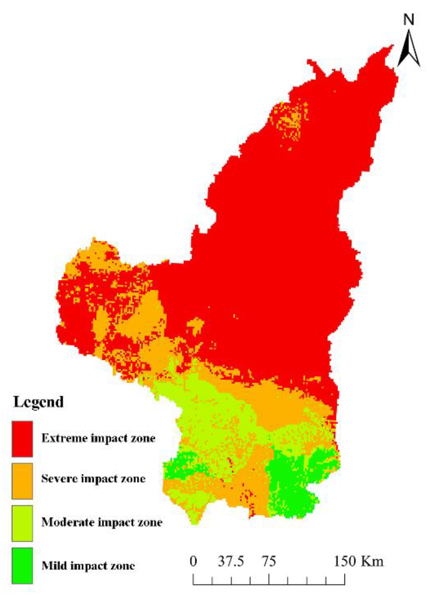
Second, according to the results of the comprehensive zoning evaluation of each impact factor, the zoning is based on the degree of impact. Different environmental improvement measures were implemented in the study area for different impact zones. The extremely heavy-impact area and heavy-impact area are mainly located in the northcentral part of the study area. This area is characterized by a steep terrain, strong human interference, and relatively fragile ecological environment. Therefore, the utilization rate of construction land and vegetation coverage should be further improved in this area, and ecological protection projects should be vigorously carried out. Thus, the stability and health of the ecosystem should be maintained. For the moderately and lightly affected areas distributed in the south, we should continue to do a good job of protecting the ecological environment of the area, controlling large areas of unreasonable grazing, and protecting water resources.
Third, Northern Shaanxi is extremely rich in mineral resources. However, extensive mining activities have caused groundwater pollution, surface landscape fragmentation, ground subsidence, soil quality decline, and other environmental problems [87]. Measures should be taken to protect and restore the ecological environment of mining areas. Hu et al. proposed measures alongside mining to restore the ecological environment of the mining area [88]. Bi et al. proposed the use of microorganisms to improve the quality of the soil in the mining area [89]. Therefore, the corresponding methods for the ecological management of mining areas need to be proposed according to the mining characteristics of the study area so that the ecological condition of the entire Northern Shaanxi Loess Plateau can be improved.

4.5. Limitations and Future Work

The findings of this study offer some reference value for the future sustainable development and ecological environment of the region; however, there are some limitations to this study. The differences between different regions were affected by natural, social, and economic factors. In this study, the ESV’s equivalent factor was revised by calculating regional and national climate productivity, which is not comprehensive enough. In addition, in analyzing the factors affecting the ESV, this study selected annual rainfall, population density, roads, and other factors for analysis. Although both natural and social factors were included, the consideration of the factors still had some limitations. Therefore, there will be some differences between the established impact zone and the actual situation. Finally, when using the CA–Markov model for trend forecasting, the elevation, slope, water bodies, distance from the road, and distance from a water body were added, and the policy factors for future development in the area were not fully taken into account. Combined with the model itself being restricted, there will be some differences between the predicted results and the actual development in the future.

5. Conclusions

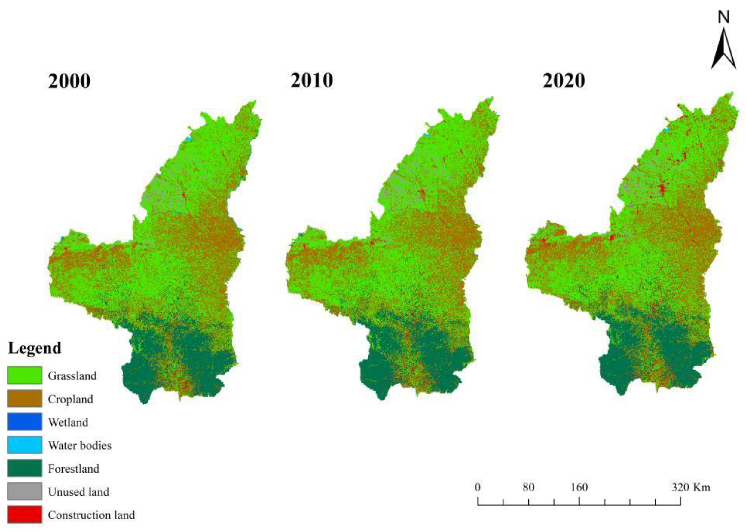
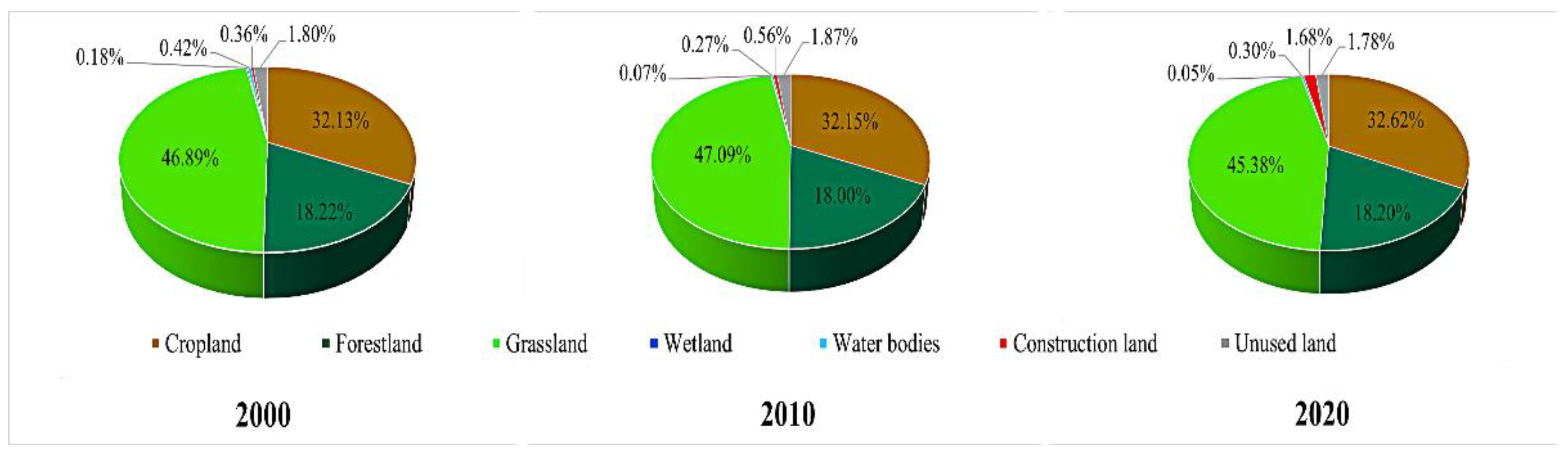
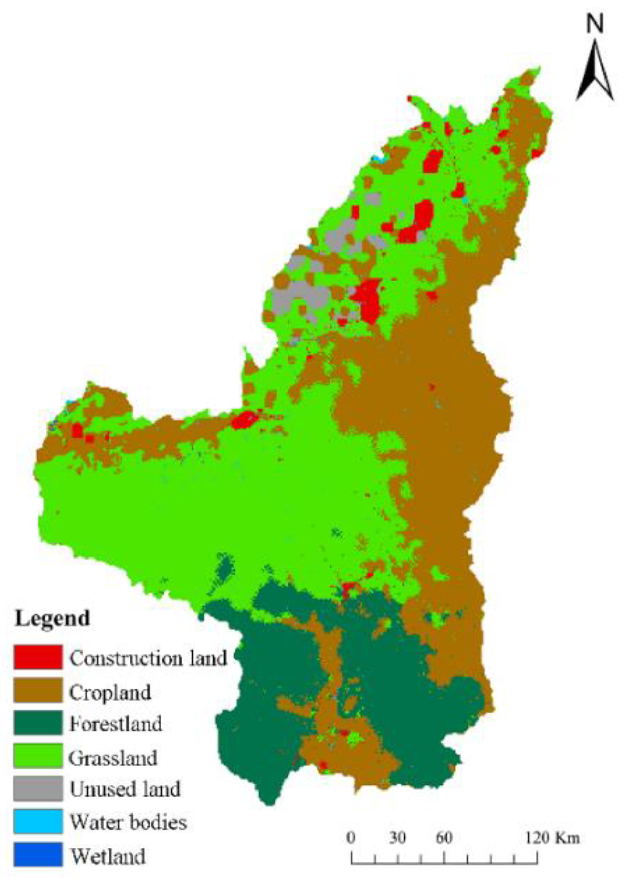
In this study, the temporal and spatial changes in the Loess Plateau of Northern Shaanxi based on the calculation of the ESV were analyzed, and an impact zoning map was established by quantifying various influencing factors. Finally, the future development trend of the ESV was predicted. The following conclusions can be reached: (1) The land-use types were mainly grassland, forestland, and cropland, and the combined area of the three types covered more than 95% of the area. In addition, construction land in the study area increased the fastest, with a 4.6-fold increase from 2000 to 2020. (2) From 2000 to 2020, the ESV decreased continuously, and a pattern of being high in the south and low in the north was evident in the spatial features. (3) The weighting analysis of influencing factors showed that population density (0.309) > rainfall (0.165) > soil type (0.116) > slope (0.109) > elevation (0.106) > annual average temperature (0.100) > and distance from a road (0.096). By establishing the impact zones, it was found that the degree of impact decreases from south to north in the area. (4) It is predicted that the ESV will remain reduced by 2030 compared to 2020 in the area.
The ESV is affected by a combination of factors. Natural factors create the foundation of the ecosystem, and with rapid socioeconomic development, humans will continue to impose on this foundation, making the ecosystem more and more unstable. Positive human behaviors lead to stronger ecosystem functions, while negative human behaviors disrupt the ecological balance and cause the ecosystem to evolve in an unsustainable direction. In this study, the factors that influence the ESV were considered and different impact areas were classified to understand the regional ecological quality, identify the root causes that limit the function of ecosystems, and predict the future development trend. The research results provide a scientific basis for ecological environmental protection and policy formulation in the Loess Plateau of Northern Shaanxi.

Author Contributions

Y.Z. and X.J. provided the idea, supervision, and drafted and revised the manuscript. L.Z. and Q.M. carried out the experiments and drafted and revised the manuscript. L.H., Z.L., P.Z. and M.Z. provided useful suggestions. All authors have read and agreed to the published version of the manuscript.

Funding

This research was funded by the Fund Project of Key Laboratory of Degraded and Unused Land Consolidation Engineering, the Ministry of Natural and Resources (program no. SXDJ2019-03) and the Fundamental Research Funds for the Central Universities, CHD (300102270206 and 300102278403).

Institutional Review Board Statement

Not applicable.

Informed Consent Statement

Not applicable.

Data Availability Statement

Not applicable.

Acknowledgments

We acknowledge all who contributed to the data collection and processing, as well as the constructive and insightful comments by the editor and anonymous reviewers.

Conflicts of Interest

The authors declare no conflict of interest.

References

  1. Costanza, R.; d’Arge, R.; de Groot, R.; Farber, S.; Grasso, M.; Hannon, B.; Limburg, K.; Naeem, S.; O’Neill, R.V.; Paruelo, J.; et al. The value of the world’s ecosystem services and natural capital. Nature 1997, 387, 253–260. [Google Scholar] [CrossRef]
  2. Finlayson, M.; Cruz, R.; Davidson, N.; Alder, J.; Cork, S.; de Groot, R.; Lévêque, C.; Milton, G.; Peterson, G.; Pritchard, D. Millennium Ecosystem Assessment: Ecosystems and Human Well-Being: Wetlands and Water Synthesis; Island Press: Washington, DC, USA, 2005. [Google Scholar]
  3. Costanza, R.; de Groot, R.; Sutton, P.; van der Ploeg, S.; Anderson, S.J.; Kubiszewski, I.; Farber, S.; Turner, R.K. Changes in the global value of ecosystem services. Glob. Environ. Chang. 2014, 26, 152–158. [Google Scholar] [CrossRef]
  4. De Groot, R.; Brander, L.; Van Der Ploeg, S.; Costanza, R.; Bernard, F.; Braat, L.; Christie, M.; Crossman, N.; Ghermandi, A.; Hein, L.; et al. Global estimates of the value of ecosystems and their services in monetary units. Ecosyst. Serv. 2012, 1, 50–61. [Google Scholar] [CrossRef]
  5. Jing, Y.; Chen, L.; Sun, R. A Theoretical Research Framework for Ecological Security Pattern Construction Based on Ecosystem Services Supply and Demand. Acta Geogr. Sin. 2018, 38, 4121–4131. [Google Scholar]
  6. Xu, L.; Yu, B.; Yue, W. A method of green GDP accounting based on eco-service and a case study of Wuyishan, China. Procedia Environ. Sci. 2010, 2, 1865–1872. [Google Scholar] [CrossRef] [Green Version]
  7. Li, G.; Fang, C. Global mapping and estimation of ecosystem services values and gross domestic product: A spatially explicit integration of national ‘green GDP’ accounting. Ecol. Indic. 2014, 46, 293–314. [Google Scholar] [CrossRef]
  8. Varela, E.; Verheyen, K.; Valdés, A.; Soliño, M.; Jacobsen, J.B.; De Smedt, P.; Ehrmann, S.; Gärtner, S.; Górriz, E.; Decocq, G. Promoting biodiversity values of small forest patches in agricultural landscapes: Ecological drivers and social demand. Sci. Total Environ. 2017, 619–620, 1319–1329. [Google Scholar] [CrossRef] [Green Version]
  9. Pedersen, E.; Weisner, S.E.; Johansson, M. Wetland areas’ direct contributions to residents’ well-being entitle them to high cultural ecosystem values. Sci. Total Environ. 2019, 646, 1315–1326. [Google Scholar] [CrossRef]
  10. Wong, C.; Jiang, B. Quantifying multiple ecosystem services for adaptive management of green infrastructure. Ecosphere 2018, 9, 1–27. [Google Scholar] [CrossRef] [Green Version]
  11. Kremer, P.; Hamstead, Z.A.; McPhearson, T. The value of urban ecosystem services in New York City: A spatially explicit multicriteria analysis of landscape scale valuation scenarios. Environ. Sci. Policy 2016, 62, 57–68. [Google Scholar] [CrossRef]
  12. Yang, J.; Guan, Y.; Xia, J.; Jin, C.; Li, X. Spatiotemporal variation characteristics of green space ecosystem service value at urban fringes: A case study on Ganjingzi District in Dalian, China. Sci. Total Environ. 2018, 639, 1453–1461. [Google Scholar] [CrossRef]
  13. Lu, M.; Zhang, Y.; Liang, F.; Wu, Y. Spatial Relationship between Land Use Patterns and Ecosystem Services Value—Case Study of Nanjing. Land 2022, 11, 1168. [Google Scholar] [CrossRef]
  14. Xin, Z.; Li, C.; Liu, H.; Shang, H.; Ye, L.; Li, Y.; Zhang, C. Evaluation of Temporal and Spatial Ecosystem Services in Dalian, China: Implications for Urban Planning. Sustainability 2018, 10, 1247. [Google Scholar] [CrossRef] [Green Version]
  15. Xie, G.; Zhen, L.; Lu, C.; Xia, Y.; Chen, C. Expert Knowledge Ledge Based Valuation Method of Ecosytem Services in China. J. Nat. Resour. 2008, 23, 911–919. [Google Scholar]
  16. Xie, G.; Zhang, C.; Zhang, L.; Chen, W.; Li, S. Improvement of the Evaluation Method for Ecosystem Service Value Based on Per Unit Area. J. Nat. Resour. 2015, 30, 1243–1254. [Google Scholar]
  17. Crossman, N.D.; Bryan, B.A. Identifying cost-effective hotspots for restoring natural capital and enhancing landscape multi-functionality. Ecol. Econ. 2009, 68, 654–668. [Google Scholar] [CrossRef]
  18. Marre, J.B.; Th´ebaud, O.; Pascoe, S.; Jennings, S.; Boncoeur, J.; Coglan, L. Is economic valuation of ecosystem services useful to decisionmakers? Lessons learned from Australian coastal and marine management. Environ. Manag. 2016, 178, 52–62. [Google Scholar]
  19. Wang, S.; Liu, Z.; Chen, Y.; Fang, C. Factors influencing ecosystem services in the Pearl River Delta, China: Spatiotemporal differentiation and varying importance. Resour. Conserv. Recycl. 2021, 168, 105477. [Google Scholar] [CrossRef]
  20. Ma, W.; Yang, F.; Wang, N.; Zhao, L.; Tan, K.; Zhang, X.; Zhang, L.; Li, H. Study on Spatial-temporal Evolution and Driving Factors of Ecosystem Service Value in the Yangtze River Delta Urban Agglomerations. J. Ecol. Rural. 2022, 38, 1365–1376. [Google Scholar]
  21. Braun, D.; De Jong, R.; Schaepman, M.; Furrer, R.; Hein, L.; Kienast, F.; Damm, A. Ecosystem service change caused by climatological and non-climatological drivers: A Swiss case study. Ecol. Appl. 2019, 29, e01901. [Google Scholar] [CrossRef]
  22. Qiu, L.; Pan, Y.; Zhu, J.; Amable, G.S.; Xu, B. Integrated analysis of urbanization-triggered land use change trajectory and implications for ecological land management: A case study in Fuyang, China. Sci. Total Environ. 2019, 660, 209–217. [Google Scholar] [CrossRef]
  23. Yu, Y.; Li, J.; Zhou, Z.; Ma, X. Response of Multiple Mountain E-cosystem Services on Environmental Gradients: How to Respond, and Where Should Be Priority Conservation? J. Clean Prod. 2021, 278, 123264. [Google Scholar] [CrossRef]
  24. Li, W.; Wang, L.; Yang, X.; Liang, T.; Zhang, Q.; Liao, X.; White, J.R.; Rinklebe, J. Interactive influences of meteorological and socioeconomic factors on ecosystem service values in a river basin with different geomorphic features. Sci. Total Environ. 2022, 829, 154595. [Google Scholar] [CrossRef] [PubMed]
  25. Liu, S.; Liu, L.; Wu, X.; Hou, X.; Zhao, S.; Liu, G. Quantitative evaluation of human activity intensity on the regional ecological impact studies. Acta Geogr. Sin. 2018, 38, 6797–6809. [Google Scholar]
  26. Pan, N.; Guan, Q.; Wang, Q.; Sun, Y.; Li, H.; Ma, Y. Spatial Differentiation and Driving Mechanisms in Ecosystem Service Value of Arid Region: A case study in the middle and lower reaches of Shule River Basin, NW China. J. Clean. Prod. 2021, 319, 128718. [Google Scholar] [CrossRef]
  27. Peng, J.; Tian, L.; Liu, Y.; Zhao, M.; Hu, Y.; Wu, J. Ecosystem services response to urbanization in metropolitan areas: Thresholds identification. Sci. Total Environ. 2017, 607–608, 706–714. [Google Scholar] [CrossRef]
  28. Jiang, D.; Ma, W.; Zou, F.; Li, H.; Zhang, L.; Liu, G. Spatio-temporal Changes of Ecosystem Service Value in Dalou Mountain Area at Township Scale. Resour. Environ. Sci. 2020, 33, 2713–2723. [Google Scholar]
  29. Zhang, Y.; Zhao, X.; Zuo, L.; Zhang, Z. The impact of land use change on ecosystem services value in Loess Plateau. Remote Sens. Nat. Resour. 2019, 31, 132–139. [Google Scholar]
  30. Jiang, W.; Fu, B.; Lü, Y. Assessing Impacts of Land Use/Land Cover Conversion on Changes in Ecosystem Services Value on the Loess Plateau, China. Sustainability 2020, 12, 7128. [Google Scholar] [CrossRef]
  31. Fang, X.; Tang, G.; Li, B.; Han, R. Spatial and Temporal Variations of Ecosystem Service Values in Relation to Land Use Pattern in the Loess Plateau of China at Town Scale. PLoS ONE 2018, 9, e110745. [Google Scholar] [CrossRef] [Green Version]
  32. Xie, G.; Lu, C.; Leng, Y.; Zheng, D.; Li, S. Ecological assets valuation of the Tibetan Plateau. J. Nat. Resour. 2013, 18, 189–196. [Google Scholar]
  33. Gao, Y.; Li, J.; Liu, R.; Wang, Z.; Wang, H. Temporal and spatial evolution of greenspace system and evaluation of ecosystem services in the core area of the Yangtze River Delta. Chin. J. Ecol. 2020, 39, 956–968. [Google Scholar]
  34. Lan, Z.; Jia, L.; Cheng, Y. The ecosystem services evaluation and trade-off synergy in Min River Basin. Acta Geogr. Sin. 2020, 40, 3909–3920. [Google Scholar]
  35. Wang, N.; Yang, G.; Han, X.; Jia, G.; Liu, F. Land Use Change and Ecosystem Service Value in Inner Mongolia From 1990 to 2018. J. Soil Water Conserv. 2020, 34, 244–255. [Google Scholar]
  36. Gong, H.; Cao, L.; Duan, Y.; Jiao, F.; Xu, X.; Zhang, M.; Wang, K.; Liu, H. Multiple effects of climate changes and human activities on NPP increase in the Three-north Shelter Forest Program area. For. Ecol. Manag. 2023, 529, 120732. [Google Scholar] [CrossRef]
  37. Li, Y.; Han, L.; Zhu, H.; Zhao, Y.; Liu, Z.; Chen, R. Changes of Ecological Service Value in Yanan City Pre and Post Returning Farmland to Forestland Based on Land Use. J. Northwest A&F Univ. 2020, 35, 203–211. [Google Scholar]
  38. Zhang, J.; Zhou, W. Spatial Autocorrelation Between Topographic Relief and Population/Economy in Sichuan Province. Bull. Soil Water Conserv. 2019, 39, 250–257. [Google Scholar]
  39. Moran, P.A.P. The Interpretation of Statistical Maps. J. R. Stat. Soc. Ser. B Methodol. 1948, 10, 243–251. [Google Scholar] [CrossRef]
  40. Wu, Z.; Zhang, F.; Di, D.; Wang, H. Study of spatial distribution characteristics of river eco-environmental values based on emergy-GeoDa method. Sci. Total Environ. 2021, 802, 149679. [Google Scholar] [CrossRef]
  41. Xu, B.; Zhou, Y.; Xu, L.; Yu, L.; Wu, W. Spatial characteristics analysis of ecological system service value in QianJiang City of Hubei Province. Acta Geogr. Sin. 2011, 31, 7379–7387. [Google Scholar]
  42. TU, X.; Long, H. Spatial Patterns and Dynamic Evolution of Ecosystem Service Values in Poyang Lake Region From 2000 to 2010. Res. Sci. 2015, 37, 2451–2460. [Google Scholar]
  43. Cheng, W.; Xi, H.; Sindikubwabo, C.; Si, J.; Zhao, C.; Yu, T.; Li, A.; Wu, T. Ecosystem health assessment of desert nature reserve with entropy weight and fuzzy mathematics methods: A case study of Badain Jaran Desert. Ecol. Indic. 2020, 119, 106843. [Google Scholar] [CrossRef]
  44. Ni, J.; Li, P.; Wei, C.; Xie, D. Potentialities evaluation of regional land consolidation based on AHP and entropy weight method. Trans. CSAE. 2009, 25, 202–209. [Google Scholar]
  45. Yang, J.; Wang, J.; Shao, L.; Li, Y.; Zhao, B.; Jia, X.; Luo, Q. Comprehensive Evaluation of New Fresh Edible Sweet-glutinous Maize Varieties Based on Entropy Weight Method. Asian J. Agric. Res. 2018, 10, 92–94. [Google Scholar]
  46. Yang, Q.; Lin, A.; Zhao, Z.; Zou, L.; Sun, C. Assessment of Urban Ecosystem Health Based on Entropy Weight Extension Decision Model in Urban Agglomeration. Sustainability 2016, 8, 869. [Google Scholar] [CrossRef] [Green Version]
  47. Pontius, R.G.; Shusas, E.; McEachern, M. Detecting important categorical land changes while accounting for persistence. Agric. Ecosyst. Environ. 2004, 101, 251–268. [Google Scholar] [CrossRef]
  48. Ling, C.; Ju, H.; Zhang, H.; Sun, H. Study on the Forecast of Wetland Resources Changes in Beijing Based on CA-MARKOV Model. Chinese Agr. Sci. Bull. 2012, 28, 262–269. [Google Scholar]
  49. Wang, Q.; Liu, D.; Gao, F.; Zheng, X.; Shang, Y. A Partitioned and Heterogeneous Land-Use Simulation Model by Integrating CA and Markov Model. Land 2023, 12, 409. [Google Scholar] [CrossRef]
  50. Luo, Z.; Hu, X.; Wei, B.; Cao, P.; Cao, S.; Du, X. Urban Landscape Pattern Evolution and Prediction Based on Multi-Criteria CA-Markov Model: Take Shanghang County as an Example. Econ. Geogr. 2020, 40, 58–66. [Google Scholar]
  51. Zheng, Q.; Luo, G.; Zhu, L.; Zhou, D. Prediction of landscape patterns in Ili River Delta based on CA-Markov model. Chin. J. Appl. Ecol. 2010, 21, 873–882. [Google Scholar]
  52. Huang, C.; Liu, G. A Review of the Application of Cellular Models. Prog. Geogr. 2005, 24, 105–115. [Google Scholar]
  53. Sang, L.; Zhang, C.; Yang, J.; Zhu, D.; Yun, W. Simulation of land use spatial pattern of towns and villages based on CA–Markov model. Math. Comput. Model. 2011, 54, 938–943. [Google Scholar] [CrossRef]
  54. Zhang, X.; Cui, W. Integrating GIS with Cellular Automaton Model to Establish a New Approach for Spatio-temporal Process Simulation and Prediction. Acta Geod. Et Cartogr. Sin. 2001, 30, 148–155. [Google Scholar]
  55. Guo, J.; Pan, J. Evolution and Prediction of Thermal Environment Pattern in Nanjing Based on CA-Markov Model. J. Atmos. Environ. Opt. 2020, 15, 143–153. [Google Scholar]
  56. Zhang, Y.; Zhang, F.; Wang, J.; Ren, Y.; Ghulam, A.; Kung, H. Ecological risk assessment and prediction of Ebinur Lake region based on Land use/Land cover change. China Environ. Sci. 2016, 36, 3465–3474. [Google Scholar]
  57. Wu, J.; Tian, Y.; Xu, W.; Xiao, Y.; Xie, Y.; Cheng, Y. Scenario Analysis of Land Use Change in the Lower Reaches of Wujiang River Based on CA-Markov Model. Resour. Soil Water Conserv. 2017, 24, 133–139. [Google Scholar]
  58. Qiu, H.; Hu, B.; Zhang, Z. Impacts of land use change on ecosystem service value based on SDGs report--Taking Guangxi as an example. Ecol. Indic. 2021, 133, 108366. [Google Scholar] [CrossRef]
  59. Hu, Z.; Yang, X.; Yang, J.; Yuan, J.; Zhang, Z. Linking landscape pattern, ecosystem service value, and human well-being in Xishuangbanna, southwest China: Insights from a coupling coordination model. Glob. Ecol. Conserv. 2021, 27, e01583. [Google Scholar] [CrossRef]
  60. Liu, B.; Pan, L.; Qi, Y.; Guan, X.; Li, J. Land Use and Land Cover Change in the Yellow River Basin from 1980 to 2015 and Its Impact on the Ecosystem Services. Land 2021, 10, 1080. [Google Scholar] [CrossRef]
  61. Loomis, J.; Kent, P.; Strange, L. Measuring the economic value of restoring ecosystem services in an impaired river basin: Results from acontingent valuation survey. Ecol. Econ. 2000, 33, 103–117. [Google Scholar] [CrossRef]
  62. Xie, H.; Liu, L.; Li, B.; Zhang, X. Spatial autocorrelation analysis of multi—Scale land—Use changes: A case study in Ongniud Banner, Inner Mongolia. Acta Geogr. Sin. 2006, 61, 389–400. [Google Scholar]
  63. Qian, D.; Yan, C.; Xiu, L.; Feng, K. The impact of mining changes on surrounding lands and ecosystem service value in the Southern Slope of Qilian Mountains. Ecol. Complex. 2018, 36, 138–148. [Google Scholar] [CrossRef]
  64. Gao, F.; Cui, J.; Zhang, S.; Xin, X.; Zhang, S.; Zhou, J.; Zhang, Y. Spatio-Temporal Distribution and Driving Factors of Ecosystem Service Value in a Fragile Hilly Area of North China. Land 2022, 11, 2242. [Google Scholar] [CrossRef]
  65. Xu, L.; Wu, Z.-L.; Hou, J.-H.; Li, M.-X.; He, N.-P. Assessment of ecosystem quality in nature reserves based on ideal references and key indicators: A case study of Erguna, Hui River, and Xilin Gol National Nature Reserves. J. Nat. Resour. 2022, 37, 1735–1747. [Google Scholar] [CrossRef]
  66. Hu, H.; Liu, H.; Hao, J.; An, J. Spatio-temporal variation in the value of ecosystem services and its response to land use intensity in an urbanized watershed. Acta Geogr. Sin. 2013, 33, 2565–2576. [Google Scholar]
  67. Liu, Z.; Wu, R.; Chen, Y.; Fang, C.; Wang, S. Factors of ecosystem service values in a fast-developing region in China: Insights from the joint impacts of human activities and natural conditions. J. Clean. Prod. 2021, 297, 126588. [Google Scholar] [CrossRef]
  68. He, C.; Shao, H.; Xian, W. Spatiotemporal Variation and Driving Forces Analysis of Eco-System Service Values: A Case Study of Sichuan Province, China. Int. J. Environ. Res. Public Health 2022, 19, 8595. [Google Scholar] [CrossRef]
  69. Yue, D.; Du, J.; Gong, J.; Jiang, T.; Zhang, J.; Guo, J.; Xiong, Y. Dynamic analysis of farmland ecosystem service value and multiple regression analysis of the influence factors in Minqin Oasis. Acta Geogr. Sin. 2011, 31, 2567–2575. [Google Scholar]
  70. Ding, X.; Shu, Y.; Tang, X.; Ma, J. Identifying Driving Factors of Basin Ecosystem Service Value Based on Local Bivariate Spatial Correlation Patterns. Land 2022, 11, 1852. [Google Scholar] [CrossRef]
  71. Cui, N.; Feng, C.-C.; Han, R.; Guo, L. Impact of Urbanization on Ecosystem Health: A Case Study in Zhuhai, China. Int. J. Environ. Res. Public Health 2019, 16, 4717. [Google Scholar] [CrossRef] [Green Version]
  72. Guo, C.; Gao, J.; Zhou, B.; Yang, J. Factors of the Ecosystem Service Value in Water Conservation Areas Considering the Natural Environment and Human Activities: A Case Study of Funiu Mountain, China. Int. J. Environ. Res. Public Health 2021, 18, 11074. [Google Scholar] [CrossRef] [PubMed]
  73. Xie, G.; Zhang, C.; Xiao, Y.; Lu, C. The value of ecosystem services in China. Resour. Sci. 2015, 37, 1740–1746. [Google Scholar]
  74. Zhao, J.; Li, C.; Yang, W. Investigating Ecosystem Service Trade-offs/synergies and their Influencing Factors: A Case Study in the Yangtze River Delta region of China. Land 2022, 11, 106. [Google Scholar] [CrossRef]
  75. Han, R.; Feng, C.-C.; Xu, N.; Guo, L. Spatial heterogeneous relationship between ecosystem services and human disturbances: A case study in Chuandong, China. Sci. Total Environ. 2020, 721, 137818. [Google Scholar] [CrossRef] [PubMed]
  76. Zhang, H.; Yan, Q.; Xie, F.; Ma, S. Evaluation and Prediction of Landscape Ecological Security Based on a CA-Markov Model in Overlapped Area of Crop and Coal Production. Land 2023, 12, 207. [Google Scholar] [CrossRef]
  77. Tong, X.; Feng, Y. A review of assessment methods for cellular automata models of land-use change and urban growth. Int. J. Geogr. Inf. Sci. 2020, 34, 866–898. [Google Scholar] [CrossRef]
  78. Guzman, L.A.; Escobar, F.; Peña, J.; Cardona, R. A cellular automata-based land-use model as an integrated spatial decision support system for urban planning in developing cities: The case of the Bogotá region. Land Use Policy 2020, 92, 104445. [Google Scholar] [CrossRef]
  79. Mustafa, A.; Rienow, A.; Saadi, I.; Cools, M.; Teller, J. Comparing support vector machines with logistic regression for calibrating cellular automata land use change models. Eur. J. Remote Sens. 2018, 51, 391–401. [Google Scholar] [CrossRef]
  80. Islam, K.; Rahman, F.; Jashimuddin, M. Modeling land use change using Cellular Automata and Artificial Neural Network: The case of Chunati Wildlife Sanctuary, Bangladesh. Ecol. Indic. 2018, 88, 439–453. [Google Scholar] [CrossRef]
  81. Lin, J.; He, P.; Yang, L.; He, X.; Lu, S.; Liu, D. Predicting future urban waterlogging-prone areas by coupling the maximum entropy and FLUS model. Sustain. Cities Soc. 2022, 80, 103812. [Google Scholar] [CrossRef]
  82. Xu, Q.; Wang, Q.; Liu, J.; Liang, H. Simulation of Land-Use Changes Using the Partitioned ANN-CA Model and Considering the Influence of Land-Use Change Frequency. ISPRS Int. J. Geo Inf. 2021, 10, 346. [Google Scholar] [CrossRef]
  83. Xu, T.; Gao, J.; Coco, G. Simulation of urban expansion via integrating artificial neural network with Markov chain–cellular automata. Int. J. Geogr. Inf. Sci. 2019, 33, 1960–1983. [Google Scholar] [CrossRef]
  84. Liu, D.; Zheng, X.; Wang, H.; Zhang, C.; Li, J.; Lv, Y. Interoperable scenario simulation of land-use policy for Beijing–Tianjin–Hebei region, China. Land Use Policy 2018, 75, 155–165. [Google Scholar] [CrossRef]
  85. Wu, H.; Li, Z.; Clarke, K.C.; Shi, W.; Fang, L.; Lin, A.; Zhou, J. Examining the sensitivity of spatial scale in cellular automata Markov chain simulation of land use change. Int. J. Geogr. Inf. Sci. 2019, 33, 1040–1061. [Google Scholar] [CrossRef] [Green Version]
  86. He, P.; Gao, J.; Zhang, W.; Rao, S.; Zou, C.; Du, J.; Liu, W. China integrating conservation areas into red lines for stricter and unified management. Land Use Policy 2018, 71, 245–248. [Google Scholar] [CrossRef]
  87. Lei, K.; Pan, H.; Lin, C. A landscape approach towards ecological restoration and sustainable development of mining areas. Ecol. Eng. 2016, 90, 320–325. [Google Scholar] [CrossRef]
  88. Hu, Z.; Xiao, W.; Zhao, Y. Re–discussion on coal mine eco–environment concurrent mining and reclamation. J. China Coal. Soc. 2020, 45, 351–359. [Google Scholar]
  89. Bi, Y.; Guo, Y.; Liu, F.; Li, P.; Peng, S. Ecological restoration effect and carbon neutrality contribution of biological soil crusts in western mining area. J. China Coal. Soc. 2022, 47, 2883–2895. [Google Scholar]
Figure 1. Location of the study area.
Land 12 00607 g001
Figure 2. Land-use in the Loess Plateau of Northern Shaanxi.
Land 12 00607 g002
Figure 3. The proportion of different land types in the Loess Plateau of Northern Shaanxi.
Land 12 00607 g003
Figure 4. Distribution of the ESV by districts and counties in the Loess Plateau of Northern Shaanxi.
Land 12 00607 g004
Figure 5. Changes in the ESV by districts and counties in the Loess Plateau of Northern Shaanxi.
Land 12 00607 g005
Figure 6. Scatter plot of Moran’s I index of the ESV per unit area in each district and county in the Loess Plateau of Northern Shaanxi.
Land 12 00607 g006
Figure 7. LISA aggregation map of the ESV per unit area in the 25 districts and counties in the Loess Plateau of Northern Shaanxi.
Land 12 00607 g007
Figure 8. ESV influence factor weights.
Land 12 00607 g008
Figure 9. Impact zoning map of the ESV.
Land 12 00607 g009
Figure 10. Land-use prediction map of Northern Shaanxi Loess Plateau in 2030.
Land 12 00607 g010
Table 1. Annual average temperature and annual precipitation in Yan’an, Yulin, and nationwide.
Yan’an CityYulin CityNationwide
Annual Average TemperatureAnnual RainfallAnnual Average TemperatureAnnual RainfallAnnual Average TemperatureAnnual Rainfall
/°C/mm/°C/mm/°C/mm
11.0367.39.5264.99.1633.2
11.1465.89.3363.99.5681.0
10.3695.210.0526.410.3645.5
Table 2. The ecosystem service value (ESV) per unit area of different land types.
Primary TypeSecondary
Type
ForestlandGrasslandCroplandWetlandWater
Bodies
Barren
Supply servicesFood production136.28177.57412.96148.67218.878.26
Raw-material production1230.62148.67161.0599.11144.5416.52
Regulating servicesGas regulation1783.98619.44297.33995.23210.6124.78
Climate regulation1680.74644.22400.575595.59850.6953.68
Hydrological regulation1689.00627.70317.985550.167751.2328.91
Waste disposal710.29545.11574.015946.606132.43107.37
Support servicesSoil conservation1660.09925.03607.05821.79169.3170.20
Maintain biodiversity1862.44772.23421.221523.821416.45165.18
Cultural servicesLandscape provision858.95359.2770.201936.781833.5499.11
Total11,612.394819.233262.3722,617.7418,727.67574.01
Table 3. ESV of the Loess Plateau in Northern Shaanxi. Unit: CNY 100 million.
CroplandForestlandGrasslandWetlandWater BodiesUnused LandThe Total
Value
200083.76169.13180.603.306.290.83443.90
201083.82167.04181.381.183.970.86438.24
202085.05168.88174.770.814.420.82434.75
Table 4. The individual ESV in the Loess Plateau of Northern Shaanxi. Unit: CNY 100 million.
Food ProductionRaw Material ProductionGas RegulationClimate RegulationHydrological RegulationWaste DisposalSoil ConservationMaintain BiodiversityLandscape Provision
200019.3527.7257.0860.0859.7448.5974.7167.8128.82
201019.3227.5056.7559.2758.0647.2574.4767.3028.32
202019.2627.5556.2858.7357.6946.8873.6866.7027.99
Table 5. ESV per unit area of different rainfall levels. Unit: CNY/hm2.
Rainfall
(mm)
CroplandForestlandGrasslandWetlandWater BodiesUnused LandThe Total Value
<4001113.0614.862758.0746.3173.1040.154045.55
400–5001198.39342.522829.689.9853.505.354439.42
500–600843.566009.191035.750.0033.800.007922.31
>600352.679896.70153.450.000.000.0010,402.83
Table 6. ESV per unit area of different temperature levels. Unit: CNY/hm2.
Annual Average Temperature (℃)CroplandForestlandGrasslandWetlandWater BodiesUnused LandThe Total Value
<81557.62126.842448.677.9739.590.614181.30
8–9793.24892.253074.5411.2756.0019.974847.27
9–10866.942394.442394.1719.1131.6514.115720.43
>101400.662967.571449.9512.7564.040.545895.51
Table 7. ESV per unit area of different slope levels. Unit: CNY/hm2.
Slope(°)CroplandForestlandGrasslandWetlandWater BodiesUnused LandThe Total Value
0–2986.39294.082698.4729.4177.6938.744124.79
2–61249.291182.982302.673.1470.138.244816.45
6–151143.622614.301973.114.5439.491.795776.86
15–25882.703599.751973.092.4618.360.756477.10
>25660.942897.302577.9522.5718.692.866180.32
Table 8. ESV per unit area of different soil types. Unit: CNY/hm2.
Soil TypeCroplandForestlandGrasslandWetlandWater BodiesUnused LandThe Total Value
Semileached soil174.5310,731.3199.427.916.550.0011,019.71
Calcium-layer soil1643.42969.951903.0111.7029.061.044558.18
Arid soil1360.280.002656.5379.920.0010.144106.88
Primordial soil1043.841907.762354.2937.5368.2610.925422.60
Semihydrated soil1054.5068.422851.78152.31267.9927.544422.55
Aquatic soil808.96118.013291.18275.8376.1324.504594.61
Saline soils1480.9538.202251.09744.00308.027.554829.81
Artificial soil2425.380.001039.7265.94163.803.353698.18
Lakes and reservoirs120.83143.362082.380.009710.640.0012,057.22
Table 9. ESV per unit area of different elevation levels. Unit: yuan/hm2.
Elevation
(m)
CroplandForestlandGrasslandWetlandWater BodiesUnused LandThe Total Value
<10001705.791041.271704.8613.61118.340.814584.68
1000–12001220.741648.122117.710.0042.7110.865040.14
1200–1400676.912792.272412.7318.0660.5318.405978.90
>14001041.442423.382228.8112.0626.642.145734.47
Table 10. ESV per unit area of different population densities. Unit: yuan/hm2.
Population Density
(People/km2)
CroplandForestlandGrasslandWetlandWater BodiesUnused LandThe Total Value
<40664.015381.451548.0928.5756.573.227681.91
40–801059.751079.702653.859.3641.6514.884859.19
80–1201192.121112.542454.965.7140.2111.854817.41
>1201648.141345.151621.9918.8096.015.014735.11
Table 11. ESV per unit area at different distances from roads. Unit: CNY/hm2.
Distance from the Road (km)CroplandForestlandGrasslandWetlandWater BodiesUnused LandThe Total Value
<21081.811436.472224.815.6078.7710.134837.57
2–41035.451727.922389.524.5460.2110.735228.37
4–61047.781802.362373.515.1759.989.455298.25
>61068.622413.542103.0413.3547.6510.315656.51
Table 12. Forecast of ESV in the Loess Plateau of Northern Shaanxi in 2030. Unit: CNY 100 million.
CroplandForestlandGrasslandWetlandWater BodiesUnused LandThe Total Value
85.67171.10171.620.654.540.78434.36
Disclaimer/Publisher’s Note: The statements, opinions and data contained in all publications are solely those of the individual author(s) and contributor(s) and not of MDPI and/or the editor(s). MDPI and/or the editor(s) disclaim responsibility for any injury to people or property resulting from any ideas, methods, instructions or products referred to in the content.

