
On the Role of Natural and Induced Landscape Heterogeneity for the Support of Pollinators: A Green Infrastructure Perspective Applied in a Peri-Urban System
 ,
,  , ,
, ,
Abstract
:1. Introduction
2. Materials and Methods
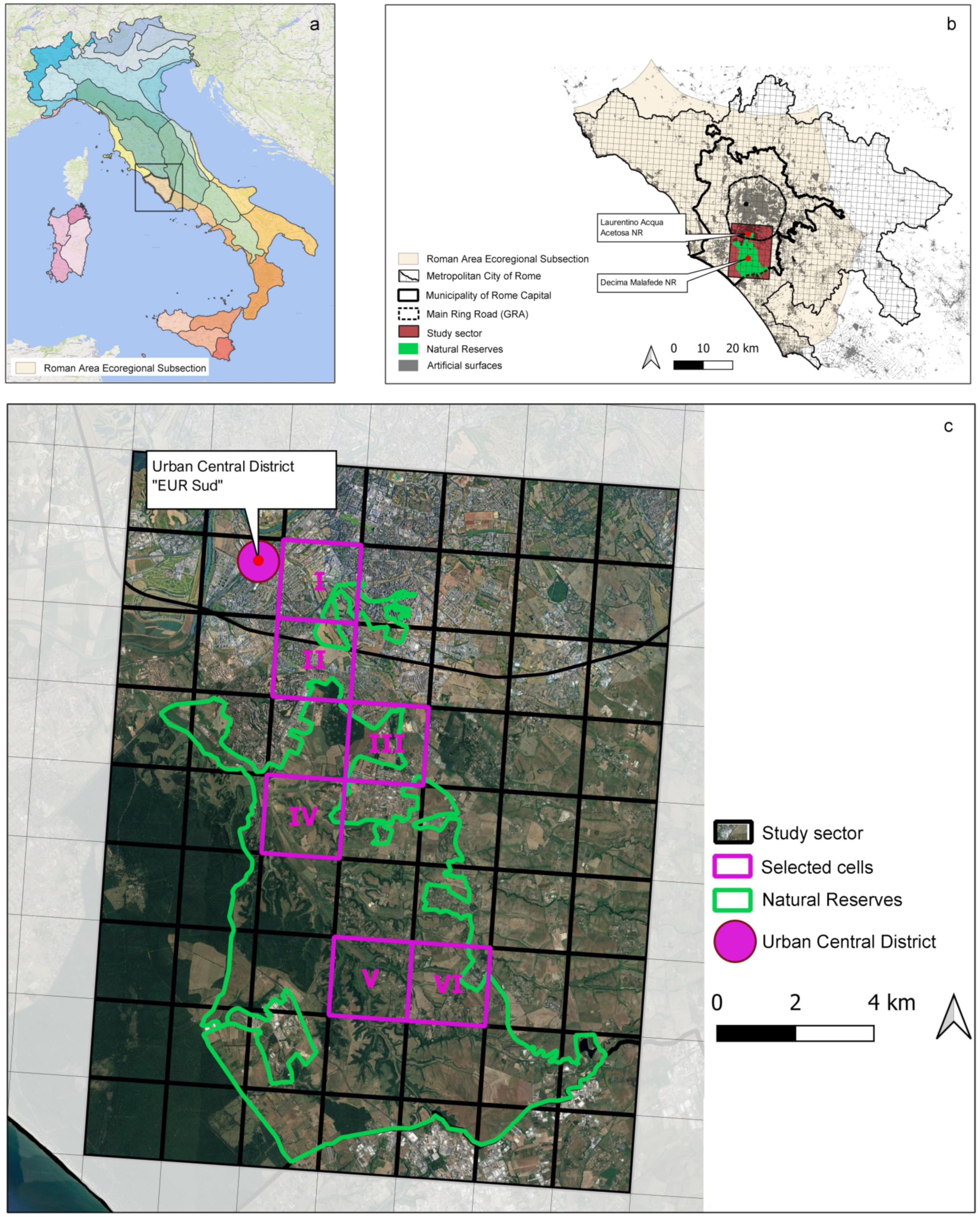
2.1. Study Area
2.2. Research Design
2.3. Input Data Collection and Compilation—Step 1
2.3.1. Actual and Potential Ecosystem Mapping—Step 1a
2.3.2. Plant and Bee Communities Field Sampling—Step 1b
2.4. Processing and Modelling—Step 2
- (i)
- measure the degree of the relationships between bee richness and diversity and the surrounding landscape mosaic, at two spatial scales, by means of statistical correlations (SC). Since bees can easily move between habitat patches even in an anthropized landscape [74,75], the correlations have been explored at both a proximal scale, within a radius of 200 m from the centroid of the sample, and a wider scale, within the whole grid cell.
- (ii)
- assess the capacity of the overall landscape mosaic to support bees, by means of MCA at the cell level.

| Indicator | Description | Modelling Phase | |
|---|---|---|---|
| Landscape Level | |||
| A | Land use/land cover proportional extent | Area of a land use/land cover class out of the total area of the grid cell or of the proximal area within a radius of 200 m (%) [based on the actual ecosystem map] | SC |
| B | Environmental unit proportional extent | Area of each EUN class out of the total area of the grid cell or of the proximal area within a radius of 200 m (%) [based on the EUN map] | SC |
| C | Linear element density | Total length of all linear elements, or of individual linear element classes, out of the total area of the grid cell or of the proximal area within a radius of 200 m (m/m2) [based on the actual ecosystem map] | SC |
| D | Environmental unit heterogeneity | Degree of EUN heterogeneity across grid cells according to Simpson and Shannon indices [76,77] [based on the EUN map] | MCA |
| E | Euclidean nearest neighbour distance (ENN) | Area-weighted average of the shortest distance between habitat patches with high value for bees (m) [78] [based on the habitat map, classes 4, 5, and 6] | MCA |
| F | Grid cell distance from the closest Urban Central District (UCD) | Spatial distance of a grid cell centre from the closest UCD adopted as a general proxy for anthropogenic pressures; according to the city masterplan [79], the closest UCD to the study area is “EUR Sud” (Km) | MCA |
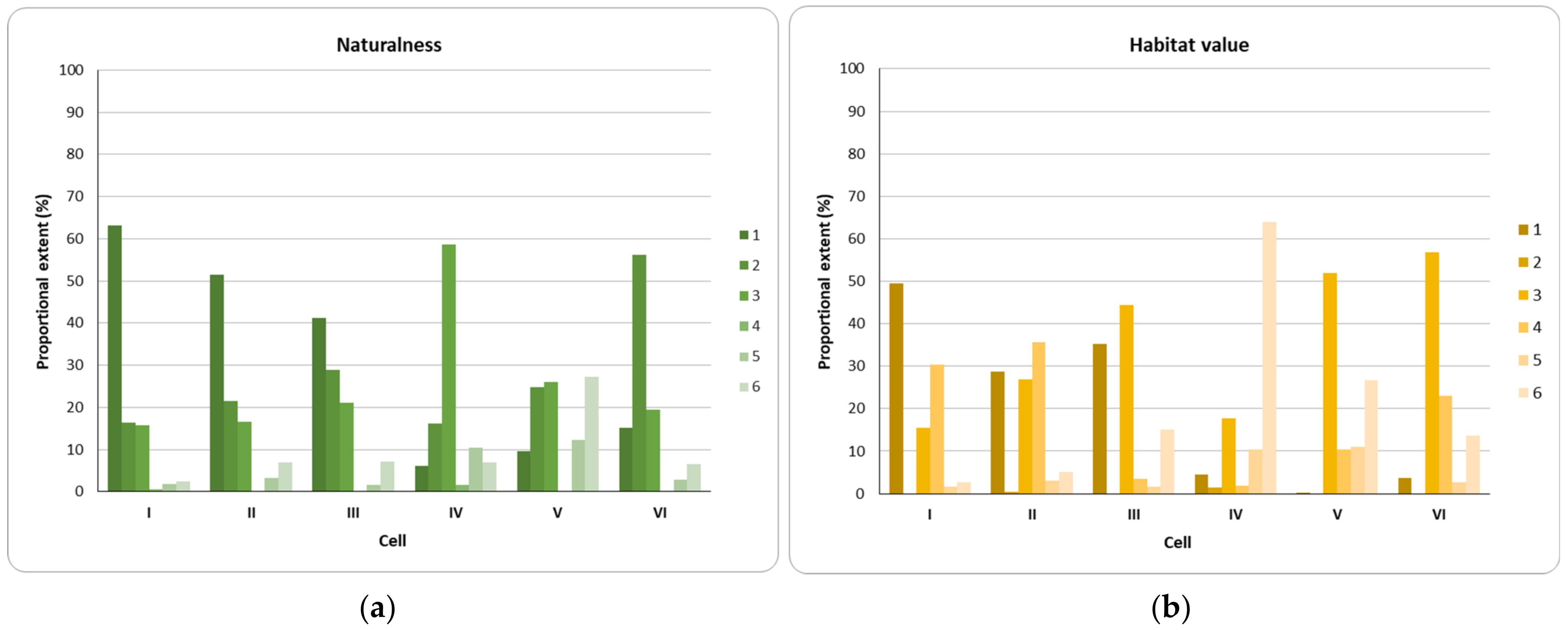
| G | Proportional extent of habitats with high value for bees | Percentage of habitat area with high value for bees out of the total area per cell (%) [based on the habitat map, classes 4, 5, and 6] | MCA |
| H | Index of landscape conservation (ILC) | Conservation status of a grid cell depending on the degree of naturalness of the land use/land cover mosaic [80] [based on the ecosystem naturalness map] | MCA |
| I | Total edge | Total length of edges between agricultural and (semi-) natural ecosystem types (km) [based on the ecosystem map simplified at the 1st level of typology] | MCA |
| L | Paved roads | Total length of paved roads (km) [based on Open Street map] | MCA |
| Habitat level | |||
| M | Proportion of blooming forbs | Non-graminoid plant species in anthesis with respect to the total plant species per sample (%) | SC |
| N | Number of blooming forbs | Total number of sampled non-graminoid plants in anthesis | MCA |
| Community level | |||
| O | Bee total abundance | Total abundance of bees per sample and per cell | SC |
| P | Bee diversity | Diversity of bee communities assessed by means of Shannon and Simpson indices. Both indices were calculated for each sample and the average value was calculated for each cell | SC |
| Q | Number of bee species | Total number of sampled bee species per cell | MCA |
2.4.1. Analysis of the Relationship between Bee Communities and Habitat/Landscape Features (SC)—Step 2a
2.4.2. Spatial Assessment of the Landscape Mosaic Capacity to Support Bees (MCA)—Step 2b
2.5. Setting of Green Infrastructure Priorities—Step 3
3. Results
3.1. Actual and Potential Ecosystem Heterogeneity—Step 1a
- “Pyroclastic plateaus” and “Gentle pyroclastic slopes” with vegetation potential for Quercus cerris and Carpinus orientalis forests (Carpino orientalis-Querceto cerridis sigmetum);
- “Steep pyroclastic slopes” and “Lithoid volcanic slopes” with vegetation potential for Quercus ilex forests (Cyclamino hederifolii-Querceto ilicis sigmetum);
- “Pyroclastic impluvia” with vegetation potential for Quercus cerris and Carpinus orientalis forests with Q. robur (Carpino orientalis-Querceto cerridis varietas quercetosum roboris sigmetum);
- “Sedimentary clayey and sandy hill plateaus” with vegetation potential for Quercus suber and Q. frainetto forests (Quercetum frainetto-suberis sigmetum);
- “Sedimentary clayey and sandy hill slopes” with vegetation potential for Quercus cerris and Q. frainetto forests (Mespilo germanicae-Querceto frainetto sigmetum);
- “Alluvial valleys” with complex vegetation potential for Quercus robur and for hygrophilous riparian forests (Fraxino-Querceto roboris, Aro italici-Alneto glutinosae, Populeto albae, and Saliceto albae sigmeta).
3.2. Bee Community Features: Abundance and Taxonomic Diversity—Step 1b
3.3. Habitat Features: Diversity and Apiarian Interest of Plant Species—Step 1b
3.4. Relationships between Bee Communities and Habitat/Landscape Features—Step 2a
3.5. Landscape Mosaic Capacity to Support Bees along the Urban-Rural Gradient—Step 2b
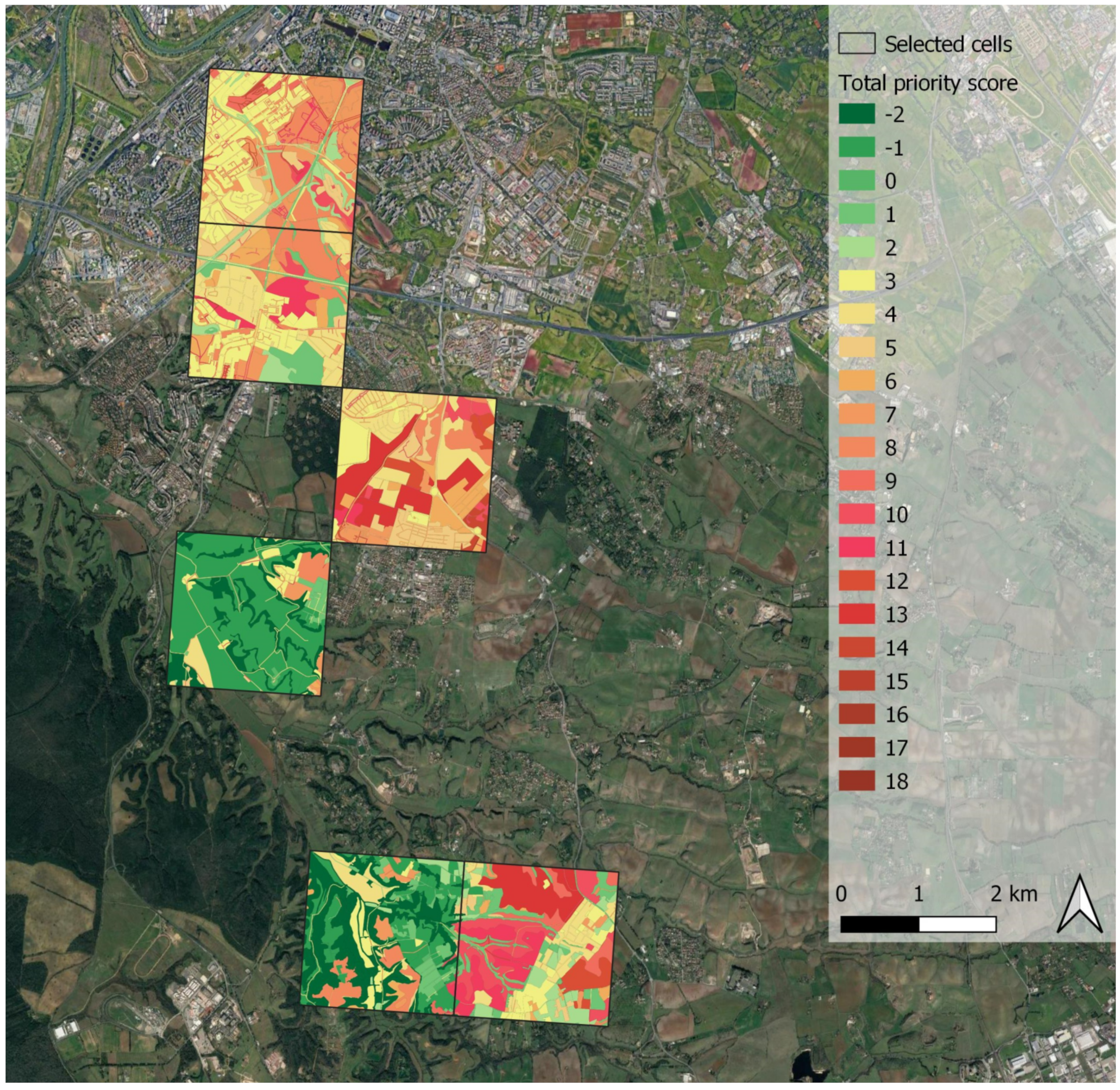
3.6. Green Infrastructure Design—Step 3
4. Discussion
5. Conclusions
Author Contributions
Funding
Data Availability Statement
Acknowledgments
Conflicts of Interest
Appendix A
| Sampled Occurrences by EUN | ||||||||
|---|---|---|---|---|---|---|---|---|
| Species | Family | AV | PI | PP | SPS | SS | GPS | LVS |
| Amegilla albigena (Lepeletier, 1841) | Apidae | x | x | |||||
| Andrena agilissima (Scopoli, 1770) | Andrenidae | x | x | |||||
| Andrena flavipes Panzer, 1799 | Andrenidae | x | x | |||||
| Andrena fuscosa Erichson, 1835 | Andrenidae | x | ||||||
| Andrena morio Brullé, 1832 | Andrenidae | x | ||||||
| Andrena pilipes Fabricius, 1781 | Andrenidae | x | x | x | x | |||
| Andrena Fabricius, 1775 | Andrenidae | x | x | |||||
| Andrena thoracica (Fabricius, 1775) | Andrenidae | x | x | |||||
| Anthidiellum strigatum (Panzer, 1804) | Megachilidae | x | ||||||
| Anthidium florentinum (Fabricius, 1775) | Megachilidae | x | x | |||||
| Anthidium manicatum (Linnaeus, 1758) | Megachilidae | x | x | x | ||||
| Apis mellifera Linnaeus, 1758 | Apidae | x | x | x | x | x | x | x |
| Bombus pascuorum (Scopoli, 1763) | Apidae | x | x | x | x | x | x | |
| Bombus ruderatus (Fabricius, 1775) | Apidae | x | x | |||||
| Bombus sylvarum (Linnaeus, 1761) | Apidae | x | ||||||
| Bombus terrestris (Linnaeus, 1758) | Apidae | x | x | x | x | |||
| Ceratina cucurbitina (Rossi, 1792) | Apidae | x | x | x | x | x | ||
| Ceratina cyanea (Kirby, 1802) | Apidae | x | ||||||
| Ceratina Latreille, 1802 | Apidae | x | x | x | x | x | ||
| Eucera clypeata Erichson, 1835 | Apidae | x | x | |||||
| Eucera nigrescens Pérez, 1879 | Apidae | x | x | x | ||||
| Eucera Scopoli, 1770 | Apidae | x | x | x | ||||
| Eucera vulpes Brullé, 1832 | Apidae | x | ||||||
| Halictus fulvipes (Klug, 1817) | Halictidae | x | ||||||
| Halictus gemmeus Dours, 1872 | Halictidae | x | x | x | x | |||
| Halictus maculatus Smith, 1848 | Halictidae | x | x | |||||
| Halictus quadricinctus (Fabricius, 1776) | Halictidae | x | x | x | ||||
| Halictus scabiosae (Rossi, 1790) | Halictidae | x | x | x | x | x | x | |
| Halictus subauratus (Rossi, 1792) | Halictidae | x | x | x | ||||
| Halictus vestitus Lepeletier, 1841 | Halictidae | x | ||||||
| Heriades crenulata Nylander, 1856 | Megachilidae | x | x | x | ||||
| Heriades truncorum (Linnaeus, 1758) | Megachilidae | x | x | |||||
| Hoplitis adunca (Panzer, 1798) | Megachilidae | x | ||||||
| Hylaeus communis Nylander, 1852 | Colletidae | x | x | x | x | x | ||
| Hylaeus Fabricius, 1793 | Colletidae | x | x | x | x | x | x | |
| Lasioglossum discum (Smith, 1853) | Halictidae | x | ||||||
| Lasioglossum leucozonium (Schrank, 1781) | Halictidae | x | x | x | ||||
| Lasioglossum malachurum (Kirby, 1802) | Halictidae | x | x | |||||
| Lasioglossum morio (Fabricius, 1793) | Halictidae | x | ||||||
| Lasioglossum nigripes (Lepeletier, 1841) | Halictidae | x | x | |||||
| Megachile albonotata Radoszkowski, 1886 | Megachilidae | x | ||||||
| Megachile apicalis Spinola, 1808 | Megachilidae | x | ||||||
| Megachile centuncularis (Linnaeus, 1758) | Megachilidae | x | ||||||
| Megachile leachella Curtis, 1828 | Megachilidae | x | ||||||
| Megachile melanopyga Costa, 1863 | Megachilidae | x | x | |||||
| Megachile rotundata (Fabricius, 1787) | Megachilidae | x | ||||||
| Megachile sculpturalis Smith, 1853 | Megachilidae | x | ||||||
| Nomada Scopoli, 1770 | Apidae | x | ||||||
| Osmia caerulescens (Linnaeus, 1758) | Megachilidae | x | ||||||
| Osmia niveata (Fabricius, 1804) | Megachilidae | x | ||||||
| Panurgus calcaratus (Scopoli, 1763) | Andrenidae | x | x | x | x | x | ||
| Pseudoanthidium scapulare (Latreille, 1809) | Megachilidae | x | ||||||
| Rhodanthidium septemdentatum (Latreille, 1809) | Megachilidae | x | ||||||
| Sphecodes Latreille, 1804 | Halictidae | x | x | |||||
| Stelis signata (Latreille, 1809) | Megachilidae | x | x | |||||
| Systropha curvicornis (Scopoli, 1770) | Halictidae | x | x | |||||
| Xylocopa iris (Christ, 1791) | Apidae | x | x | |||||
| Xylocopa violacea (Linnaeus, 1758) | Apidae | x | x | x | ||||
Appendix B
| Sampled Occurrences by EUN | ||||||||
|---|---|---|---|---|---|---|---|---|
| Species Name | Family | AV | PI | PP | SPS | SS | GPS | LVS |
| Acer campestre L. | Sapindaceae | x | ||||||
| Ailanthus altissima (Mill.) Swingle [N] | Simaroubaceae | x | x | x | ||||
| Ajuga iva (L.) Schreb. subsp. iva | Lamiaceae | x | ||||||
| Allium polyanthum Schult. & Schult. f. | Amaryllidaceae | x | ||||||
| Alnus glutinosa (L.) Gaertn. | Betulaceae | x | x | |||||
| Anchusa undulata subsp. hybrida (Ten.) Bég. | Boraginaceae | x | x | x | x | x | ||
| Anthemis arvensis L. subsp. arvensis | Asteraceae | x | ||||||
| Antirrhinum majus L. subsp. majus [A] | Plantaginaceae | x | ||||||
| Arctium lappa L. | Asteraceae | x | ||||||
| Artemisia vulgaris L. | Asteraceae | x | x | |||||
| Arum maculatum L. | Araceae | x | ||||||
| Asparagus acutifolius L. | Asparagaceae | x | x | x | x | |||
| Asphodelus ramosus L. subsp. ramosus var. ramosus | Xanthorrhoeaceae | x | ||||||
| Ballota nigra L. subsp. meridionalis (Bég.) Bég. | Lamiaceae | x | x | |||||
| Borago officinalis L. | Boraginaceae | x | x | x | x | x | x | |
| Brassica nigra (L.) W.D.J. Koch [D] | Brassicaceae | x | ||||||
| Calamintha nepeta (L.) Savi subsp. glandulosa P.W. Ball (Req.) | Lamiaceae | x | x | x | x | x | x | |
| Calystegia sepium (L.) R. Br. subsp. sepium | Convolvulaceae | x | x | x | ||||
| Campanula rapunculus L. | Campanulaceae | x | ||||||
| Capsella bursa-pastoris (L.) Medik. subsp. bursa-pastoris | Brassicaceae | x | ||||||
| Carduus nutans L. subsp. nutans | Asteraceae | x | ||||||
| Carduus pycnocephalus L. subsp. pycnocephalus | Asteraceae | x | ||||||
| Carlina corymbosa L. | Asteraceae | x | ||||||
| Carthamus lanatus L. subsp. lanatus | Asteraceae | x | x | |||||
| Celtis australis L. subsp. australis | Cannabaceae | x | ||||||
| Centaurea calcitrapa L. | Asteraceae | x | ||||||
| Centaurea napifolia L. | Asteraceae | x | ||||||
| Centaurea solstitialis L. subsp. solstitialis | Asteraceae | x | x | x | ||||
| Chenopodium album L. | Amaranthaceae | x | x | x | x | x | x | x |
| Chenopodium strictum Roth subsp. strictum | Amaranthaceae | x | ||||||
| Cichorium intybus L. subsp. intybus | Asteraceae | x | x | x | x | x | x | x |
| Cirsium arvense (L.) Scop. | Asteraceae | x | ||||||
| Cirsium vulgare (Savi) Ten. | Asteraceae | x | x | x | x | x | ||
| Clematis vitalba L. | Ranunculaceae | x | x | x | x | x | x | |
| Convolvulus althaeoides L. | Convolvulaceae | x | ||||||
| Convolvulus arvensis L. | Convolvulaceae | x | x | x | x | x | x | x |
| Convolvulus cantabrica L. | Convolvulaceae | x | x | |||||
| Crataegus monogyna Jacq. subsp. monogyna | Rosaceae | x | ||||||
| Crepis neglecta L. | Asteraceae | x | ||||||
| Crepis setosa Haller f. | Asteraceae | x | x | x | x | x | ||
| Cynoglossum creticum Mill. | Boraginaceae | x | ||||||
| Cynoglossum officinale L. | Boraginaceae | x | x | |||||
| Cyperus longus L. | Cyperaceae | x | ||||||
| Cytisus villosus Pourr. | Fabaceae | x | ||||||
| Daucus carota L. subsp. carota | Apiaceae | x | x | x | x | x | x | x |
| Delphinium halteratum Sm. subsp. halteratum | Ranunculaceae | x | x | x | ||||
| Diplotaxis muralis (L.) DC. | Brassicaceae | x | ||||||
| Dipsacus fullonum L. | Caprifoliaceae | x | x | |||||
| Echium italicum L. subsp. italicum | Boraginaceae | x | x | x | x | x | ||
| Echium plantagineum L. | Boraginaceae | x | x | x | x | x | x | |
| Echium vulgare L. | Boraginaceae | x | ||||||
| Epilobium hirsutum L. | Onagraceae | x | ||||||
| Epilobium lanceolatum Sebast. et Mauri | Onagraceae | x | ||||||
| Epilobium tetragonum L. subsp. tetragonum | Onagraceae | x | x | |||||
| Eruca vesicaria (L.) Cav. | Brassicaceae | x | ||||||
| Eryngium maritimum L. | Apiaceae | x | x | x | ||||
| Eucalyptus globulus Labill. [N] | Myrtaceae | x | ||||||
| Euonymus europaeus L. | Celastraceae | x | x | x | x | x | ||
| Foeniculum vulgare Mill. subsp. vulgare | Apiaceae | x | x | x | x | x | x | x |
| Galega officinalis L. | Fabaceae | x | ||||||
| Galium album Mill. | Rubiaceae | x | x | x | ||||
| Galium aparine L. | Rubiaceae | x | x | x | x | x | x | x |
| Geranium molle L. | Geraniaceae | x | ||||||
| Hedera helix L. subsp. helix | Araliaceae | x | x | x | x | x | ||
| Hypericum perforatum L. | Hypericaceae | x | x | x | x | x | ||
| Juglans regia L. [C] | Juglandaceae | x | x | |||||
| Knautia arvensis (L.) Coult. | Caprifoliaceae | x | x | x | ||||
| Knautia integrifolia (L.) Bertol. subsp. integrifolia | Caprifoliaceae | x | x | x | x | x | ||
| Lathyrus annuus L. | Fabaceae | x | ||||||
| Laurus nobilis L. | Lauraceae | x | x | x | ||||
| Lavatera cretica L. | Malvaceae | x | ||||||
| Linaria pelisseriana (L.) Mill. | Plantaginaceae | x | ||||||
| Linaria purpurea (L.) Mill. | Plantaginaceae | x | x | |||||
| Linaria vulgaris Mill. subsp. vulgaris | Plantaginaceae | x | x | x | x | x | x | |
| Lythrum salicaria L. | Lythraceae | x | ||||||
| Malva arborea (L.) Webb & Berthel. | Malvaceae | x | ||||||
| Malva sylvestris L. subsp. sylvestris | Malvaceae | x | x | x | x | x | x | |
| Medicago sativa L. [D] | Fabaceae | x | x | x | x | x | x | x |
| Melilotus albus Medik. | Fabaceae | x | ||||||
| Mentha suaveolens Ehrh. subsp. suaveolens | Lamiaceae | x | ||||||
| Nigella damascena L. | Ranunculaceae | x | x | |||||
| Olea europaea L. [C] | Oleaceae | x | ||||||
| Oxalis corniculata L. | Oxalidaceae | x | x | |||||
| Oxalis stricta L. [N] | Oxalidaceae | x | ||||||
| Papaver rhoeas L. subsp. rhoeas [D] | Papaveraceae | x | x | x | x | x | x | x |
| Petasites hybridus (L.) P. Gaertn., B. Mey. et Scherb | Asteraceae | x | ||||||
| Picris echioides L. | Asteraceae | x | x | x | x | x | ||
| Picris hieracioides L. subsp. hieracioides | Asteraceae | x | x | x | x | x | x | x |
| Plantago lanceolata L. | Plantaginaceae | x | x | x | x | |||
| Plantago major L. subsp. major | Plantaginaceae | x | x | |||||
| Polygonum arenastrum Boreau subsp. arenastrum | Polygonaceae | x | x | x | ||||
| Populus nigra L. | Salicaceae | x | ||||||
| Portulaca oleracea L. subsp. oleracea | Portulacaceae | x | x | |||||
| Prunus cerasifera Ehrh. [A] | Rosaceae | x | ||||||
| Prunus spinosa L. subsp. spinosa | Rosaceae | x | x | x | x | x | x | |
| Pyrus pyraster Burgsd. | Rosaceae | x | x | x | ||||
| Quercus ilex L. subsp. ilex | Fagaceae | x | ||||||
| Quercus robur L. subsp. robur | Fagaceae | x | ||||||
| Quercus suber L. | Fagaceae | x | x | x | ||||
| Quercus virgiliana (Ten.) Ten. | Fagaceae | x | x | x | x | x | ||
| Raphanus raphanistrum L. subsp. raphanistrum | Brassicaceae | x | x | x | x | x | x | x |
| Reseda phyteuma L. subsp. phyteuma | Resedaceae | x | x | |||||
| Robinia pseudacacia L. [N] | Fabaceae | x | x | x | ||||
| Rosa canina L. | Rosaceae | x | x | |||||
| Rosa sempervirens L. | Rosaceae | x | x | x | x | |||
| Rubus ulmifolius Schott | Rosaceae | x | x | x | x | x | x | x |
| Rumex acetosa L. subsp. acetosa | Polygonaceae | x | ||||||
| Rumex acetosella L. subsp. pyrenaicus (Pourr. ex Lapeyr.) Akeroyd | Polygonaceae | x | ||||||
| Rumex aquaticus L. | Polygonaceae | x | ||||||
| Rumex bucephalophorus L. subsp. bucephalophorus | Polygonaceae | x | x | x | x | x | ||
| Rumex conglomeratus Murray | x | x | x | x | ||||
| Rumex crispus L. | Polygonaceae | x | x | x | x | x | ||
| Rumex obtusifolius L. subsp. obtusifolius | Polygonaceae | x | x | x | x | x | ||
| Rumex pulcher L. subsp. pulcher | Polygonaceae | x | x | |||||
| Rumex sanguineus L. | Polygonaceae | x | x | x | x | |||
| Salix alba L. subsp. alba | Salicaceae | x | x | |||||
| Salix triandra L. subsp. amygdalyna (L.) Schübl. et G. Martens | Salicaceae | x | x | |||||
| Salvia verbenaca L. | Lamiaceae | |||||||
| Sambucus ebulus L. | Adoxaceae | x | ||||||
| Sambucus nigra L. | Adoxaceae | x | x | x | x | x | ||
| Sanguisorba minor Scop. subsp. balearica (Bourg. ex Nyman) Muñoz Garm. et C. Navarro | Rosaceae | x | ||||||
| Scabiosa columbaria L. | Caprifoliaceae | x | x | |||||
| Scabiosa maritima L. | Caprifoliaceae | x | x | |||||
| Senecio erraticus Bertol. subsp. erraticus | Asteraceae | x | x | x | x | x | ||
| Senecio vulgaris L. | Asteraceae | x | x | |||||
| Silene alba (Mill.) E. H. L. Krause | Caryophyllaceae | x | ||||||
| Silene laeta (Aiton) Godr. | Caryophyllaceae | x | x | x | x | x | x | x |
| Silybum marianum (L.) Gaertn. | Asteraceae | x | ||||||
| Sinapis arvensis L. subsp. arvensis | Brassicaceae | x | x | x | x | x | x | x |
| Stachys arvensis (L.) L. | Lamiaceae | x | x | x | ||||
| Stachys germanica L. subsp. germanica | Lamiaceae | x | ||||||
| Stachys ocymastrum (L.) Briq. | Lamiaceae | x | ||||||
| Stachys sylvatica L. | Lamiaceae | x | ||||||
| Taraxacum megalorrhizon (Forssk.) Hand. -Mazz. | Asteraceae | x | x | x | ||||
| Tordylium maximum L. | Apiaceae | x | x | |||||
| Trifolium angustifolium L. subsp. angustifolium | Fabaceae | x | x | x | ||||
| Trifolium campestre Schreb. | Fabaceae | x | x | x | ||||
| Trifolium incarnatum L. subsp. incarnatum [C] | Fabaceae | x | x | x | x | |||
| Trifolium pallidum Waldst. et Kit. | Fabaceae | x | ||||||
| Trifolium pratense L. subsp. pratense | Fabaceae | x | x | x | x | x | ||
| Trifolium repens L. subsp. repens | Fabaceae | x | ||||||
| Trifolium sebastianii Savi | Fabaceae | x | ||||||
| Trifolium squarrosum L. | Fabaceae | x | ||||||
| Trigonella alba (Medik.) Coulot & Rabaute | Fabaceae | x | ||||||
| Ulmus minor Mill. subsp. minor | Fabaceae | x | x | x | x | x | x | x |
| Urospermum picroides (L.) Scop. ex F.W. Schmidt | Asteraceae | x | ||||||
| Verbascum blattaria L. | Scrophulariaceae | x | x | x | x | |||
| Verbascum pulverulentum Vill. | Scrophulariaceae | x | ||||||
| Verbascum sinuatum L. | Scrophulariaceae | x | x | x | x | x | x | x |
| Verbascum thapsus L. subsp. thapsus | Scrophulariaceae | x | x | |||||
| Verbena officinalis L. | Verbenaceae | x | x | x | x | x | ||
| Veronica arvensis L. | Plantaginaceae | x | ||||||
| Veronica persica Poir. [N] | Plantaginaceae | x | ||||||
| Vicia cracca L. | Fabaceae | x | x | x | x | |||
| Vicia villosa Roth subsp. varia (Host) Corb. | Fabaceae | x | x | x | x | |||
| Viola tricolor L. subsp. tricolor | Violaceae | x | ||||||
| Vitis vinifera L. [C] | Vitaceae | x | x | x | ||||
| Xanthium italicum Moretti | Asteraceae | x | x | |||||
| Xanthium spinosum L. [N] | Asteraceae | x | x | |||||
References
- Kleijn, D.; Winfree, R.; Bartomeus, I.; Carvalheiro, L.G.; Henry, M.; Isaacs, R.; Klein, A.-M.; Kremen, C.; M’Gonigle, L.K.; Rader, R.; et al. Delivery of crop pollination services is an insufficient argument for wild pollinator conservation. Nat. Commun. 2015, 6, 7414. [Google Scholar] [CrossRef] [PubMed] [Green Version]
- Senapathi, D.; Biesmeijer, J.C.; Breeze, T.D.; Kleijn, D.; Potts, S.G.; Carvalheiro, L.G. Pollinator conservation—The difference between managing for pollination services and preserving pollinator diversity. Curr. Opin. Insect Sci. 2015, 12, 93–101. [Google Scholar] [CrossRef] [Green Version]
- Potts, S.G.; Imperatriz-Fonseca, V.; Ngo, H.T.; Aizen, M.A.; Biesmeijer, J.C.; Breeze, T.D.; Dicks, L.V.; Garibaldi, L.A.; Hill, R.; Settele, J.; et al. Safeguarding pollinators and their values to human well-being. Nature 2016, 540, 220–229. [Google Scholar] [CrossRef] [PubMed] [Green Version]
- Bartholomée, O.; Lavorel, S. Disentangling the diversity of definitions for the pollination ecosystem service and associated estimation methods. Ecol. Indic. 2019, 107, 105576. [Google Scholar] [CrossRef]
- Hristov, P.; Neov, B.; Shumkova, R.; Palova, N. Significance of Apoidea as Main Pollinators. Ecological and Economic Impact and Implications for Human Nutrition. Diversity 2020, 12, 280. [Google Scholar] [CrossRef]
- Zulian, G.; Maes, J.; Paracchini, M.L. Linking Land Cover Data and Crop Yields for Mapping and Assessment of Pollination Services in Europe. Land 2013, 2, 472–492. [Google Scholar] [CrossRef] [Green Version]
- Capriolo, A.; Boschetto, R.G.; Mascolo, R.A.; Balbi, S.; Villa, F. Biophysical and economic assessment of four ecosystem services for natural capital accounting in Italy. Ecosyst. Serv. 2020, 46, 101207. [Google Scholar] [CrossRef]
- Porto, R.G.; de Almeida, R.F.; Cruz-Neto, O.; Tabarelli, M.; Viana, B.F.; Peres, C.A.; Lopes, A.V. Pollination Ecosystem Services: A Comprehensive Review of Economic Values, Research Funding and Policy Actions. Food Secur. 2020, 12, 1425–1442. [Google Scholar] [CrossRef]
- Jordan, A.; Patch, H.M.; Grozinger, C.M.; Khanna, V. Economic Dependence and Vulnerability of United States Agricultural Sector on Insect-Mediated Pollination Service. Environ. Sci. Technol. 2021, 55, 2243–2253. [Google Scholar] [CrossRef]
- Zattara, E.E.; Aizen, M.A. Worldwide occurrence records suggest a global decline in bee species richness. One Earth 2021, 4, 114–123. [Google Scholar] [CrossRef]
- EC (European Commission). EU Biodiversity Strategy for 2030-Bringing Nature Back into Our Lives; Communication from the Commission to the European Parliament, the Council, the European Economic and Social Committee and the Committee of the Regions COM. 2020. Available online: https://eur-lex.europa.eu/legal-content/EN/TXT/?qid=1590574123338&uri=CELEX:52020DC0380 (accessed on 7 November 2021).
- DEFRA (Department for Environment, Food and Rural Affairs). National Pollinator Strategy: Implementation Plan, 2018–2202. 2018. Available online: https://www.gov.uk/search/all (accessed on 7 November 2021).
- Gemmill-Herren, B.; Garibaldi, L.A.; Kremen, C.; Ngo, H.T. Building Effective Policies to Conserve Pollinators: Translating Knowledge into Policy. Curr. Opin. Insect Sci. 2021, 46, 64–71. [Google Scholar] [CrossRef]
- IEEP (Institute for European Environmental Policy). Pollinator Initiatives in EU Member States: Success Factors and Gaps. 2017. Available online: https://ieep.eu/ (accessed on 7 November 2021).
- EC (European Commission). EU Pollinators Initiative; Communication from the Commission to the European Parliament, the Council, the European Economic and Social Committee and the Committee of the Regions COM. 2018. Available online: https://ec.europa.eu/environment/nature/conservation/species/pollinators/policy_en.htm (accessed on 7 November 2021).
- Vanbergen, A.J.; Initiative, T.I.P. Threats to an ecosystem service: Pressures on pollinators. Front. Ecol. Environ. 2013, 11, 251–259. [Google Scholar] [CrossRef] [Green Version]
- Woodcock, B.A.; Bullock, J.M.; Shore, R.F.; Heard, M.S.; Pereira, M.G.; Redhead, J.; Ridding, L.; Dean, H.; Sleep, D.; Henrys, P.; et al. Country-specific effects of neonicotinoid pesticides on honey bees and wild bees. Science 2017, 356, 1393–1395. [Google Scholar] [CrossRef] [Green Version]
- Mathiasson, M.E.; Rehan, S.M. Wild bee declines linked to plant-pollinator network changes and plant species introductions. Insect Conserv. Divers. 2020, 13, 595–605. [Google Scholar] [CrossRef]
- Ollerton, J.; Erenler, H.; Edwards, M.; Crockett, R. Pollinator declines. Extinctions of aculeate pollinators in Britain and the role of large-scale agricultural changes. Science 2014, 346, 1360–1362. [Google Scholar] [CrossRef] [Green Version]
- Buchholz, S.; Kowarik, I. Urbanisation modulates plant-pollinator interactions in invasive vs. native plant species. Sci. Rep. 2019, 9, 6375. [Google Scholar] [CrossRef] [Green Version]
- ECA (European Court of Auditors). Protection of Wild Pollinators in the EU—Commission Initiatives Have Not Borne Fruit. 2020. Available online: https://www.eca.europa.eu/en/Pages/DocItem.aspx?did=54200 (accessed on 7 November 2021).
- Thimmegowda, G.G.; Mullen, S.; Sottilare, K.; Sharma, A.; Mohanta, S.S.; Brockmann, A.; Dhandapany, P.S.; Olsson, S.B. A field–based quantitative analysis of sublethal effects of air pollution on pollinators. Proc. Natl. Acad. Sci. USA 2020, 117, 20653–20661. [Google Scholar] [CrossRef]
- Wenzel, A.; Grass, I.; Belavadi, V.V.; Tscharntke, T. How Urbanization is Driving Pollinator Diversity and Pollination–A Systematic Review. Biol. Conserv. 2020, 241, 108321. [Google Scholar] [CrossRef]
- Tommassi, P.; Miro, A.; Higo, H.A.; Winston, M. Bee diversity and abundance in a urban setting. Can. Enthomol. 2004, 136, 851–869. [Google Scholar] [CrossRef]
- Matteson, K.C.; Langellotto, G.A. Small scale additions of native plants fail to increase beneficial insect richness in urban gardens. Insect Conserv. Divers. 2011, 4, 89–98. [Google Scholar] [CrossRef]
- Stange, E.; Zulian, G.; Rusch, G.; Barton, D.; Nowell, M. Ecosystem services mapping for municipal policy: ESTIMAP and zoning for urban beekeeping. One Ecosyst. 2017, 2, e14014. [Google Scholar] [CrossRef] [Green Version]
- Wania, A.; Kuhn, I.; Klotz, S. Plant richness patterns in agricultural and urban landscapes in Central Germany—Spatial gradients of species richness. Landsc. Urban Plan. 2006, 75, 97–110. [Google Scholar] [CrossRef]
- Capotorti, G.; Del Vico, E.; Lattanzi, E.; Tilia, A.; Celesti-Grapow, L. Exploring biodiversity in a metropolitan area in the Mediterranean region: The urban and suburban flora of Rome (Italy). Plant Biosyst. 2013, 147, 174–185. [Google Scholar] [CrossRef]
- Baldock, K.C.R.; Goddard, M.A.; Hicks, D.M.; Kunin, W.E.; Mitschunas, N.; Osgathorpe, L.M.; Potts, S.G.; Robertson, K.M.; Scott, A.V.; Stone, G.N.; et al. Where is the UK’s pollinator biodiversity? The importance of urban areas for flower-visiting insects. Proc. R. Soc. B Biol. Sci. 2015, 282, 20142849. [Google Scholar] [CrossRef] [PubMed] [Green Version]
- Kaluza, B.F.; Wallace, H.; Heard, T.A.; Klein, A.-M.; Leonhardt, S.D. Urban gardens promote bee foraging over natural habitats and plantations. Ecol. Evol. 2016, 6, 1304–1316. [Google Scholar] [CrossRef] [PubMed] [Green Version]
- Hall, D.M.; Camilo, G.R.; Tonietto, R.K.; Ollerton, J.; Ahrné, K.; Arduser, M.; Ascher, J.S.; Baldock, K.C.; Fowler, R.; Frankie, G.; et al. The city as a refuge for insect pollinators. Conserv. Biol. 2017, 31, 24–29. [Google Scholar] [CrossRef] [Green Version]
- Hostetler, M.E.; McIntyre, N.E. Effects of urban land use on pollinator (Hymenoptera: Apoidea) communities in a desert metropolis. Basic Appl. Ecol. 2001, 2, 209–218. [Google Scholar] [CrossRef] [Green Version]
- Casiker, C.V.; Jagadishakumara, B.; Sunil, G.M.; Chaithra, K.; Devy, M.S. Bee Diversity in the Rural–Urban Interface of Bengaluru and Scope for Pollinator-Integrated Urban Agriculture. In The Rural-Urban Interface: Bee Diversity in the Rural–Urban Interface of Bengaluru and Scope for Pollinator-Integrated Urban Agriculture; Hoffmann, E., Buerkert, A., von Cramon-Taubadel, S., Umesh, K.B., Pethandlahalli Shivaraj, P., Vazhacharickal, P.J., Eds.; Springer: Berlin, Germany, 2021; pp. 171–182. [Google Scholar]
- Moore, L.J.; Kosut, M. Buzz: Urban Beekeeping and the Power of the Bee; New York University Press: New York, NY, USA; London, UK, 2013. [Google Scholar]
- Gunnarsson, B.; Federsel, L.M. Bumblebees in the city: Abundance, Species Richness and Diversity in Two Urban Habitats. J. Insect Conserv. 2014, 18, 1185–1191. [Google Scholar] [CrossRef] [Green Version]
- Fukase, J.; Simons, A. Increased pollinator activity in urban gardens with more native flora. Appl. Ecol. Environ. Res. 2016, 14, 297–310. [Google Scholar] [CrossRef]
- Daniels, B.; Jedamski, J.; Ottermanns, R.; Ross-Nickoll, M. A “plan bee” for cities: Pollinator diversity and plant-pollinator interactions in urban green spaces. PLoS ONE 2020, 15, e0235492. [Google Scholar] [CrossRef]
- Pufal, G.; Steffan-Dewenter, I.; Klein, A.-M. Crop pollination services at the landscape scale. Curr. Opin. Insect Sci. 2017, 21, 91–97. [Google Scholar] [CrossRef]
- EC (European Commission). Review of Progress on Implementation of the EU Green Infrastructure Strategy; Report from the Commission to the European Parliament, the Council, the European Economic and Social Committee and the Committee of the Regions COM. 2019. Available online: https://ec.europa.eu/environment/nature/ecosystems/index_en.htm (accessed on 7 November 2021).
- Banaszak-Cibicka, W.; Ratyńska, H.; Dylewski, L. Features of urban green space favourable for large and diverse bee populations (Hymenoptera: Apoidea: Apiformes). Urban For. Urban Green. 2016, 20, 448–452. [Google Scholar] [CrossRef]
- Gren, A.; Andersson, E. Being efficient and green by rethinking the urban-rural divide—Combining urban expansion and food production by integrating an ecosystem service perspective into urban planning. Sustain. Cities Soc. 2018, 40, 75–82. [Google Scholar] [CrossRef]
- Langellotto, G.; Melathopoulos, A.; Messer, I.; Anderson, A.; McClintock, N.; Costner, L. Garden pollinators and the potential for ecosystem service flow to urban and peri-urban agriculture. Sustainability 2018, 10, 2047. [Google Scholar] [CrossRef] [Green Version]
- Turo, K.J.; Spring, M.R.; Sivakoff, F.S.; De La Flor, Y.A.D.; Gardiner, M.M. Conservation in post-industrial cities: How does vacant land management and landscape configuration influence urban bees? J. Appl. Ecol. 2021, 58, 58–69. [Google Scholar] [CrossRef]
- Bonifazi, A.; Balena, P.; Rega, C. Pollination and the Integration of Ecosystem Services in Landscape Planning and Rural Development. In Lecture Notes in Computer Science: Computational Science and Its Applications—ICCSA 2017; Part V; Gervasi, O., Ed.; ICCSA: Trieste, Italy, 2017; pp. 118–133. [Google Scholar]
- Rega, C.; Bartual, A.M.; Bocci, G.; Sutter, L.; Albrecht, M.; Moonen, A.C.; Jeanneret, P.; van der Werf, W.; Pfister, S.C.; Holland, J.M.; et al. A pan-European model of landscape potential to support natural pest control services. Ecol. Indic. 2018, 90, 653–664. [Google Scholar] [CrossRef]
- Bates, A.J.; Sadler, J.P.; Fairbrass, A.J.; Falk, S.J.; Hale, J.D.; Matthews, T.J. Changing bee and hoverfly pollinator assemblages along an urban-rural gradient. PLoS ONE 2011, 6, e23459. [Google Scholar] [CrossRef]
- Biella, P.; Tommasi, N.; Guzzetti, L.; Pioltelli, E.; Labra, M.; Galimberti, A. City climate and landscape structure shape pollinators, nectar and transported pollen along a gradient of urbanization. J. Appl. Ecol. 2022, 59, 1586–1595. [Google Scholar] [CrossRef]
- Funiciello, R.; Giordano, G.; Mattei, M. Carta Geologica del Comune di Roma/Geological Map of the Municipality of Roma (1:50000). 2008. Available online: https://www.isprambiente.gov.it/it/pubblicazioni/periodici-tecnici/memorie-descrittive-della-carta-geologica-ditalia/la-geologia-di-roma-dal-centro-storico-alla (accessed on 7 November 2021).
- Blasi, C.; Capotorti, G.; Copiz, R.; Guida, D.; Mollo, B.; Smiraglia, D.; Zavattero, L. Classification and mapping of the ecoregions of Italy. Plant Biosyst. 2014, 148, 1255–1345. [Google Scholar] [CrossRef]
- Blasi, C.; Capotorti, G.; Copiz, R.; Mollo, B. A first revision of the Italian Ecoregion map. Plant Biosyst. 2018, 152, 1201–1204. [Google Scholar] [CrossRef]
- Frondoni, R.; Mollo, B.; Capotorti, G. A landscape analysis of land cover change in the Municipality of Rome (Italy): Spatio-temporal characteristics and ecological implications of land cover transitions from 1954 to 2001. Landsc. Urban Plan. 2011, 100, 117–128. [Google Scholar] [CrossRef]
- Provincia di Roma, Piano Territoriale Provinciale Generale. Rapporto Territorio: Sistema della Mobilità. 2015. Available online: http://ptpg.cittametropolitanaroma.gov.it/UploadDocs/2010/rapporto_territorio/ (accessed on 7 November 2021).
- Blasi, C.; Capotorti, G.; Alós Ortí, M.M.; Anzellotti, I.; Attorre, F.; Azzella, M.M.; Carli, E.; Copiz, R.; Garfì, V.; Manes, F.; et al. Ecosystem mapping for the implementation of the European Biodiversity Strategy at the national level: The case of Italy. Environ. Sci. Policy 2017, 78, 173–184. [Google Scholar] [CrossRef]
- Weiss, M.; Banko, G. Ecosystem Type Map v3.1—Terrestrial and Marine Ecosystems; EEA-European Topic Centre on Biological Diversity: Paris, France, 2018. [Google Scholar]
- Blasi, C.; Capotorti, G.; Frondoni, R. Defining and mapping typological models at the landscape scale. Plant Biosyst. 2005, 139, 155–163. [Google Scholar] [CrossRef]
- Tüxen, R. Die Heutige Potentielle Natürliche Vegetation Als Gegenstand der Vegetationskartierung; Zentralstelle für Vegetationskartierung: Remagen, Germany, 1956. [Google Scholar]
- Loidi, J.; Fernandez-Gonzalez, F. Potential natural vegetation: Reburying or reboring? J. Veg. Sci. 2012, 23, 596–604. [Google Scholar] [CrossRef]
- CIRBFEP (Centro di Ricerca Interuniversitario Biodiversità, Fitosociologia ed Ecologia del Paesaggio). Carta della Vegetazione reale della Provincia di Roma. 2013. Available online: http://websit.cittametropolitanaroma.it/BDV2014/Veget_Reale.aspx (accessed on 7 November 2021).
- Phillips, B.B.; Bullock, J.M.; Osborne, J.L.; Gaston, K.J.; Manning, P. Ecosystem service provision by road verges. J. Appl. Ecol. 2020, 7, 488–501. [Google Scholar] [CrossRef]
- Capotorti, G.; Guida, D.; Siervo, V.; Smiraglia, D.; Blasi, C. Ecological classification of land and conservation of biodiversity at the national level: The case of Italy. Biol. Conserv. 2012, 147, 174–183. [Google Scholar] [CrossRef]
- Capotorti, G.; Zavattero, L.; Anzellotti, I.; Burrascano, S.; Frondoni, R.; Marchetti, M.; Marignani, M.; Smiraglia, D.; Blasi, C. Do National Parks play an active role in conserving the natural capital of Italy? Plant Biosyst. 2012, 146, 258–265. [Google Scholar] [CrossRef]
- Ricciardelli D’Albore, G.; Persano Oddo, L. Flora Apistica Italiana, 1st ed.; Istituto Sperimentale per la Zoologia Agraria: Firenze, Italy, 1981. [Google Scholar]
- Persano Oddo, L. Mieli e flora mellifera del Lazio; Produced as part of the “Programma finalizzato al miglioramento della produzione e commercializzazione del miele”—Piano di attuazione Sottoprogramma operativo Regione Lazio—Annualità 2005–2006; Istituto Zooprofilattico Sperimentale delle Regioni Lazio e Toscana: Pisa, Italy, 2006. [Google Scholar]
- Hopwood, J.L. The contribution of roadside grassland restorations to native bee conservation. Biol. Conserv. 2008, 141, 2632–2640. [Google Scholar] [CrossRef]
- Blasi, C.; Canini, L.; Capotorti, G.; Celesti, L.; Del Moro, M.A.; Ercole, S.; Filesi, L.; Fiorini, S.; Lattanzi, E.; Leoni, G.; et al. Flora, vegetazione ed ecologia del paesaggio delle aree protette di RomaNatura. Inf. Bot. Ital. 2001, 33, 14–18. [Google Scholar]
- Blasi, C.; Capotorti, G. Carta Delle Serie di Vegetazione del Territorio del Comune di Roma (1:50,000). 2007. Available online: http://www.urbanistica.comune.roma.it (accessed on 7 November 2021).
- Waddington, K.D.; Holden, L.R. Optimal foraging: On flower selection by bees. Am. Nat. 1979, 114, 179–196. [Google Scholar] [CrossRef]
- Gumbert, A.; Kunze, J. Inflorescence height affects visitation behavior of bees-a case study of an aquatic plant community in bolivia. Biotropica 1999, 31, 466–477. [Google Scholar] [CrossRef]
- Cane, J.H.; Minckley, R.L.; Kervin, L.J. Sampling bees (Hymenoptera: Apiformes) for pollinator community studies: Pitfalls of pan trapping. J. Kans. Entomol. Soc. 2000, 73, 225–231. [Google Scholar]
- Integrated Taxonomic Information System (ITIS). 2023. Available online: https://www.itis.gov/ (accessed on 25 January 2023).
- Westhoff, V.; Van Der Maarel, E. The braun-blanquet approach. In Classification of Plant Communities; Springer: Dordrecht, The Netherlands, 1978; pp. 287–399. [Google Scholar]
- Dengler, J.; Chytrý, M.; Ewald, J. Phytosociology. In Encyclopedia of Ecology; Jørgensen, S.E., Fath, B.D., Eds.; Elsevier: Oxford, UK, 2008; Volume 4, pp. 2767–2779. [Google Scholar]
- Celesti-Grapow, L.; Capotorti, G.; Del Vico, E.; Lattanzi, E.; Tilia, A.; Blasi, C. The vascular flora of Rome. Plant Biosyst. 2013, 147, 1059–1087. [Google Scholar] [CrossRef] [Green Version]
- Zanette, L.R.S.; Martins, R.P.; Ribeiro, S.P. Effects of urbanization on neotropical wasp and bee assemblages in a Brazilian metropolis. Landsc. Urban Plan. 2005, 71, 105–121. [Google Scholar] [CrossRef]
- Heneberg, P.; Bogusch, P.; Řezáč, M. Roadside verges can support spontaneous establishment of steppe-like habitats hosting diverse assemblages of bees and wasps (Hymenoptera: Aculeata) in an intensively cultivated central European landscape. Biodivers. Conserv. 2017, 26, 843–864. [Google Scholar] [CrossRef]
- Shannon, C.E. A mathematical theory of communication. Bell Syst. Tech. J. 1948, 27, 623–656. [Google Scholar]
- Simpson, E.H. Measurement of diversity. Nature 1949, 163, 688. [Google Scholar] [CrossRef]
- McGarigal, K.; Marks, B.J. FRAGSTATS: Spatial Pattern Analysis Program for Quantifying Landscape Structure; U.S. Department of Agriculture, Forest Service, Pacific Northwest Research Station: Portland, OR, USA, 1995.
- Municipality of Rome. Piano Regolatore Generale: Relazione (General Master Plan: Report). 2003. Available online: http://www.urbanistica.comune.roma.it/prg-adottato/prg-adottato-elaborati-descrittivi/prg-adottato-d1.html (accessed on 7 November 2021).
- Pizzolotto, R.; Brandmayr, P. An index to evaluate landscape conservation state based on land-use pattern analysis and Geographic Information System techniques. Coenoses 1996, 11, 37–44. [Google Scholar]
- Pearson, K. On the criterion that a given system of deviations from the probable in the case of a correlated system of variables is such that it can be reasonably supposed to have arisen from random sampling. Philos. Mag. Lett. 1990, 50, 157–175. [Google Scholar] [CrossRef] [Green Version]
- Spearman, C. The proof and measurement of association between two things. Am. J. Psychol. 1904, 15, 72–101. [Google Scholar] [CrossRef]
- Langemeyer, J.; Wedgwood, D.; McPhearsonc, T.; Baró, F.; Madsende, A.L.; Barton, D.N. Creating urban green infrastructure where it is needed—A spatial ecosystem service-based decision analysis of green roofs in Barcelona. Sci. Total Environ. 2020, 707, 135487. [Google Scholar] [CrossRef] [PubMed]
- Belton, V.; Stewart, T. Multiple Criteria Decision Analysis: An Integrated Approach; Springer: Berlin, Germany, 2002. [Google Scholar]
- Venter, Z.S.; Barton, D.N.; Martinez-Izquierdo, L.; Langemeyer, J.; Baró, F.; McPhearson, T. Interactive spatial planning of urban green infrastructure—Retrofitting green roofs where ecosystem services are most needed in Oslo. Ecosyst. Serv. 2021, 50, 101314. [Google Scholar] [CrossRef]
- Menz, M.H.M.; Phillips, R.D.; Winfree, R.; Kremen, C.; Aizen, M.A.; Johnson, S.D.; Dixon, K.W. Reconnecting plants and pollinators: Challenges in the restoration of pollination mutualisms. Trends Plant Sci. 2011, 16, 4–12. [Google Scholar] [CrossRef] [PubMed]
- Senapathi, D.; Goddard, M.A.; Kunin, W.E.; Baldock, K.C.R. Landscape impacts on pollinator communities in temperate systems: Evidence and knowledge gaps. Funct. Ecol. 2017, 31, 26–37. [Google Scholar] [CrossRef] [Green Version]
- McDonnell, M.J.; Hahs, A.K. The future of urban biodiversity research: Moving beyond the ‘low-hanging fruit’. Urban Ecosyst. 2013, 16, 397–409. [Google Scholar] [CrossRef]
- Theobald, D.M. Placing exurban land-use change in a human modification framework. Front. Ecol. Environ. 2004, 2, 139–144. [Google Scholar] [CrossRef]
- Hahs, A.K.; McDonnell, M.J. Selecting Independent Measures to Quantify Melbourne’s Urban-rural Gradient. Landsc. Urban Plan. 2006, 78, 435–448. [Google Scholar] [CrossRef]
- Rahimi, E.; Barghjelveh, S.; Dong, P. Using the Lonsdorf model for estimating habitat loss and fragmentation effects on pollination service. Ecol. Process. 2021, 10, 22. [Google Scholar] [CrossRef]
- Brouwer, R.; van Ek, R. Integrated ecological, economic and social impact assessment of alternative flood control policies in The Netherlands. Ecol. Econ. 2004, 50, 1–21. [Google Scholar] [CrossRef]
- Wang, J.-J.; Jing, Y.-Y.; Zhang, C.-F.; Zhao, J.-H. Review on multi-criteria decision analysis aid in sustainable energy decision-making. Renew. Sustain. Energy Rev. 2009, 13, 2263–2278. [Google Scholar] [CrossRef]
- Tuck, S.L.; Winqvist, C.; Mota, F.; Ahnstrom, J.; Turnbull, L.A.; Bengtsson, J. Land-use intensity and the effects of organic farming on biodiversity: A hierarchical meta-analysis. J. Appl. Ecol. 2014, 51, 746–755. [Google Scholar] [CrossRef]
- Quaranta, M.; Sommaruga, A.; Balzarini, P. A new species for the bee fauna of Italy: Megachile sculpturalis continues its colonization of Europe. Bull. Insectol. 2014, 67, 287–293. [Google Scholar]
- Ruzzier, E.; Menchetti, M.; Bortolotti, L.; Selis, M.; Monterastelli, E. Updated Distribution of the Invasive Megachile sculpturalis (Hymenoptera: Megachilidae) in Italy and Its First Record on a Mediterranean Island. Biodivers. Data J. 2020, 8, e57783. [Google Scholar] [CrossRef]
- Michener, C.D. The Bees of the World; John Hopkins UP: Baltimore, MD, USA, 2000. [Google Scholar]
- Laport, R.; Minckley, R. Occupation of active Xylocopa virginica nests by the recently invasive Megachile sculpturalis in upstate New York. J. Kans. Entomol. Soc. 2012, 85, 384–386. [Google Scholar] [CrossRef]
- Roulston, T.; Malfi, R. Aggressive Eviction of the Eastern Carpenter Bee (Xylocopa Virginica (Linnaeus)) from Its Nest by the Giant Resin Bee (Megachile Sculpturalis Smith). J. Kans. Entomol. Soc. 2012, 85, 387–388. [Google Scholar] [CrossRef]
- Le Féon, V.; Aubert, M.; Genoud, D.; Andrieu-Ponel, V.; Westrich, P.; Geslin, B. Range expansion of the Asian native giant resin bee Megachile sculpturalis (Hymenoptera, Apoidea, Megachilidae) in France. Ecol. Evol. 2018, 8, 1534–1542. [Google Scholar] [CrossRef] [Green Version]
- Comba, M. Hymenoptera: Apoidea: Anthophila of Italy, Bibliographic Checklist of Italian Wild Bees with Notes on Taxonomy, Biology, and Distribution. 2019. Available online: https://digilander.libero.it/mario.comba/Introduction.htm (accessed on 7 November 2021).
- Comba, L.; Comba, M. Catalogo degli Apoidea Laziali (Hymenoptera, Aculeata). In Fragmenta Entomologica; Università degli Studi di Roma “La Sapienza“: Roma, Italy, 1991; Volume 22, pp. 1–169. [Google Scholar]
- Zapparoli, M. Gli Insetti di Roma; Fratelli Palombi Editori: Roma, Italy, 1997. [Google Scholar]
- Ricciardelli D’Albore, G.; Intoppa, F. Fiori e Api. La Flora Visitata Dalle Api e Dagli Apoidei in Europa; Calderini Edagricole: Bologna, Italy, 2000. [Google Scholar]
- Blasi, C. Patterns of biodiversity. In Biodiversity in Italy; Blasi, C., Boitani, L., La Posta, S., Manes, F., Marchetti, M., Eds.; Fratelli Palombi Editori: Roma, Italy, 2007; pp. 35–37. [Google Scholar]
- Capotorti, G.; Alós Ortí, M.M.; Copiz, R.; Fusaro, L.; Mollo, B.; Salvatori, E.; Zavattero, L. Biodiversity and ecosystem services in urban green infrastructure planning: A case study from the metropolitan area of Rome (Italy). Urban For. Urban Green. 2019, 37, 87–96. [Google Scholar] [CrossRef]
- Jalkanen, J.; Vierikko, K.; Moilanen, A. Spatial prioritization for urban biodiversity quality using biotope maps and expert opinion. Urban For. Urban Green. 2020, 49, 126586. [Google Scholar] [CrossRef]
- Schulp, C.; Lautenbach, S.; Verburg, P.H. Quantifying and mapping ecosystem services: Demand and supply of pollination in the European Union. Ecol. Indic. 2014, 36, 131–141. [Google Scholar] [CrossRef]
- Faucqueur, L.; Morin, N.; Masse, A.; Remy, P.-Y.; Hugé, J.; Kenner, C.; Dazin, F.; Desclée, B.; Sannier, C. A new Copernicus high resolution layer at pan-European scale: Small woody features. In Remote Sensing for Agriculture, Ecosystems and Hydrology; Neale, C.M.U., Maltese, A., Eds.; SPIE: Philadelphia, PA, USA, 2019; Volume 11149, pp. 268–278. [Google Scholar]
- Skokanová, H.; Netopil, P.; Havlíček, M.; Šarapatka, B. The Role of Traditional Agricultural Landscape Structures in Changes to Green Infrastructure Connectivity. Agric. Ecosyst. Environ. 2020, 302, 107071. [Google Scholar] [CrossRef]
- Van Den Berge, S.; Baeten, L.; Vanhellemont, M.; Ampoorter, E.; Proesmans, W.; Earaerts, M.; Hermy, M.; Smagghe, G.; Vermeulen, I.; Verheyen, K. Species diversity, pollinator resource value and edibility potential of woody networks in the countryside in northern Belgium. Agric. Ecosyst. Environ. 2018, 259, 119–126. [Google Scholar] [CrossRef]
- Valeri, S.; Zavattero, L.; Capotorti, G. Ecological connectivity in agricultural green infrastructure: Suggested criteria for fine scale assessment and planning. Land 2021, 10, 807. [Google Scholar] [CrossRef]
- Zulian, G.; Stange, E.; Woods, H.; Carvalho, L.; Dick, J.; Andrews, C.; Baró, F.; Vizcain, P.; Barton, D.N.; Rusch, G.M.; et al. Practical application of spatial ecosystem service models to aid decision support. Ecosyst. Serv. 2018, 29, 465–480. [Google Scholar] [CrossRef] [PubMed]
- Schubert, L.F.; Hellwig, N.; Kirmer, A.; Schmid-Egger, C.; Schmidt, A.; Dieker, P.; Tischew, S. Habitat quality and surrounding landscape structures influence wild bee occurrence in perennial wildflower strips. Basic Appl. Ecol. 2021, 60, 76–86. [Google Scholar] [CrossRef]
- Wojcik, V.A.; Buchmann, S. Pollinator conservation and management on electrical transmission and roadside rights-of-way: A review. J. Pollinat. Ecol. 2012, 7, 16–26. [Google Scholar]
- Faichnie, R.; Breeze, T.D.; Senapathi, D.; Garratt, M.P.; Potts, S.G. Scales matter: Maximising the effectiveness of interventions for pollinators and pollination. In The Future of Agricultural Landscapes; Bohan, D.A., Vanbergen, A.J., Eds.; Academic Press: Cambridge, UK, 2021; pp. 105–147. [Google Scholar]
- Dicks, L.V.; Baude, M.; Roberts, S.P.M.; Phillips, J.; Green, M.R.; Carvell, C. How much flower-rich habitat is enough for wild pollinators? Answering a key policy question with incomplete knowledge. Ecol. Entomol. 2015, 40, 22–35. [Google Scholar] [CrossRef] [Green Version]
- Mallinger, R.E.; Gibbs, J.; Gratton, C. Diverse landscapes have a higher abundance and species richness of spring wild bees by providing complementary floral resources over bees’ foraging periods. Landsc. Ecol. 2016, 31, 1523–1535. [Google Scholar] [CrossRef]
- Geppert, C.; Cappellari, A.; Corcos, D.; Caruso, V.; Cerretti, P.; Mei, M.; Marini, L. Temperature and not landscape composition shapes wild bee communities in an urban environment. Insect. Conserv. Divers. 2023, 16, 65–76. [Google Scholar] [CrossRef]
- Stein, A.; Kreft, H. Terminology and quantification of environmental heterogeneity in species-richness research. Biol. Rev. 2015, 90, 815–836. [Google Scholar] [CrossRef]
- Zavattero, L.; Frondoni, R.; Capotorti, G.; Copiz, R.; Blasi, C. Towards the identification and mapping of traditional agricultural landscapes at the national scale: An inventory approach from Italy. Landsc. Res. 2021, 46, 945–958. [Google Scholar] [CrossRef]
- Prendergast, K.S.; Dixon, K.W.; Bateman, P.W. A global review of determinants of native bee assemblages in urbanised landscapes. Insect Conserv. Divers. 2022, 15, 385–405. [Google Scholar] [CrossRef]
- Fratarcangeli, C.; Fanelli, G.; Franceschini, S.; De Sanctis, M.; Travaglini, A. Beyond the urban-rural gradient: Self-Organizing Map detects the nine landscape types of the city of Rome. Urban For. Urban Green. 2019, 38, 354–370. [Google Scholar] [CrossRef]
- Honeck, E.; Moilanen, A.; Guinaudeau, B.; Wyler, N.; Schlaepfer, M.A.; Martin, P.; Sanguet, A.; Urbina, L.; von Arx, B.; Massy, J.; et al. Implementing Green Infrastructure for the Spatial Planning of Peri-Urban Areas in Geneva, Switzerland. Sustainability 2020, 12, 1387. [Google Scholar] [CrossRef] [Green Version]
- Hennig, E.I.; Ghazoul, J. Pollinating animals in the urban environment. Urban Ecosyst. 2012, 15, 149–166. [Google Scholar] [CrossRef] [Green Version]
- Matteson, K.C.; Grace, J.B.; Minor, E.S. Direct and indirect effects of land use on floral resources and flower-visiting insects across an urban landscape. Oikos 2013, 122, 682–694. [Google Scholar] [CrossRef]
- Hülsmann, M.; von Wehrden, H.; Klein, A.M.; Leonhardt, S.D. Plant diversity and composition compensate for negative effects of urbanization on foraging bumble bees. Apidologie 2015, 46, 760–770. [Google Scholar] [CrossRef]
- Goulson, D. Bumblebees: Behaviour, Ecology, and Conservation; Oxford University Press: Oxford, UK, 2010. [Google Scholar]
- Ioja, C.; Breuste, J. Urban Protected Areas and Urban Biodiversity. In Making Green Cities; Breuste, J., Artmann, M., Ioja, C., Qureshi, S., Eds.; Springer: Berlin, Germany, 2020. [Google Scholar]
- Petroni, M.L.; Siqueira-Gay, J.; Gallardo, A.L.C.F. Understanding land use change impacts on ecosystem services within urban protected areas. Landsc. Urban Plan. 2022, 223, 104404. [Google Scholar] [CrossRef]
- Arnaiz-Schmitz, C.; Herrero-Jáuregui, C.; Schmitz, M.F. Losing a heritage hedgerow landscape. Biocultural diversity conservation in a changing social-ecological Mediterranean system. Sci. Total Environ. 2018, 637, 374–384. [Google Scholar] [CrossRef]


| Ecosystem Type | Extent (% with Respect to the Total Study Area = 2400 ha) | Naturalness | Habitat Value for Pollinator Support |
|---|---|---|---|
| (A) Areal elements | |||
| (A.1) Artificial surfaces | |||
| A.1.1.1-Continuous urban fabric | 12.43 | 1 | 1 |
| A.1.1.2-Discontinuous urban fabric | 10.11 | 1 | 4 |
| A.1.2.1.1-Farm buildings | 0.91 | 1 | 1 |
| A.1.2.1.2-Industrial or commercial units | 2.61 | 1 | 1 |
| A.1.2.2-Road and rail networks and associated land | 2.20 | 1 | 1 |
| A.1.3-Mine, dump, and construction sites | 2.04 | 1 | 3 |
| A.1.4.1-Green urban areas | 5.02 | 2 | 4 |
| A.1.4.2.2-Sport and leisure facilities | 1.25 | 2 | 1 |
| A.1.4.2.4-Archaeological areas | 0.35 | 2 | 4 |
| (A.2) Agricultural areas | |||
| A.2.1-Arable land | 24.45 | 2 | 3 |
| A.2.2.1-Vineyards | 0.03 | 3 | 2 |
| A.2.2.2-Fruit trees and berry plantations | 0.07 | 3 | 6 |
| A.2.2.3-Olive groves | 0.72 | 3 | 4 |
| A.2.3-Pastures | 14.21 | 3 | 6 |
| A.2.4-Heterogeneous agricultural areas | 5.79 | 3 | 6 |
| A.2.5-Greenhouses | 0.18 | 2 | 1 |
| (A.3) Woodlands and semi-natural areas | |||
| A.3.1.1.1.1-Holm oak (Quercus ilex) woods with deciduous trees | 1.12 | 6 | 3 |
| A.3.1.1.1.3-Cork oak (Quercus suber) woods | 0.94 | 6 | 3 |
| A.3.1.1.2.1.3-Turkey oak (Quercus cerris) woods with Hungarian oak (Q. frainetto) | 2.21 | 6 | 3 |
| A.3.1.1.2.1.4-Turkey oak (Quercus cerris) woods with Virgilian oak (Q. virgiliana) | 3.19 | 6 | 3 |
| A.3.1.1.2.2-Virgilian oak (Quercus virgiliana) woods | 0.48 | 6 | 3 |
| A.3.1.1.3-Newly formed forest nuclei in agricultural areas | 0.06 | 4 | 5 |
| A.3.1.1.6-Hygrophilous riparian woods with Popolus alba, Salix alba and/or Alnus glutinosa and/or Fraxinus angustifolia | 0.83 | 6 | 4 |
| A.3.1.1.7.1-Non-native broad-leaved woods with Robinia pseudoacacia and/or Ailanthus altissima | 0.12 | 4 | 6 |
| A.3.1.1.7.2-Broad-leaved forest plantations | 0.10 | 4 | 6 |
| A.3.1.2.1-Mediterranean pine or cypress forest plantations | 0.21 | 4 | 2 |
| A.3.2.2.1-Shrublands with Prunus spinosa, Rubus ulmifolius, Spartium junceum, and/or Pteridium aquilinum | 0.33 | 5 | 6 |
| A.3.2.2.2-Tall herbaceous and woody vegetation of ditches and wetlands | 1.36 | 5 | 5 |
| A.3.2.4-Transitional woodland-shrub | 3.56 | 5 | 5 |
| A.3.1.3-Mixed forest | 0.20 | 4 | 3 |
| (A.4) Wetlands and water bodies | |||
| A.4.1.1-Inland marshes | 0.09 | 6 | 2 |
| A.5.1.2-Water bodies | 0.19 | 6 | 1 |
| Ecosystem type (code) | Length (% with respect to the total length of linear elements = 338,630 m) | Naturalness | Habitat value for pollinator support |
| (L) Linear elements | |||
| (L.1) Dirt road tree lines | |||
| L.1.1.1-Coniferous roadside tree lines | 0.71 | nv | 1 |
| L.1.1.2-Deciduous roadside tree lines | 0.55 | nv | 5 |
| L.1.2-Spontaneous shrub and grass vegetation along road banks | 0.79 | nv | 6 |
| L.1.3-Trees mixed with shrubby-herbaceous vegetation along road banks | 0.22 | nv | 6 |
| (L.2) Paved road tree lines | |||
| L.2.1.1-Coniferous roadside tree lines | 2.43 | nv | 1 |
| L.2.1.2-Deciduous roadside tree lines | 3.29 | nv | 4 |
| L.2.2-Spontaneous shrub and grass vegetation along road banks | 0.75 | nv | 5 |
| L.2.3-Trees mixed with shrubby-herbaceous vegetation along road banks | 1.61 | nv | 5 |
| (L.3) Linear elements far from roads | |||
| L.3.1.1-Coniferous tree hedgerows | 0.49 | nv | 1 |
| L.3.1.2-Deciduous tree hedgerows | 2.72 | nv | 5 |
| L.3.2-Spontaneous shrub and grass field margins | 3.41 | nv | 6 |
| L.3.3-Mixed tree and shrub hedgerows | 1.28 | nv | 6 |
| L.3.4-Spontaneous vegetation along ditches | 5.91 | nv | 6 |
| L.3.5-Forest edges | 75.84 | nv | 6 |
| Quercus cerris and Carpinus orientalis Forests PNV on “Pyroclastic Plateaus” and “Gentle Pyroclastic Slopes” | Quercus ilex Forests PNV on “Steep Pyroclastic slopes” and “Lithoid Volcanic Slopes” | Quercus cerris, Q. robur and Carpinus orientalis PNV on “Pyroclastic Impluvia” | Quercus suber and Q. frainetto Forests PNV on “Sedimentary Clayey and Sandy Hill Plateaus” | Quercus cerris and Q. frainetto Forests PNV on “Sedimentary Clayey and Sandy Hill Slopes” | Quercus Robur and Riparian Forests PNV Complex on “Alluvial Valleys” | |||||||
|---|---|---|---|---|---|---|---|---|---|---|---|---|
| ha | % | ha | % | ha | % | ha | % | ha | % | ha | % | |
| I | 101.3 | 25.3 | 8.7 | 2.2 | 0 | 0 | 10.6 | 2.6 | 49.3 | 12.3 | 230.1 | 57.5 |
| II | 279.8 | 70.0 | 55.0 | 13.7 | 2.3 | 0.6 | 0 | 0 | 33.9 | 8.5 | 29.1 | 7.3 |
| III | 344.6 | 86.2 | 49.1 | 12.3 | 0 | 0 | 2.3 | 0.6 | 0 | 0 | 3.9 | 1.0 |
| IV | 109.0 | 27.3 | 40.2 | 10.0 | 12.6 | 3.2 | 24.5 | 6.1 | 62.5 | 15.6 | 151.2 | 37.8 |
| V | 147.5 | 36.9 | 104.6 | 26.1 | 6.6 | 1.7 | 35.5 | 8.9 | 0 | 0 | 105.8 | 26.4 |
| VI | 374.7 | 93.7 | 9.8 | 2.5 | 9.6 | 2.4 | 0 | 0 | 0 | 0 | 5.8 | 1.5 |
| Cell | Abundance | Mean D | Mean H |
|---|---|---|---|
| I | 83 | 0.617 | 0.897 |
| II | 85 | 0.509 | 0.938 |
| III | 63 | 0.424 | 0.753 |
| IV | 123 | 0.619 | 1.149 |
| V | 140 | 0.672 | 1.272 |
| VI | 57 | 0.421 | 0.595 |
| Mean | 91.833 | 0.543 | 0.934 |
| Standard Deviation | 33.048 | 0.108 | 0.249 |
| Community Level Indicators | |||||||
|---|---|---|---|---|---|---|---|
| H | D | Abundance | |||||
| R | Rho | R | Rho | R | Rho | ||
| Habitat and Landscape Level Indicators | |||||||
| Proximal scale | Proportion of blooming forbs (M) | ||||||
| All plant species in anthesis | 0.42791 ** | 0.39099 ** | 0.25863 * | ||||
| Rosaceae in anthesis | 0.27899 * | ||||||
| Land use/land cover class area (A) | |||||||
| Proportional extent of artificial surfaces | −0.28114 * | ||||||
| Proportional extent of agricultural areas | −0.28114 * | ||||||
| Proportional extent of shrublands | 0.45897 *** | 0.45123 *** | 0.37268 ** | 0.42652 ** | |||
| Linear element class density (C) | |||||||
| All linear elements | 0.35342 * | 0.35838 * | |||||
| Forest edges | 0.25659 * | 0.27611 * | 0.27051 * | ||||
| All shrubby linear elements (L.1.2. L.1.3. L.2.2. L.2.3. L.3.2. L.3.3) | 0.30716 * | 0.31768 * | 0.35501 * | 0.36270 * | |||
| EUN proportional extent (B) | |||||||
| Alluvial valleys | 0.42836 *** | 0.39712 ** | 0.44055 *** | 0.48373 *** | |||
| Pyroclastic plateaus | −0.40021 ** | −0.30346* | −0.36926 ** | −0.40528 ** | −0.44094 *** | ||
| Steep pyroclastic slopes | 0.30040 * | 0.27685 * | 0.27688 * | ||||
| Gentle pyroclastic slopes | −0.28380* | ||||||
| Grid cell scale | Land use/land cover class area (A) | ||||||
| Proportional extent of woodlands | 0.88571 * | ||||||
| Proportional extent of shrublands | 0.85577 * | 1.00000 * | |||||
| Proportional extent of transitional woodland-shrub communities | 0.93951 * | ||||||
| Linear element class density (C) | |||||||
| Spontaneous shrublands and grasslands along dirt road banks (L.1.2) | 0.84953 * | ||||||
| EUN proportional extent (B) | |||||||
| Steep pyroclastic slopes | 0.90746 * | ||||||
| Grid Cell | I | II | III | IV | V | VI | ||
|---|---|---|---|---|---|---|---|---|
| 1st level indicators | Distance from UCD | A (km) | 0.5 | 2.4 | 4.7 | 6.3 | 10.5 | 11 |
| N | 0 | 0.181 | 0.399 | 0.56 | 0.952 | 1 | ||
| Landscape conservation status | A (ILC index) | 0.14 | 0.21 | 0.23 | 0.43 | 0.53 | 0.28 | |
| N | 0 | 0.176 | 0.232 | 0.755 | 1 | 0.361 | ||
| Paved roads | A (km) | 77.4 | 48.7 | 35 | 4.7 | 13.1 | 14.1 | |
| inverse N | 0 | 0.395 | 0.584 | 1 | 0.886 | 0.871 | ||
| Mean N value of 1st level indicators per cell | 0 | 0.251 | 0.405 | 0.772 | 0.946 | 0.744 | ||
| 2nd level indicators | Plant species of apiarian interest in bloom | A (nr) | 35 | 36 | 29 | 40 | 30 | 37 |
| N | 0.545 | 0.636 | 0 | 1 | 0.091 | 0.727 | ||
| Total edge between agricultural and natural cover types | A (km) | 0.4 | 6.9 | 1.5 | 38.5 | 58.5 | 24.2 | |
| N | 0.129 | 0.094 | 0 | 0.649 | 1 | 0.398 | ||
| Isolation between habitats with high value for bees | A (ENN index) | 14.4 | 16 | 40 | 2.9 | 4.1 | 6.2 | |
| inverse N | 0.69 | 0.648 | 0 | 1 | 0.966 | 0.911 | ||
| Proportional extent of habitats with high value for bees | A (%) | 34.6 | 45 | 21.1 | 70.9 | 50 | 37.2 | |
| N | 0.272 | 0.479 | 0 | 1 | 0.581 | 0.323 | ||
| EUN heterogeneity | A (Simpson index) | 0.42 | 0.28 | 0.16 | 0.6 | 0.63 | 0.31 | |
| N | 0.556 | 0.262 | 0 | 0.944 | 1 | 0.325 | ||
| Mean N value of 2nd level indicators per cell | 0.438 | 0.424 | 0 | 0.919 | 0.728 | 0.537 | ||
| Total MCA value per cell | 0.274 | 0.359 | 0.152 | 0.864 | 0.810 | 0.615 | ||
| Restoration Priority Score | 5 | 4 | 3 | 2 | 1 | Null (0) | −1 | −2 |
|---|---|---|---|---|---|---|---|---|
| MCA | Overall components in cell III (very low MCA value) | Overall components in cell I (low MCA value) | Overall components in cells II and VI (medium MCA values) | Overall components in cells IV and V (high MCA values) | ||||
| Eligibility of land cover types for restoration actions | Overall A.1.2.1.1 and A.1.3 patches; very isolated A.1.4.1 and A.1.4.2.4 patches | Overall A.1.2.1.2 patches and isolated A1.4.1 patches | Overall A.1.1.2 patches and medium isolated A1.4.1 patches | Low eligibility (overall A.2.1 patches and little isolated A1.4.1 patches) | Overall A.1.1.1, A.2.2.1, A.2.3, A.2.4 and A.2.5 patches and very little isolated A1.4.1 patches | All other natural and semi-natural areal components | ||
| Extent of arable land patches (ha) | >50 | 30–50 | 10–30 | 1–10 | 0.1–1 | <0.1 | ||
| EUN support capacity | Overall components belonging to “Pyroclastic plateaus” (very negative SC) | Overall components belonging to “Gentle pyroclastic slopes” (negative SC and medium richness in plants of apiarian interest) | Overall components belonging to “Lithoid volcanic slopes” and to “Sedimentary clayey and sandy hill slopes” (medium and low richness in plants of apiarian interest, but no significant SC) | Overall components belonging to “Pyroclastic impluvia” (medium-high richness in plants of apiarian interest) and to “Steep pyroclastic slopes” (quite positive SC) | Overall components belonging to “Alluvial valleys” (positive SC and high richness in plants of apiarian interest) | |||
| Proximity to linear elements | Overall components that lackcontiguous linear element | Overall components joined to contiguous linear elements with current low habitat value | Overall components joined to contiguous linear elements with current high habitat value | |||||
| Eligibility of road verges due to roadside typology | Road verges along cycleways, footways, paths, and tracks | Road verges along pedestrian, service, and tertiary roads | Road verges along primary, residential, motorway, trunk, secondary, and unclassified roads | |||||
| Eligibility of road verges due to contiguous land cover types | Road verges adjoining A.1.2.1.1, 1.3, A 1.4.1, and A 1.4.2.4 patches | Road verges adjoining A.1.2.1.2 patches | Road verges adjoining A.1.1.2 patches | Road verges with adjoining A.2.1 patches | Road verges with very low eligibility (contacts with A.1.1.1, A.2.2.1, A.2.3, A.2.4, A.2.5) | Road verges adjoining natural and semi-natural ecosystem patches |
Disclaimer/Publisher’s Note: The statements, opinions and data contained in all publications are solely those of the individual author(s) and contributor(s) and not of MDPI and/or the editor(s). MDPI and/or the editor(s) disclaim responsibility for any injury to people or property resulting from any ideas, methods, instructions or products referred to in the content. |
© 2023 by the authors. Licensee MDPI, Basel, Switzerland. This article is an open access article distributed under the terms and conditions of the Creative Commons Attribution (CC BY) license (https://creativecommons.org/licenses/by/4.0/).
Share and Cite
Capotorti, G.; Valeri, S.; Giannini, A.; Minorenti, V.; Piarulli, M.; Audisio, P. On the Role of Natural and Induced Landscape Heterogeneity for the Support of Pollinators: A Green Infrastructure Perspective Applied in a Peri-Urban System. Land 2023, 12, 387. https://doi.org/10.3390/land12020387
Capotorti G, Valeri S, Giannini A, Minorenti V, Piarulli M, Audisio P. On the Role of Natural and Induced Landscape Heterogeneity for the Support of Pollinators: A Green Infrastructure Perspective Applied in a Peri-Urban System. Land. 2023; 12(2):387. https://doi.org/10.3390/land12020387
Chicago/Turabian StyleCapotorti, Giulia, Simone Valeri, Arianna Giannini, Valerio Minorenti, Mariagrazia Piarulli, and Paolo Audisio. 2023. "On the Role of Natural and Induced Landscape Heterogeneity for the Support of Pollinators: A Green Infrastructure Perspective Applied in a Peri-Urban System" Land 12, no. 2: 387. https://doi.org/10.3390/land12020387