

Neighborhood Spatio-Temporal Impacts of SDG 8.9: The Case of Urban and Rural Exhibition-Driven Tourism by Multiple Methods

 ,
, 
 ,
,  ,
,
Abstract
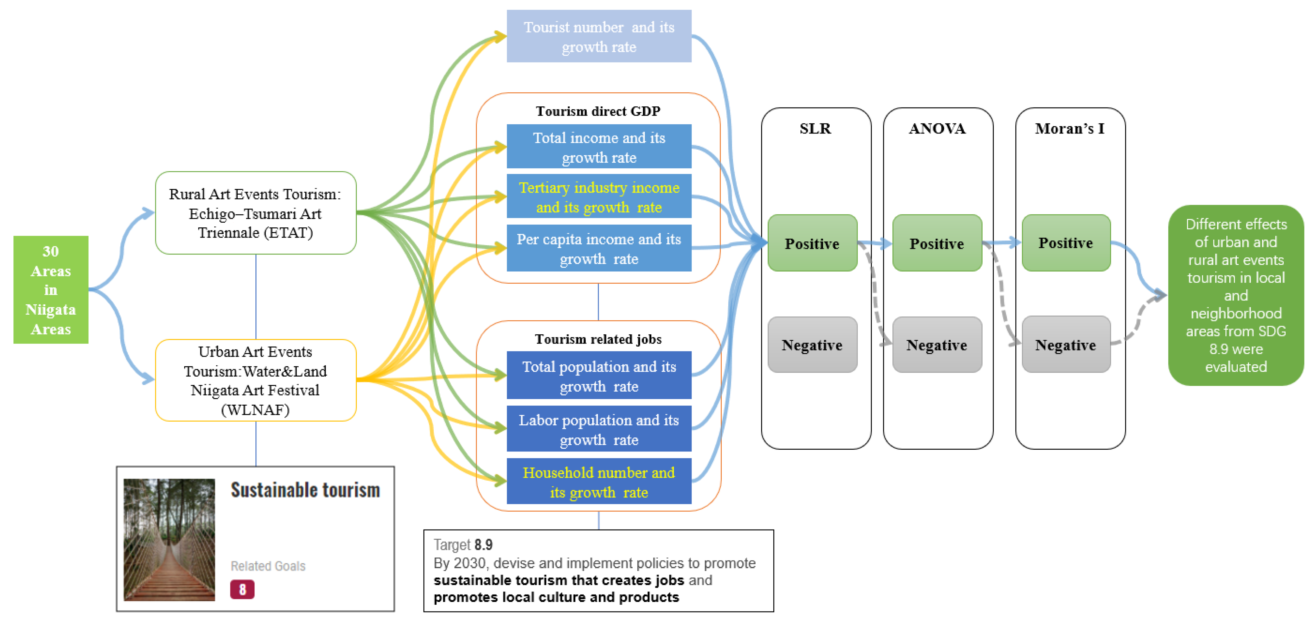
:1. Introduction
2. Literature Review
2.1. Sustainable Development Goals (SDGs) and Sustainable Tourism
2.2. Urban and Rural Arts Event Tourism
2.3. Art Event Tourism and Economics: Total Income, Tertiary industry Income, and Per capita Income
2.4. Art Event Tourism and Population: Total Population, Labor Population, and Household Number
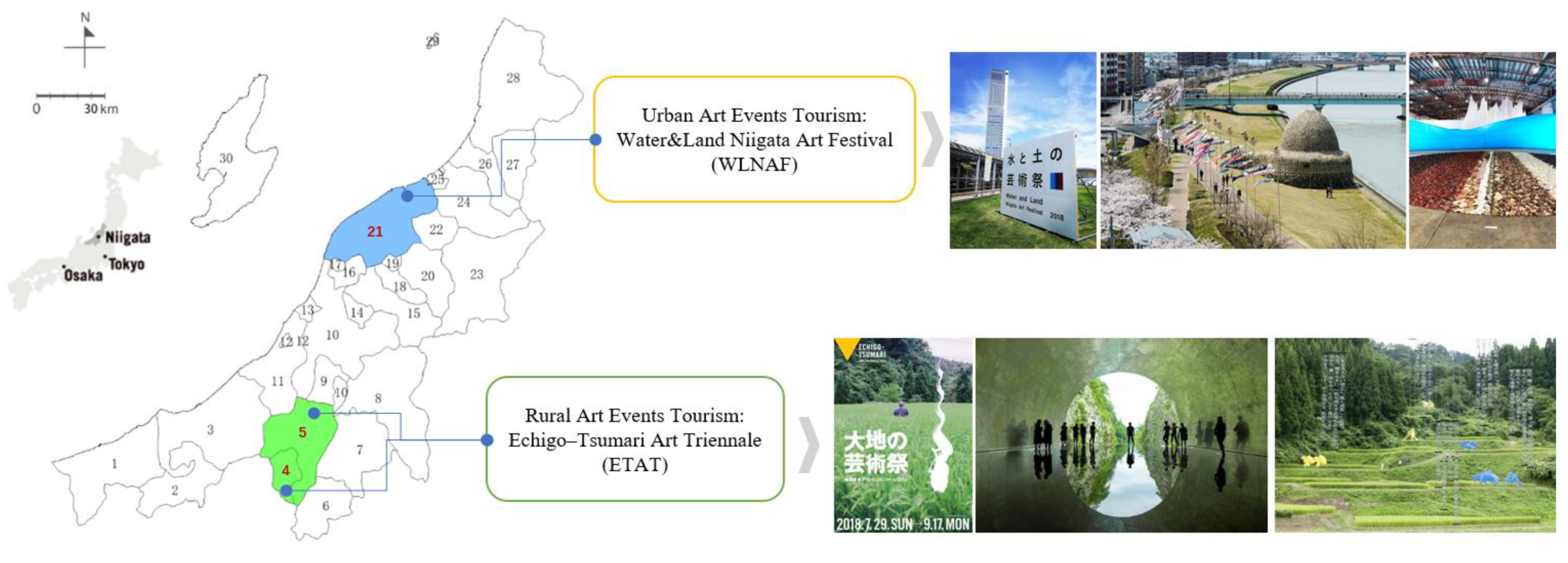
3. Exhibition-Driven Tourism in Niigata
3.1. Japanese Arts Events: Festival and Exhibition
3.2. Urban and Rural Arts Events: ETAT and WLNAF in Niigata
4. Methods
4.1. Panel Data
4.2. The Descriptive Statistics
4.3. Simple Linear Regression (SLR)
4.4. The One-Way ANOVA Analysis
4.5. Moran’s I
5. Results
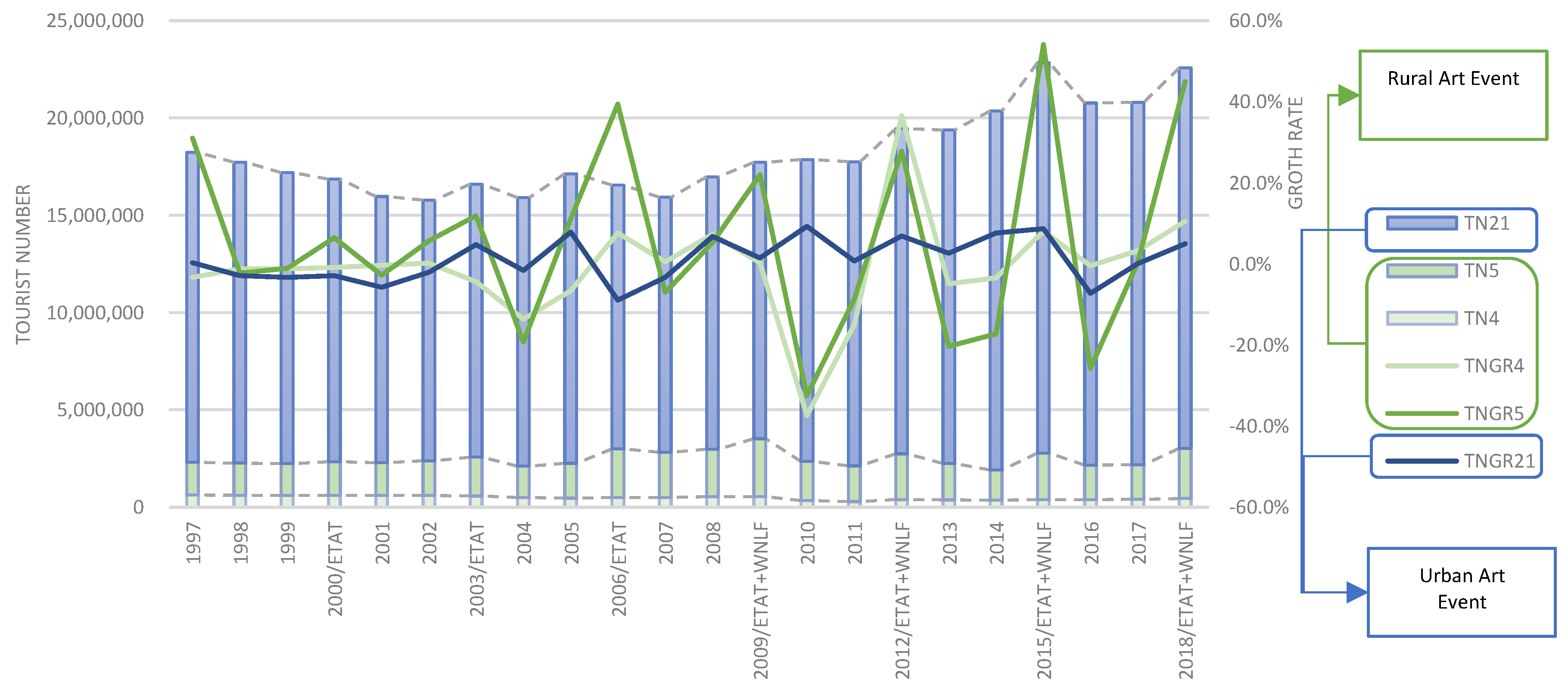
5.1. The Descriptive Statistics
5.2. Simple Linear Regression (SLR) between Hosting Areas and Niigata Areas
5.3. One-Way ANOVA: Total Income
5.3.1. Total Income
5.3.2. Tertiary Industry Income
5.3.3. Per Capita Income
5.4. One-Way ANOVA: Population
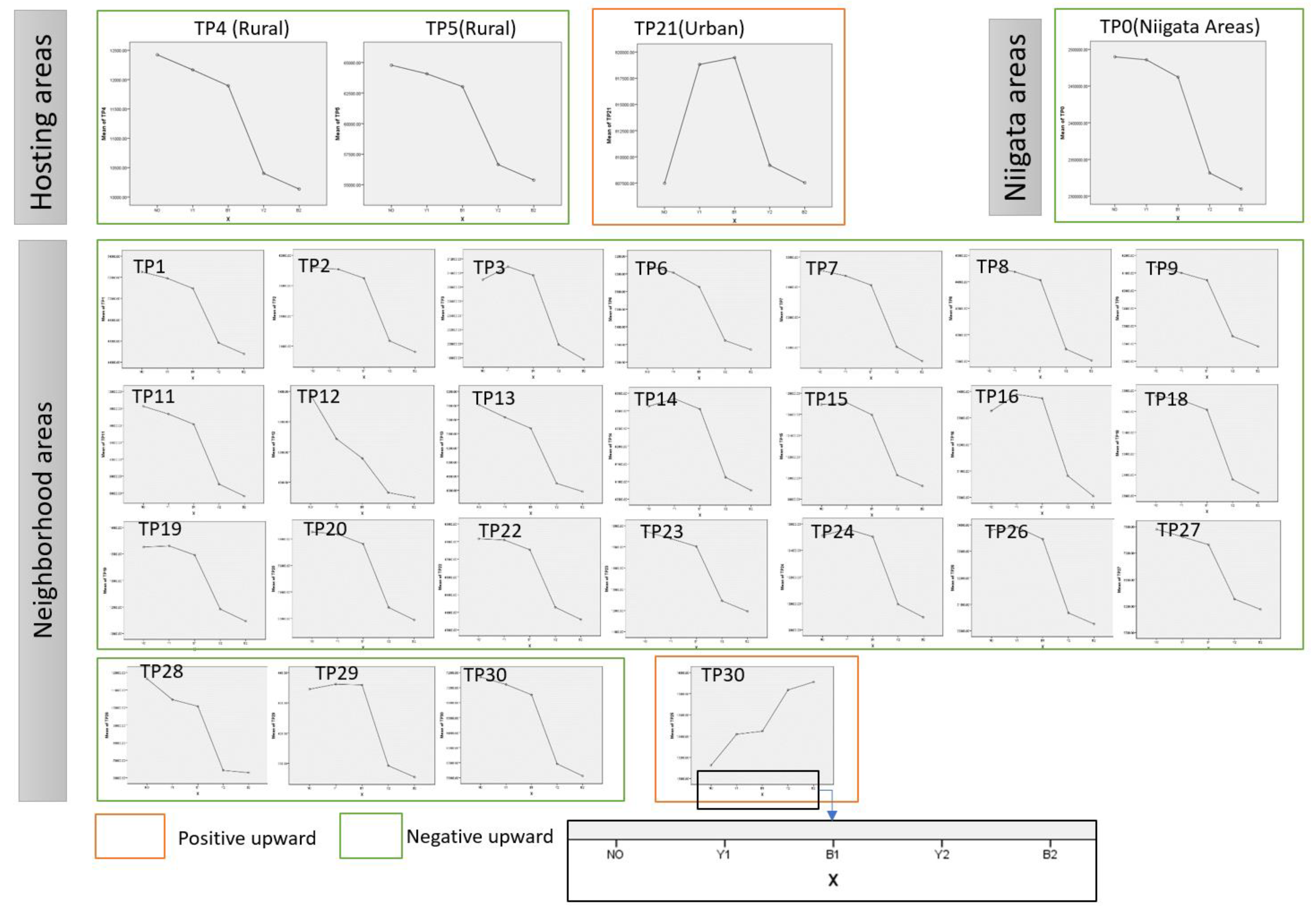
5.4.1. Total Population
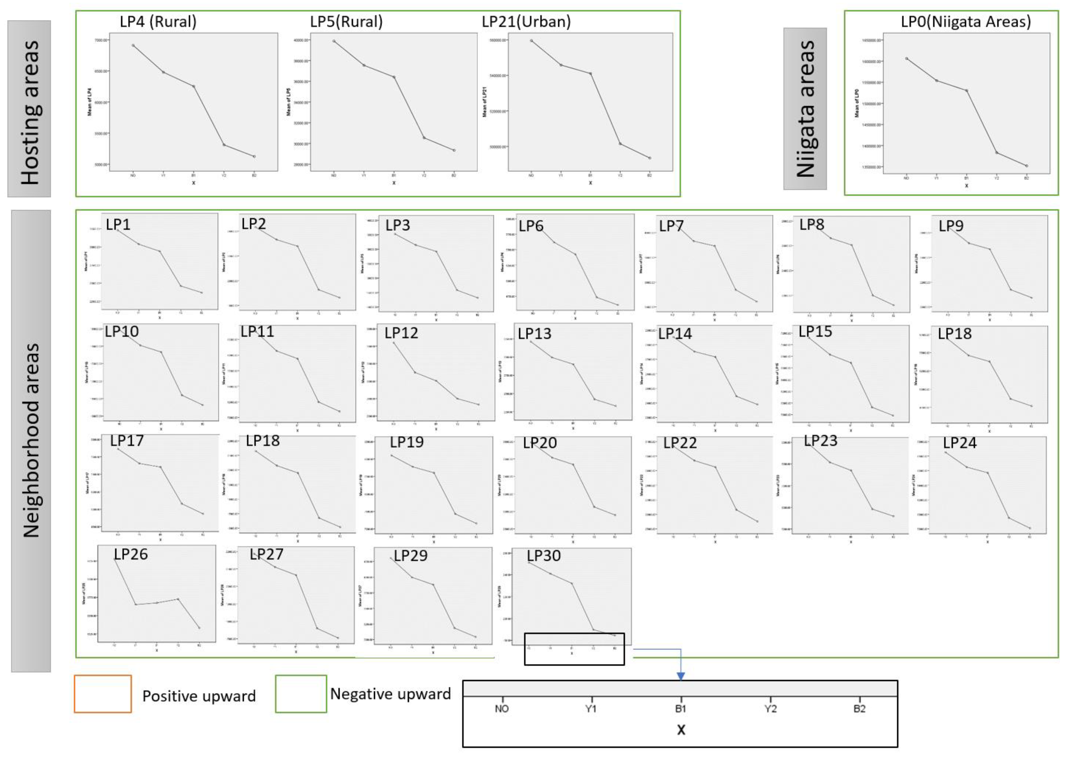
5.4.2. Labor Population
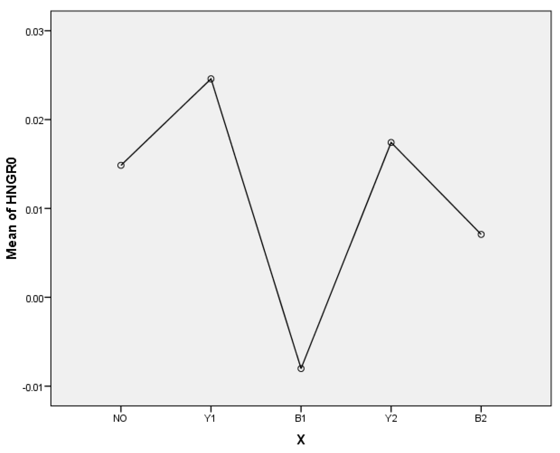
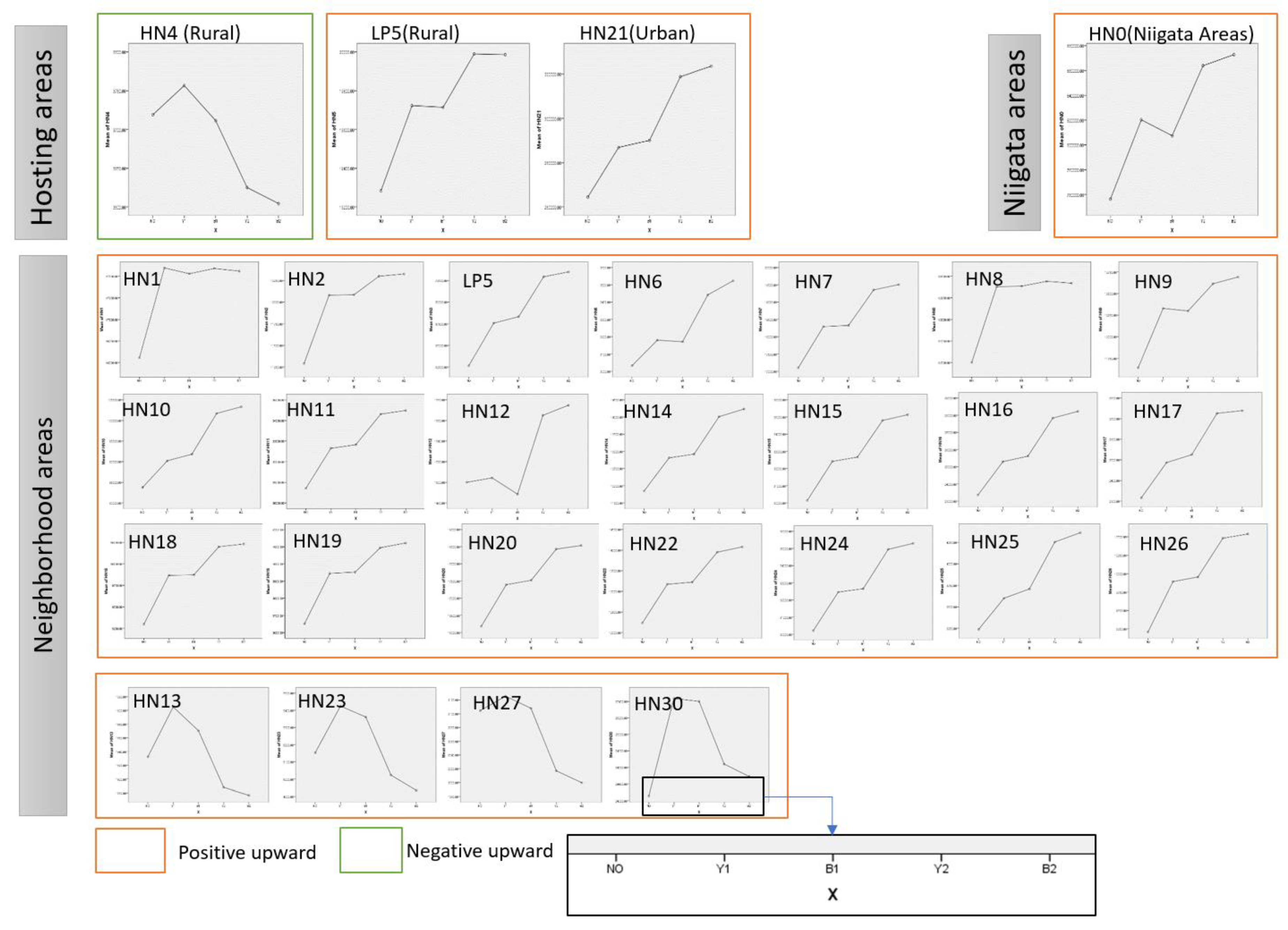
5.4.3. Household Number
5.5. Spatial Impact
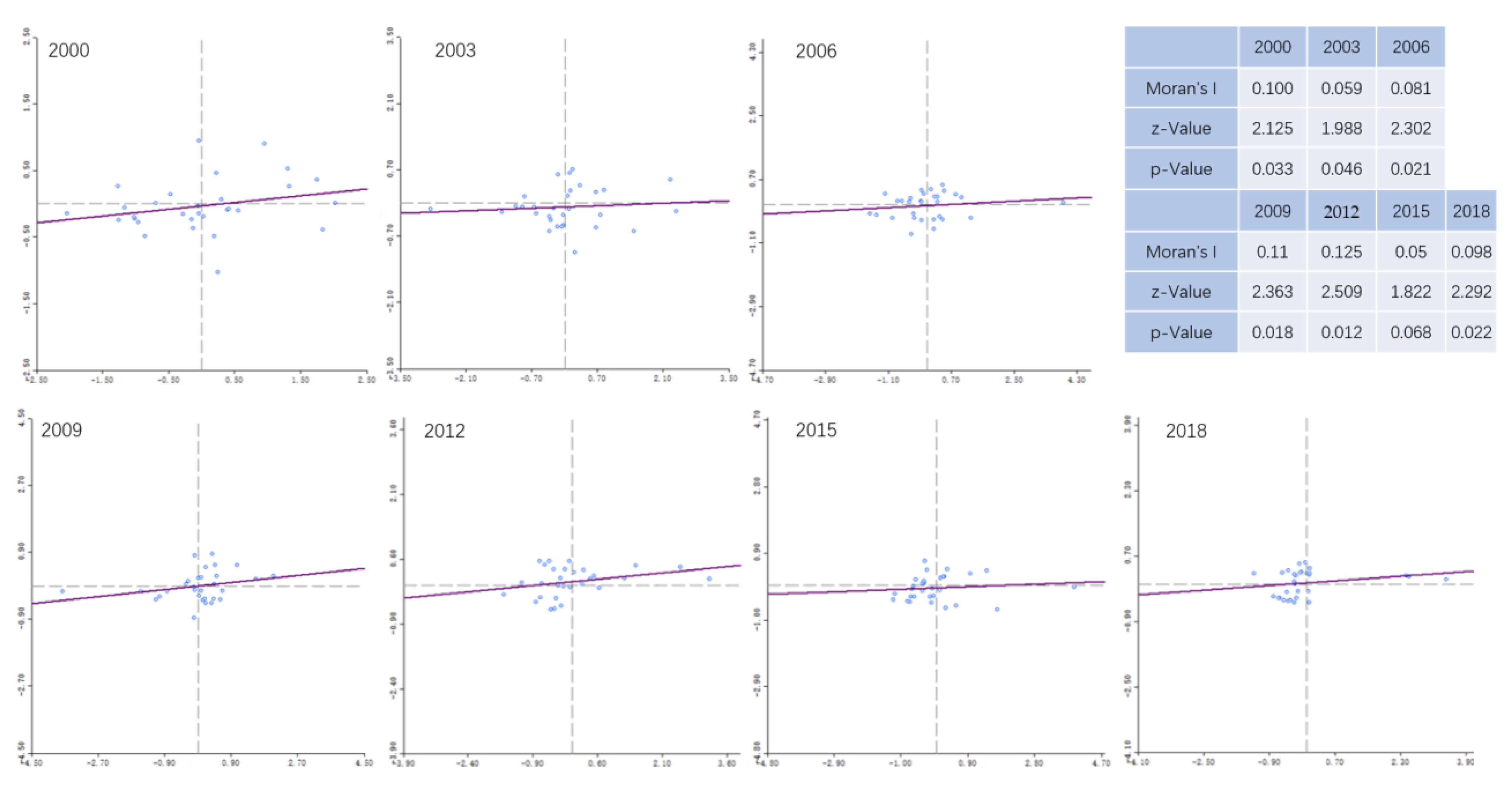
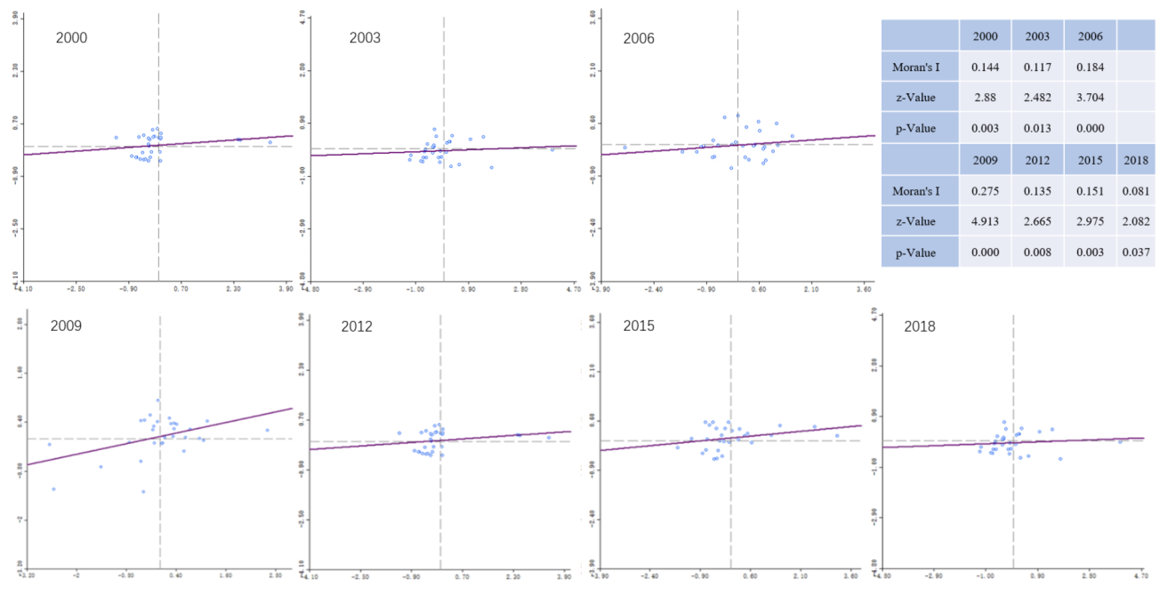
5.5.1. Moran’s I Test of Tourism Indicators
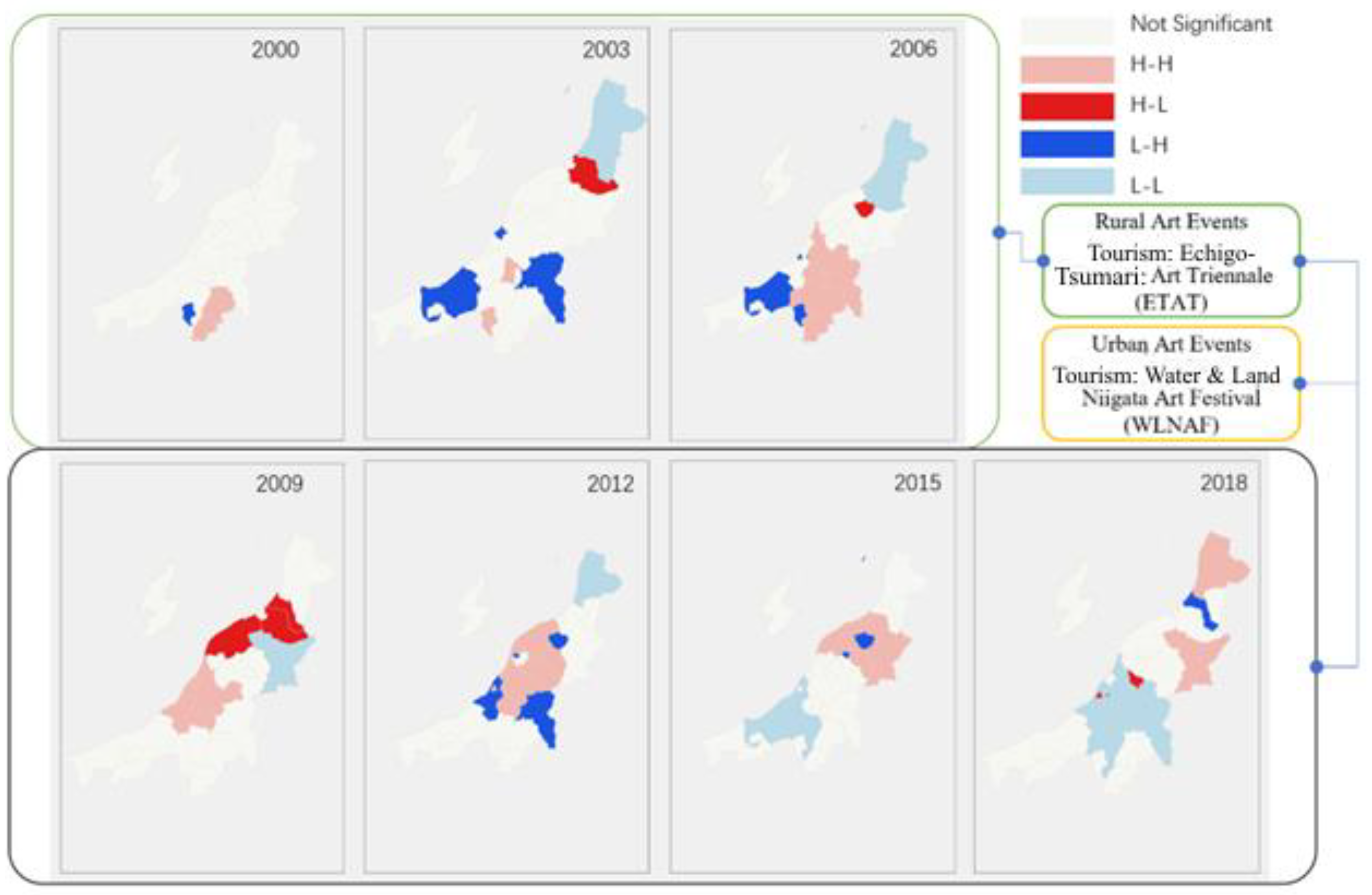
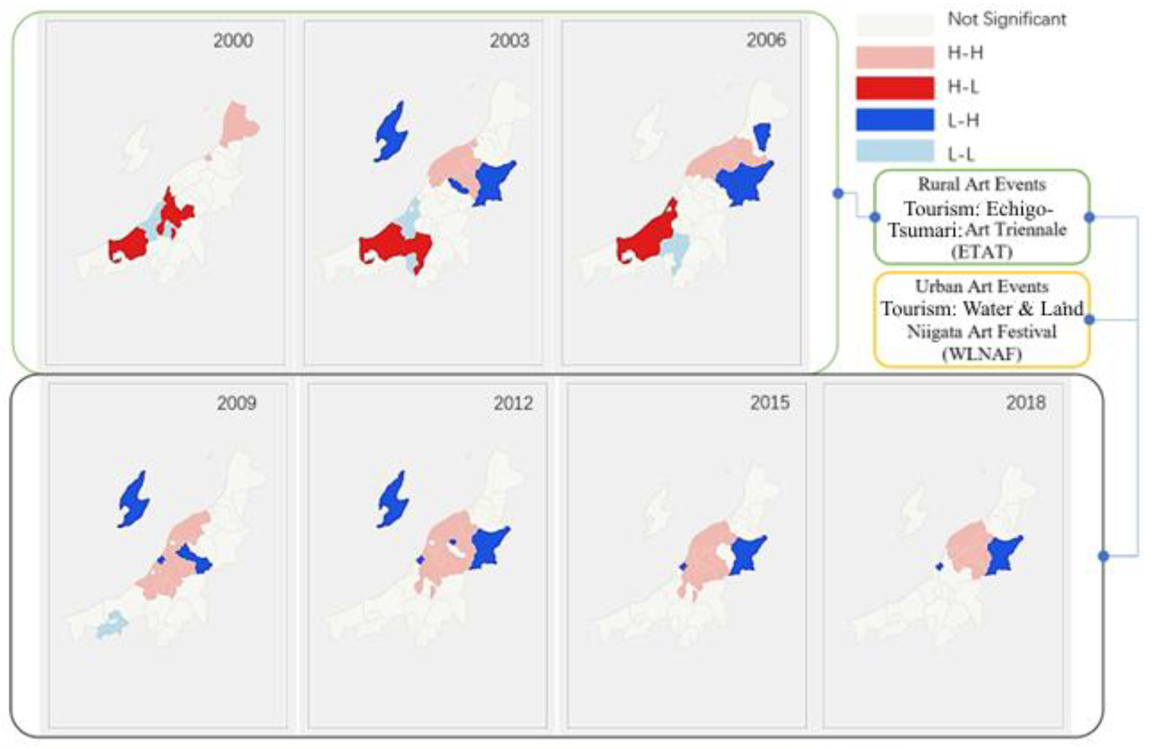
5.5.2. Local Indicators of Spatial Association (LISA)
- Tertiary Industry Income
- Household Number
6. Discussion and Conclusions
6.1. Implications for Theory
6.2. Implications for Practitioners and Policy Makers
6.3. Limitations and Future Research Directions
Author Contributions
Funding
Data Availability Statement
Conflicts of Interest
Appendix A

| I | J | MD (I–J) | Sig. | MD (I–J) | Sig. | MD (I–J) | Sig. | MD (I–J) | Sig. | MD (I–J) | Sig. | MD (I–J) | Sig. | ||||||
|---|---|---|---|---|---|---|---|---|---|---|---|---|---|---|---|---|---|---|---|
| NO | Y1 | TI0 | 368,697 | 0.035 | TI5 | 8963 | 0.156 | TI9 | 4579 | 0.524 | TI15 | 8638 | 0.439 | TI19 | 1265 | 0.257 | TI28 | −27,532 | 0.432 |
| B1 | 499,675 | 0.003 | 16,832 | 0.006 | 18,499 | 0.009 | 18,076 | 0.075 | 1700 | 0.088 | −26,258 | 0.388 | |||||||
| Y2 | 1,032,318 | 0.000 | 33,075 | 0.000 | 55,381 | 0.000 | 29,131 | 0.018 | 4487 | 0.001 | −88,540 | 0.021 | |||||||
| B2 | 1,037,094 | 0.000 | 32,726 | 0.000 | 57,300 | 0.000 | 32,666 | 0.006 | 4651 | 0.000 | −87,016 | 0.016 | |||||||
| Y1 | B1 | 130,979 | 0.355 | 7869 | 0.151 | 13,920 | 0.038 | 9437 | 0.332 | 434 | 0.647 | 1273 | 0.966 | ||||||
| Y2 | 663,621 | 0.001 | 24,112 | 0.001 | 50,802 | 0.000 | 20,493 | 0.080 | 3222 | 0.009 | −61,009 | 0.095 | |||||||
| B2 | 668,398 | 0.000 | 23,763 | 0.001 | 52,720 | 0.000 | 24,028 | 0.033 | 3385 | 0.004 | −59,484 | 0.083 | |||||||
| B1 | Y2 | 532,643 | 0.002 | 16,244 | 0.007 | 36,882 | 0.000 | 11,056 | 0.259 | 2787 | 0.009 | −62,282 | 0.053 | ||||||
| B2 | 537,419 | 0.001 | 15,895 | 0.005 | 38,801 | 0.000 | 14,591 | 0.111 | 2951 | 0.004 | −60,758 | 0.040 | |||||||
| Y2 | B2 | 4777 | 0.975 | −349 | 0.951 | 1919 | 0.774 | 3535 | 0.733 | 164 | 0.873 | 1524 | 0.962 | ||||||
| NO | Y1 | TI1 | 31,152 | 0.007 | TI6 | 20,488 | 0.043 | TI11 | 87,731 | 0.047 | TI16 | 9601 | 0.256 | TI20 | 11,730 | 0.025 | TI29 | 649 | 0.190 |
| B1 | 38,015 | 0.001 | 24,254 | 0.009 | 98,712 | 0.013 | 15,898 | 0.040 | 17,046 | 0.001 | 620 | 0.151 | |||||||
| Y2 | 52,347 | 0.000 | 40,538 | 0.001 | 222,228 | 0.000 | 42,672 | 0.000 | 10,628 | 0.039 | 1663 | 0.003 | |||||||
| B2 | 41,769 | 0.001 | 41,363 | 0.000 | 214,491 | 0.000 | 44,040 | 0.000 | 16,286 | 0.002 | 1649 | 0.002 | |||||||
| Y1 | B1 | 6863 | 0.438 | 3766 | 0.644 | 10,981 | 0.758 | 6297 | 0.385 | 5317 | 0.209 | −30 | 0.943 | ||||||
| Y2 | 21,196 | 0.051 | 20,049 | 0.047 | 134,497 | 0.005 | 33,070 | 0.001 | −1102 | 0.817 | 1014 | 0.049 | |||||||
| B2 | 10,618 | 0.272 | 20,874 | 0.029 | 126,761 | 0.005 | 34,438 | 0.000 | 4556 | 0.314 | 1000 | 0.040 | |||||||
| B1 | Y2 | 14,333 | 0.118 | 16,283 | 0.060 | 123,516 | 0.003 | 26,773 | 0.002 | −6418 | 0.134 | 1044 | 0.023 | ||||||
| B2 | 3755 | 0.640 | 17,108 | 0.034 | 115,779 | 0.003 | 28,141 | 0.001 | −761 | 0.840 | 1029 | 0.015 | |||||||
| Y2 | B2 | −10,578 | 0.274 | 825 | 0.925 | −7737 | 0.840 | 1368 | 0.859 | 5658 | 0.216 | −14 | 0.975 | ||||||
| NO | Y1 | TI2 | −3636 | 0.850 | TI7 | 17,011 | 0.072 | TI12 | 21,189 | 0.069 | TI17 | −2321 | 0.075 | TI23 | 15,027 | 0.002 | TI30 | 28,740 | 0.071 |
| B1 | −613 | 0.971 | 19,581 | 0.021 | 23,113 | 0.026 | −70 | 0.948 | 16,305 | 0.000 | 42,350 | 0.005 | |||||||
| Y2 | 76,648 | 0.001 | 30,317 | 0.004 | 49,754 | 0.000 | 4488 | 0.002 | 24,038 | 0.000 | 84,034 | 0.000 | |||||||
| B2 | 90,940 | 0.000 | 26,580 | 0.006 | 46,569 | 0.000 | 4031 | 0.003 | 25,775 | 0.000 | 83,113 | 0.000 | |||||||
| Y1 | B1 | 3023 | 0.856 | 2570 | 0.739 | 1924 | 0.839 | 2251 | 0.049 | 1278 | 0.717 | 13,610 | 0.304 | ||||||
| Y2 | 80,284 | 0.001 | 13,307 | 0.150 | 28,565 | 0.019 | 6809 | 0.000 | 9011 | 0.040 | 55,295 | 0.002 | |||||||
| B2 | 94,576 | 0.000 | 9569 | 0.261 | 25,380 | 0.024 | 6352 | 0.000 | 10,747 | 0.012 | 54,373 | 0.001 | |||||||
| B1 | Y2 | 77,261 | 0.000 | 10,736 | 0.178 | 26,641 | 0.013 | 4558 | 0.001 | 7733 | 0.042 | 41,685 | 0.006 | ||||||
| B2 | 91,553 | 0.000 | 6999 | 0.328 | 23,456 | 0.015 | 4101 | 0.001 | 9469 | 0.009 | 40,763 | 0.004 | |||||||
| Y2 | B2 | 14,292 | 0.433 | −3738 | 0.654 | −3185 | 0.756 | −456 | 0.692 | 1736 | 0.649 | −922 | 0.948 | ||||||
| NO | Y1 | TI4 | 6930 | 0.018 | TI8 | 22,350 | 0.012 | TI13 | 2633 | 0.006 | TI18 | 8694 | 0.018 | TI27 | 2704 | 0.177 | |||
| B1 | 8792 | 0.002 | 29,952 | 0.001 | 2152 | 0.008 | 13,969 | 0.000 | 4016 | 0.029 | |||||||||
| Y2 | 13,769 | 0.000 | 50,716 | 0.000 | 5494 | 0.000 | 18,667 | 0.000 | 7425 | 0.002 | |||||||||
| B2 | 13,477 | 0.000 | 52,020 | 0.000 | 4926 | 0.000 | 19,577 | 0.000 | 7899 | 0.001 | |||||||||
| Y1 | B1 | 1862 | 0.421 | 7601 | 0.274 | −481 | 0.502 | 5275 | 0.081 | 1311 | 0.439 | ||||||||
| Y2 | 6839 | 0.019 | 28,366 | 0.002 | 2861 | 0.003 | 9974 | 0.008 | 4721 | 0.026 | |||||||||
| B2 | 6546 | 0.017 | 29,670 | 0.001 | 2293 | 0.009 | 10,884 | 0.003 | 5195 | 0.011 | |||||||||
| B1 | Y2 | 4977 | 0.044 | 20,764 | 0.008 | 3342 | 0.000 | 4699 | 0.116 | 3410 | 0.057 | ||||||||
| B2 | 4684 | 0.038 | 22,069 | 0.003 | 2774 | 0.001 | 5609 | 0.046 | 3883 | 0.022 | |||||||||
| Y2 | B2 | −292 | 0.906 | 1304 | 0.859 | −567 | 0.464 | 910 | 0.768 | 474 | 0.794 |
| I | J | MD (I–J) | Sig. | MD (I–J) | Sig. | MD (I–J) | Sig. | MD (I–J) | Sig. | MD (I–J) | Sig. | MD (I–J) | Sig. | ||||||
|---|---|---|---|---|---|---|---|---|---|---|---|---|---|---|---|---|---|---|---|
| NO | Y1 | TII0 | −1,387,250 | 0.000 | TII4 | −12,260 | 0.003 | TII9 | −26,337 | 0.000 | TII15 | −60,416 | 0.000 | TII19 | −5622 | 0.000 | TII23 | −12,459 | 0.000 |
| B1 | −1,473,547 | 0.000 | −10,549 | 0.004 | −22,391 | 0.000 | −59,950 | 0.000 | −5404 | 0.000 | −9798 | 0.000 | |||||||
| Y2 | −1,104,793 | 0.000 | −8083 | 0.043 | −15,628 | 0.000 | −53,109 | 0.000 | −4254 | 0.000 | −2905 | 0.196 | |||||||
| B2 | −1,102,233 | 0.000 | −8520 | 0.034 | −15,805 | 0.000 | −58,273 | 0.000 | −4737 | 0.000 | −4146 | 0.076 | |||||||
| Y1 | B1 | −86297 | 0.394 | 1711 | 0.589 | 3946 | 0.026 | 466 | 0.915 | 218 | 0.513 | 2661 | 0.180 | ||||||
| Y2 | 282,457 | 0.035 | 4177 | 0.281 | 10,709 | 0.000 | 7307 | 0.179 | 1368 | 0.005 | 9554 | 0.001 | |||||||
| B2 | 285,017 | 0.033 | 3740 | 0.332 | 10,532 | 0.000 | 2143 | 0.681 | 885 | 0.044 | 8313 | 0.004 | |||||||
| B1 | Y2 | 368,754 | 0.007 | 2466 | 0.495 | 6763 | 0.003 | 6841 | 0.184 | 1150 | 0.010 | 6893 | 0.008 | ||||||
| B2 | 371,314 | 0.007 | 2030 | 0.573 | 6586 | 0.003 | 1677 | 0.734 | 667 | 0.097 | 5652 | 0.022 | |||||||
| Y2 | B2 | 2560 | 0.984 | −437 | 0.916 | −178 | 0.930 | −5164 | 0.373 | −483 | 0.279 | −1241 | 0.619 | ||||||
| NO | Y1 | TII1 | −31,655 | 0.000 | TII6 | −24,428 | 0.001 | TII10 | −198,932 | 0.000 | TII16 | −51,674 | 0.000 | TII20 | −25,494 | 0.000 | TII24 | −52,867 | 0.000 |
| B1 | −29,380 | 0.000 | −16,389 | 0.007 | −216,664 | 0.000 | −51,694 | 0.000 | −25,021 | 0.000 | −53,023 | 0.000 | |||||||
| Y2 | −15,695 | 0.002 | −5919 | 0.343 | −186,900 | 0.000 | −39,084 | 0.000 | −17,284 | 0.000 | −43,875 | 0.000 | |||||||
| B2 | −13,776 | 0.004 | −9879 | 0.128 | −198,395 | 0.000 | −44,050 | 0.000 | −16,726 | 0.000 | −51,922 | 0.000 | |||||||
| Y1 | B1 | 2275 | 0.501 | 8039 | 0.156 | −17,732 | 0.094 | −20 | 0.991 | 473 | 0.823 | −156 | 0.932 | ||||||
| Y2 | 15,961 | 0.002 | 18,509 | 0.014 | 12,032 | 0.318 | 12,590 | 0.000 | 8210 | 0.008 | 8992 | 0.002 | |||||||
| B2 | 17,879 | 0.001 | 14,549 | 0.043 | 537 | 0.963 | 7624 | 0.005 | 8768 | 0.005 | 945 | 0.665 | |||||||
| B1 | Y2 | 13,686 | 0.004 | 10,470 | 0.109 | 29,764 | 0.021 | 12,610 | 0.000 | 7737 | 0.008 | 9149 | 0.001 | ||||||
| B2 | 15,604 | 0.002 | 6510 | 0.299 | 18,269 | 0.123 | 7645 | 0.003 | 8295 | 0.005 | 1101 | 0.596 | |||||||
| Y2 | B2 | 1919 | 0.663 | −3960 | 0.577 | −11,495 | 0.381 | −4966 | 0.057 | 558 | 0.840 | −8048 | 0.006 | ||||||
| NO | Y1 | TII2 | −23,899 | 0.000 | TII7 | −48,607 | 0.000 | TII13 | −2579 | 0.000 | TII17 | −5170 | 0.000 | TII21 | −360,834 | 0.007 | TII25 | −57,498 | 0.000 |
| B1 | −21,321 | 0.000 | −49,990 | 0.000 | −2074 | 0.000 | −4697 | 0.000 | −577,842 | 0.000 | −31,931 | 0.001 | |||||||
| Y2 | −6733 | 0.008 | −38,916 | 0.000 | −1380 | 0.006 | −2411 | 0.000 | −482,311 | 0.003 | −41,433 | 0.001 | |||||||
| B2 | −8345 | 0.002 | −39,750 | 0.000 | −1145 | 0.016 | −3056 | 0.000 | −489,660 | 0.003 | −31,937 | 0.004 | |||||||
| Y1 | B1 | 2578 | 0.185 | −1382 | 0.608 | 506 | 0.179 | 473 | 0.143 | −217,009 | 0.072 | 25,566 | 0.008 | ||||||
| Y2 | 17,165 | 0.000 | 9692 | 0.011 | 1199 | 0.017 | 2759 | 0.000 | −121,478 | 0.369 | 16,065 | 0.110 | |||||||
| B2 | 15,554 | 0.000 | 8857 | 0.018 | 1435 | 0.006 | 2114 | 0.000 | −128,827 | 0.342 | 25,561 | 0.019 | |||||||
| B1 | Y2 | 14,588 | 0.000 | 11,074 | 0.004 | 694 | 0.111 | 2286 | 0.000 | 95,531 | 0.453 | −9501 | 0.300 | ||||||
| B2 | 12,976 | 0.000 | 10,240 | 0.006 | 929 | 0.041 | 1641 | 0.001 | 88,182 | 0.488 | −5 | 1.000 | |||||||
| Y2 | B2 | −1612 | 0.512 | −835 | 0.812 | 236 | 0.618 | −645 | 0.129 | −7349 | 0.960 | 9496 | 0.367 | ||||||
| NO | Y1 | TII3 | −114,203 | 0.000 | TII8 | −30,797 | 0.000 | TII14 | −21,259 | 0.000 | TII18 | −15,040 | 0.000 | TII22 | −19,366 | 0.000 | TII26 | −14,246 | 0.000 |
| B1 | −112,225 | 0.000 | −31,882 | 0.000 | −24,050 | 0.000 | −14,735 | 0.000 | −19,525 | 0.000 | −12,136 | 0.000 | |||||||
| Y2 | −115,113 | 0.000 | −18,074 | 0.000 | −24,652 | 0.000 | −9703 | 0.000 | −15,332 | 0.000 | −10,555 | 0.000 | |||||||
| B2 | −141,230 | 0.000 | −17,005 | 0.000 | −23,850 | 0.000 | −8402 | 0.000 | −15,353 | 0.000 | −10,116 | 0.000 | |||||||
| Y1 | B1 | 1978 | 0.850 | −1085 | 0.644 | −2792 | 0.050 | 305 | 0.796 | −159 | 0.904 | 2110 | 0.171 | ||||||
| Y2 | −910 | 0.942 | 12,723 | 0.001 | −3394 | 0.047 | 5336 | 0.003 | 4034 | 0.025 | 3691 | 0.056 | |||||||
| B2 | −27,027 | 0.051 | 13,792 | 0.000 | −2592 | 0.115 | 6637 | 0.001 | 4013 | 0.026 | 4131 | 0.036 | |||||||
| B1 | Y2 | −2888 | 0.808 | 13,809 | 0.000 | −602 | 0.681 | 5032 | 0.003 | 4193 | 0.016 | 1581 | 0.353 | ||||||
| B2 | −29,005 | 0.031 | 14,877 | 0.000 | 200 | 0.891 | 6333 | 0.001 | 4172 | 0.017 | 2020 | 0.241 | |||||||
| Y2 | B2 | −26,117 | 0.079 | 1069 | 0.728 | 802 | 0.636 | 1301 | 0.406 | −21 | 0.990 | 440 | 0.819 |
| I | J | MD (I–J) | Sig. | MD (I–J) | Sig. | MD (I–J) | Sig. | MD (I–J) | Sig. | MD (I–J) | Sig. | MD (I–J) | Sig. | ||||||
|---|---|---|---|---|---|---|---|---|---|---|---|---|---|---|---|---|---|---|---|
| NO | Y1 | PCI0 | 128 | 0.078 | PCI4 | 202.333 | 0.065 | PCI9 | 38 | 0.628 | PCI17 | 148 | 0.119 | PCI24 | 155 | 0.033 | PCI29 | 338.3 | 0.125 |
| B1 | 165 | 0.011 | 281.5 | 0.005 | 154 | 0.029 | 154 | 0.060 | 193 | 0.003 | 561.4 | 0.006 | |||||||
| Y2 | 228 | 0.004 | 399.667 | 0.001 | 296 | 0.001 | 365 | 0.001 | 299 | 0.000 | 721.3 | 0.003 | |||||||
| B2 | 176 | 0.009 | 378.6 | 0.001 | 244 | 0.002 | 315 | 0.001 | 259 | 0.000 | 654.7 | 0.003 | |||||||
| Y1 | B1 | 37 | 0.564 | 79.167 | 0.414 | 116 | 0.119 | 6 | 0.947 | 38 | 0.549 | 223.2 | 0.266 | ||||||
| Y2 | 100 | 0.188 | 197.333 | 0.089 | 259 | 0.006 | 216 | 0.039 | 144 | 0.059 | 383.0 | 0.106 | |||||||
| B2 | 48 | 0.469 | 176.267 | 0.09 | 206 | 0.012 | 167 | 0.070 | 104 | 0.120 | 316.4 | 0.133 | |||||||
| B1 | Y2 | 63 | 0.334 | 118.167 | 0.229 | 142 | 0.061 | 211 | 0.023 | 107 | 0.102 | 159.8 | 0.421 | ||||||
| B2 | 11 | 0.840 | 97.1 | 0.248 | 90 | 0.156 | 162 | 0.038 | 67 | 0.223 | 93.2 | 0.581 | |||||||
| Y2 | B2 | −52 | 0.438 | −21.067 | 0.832 | −53 | 0.481 | −49 | 0.576 | −40 | 0.536 | −66.6 | 0.743 | ||||||
| NO | Y1 | PCI1 | 192 | 0.044 | PCI5 | 176.333 | 0.02 | PCI11 | −1 | 0.994 | PCI19 | 109 | 0.047 | PCI25 | 194 | 0.225 | PCI30 | 295.3 | 0.017 |
| B1 | 206 | 0.014 | 226.667 | 0.001 | 38 | 0.587 | 147 | 0.004 | 229 | 0.098 | 393.8 | 0.001 | |||||||
| Y2 | 303 | 0.003 | 324 | 0 | 203 | 0.022 | 268 | 0.000 | 494 | 0.006 | 621.7 | 0.000 | |||||||
| B2 | 286 | 0.002 | 307 | 0 | 173 | 0.026 | 255 | 0.000 | 441 | 0.005 | 602.2 | 0.000 | |||||||
| Y1 | B1 | 14 | 0.864 | 50.333 | 0.436 | 38 | 0.614 | 37 | 0.438 | 35 | 0.812 | 98.5 | 0.350 | ||||||
| Y2 | 110 | 0.259 | 147.667 | 0.06 | 203 | 0.031 | 159 | 0.010 | 299 | 0.088 | 326.3 | 0.014 | |||||||
| B2 | 94 | 0.282 | 130.667 | 0.062 | 174 | 0.038 | 146 | 0.008 | 246 | 0.114 | 306.9 | 0.010 | |||||||
| B1 | Y2 | 96 | 0.256 | 97.333 | 0.142 | 165 | 0.041 | 122 | 0.020 | 265 | 0.082 | 227.8 | 0.041 | ||||||
| B2 | 80 | 0.271 | 80.333 | 0.156 | 136 | 0.049 | 108 | 0.016 | 212 | 0.102 | 208.4 | 0.030 | |||||||
| Y2 | B2 | −17 | 0.847 | −17 | 0.797 | −30 | 0.705 | −13 | 0.785 | −53 | 0.723 | −19.5 | 0.856 | ||||||
| NO | Y1 | PCI2 | 192 | 0.101 | PCI7 | 124.167 | 0.043 | PCI12 | −192 | 0.158 | PCI21 | 142 | 0.041 | PCI27 | 222 | 0.027 | |||
| B1 | 245 | 0.018 | 162.833 | 0.004 | −53 | 0.638 | 173 | 0.005 | 262 | 0.004 | |||||||||
| Y2 | 537 | 0.000 | 214.167 | 0.002 | 187 | 0.168 | 206 | 0.005 | 379 | 0.001 | |||||||||
| B2 | 504 | 0.000 | 181.9 | 0.002 | 249 | 0.044 | 159 | 0.012 | 314 | 0.001 | |||||||||
| Y1 | B1 | 53 | 0.609 | 38.667 | 0.471 | 139 | 0.262 | 32 | 0.597 | 40 | 0.644 | ||||||||
| Y2 | 346 | 0.010 | 90 | 0.156 | 379 | 0.015 | 64 | 0.359 | 157 | 0.128 | |||||||||
| B2 | 312 | 0.009 | 57.733 | 0.302 | 440 | 0.003 | 18 | 0.776 | 92 | 0.311 | |||||||||
| B1 | Y2 | 292 | 0.011 | 51.333 | 0.342 | 240 | 0.063 | 33 | 0.589 | 117 | 0.187 | ||||||||
| B2 | 259 | 0.009 | 19.067 | 0.677 | 301 | 0.010 | −14 | 0.782 | 52 | 0.487 | |||||||||
| Y2 | B2 | −33 | 0.756 | −32.267 | 0.559 | 61 | 0.627 | −47 | 0.454 | −65 | 0.466 | ||||||||
| NO | Y1 | PCI3 | 82 | 0.336 | PCI8 | 221.167 | 0.01 | PCI13 | 181 | 0.01 | PCI23 | 347 | 0.001 | PCI28 | 292 | 0.005 | |||
| B1 | 171 | 0.026 | 274.5 | 0.001 | 184 | 0.003 | 400 | 0.000 | 346 | 0.000 | |||||||||
| Y2 | 294 | 0.003 | 365.167 | 0 | 208 | 0.004 | 542 | 0.000 | 488 | 0.000 | |||||||||
| B2 | 185 | 0.021 | 318.3 | 0 | 143 | 0.018 | 519 | 0.000 | 447 | 0.000 | |||||||||
| Y1 | B1 | 89 | 0.261 | 53.333 | 0.461 | 3 | 0.961 | 54 | 0.517 | 55 | 0.519 | ||||||||
| Y2 | 212 | 0.029 | 144 | 0.096 | 27 | 0.685 | 195 | 0.053 | 197 | 0.056 | |||||||||
| B2 | 104 | 0.209 | 97.133 | 0.201 | −38 | 0.526 | 172 | 0.055 | 155 | 0.088 | |||||||||
| B1 | Y2 | 123 | 0.128 | 90.667 | 0.217 | 25 | 0.674 | 142 | 0.099 | 142 | 0.105 | ||||||||
| B2 | 14 | 0.829 | 43.8 | 0.479 | −41 | 0.414 | 119 | 0.105 | 101 | 0.174 | |||||||||
| Y2 | B2 | −108 | 0.189 | −46.867 | 0.529 | −66 | 0.283 | −23 | 0.790 | −41 | 0.634 |
| I | J | MD (I–J) | Sig. | MD (I–J) | Sig. | MD (I–J) | Sig. | MD (I–J) | Sig. | MD (I–J) | Sig. | MD (I–J) | Sig. | ||||||
|---|---|---|---|---|---|---|---|---|---|---|---|---|---|---|---|---|---|---|---|
| NO | Y1 | TP0 | 4060 | 0.926 | TP5 | 708 | 0.733 | TP11 | 915 | 0.702 | TP16 | −625 | 0.573 | TP22 | 68 | 0.949 | TP27 | 142 | 0.648 |
| B1 | 27,691 | 0.469 | 1758 | 0.333 | 2125 | 0.310 | −478 | 0.618 | 620 | 0.505 | 290 | 0.286 | |||||||
| Y2 | 158,290 | 0.001 | 8122 | 0.000 | 9175 | 0.001 | 2448 | 0.027 | 3878 | 0.001 | 1316 | 0.000 | |||||||
| B2 | 180,083 | 0.000 | 9392 | 0.000 | 10,587 | 0.000 | 3214 | 0.002 | 4569 | 0.000 | 1511 | 0.000 | |||||||
| Y1 | B1 | 23,631 | 0.536 | 1050 | 0.560 | 1210 | 0.560 | 147 | 0.878 | 552 | 0.552 | 149 | 0.580 | ||||||
| Y2 | 154,230 | 0.001 | 7414 | 0.001 | 8261 | 0.001 | 3073 | 0.007 | 3810 | 0.001 | 1174 | 0.001 | |||||||
| B2 | 176,023 | 0.000 | 8684 | 0.000 | 9672 | 0.000 | 3839 | 0.000 | 4501 | 0.000 | 1369 | 0.000 | |||||||
| B1 | Y2 | 130,599 | 0.001 | 6364 | 0.001 | 7050 | 0.001 | 2926 | 0.003 | 3258 | 0.001 | 1025 | 0.000 | ||||||
| B2 | 152,392 | 0.000 | 7634 | 0.000 | 8462 | 0.000 | 3692 | 0.000 | 3949 | 0.000 | 1220 | 0.000 | |||||||
| Y2 | B2 | 21,794 | 0.510 | 1270 | 0.418 | 1412 | 0.434 | 766 | 0.361 | 691 | 0.392 | 195 | 0.405 | ||||||
| NO | Y1 | TP1 | 614 | 0.709 | TP6 | 78 | 0.654 | TP12 | 290 | 0.045 | TP18 | 198 | 0.847 | TP23 | 341 | 0.666 | TP28 | 11,893 | 0.324 |
| B1 | 1565 | 0.279 | 239 | 0.123 | 419 | 0.002 | 664 | 0.459 | 712 | 0.304 | 15,663 | 0.140 | |||||||
| Y2 | 6693 | 0.000 | 847 | 0.000 | 645 | 0.000 | 3973 | 0.000 | 3275 | 0.000 | 52,188 | 0.000 | |||||||
| B2 | 7734 | 0.000 | 949 | 0.000 | 677 | 0.000 | 4599 | 0.000 | 3773 | 0.000 | 53,492 | 0.000 | |||||||
| Y1 | B1 | 951 | 0.507 | 161 | 0.290 | 129 | 0.283 | 466 | 0.602 | 371 | 0.589 | 3769 | 0.715 | ||||||
| Y2 | 6079 | 0.001 | 769 | 0.000 | 355 | 0.011 | 3775 | 0.001 | 2934 | 0.001 | 40,295 | 0.002 | |||||||
| B2 | 7120 | 0.000 | 871 | 0.000 | 387 | 0.003 | 4401 | 0.000 | 3431 | 0.000 | 41,598 | 0.000 | |||||||
| B1 | Y2 | 5128 | 0.001 | 607 | 0.000 | 226 | 0.047 | 3310 | 0.001 | 2563 | 0.001 | 36,526 | 0.001 | ||||||
| B2 | 6169 | 0.000 | 710 | 0.000 | 258 | 0.009 | 3936 | 0.000 | 3061 | 0.000 | 37,829 | 0.000 | |||||||
| Y2 | B2 | 1041 | 0.403 | 103 | 0.434 | 32 | 0.757 | 626 | 0.421 | 498 | 0.404 | 1303 | 0.884 | ||||||
| NO | Y1 | TP2 | 131 | 0.911 | TP7 | 371 | 0.798 | TP13 | 175 | 0.444 | TP19 | −21 | 0.949 | TP24 | −477 | 0.762 | TP29 | −3 | 0.831 |
| B1 | 719 | 0.483 | 992 | 0.433 | 331 | 0.104 | 152 | 0.596 | 90 | 0.947 | −3 | 0.834 | |||||||
| Y2 | 4856 | 0.000 | 5091 | 0.001 | 1110 | 0.000 | 1171 | 0.001 | 5192 | 0.002 | 51 | 0.002 | |||||||
| B2 | 5588 | 0.000 | 6042 | 0.000 | 1225 | 0.000 | 1400 | 0.000 | 6171 | 0.000 | 58 | 0.000 | |||||||
| Y1 | B1 | 588 | 0.566 | 621 | 0.622 | 156 | 0.431 | 173 | 0.547 | 568 | 0.678 | 1 | 0.971 | ||||||
| Y2 | 4725 | 0.000 | 4721 | 0.002 | 935 | 0.000 | 1192 | 0.001 | 5670 | 0.001 | 54 | 0.001 | |||||||
| B2 | 5456 | 0.000 | 5671 | 0.000 | 1050 | 0.000 | 1421 | 0.000 | 6648 | 0.000 | 61 | 0.000 | |||||||
| B1 | Y2 | 4137 | 0.000 | 4100 | 0.002 | 779 | 0.000 | 1019 | 0.001 | 5102 | 0.001 | 53 | 0.000 | ||||||
| B2 | 4868 | 0.000 | 5050 | 0.000 | 894 | 0.000 | 1248 | 0.000 | 6081 | 0.000 | 61 | 0.000 | |||||||
| Y2 | B2 | 731 | 0.411 | 951 | 0.386 | 115 | 0.504 | 229 | 0.359 | 979 | 0.412 | 8 | 0.524 | ||||||
| NO | Y1 | TP3 | −1840 | 0.577 | TP8 | 408 | 0.796 | TP14 | −211 | 0.722 | TP20 | 167 | 0.915 | TP25 | −294 | 0.013 | TP30 | 982 | 0.710 |
| B1 | −605 | 0.832 | 1031 | 0.454 | 84 | 0.871 | 906 | 0.508 | −322 | 0.003 | 2364 | 0.308 | |||||||
| Y2 | 9189 | 0.007 | 6235 | 0.000 | 2011 | 0.002 | 5700 | 0.001 | −712 | 0.000 | 11,543 | 0.000 | |||||||
| B2 | 11,274 | 0.000 | 7087 | 0.000 | 2382 | 0.000 | 6638 | 0.000 | −788 | 0.000 | 13,140 | 0.000 | |||||||
| Y1 | B1 | 1235 | 0.665 | 624 | 0.649 | 295 | 0.568 | 738 | 0.589 | −28 | 0.769 | 1382 | 0.547 | ||||||
| Y2 | 11,029 | 0.002 | 5827 | 0.001 | 2222 | 0.001 | 5533 | 0.001 | −417 | 0.001 | 10,561 | 0.000 | |||||||
| B2 | 13,114 | 0.000 | 6680 | 0.000 | 2593 | 0.000 | 6470 | 0.000 | −493 | 0.000 | 12,158 | 0.000 | |||||||
| B1 | Y2 | 9793 | 0.001 | 5204 | 0.000 | 1927 | 0.001 | 4795 | 0.001 | −390 | 0.000 | 9178 | 0.000 | ||||||
| B2 | 11,879 | 0.000 | 6056 | 0.000 | 2298 | 0.000 | 5732 | 0.000 | −466 | 0.000 | 10,775 | 0.000 | |||||||
| Y2 | B2 | 2085 | 0.401 | 852 | 0.474 | 371 | 0.409 | 937 | 0.430 | −76 | 0.357 | 1597 | 0.424 | ||||||
| NO | Y1 | TP4 | 257 | 0.570 | TP9 | 355 | 0.739 | TP15 | −176 | 0.917 | TP21 | −11337 | 0.013 | TP26 | −106 | 0.885 | |||
| B1 | 528 | 0.187 | 764 | 0.410 | 966 | 0.511 | −11991 | 0.003 | 348 | 0.585 | |||||||||
| Y2 | 2021 | 0.000 | 3936 | 0.001 | 6657 | 0.000 | −1714 | 0.662 | 3131 | 0.000 | |||||||||
| B2 | 2288 | 0.000 | 4510 | 0.000 | 7682 | 0.000 | −46 | 0.989 | 3548 | 0.000 | |||||||||
| Y1 | B1 | 270 | 0.492 | 410 | 0.657 | 1142 | 0.438 | −653 | 0.857 | 454 | 0.477 | ||||||||
| Y2 | 1763 | 0.000 | 3582 | 0.002 | 6833 | 0.000 | 9623 | 0.022 | 3237 | 0.000 | |||||||||
| B2 | 2030 | 0.000 | 4155 | 0.000 | 7858 | 0.000 | 11,291 | 0.004 | 3654 | 0.000 | |||||||||
| B1 | Y2 | 1493 | 0.000 | 3172 | 0.001 | 5691 | 0.000 | 10,276 | 0.005 | 2783 | 0.000 | ||||||||
| B2 | 1760 | 0.000 | 3746 | 0.000 | 6716 | 0.000 | 11,944 | 0.000 | 3200 | 0.000 | |||||||||
| Y2 | B2 | 267 | 0.434 | 574 | 0.474 | 1025 | 0.421 | 1668 | 0.596 | 417 | 0.451 |
| I | J | MD (I–J) | Sig. | MD (I–J) | Sig. | MD (I–J) | Sig. | MD (I–J) | Sig. | MD (I–J) | Sig. | MD (I–J) | Sig. | ||||||
|---|---|---|---|---|---|---|---|---|---|---|---|---|---|---|---|---|---|---|---|
| NO | Y1 | LP0 | 52,509 | 0.318 | LP5 | 2342 | 0.242 | LP10 | 4385 | 0.418 | LP15 | 2894 | 0.223 | LP20 | 1747 | 0.307 | LP26 | 761 | 0.389 |
| B1 | 76,059 | 0.102 | 3474 | 0.052 | 6289 | 0.186 | 4298 | 0.044 | 2533 | 0.095 | 1221 | 0.118 | |||||||
| Y2 | 223,150 | 0.000 | 9341 | 0.000 | 18,643 | 0.001 | 11,930 | 0.000 | 7391 | 0.000 | 4269 | 0.000 | |||||||
| B2 | 254,377 | 0.000 | 10,547 | 0.000 | 21,445 | 0.000 | 13,342 | 0.000 | 8332 | 0.000 | 4819 | 0.000 | |||||||
| Y1 | B1 | 23,550 | 0.601 | 1133 | 0.508 | 1904 | 0.682 | 1404 | 0.489 | 787 | 0.592 | 460 | 0.545 | ||||||
| Y2 | 170,641 | 0.002 | 7000 | 0.001 | 14,258 | 0.010 | 9036 | 0.000 | 5645 | 0.002 | 3508 | 0.000 | |||||||
| B2 | 201,867 | 0.000 | 8206 | 0.000 | 17,061 | 0.001 | 10,448 | 0.000 | 6585 | 0.000 | 4059 | 0.000 | |||||||
| B1 | Y2 | 147,091 | 0.002 | 5867 | 0.001 | 12,354 | 0.008 | 7632 | 0.000 | 4858 | 0.002 | 3049 | 0.000 | ||||||
| B2 | 178,317 | 0.000 | 7073 | 0.000 | 15,156 | 0.000 | 9044 | 0.000 | 5798 | 0.000 | 3599 | 0.000 | |||||||
| Y2 | B2 | 31,227 | 0.426 | 1206 | 0.417 | 2803 | 0.489 | 1411 | 0.423 | 940 | 0.461 | 550 | 0.405 | ||||||
| NO | Y1 | LP1 | 1927 | 0.226 | LP6 | 337 | 0.129 | LP11 | 3131 | 0.237 | LP16 | 2283 | 0.191 | LP21 | 13,764 | 0.315 | LP27 | 307 | 0.214 |
| B1 | 2903 | 0.042 | 531 | 0.009 | 4376 | 0.064 | 3129 | 0.045 | 18,539 | 0.125 | 426 | 0.054 | |||||||
| Y2 | 7711 | 0.000 | 1225 | 0.000 | 11,322 | 0.000 | 8254 | 0.000 | 58,084 | 0.000 | 1121 | 0.000 | |||||||
| B2 | 8622 | 0.000 | 1349 | 0.000 | 12,838 | 0.000 | 9241 | 0.000 | 66,103 | 0.000 | 1264 | 0.000 | |||||||
| Y1 | B1 | 975 | 0.473 | 194 | 0.304 | 1244 | 0.582 | 846 | 0.568 | 4775 | 0.684 | 118 | 0.575 | ||||||
| Y2 | 5783 | 0.001 | 888 | 0.000 | 8191 | 0.003 | 5972 | 0.001 | 44,319 | 0.002 | 814 | 0.002 | |||||||
| B2 | 6695 | 0.000 | 1012 | 0.000 | 9706 | 0.000 | 6958 | 0.000 | 52,339 | 0.000 | 957 | 0.000 | |||||||
| B1 | Y2 | 4808 | 0.001 | 694 | 0.001 | 6947 | 0.003 | 5126 | 0.001 | 39,544 | 0.001 | 695 | 0.002 | ||||||
| B2 | 5719 | 0.000 | 817 | 0.000 | 8462 | 0.000 | 6112 | 0.000 | 47,564 | 0.000 | 838 | 0.000 | |||||||
| Y2 | B2 | 911 | 0.440 | 124 | 0.447 | 1515 | 0.441 | 986 | 0.444 | 8020 | 0.432 | 143 | 0.436 | ||||||
| NO | Y1 | LP2 | 1011 | 0.367 | LP7 | 1554 | 0.306 | LP12 | 341 | 0.015 | LP17 | 166 | 0.476 | LP22 | 989 | 0.416 | LP29 | 10 | 0.376 |
| B1 | 1541 | 0.121 | 1945 | 0.145 | 438 | 0.001 | 208 | 0.306 | 1434 | 0.180 | 19 | 0.067 | |||||||
| Y2 | 5049 | 0.000 | 5479 | 0.001 | 642 | 0.000 | 627 | 0.008 | 4371 | 0.001 | 62 | 0.000 | |||||||
| B2 | 5692 | 0.000 | 6433 | 0.000 | 710 | 0.000 | 743 | 0.001 | 5169 | 0.000 | 67 | 0.000 | |||||||
| Y1 | B1 | 530 | 0.583 | 391 | 0.763 | 97 | 0.391 | 42 | 0.835 | 445 | 0.671 | 9 | 0.382 | ||||||
| Y2 | 4038 | 0.001 | 3924 | 0.011 | 301 | 0.021 | 461 | 0.044 | 3382 | 0.007 | 51 | 0.000 | |||||||
| B2 | 4681 | 0.000 | 4879 | 0.001 | 368 | 0.002 | 577 | 0.007 | 4180 | 0.000 | 57 | 0.000 | |||||||
| B1 | Y2 | 3508 | 0.001 | 3533 | 0.007 | 204 | 0.057 | 420 | 0.031 | 2938 | 0.006 | 42 | 0.000 | ||||||
| B2 | 4151 | 0.000 | 4488 | 0.000 | 272 | 0.004 | 535 | 0.002 | 3735 | 0.000 | 48 | 0.000 | |||||||
| Y2 | B2 | 643 | 0.443 | 955 | 0.400 | 68 | 0.488 | 116 | 0.507 | 798 | 0.383 | 5 | 0.537 | ||||||
| NO | Y1 | LP3 | 3823 | 0.368 | LP8 | 1346 | 0.324 | LP13 | 218 | 0.208 | LP18 | 1005 | 0.316 | LP23 | 856 | 0.149 | LP30 | 2097 | 0.296 |
| B1 | 6057 | 0.108 | 1894 | 0.117 | 311 | 0.045 | 1504 | 0.091 | 1229 | 0.022 | 3341 | 0.063 | |||||||
| Y2 | 19,427 | 0.000 | 5958 | 0.000 | 792 | 0.000 | 4599 | 0.000 | 3014 | 0.000 | 10,141 | 0.000 | |||||||
| B2 | 22,076 | 0.000 | 6752 | 0.000 | 885 | 0.000 | 5225 | 0.000 | 3342 | 0.000 | 11,335 | 0.000 | |||||||
| Y1 | B1 | 2234 | 0.542 | 547 | 0.640 | 93 | 0.529 | 499 | 0.561 | 374 | 0.458 | 1244 | 0.470 | ||||||
| Y2 | 15,604 | 0.001 | 4611 | 0.001 | 574 | 0.002 | 3594 | 0.001 | 2158 | 0.001 | 8045 | 0.000 | |||||||
| B2 | 18,253 | 0.000 | 5405 | 0.000 | 667 | 0.000 | 4220 | 0.000 | 2486 | 0.000 | 9238 | 0.000 | |||||||
| B1 | Y2 | 13,370 | 0.001 | 4064 | 0.001 | 481 | 0.002 | 3095 | 0.001 | 1784 | 0.001 | 6801 | 0.000 | ||||||
| B2 | 16,019 | 0.000 | 4858 | 0.000 | 574 | 0.000 | 3721 | 0.000 | 2113 | 0.000 | 7994 | 0.000 | |||||||
| Y2 | B2 | 2649 | 0.405 | 794 | 0.436 | 93 | 0.466 | 626 | 0.403 | 328 | 0.451 | 1194 | 0.424 | ||||||
| NO | Y1 | LP4 | 433 | 0.197 | LP9 | 1329 | 0.247 | LP14 | 996 | 0.277 | LP19 | 325 | 0.451 | LP24 | 2030 | 0.370 | |||
| B1 | 660 | 0.030 | 1807 | 0.077 | 1368 | 0.092 | 497 | 0.191 | 2816 | 0.158 | |||||||||
| Y2 | 1601 | 0.000 | 5080 | 0.000 | 4070 | 0.000 | 1674 | 0.000 | 9014 | 0.000 | |||||||||
| B2 | 1788 | 0.000 | 5723 | 0.000 | 4632 | 0.000 | 1947 | 0.000 | 10,435 | 0.000 | |||||||||
| Y1 | B1 | 227 | 0.428 | 478 | 0.626 | 372 | 0.635 | 172 | 0.644 | 786 | 0.686 | ||||||||
| Y2 | 1168 | 0.001 | 3751 | 0.002 | 3074 | 0.002 | 1349 | 0.003 | 6984 | 0.003 | |||||||||
| B2 | 1355 | 0.000 | 4394 | 0.000 | 3636 | 0.000 | 1622 | 0.000 | 8405 | 0.000 | |||||||||
| B1 | Y2 | 942 | 0.002 | 3273 | 0.001 | 2702 | 0.001 | 1177 | 0.002 | 6197 | 0.002 | ||||||||
| B2 | 1128 | 0.000 | 3916 | 0.000 | 3264 | 0.000 | 1450 | 0.000 | 7618 | 0.000 | |||||||||
| Y2 | B2 | 187 | 0.451 | 642 | 0.451 | 562 | 0.411 | 273 | 0.399 | 1421 | 0.402 |
| I | J | MD (I−J) | Sig. | MD (I−J) | Sig. | MD (I−J) | Sig. | MD (I−J) | Sig. | MD (I−J) | Sig. | MD (I−J) | Sig. | ||||||
|---|---|---|---|---|---|---|---|---|---|---|---|---|---|---|---|---|---|---|---|
| NO | Y1 | HN0 | −63,893 | 0.002 | HN5 | −440 | 0.014 | HN10 | −6453 | 0.045 | HN15 | −2271 | 0.007 | HN20 | −1211 | 0.001 | HN25 | −363 | 0.101 |
| B1 | −51,060 | 0.004 | −431 | 0.008 | −8073 | 0.008 | −2527 | 0.001 | −1339 | 0.000 | −471 | 0.022 | |||||||
| Y2 | −107,511 | 0.000 | −707 | 0.000 | −17,946 | 0.000 | −4657 | 0.000 | −2246 | 0.000 | −1017 | 0.000 | |||||||
| B2 | −116,484 | 0.000 | −703 | 0.000 | −19,571 | 0.000 | −4993 | 0.000 | −2351 | 0.000 | −1125 | 0.000 | |||||||
| Y1 | B1 | 12,834 | 0.351 | 9 | 0.943 | −1620 | 0.495 | −255 | 0.664 | −128 | 0.601 | −109 | 0.512 | ||||||
| Y2 | −43,618 | 0.007 | −267 | 0.066 | −11,492 | 0.000 | −2386 | 0.001 | −1035 | 0.001 | −655 | 0.002 | |||||||
| B2 | −52,591 | 0.001 | −263 | 0.043 | −13,117 | 0.000 | −2722 | 0.000 | −1140 | 0.000 | −763 | 0.000 | |||||||
| B1 | Y2 | −56,452 | 0.000 | −276 | 0.028 | −9873 | 0.000 | −2131 | 0.001 | −907 | 0.001 | −546 | 0.002 | ||||||
| B2 | −65,424 | 0.000 | −272 | 0.011 | −11,498 | 0.000 | −2467 | 0.000 | −1012 | 0.000 | −654 | 0.000 | |||||||
| Y2 | B2 | −8973 | 0.449 | 4 | 0.972 | −1625 | 0.430 | −336 | 0.510 | −105 | 0.621 | −108 | 0.451 | ||||||
| NO | Y1 | HN1 | −1039 | 0.000 | HN6 | −147 | 0.340 | HN11 | −1943 | 0.001 | HN16 | −1941 | 0.022 | HN21 | −22,450 | 0.038 | HN26 | −684 | 0.002 |
| B1 | −972 | 0.000 | −138 | 0.317 | −2118 | 0.000 | −2261 | 0.004 | −25,634 | 0.011 | −748 | 0.000 | |||||||
| Y2 | −1033 | 0.000 | −409 | 0.010 | −3603 | 0.000 | −4479 | 0.000 | −54,355 | 0.000 | −1274 | 0.000 | |||||||
| B2 | −1002 | 0.000 | −491 | 0.001 | −3779 | 0.000 | −4871 | 0.000 | −59,178 | 0.000 | −1332 | 0.000 | |||||||
| Y1 | B1 | 66 | 0.536 | 9 | 0.939 | −175 | 0.663 | −320 | 0.599 | −3184 | 0.687 | −64 | 0.670 | ||||||
| Y2 | 6 | 0.957 | −262 | 0.052 | −1661 | 0.001 | −2538 | 0.001 | −31,906 | 0.001 | −590 | 0.002 | |||||||
| B2 | 37 | 0.720 | −343 | 0.006 | −1836 | 0.000 | −2930 | 0.000 | −36,728 | 0.000 | −648 | 0.000 | |||||||
| B1 | Y2 | −60 | 0.539 | −271 | 0.020 | −1486 | 0.001 | −2218 | 0.001 | −28,722 | 0.001 | −527 | 0.001 | ||||||
| B2 | −30 | 0.716 | −352 | 0.001 | −1661 | 0.000 | −2610 | 0.000 | −33,544 | 0.000 | −584 | 0.000 | |||||||
| Y2 | B2 | 31 | 0.742 | −82 | 0.429 | −175 | 0.615 | −392 | 0.460 | −4823 | 0.483 | −58 | 0.656 | ||||||
| NO | Y1 | HN2 | −790 | 0.000 | HN7 | −1190 | 0.007 | HN12 | −4 | 0.822 | HN17 | −171 | 0.001 | HN22 | −939 | 0.003 | HN27 | −21 | 0.580 |
| B1 | −795 | 0.000 | −1223 | 0.002 | 12 | 0.508 | −210 | 0.000 | −991 | 0.001 | −4 | 0.918 | |||||||
| Y2 | −1009 | 0.000 | −2250 | 0.000 | −65 | 0.002 | −410 | 0.000 | −1717 | 0.000 | 88 | 0.024 | |||||||
| B2 | −1035 | 0.000 | −2405 | 0.000 | −75 | 0.000 | −423 | 0.000 | −1846 | 0.000 | 105 | 0.005 | |||||||
| Y1 | B1 | −5 | 0.961 | −33 | 0.913 | 16 | 0.297 | −39 | 0.283 | −52 | 0.810 | 18 | 0.551 | ||||||
| Y2 | −219 | 0.067 | −1061 | 0.004 | −61 | 0.001 | −239 | 0.000 | −778 | 0.003 | 109 | 0.003 | |||||||
| B2 | −245 | 0.024 | −1215 | 0.001 | −70 | 0.000 | −252 | 0.000 | −906 | 0.000 | 126 | 0.000 | |||||||
| B1 | Y2 | −214 | 0.037 | −1027 | 0.001 | −77 | 0.000 | −201 | 0.000 | −727 | 0.001 | 91 | 0.003 | ||||||
| B2 | −240 | 0.007 | −1182 | 0.000 | −86 | 0.000 | −214 | 0.000 | −855 | 0.000 | 108 | 0.000 | |||||||
| Y2 | B2 | −26 | 0.773 | −155 | 0.559 | −10 | 0.455 | −13 | 0.668 | −128 | 0.491 | 17 | 0.502 | ||||||
| NO | Y1 | HN3 | −4934 | 0.004 | HN8 | −877 | 0.000 | HN13 | −73 | 0.028 | HN18 | −570 | 0.000 | HN23 | −271 | 0.089 | HN30 | −1179 | 0.002 |
| B1 | −5679 | 0.000 | −883 | 0.000 | −38 | 0.179 | −574 | 0.000 | −207 | 0.142 | −1143 | 0.001 | |||||||
| Y2 | −10,292 | 0.000 | −939 | 0.000 | 45 | 0.140 | −902 | 0.000 | 131 | 0.371 | −383 | 0.224 | |||||||
| B2 | −10,863 | 0.000 | −918 | 0.000 | 56 | 0.048 | −934 | 0.000 | 219 | 0.110 | −232 | 0.414 | |||||||
| Y1 | B1 | −745 | 0.530 | −6 | 0.957 | 35 | 0.160 | −5 | 0.960 | 64 | 0.591 | 36 | 0.887 | ||||||
| Y2 | −5358 | 0.000 | −62 | 0.611 | 117 | 0.000 | −332 | 0.004 | 402 | 0.005 | 796 | 0.008 | |||||||
| B2 | −5929 | 0.000 | −41 | 0.704 | 128 | 0.000 | −365 | 0.001 | 490 | 0.000 | 947 | 0.001 | |||||||
| B1 | Y2 | −4613 | 0.000 | −56 | 0.586 | 83 | 0.001 | −327 | 0.001 | 338 | 0.005 | 761 | 0.004 | ||||||
| B2 | −5184 | 0.000 | −35 | 0.685 | 94 | 0.000 | −360 | 0.000 | 426 | 0.000 | 911 | 0.000 | |||||||
| Y2 | B2 | −571 | 0.577 | 21 | 0.828 | 11 | 0.588 | −33 | 0.685 | 88 | 0.396 | 151 | 0.492 | ||||||
| NO | Y1 | HN4 | −38 | 0.386 | HN9 | −687 | 0.000 | HN14 | −962 | 0.023 | HN19 | −293 | 0.000 | HN24 | −2245 | 0.013 | |||
| B1 | 8 | 0.842 | −657 | 0.000 | −1071 | 0.006 | −300 | 0.000 | −2442 | 0.004 | |||||||||
| Y2 | 94 | 0.031 | −972 | 0.000 | −2160 | 0.000 | −442 | 0.000 | −4730 | 0.000 | |||||||||
| B2 | 115 | 0.006 | −1049 | 0.000 | −2384 | 0.000 | −469 | 0.000 | −5083 | 0.000 | |||||||||
| Y1 | B1 | 45 | 0.184 | 30 | 0.777 | −108 | 0.722 | −7 | 0.886 | −198 | 0.759 | ||||||||
| Y2 | 132 | 0.002 | −285 | 0.019 | −1198 | 0.002 | −149 | 0.014 | −2486 | 0.002 | |||||||||
| B2 | 152 | 0.000 | −363 | 0.002 | −1421 | 0.000 | −177 | 0.002 | −2839 | 0.000 | |||||||||
| B1 | Y2 | 86 | 0.010 | −315 | 0.004 | −1090 | 0.001 | −142 | 0.006 | −2288 | 0.001 | ||||||||
| B2 | 107 | 0.000 | −392 | 0.000 | −1313 | 0.000 | −169 | 0.000 | −2641 | 0.000 | |||||||||
| Y2 | B2 | 21 | 0.477 | −78 | 0.393 | −224 | 0.401 | −27 | 0.539 | −353 | 0.529 |
References
- Takahashi, N. The Role of Arts Festivals in Contemporary Japan; De Montfort University: Leicester, UK, 2015; ISBN 9781857214260. [Google Scholar]
- Fletcher, R. Five Capitals for Festivals: Integrated Reporting of Economic, Social and Environmental Impacts; De Montfort University: Leicester, UK, 2004. [Google Scholar]
- Wise, N. Focus on world festivals: Contemporary case studies and perspectives. J. Tour. Cult. Chang. 2018, 16, 105–106. [Google Scholar] [CrossRef]
- Hens, L.; Block, C.; Cabello-Eras, J.J.; Sagastume-Gutierez, A.; Garcia-Lorenzo, D.; Chamorro, C.; Mendoza, K.K.; Haeseldonckx, D.; Vandecasteele, C. On the evolution of “Cleaner Production” as a concept and a practice. J. Clean. Prod. 2018, 172, 3323–3333. [Google Scholar] [CrossRef]
- Saarinen, J.; Rogerson, C.M. Tourism and the millennium development goals: Perspectives beyond 2015. Tour. Geogr. 2014, 16, 23–30. [Google Scholar] [CrossRef]
- Hall, C.M. Constructing sustainable tourism development: The 2030 agenda and the managerial ecology of sustainable tourism. J. Sustain. Tour. 2019, 27, 1044–1060. [Google Scholar] [CrossRef]
- Rutty, M.; Gössling, S.; Scott, D.; Hall, C. The Global Effects and Impacts of Tourism; Taylor & Francis: Abingdon, UK, 2015. [Google Scholar]
- Saarinen, J.; Rogerson, C.; Manwa, H. Tourism and Millennium Development Goals: Tourism for Global Development? 2011. Available online: https://www.tandfonline.com/doi/abs/10.1080/13683500.2011.555180 (accessed on 25 January 2023).
- Ryan, C. Equity, management, power sharing and sustainability—Issues of the ‘new tourism’. Tour. Manag. 2002, 23, 17–26. [Google Scholar] [CrossRef]
- Cai, G.; Xu, L.; Gao, W.; Hong, Y.; Ying, X.; Wang, Y.; Qian, F. The Positive Impacts of Exhibition-Driven Tourism on Sustainable Tourism, Economics, and Population: The Case of the Echigo–Tsumari Art Triennale in Japan. Int. J. Environ. Res. Public Health 2020, 17, 1489. [Google Scholar] [CrossRef] [Green Version]
- Mainardi, P. The double exhibition in nineteenth-century France. Art J. 1989, 48, 23–28. [Google Scholar] [CrossRef]
- Mo, Z.; Gao, T.; Qu, J.; Cai, G.; Cao, Z.; Jiang, W. An Empirical Study of Carbon Emission Calculation in the Production and Construction Phase of A Prefabricated Office Building from Zhejiang, China. Buildings 2022, 13, 53. [Google Scholar] [CrossRef]
- Cai, G.; Xu, L.; Gao, W. The green B&B promotion strategies for tourist loyalty: Surveying the restart of Chinese national holiday travel after COVID-19. Int. J. Hosp. Manag. 2021, 94, 102704. [Google Scholar]
- Chi, X.; Meng, B.; Lee, H.; Chua, B.-L.; Han, H. Pro-environmental employees and sustainable hospitality and tourism businesses: Exploring strategic reasons and global motives for green behaviors. Bus. Strategy Environ. 2023; in press. [Google Scholar] [CrossRef]
- Hsu, C.-Y.; Chen, M.-Y.; Yang, S.-C. Residents’ Attitudes toward Support for Island Sustainable Tourism. Sustainability 2019, 11, 5051. [Google Scholar] [CrossRef]
- Ruan, W.; Li, Y.; Zhang, S.; Liu, C.-H. Evaluation and drive mechanism of tourism ecological security based on the DPSIR-DEA model. Tour. Manag. 2019, 75, 609–625. [Google Scholar] [CrossRef]
- Wise, N.; Mulec, I. Aesthetic awareness and spectacle: Communicated images of Novi Sad (Serbia), the exit festival, and the petrovaradin fortress. Tour. Rev. Int. 2015, 19, 193–205. [Google Scholar] [CrossRef]
- Getz, D. Event tourism: Definition, evolution, and research. Tour. Manag. 2008, 29, 403–428. [Google Scholar] [CrossRef]
- Kersulić, A.; Perić, M.; Wise, N. Assessing and Considering the Wider Impacts of Sport-Tourism Events: A Research Agenda Review of Sustainability and Strategic Planning Elements. Sustainability 2020, 12, 4473. [Google Scholar]
- Quinn, B. Arts festivals, urban tourism and cultural policy. J. Policy Res. Tour. Leis. Events 2010, 2, 264–279. [Google Scholar] [CrossRef] [Green Version]
- Prince, S. Craft-art in the Danish countryside: Reconciling a lifestyle, livelihood and artistic career through rural tourism. J. Tour. Cult. Chang. 2017, 15, 339–358. [Google Scholar] [CrossRef]
- Wise, N.; Mulec, I.; Armenski, T. Towards a new local tourism economy: Understanding sense of community, social impacts and potential enterprise opportunities in Podgrađe Bač, Vojvodina, Serbia. Local Econ. 2017, 32, 656–677. [Google Scholar] [CrossRef] [Green Version]
- Ren, T.; Can, M.; Paramati, S.R.; Fang, J.; Wu, W. The Impact of Tourism Quality on Economic Development and Environment: Evidence from Mediterranean Countries. Sustainability 2019, 11, 2296. [Google Scholar]
- Wang, X.; Liu, D. The Coupling Coordination Relationship between Tourism Competitiveness and Economic Growth of Developing Countries. Sustainability 2020, 12, 2350. [Google Scholar] [CrossRef] [Green Version]
- Andersen, V.; Prentice, R.; Guerin, S. Imagery of Denmark among visitors to Danish fine arts exhibitions in Scotland. Tour. Manag. 1997, 18, 453–464. [Google Scholar] [CrossRef]
- Hong, Y.; Cai, G.; Mo, Z.; Gao, W.; Xu, L.; Jiang, Y.; Jiang, J. The Impact of COVID-19 on Tourist Satisfaction with B&B in Zhejiang, China: An Importance–Performance Analysis. Int. J. Environ. Res. Public Health 2020, 17, 3747. [Google Scholar] [PubMed]
- Chen, L.H.; Chen, M.-Y.; Ye, Y.-C.; Tung, I.-W.; Cheng, C.-F.; Tung, S. Perceived service quality and life satis-faction: The mediating role of the actor’s satisfaction-with-event. Int. J. Sport. Mark. Spons. 2012, 13, 249–266. [Google Scholar]
- Liu, C.-H.; Huang, Y.-C. An integrated structural model examining the relationships between natural capital, tourism image and risk impact and behavioural intention. Curr. Issues Tour. 2020, 23, 1357–1374. [Google Scholar] [CrossRef]
- Ruan, W.-Q.; Li, Y.-Q.; Liu, C.-H.S. Measuring Tourism Risk Impacts on Destination Image. Sustainability 2017, 9, 1501. [Google Scholar] [CrossRef] [Green Version]
- Moreno-Gené, J.; Sánchez-Pulido, L.; Cristobal-Fransi, E.; Daries, N. The Economic Sustainability of Snow Tourism: The Case of Ski Resorts in Austria, France, and Italy. Sustainability 2018, 10, 3012. [Google Scholar] [CrossRef] [Green Version]
- Kozhokulov, S.; Chen, X.; Yang, D.; Issanova, G.; Samarkhanov, K.; Aliyeva, S. Assessment of Tourism Impact on the Socio-Economic Spheres of the Issyk-Kul Region (Kyrgyzstan). Sustainability 2019, 11, 3886. [Google Scholar] [CrossRef] [Green Version]
- Khan, A.; Bibi, S.; Ardito, L.; Lyu, J.; Hayat, H.; Arif, A.M. Revisiting the Dynamics of Tourism, Economic Growth, and Environmental Pollutants in the Emerging Economies—Sustainable Tourism Policy Implications. Sustainabiity 2020, 12, 2533. [Google Scholar] [CrossRef] [Green Version]
- Manzoor, F.; Wei, L.; Asif, M.; Ul Haq, M.Z.; Ur Rehman, H. The contribution of sustainable tourism to eco-nomic growth and employment in Pakistan. Int. J. Environ. Res. Public Health 2019, 16, 3785. [Google Scholar] [CrossRef] [Green Version]
- Lim, C. Review of international tourism demand models. Ann. Tour. Res. 1997, 24, 835–849. [Google Scholar] [CrossRef]
- Joun, H.-J.; Kim, H. Productivity Evaluation of Tourism and Culture for Sustainable Economic Development: Analyzing South Korea’s Metropolitan Regions. Sustainability 2020, 12, 2912. [Google Scholar] [CrossRef] [Green Version]
- Della Bitta, A.J.; Loudon, D.L.; Booth, G.G.; Weeks, R.R. Estimating the Economic Impact of a Short-Term Tourist Event. J. Travel Res. 1977, 16, 10–15. [Google Scholar] [CrossRef]
- Cai, G.; Hong, Y.; Xu, L.; Gao, W.; Wang, K.; Chi, X. An Evaluation of Green Ryokans through a Tourism Ac-commodation Survey and Customer-Satisfaction-Related CASBEE–IPA after COVID-19 Pandemic. Sustainability 2021, 13, 145. [Google Scholar] [CrossRef]
- Kim, S.S.; Chon, K. An economic impact analysis of the Korean exhibition industry. Int. J. Tour. Res. 2009, 11, 311–318. [Google Scholar] [CrossRef]
- Nesticò, A.; Maselli, G. Sustainability indicators for the economic evaluation of tourism investments on islands. J. Clean. Prod. 2020, 248, 119217. [Google Scholar] [CrossRef]
- Zhang, J. Weighing and realizing the environmental, economic and social goals of tourism development using an analytic network process-goal programming approach. J. Clean. Prod. 2016, 127, 262–273. [Google Scholar] [CrossRef]
- Cai, G.; Xu, L.; Gao, W.; Wang, K.; Hong, Y.; Wang, Y. Knowledge archaeology on relations between the Venice Architecture Biennale (1980–2018) and the Pritzker Architecture Prize (1979–2019). J. Asian Archit. Build. Eng. 2021, 21, 224–233. [Google Scholar] [CrossRef]
- Vasylieva, T.; Lyulyov, O.; Bilan, Y.; Streimikiene, D. Sustainable economic development and greenhouse gas emissions: The dynamic impact of renewable energy consumption, GDP, and corruption. Energies 2019, 12, 3289. [Google Scholar] [CrossRef] [Green Version]
- Ying, J.; Li-jun, Z. Study on green supply chain management based on circular economy. Phys. Procedia 2012, 25, 1682–1688. [Google Scholar] [CrossRef] [Green Version]
- Jin, X.; Weber, K. Developing and testing a model of exhibition brand preference: The exhibitors’ perspective. Tour. Manag. 2013, 38, 94–104. [Google Scholar] [CrossRef] [Green Version]
- Rittichainuwat, B.; Mair, J. Visitor attendance motivations at consumer travel exhibitions. Tour. Manag. 2012, 33, 1236–1244. [Google Scholar] [CrossRef]
- Dwyer, L.; Forsyth, P.; Spurr, R. Evaluating tourism’s economic effects: New and old approaches. Tour. Manag. 2004, 25, 307–317. [Google Scholar] [CrossRef]
- Aquilino, L.; Wise, N.A. Evaluating the competitiveness of the northern and southern macro-regions of Italy. AlmaTourism J. Tour. Cult. Territ. Dev. 2016, 7, 23–47. [Google Scholar]
- Crompton, J.L.; Lee, S.; Shuster, T.J. A guide for undertaking economic impact studies: The springfest example. J. Travel Res. 2001, 40, 79–87. [Google Scholar] [CrossRef]
- Kim, S.S.; Park, J.Y.; Lee, J. Predicted economic impact analysis of a mega-convention using multiplier effects. J. Conv. Event Tour. 2010, 11, 42–61. [Google Scholar] [CrossRef]
- Mason, P.; Mowforth, M. Codes of conduct in tourism. Prog. Tour. Hosp. Res. 1996, 2, 151–167. [Google Scholar] [CrossRef]
- Ghali, M.A. Tourism and economic growth: An empirical study. Econ. Dev. Cult. Change 1976, 24, 527–538. [Google Scholar] [CrossRef]
- Archer, B.; Fletcher, J. The economic impact of tourism in the Seychelles. Ann. Tour. Res. 1996, 23, 32–47. [Google Scholar] [CrossRef]
- Tooman, L.A. Tourism and development. J. Travel Res. 1997, 35, 33–40. [Google Scholar] [CrossRef]
- Saint Akadiri, S.; Alola, A.A.; Akadiri, A.C. The role of globalization, real income, tourism in environmental sustainability target. Evidence from Turkey. Sci. Total Environ. 2019, 687, 423–432. [Google Scholar] [CrossRef]
- Wagner, J.E. Estimating the economic impacts of tourism. Ann. Tour. Res. 1997, 24, 592–608. [Google Scholar] [CrossRef]
- Louca, C. Income and expenditure in the tourism industry: Time series evidence from Cyprus. Tour. Econ. 2006, 12, 603–617. [Google Scholar] [CrossRef]
- Jianjun, S.U.; Gennian, S.; Lifang, W. Driving and pulling simulation of tourism on the tertiary industry in China since 1982. Prog. Geogr. 2011, 30, 1047–1055. [Google Scholar]
- Lee, C.-K.; Kang, S. Measuring earnings inequality and median earnings in the tourism industry. Tour. Manag. 1998, 19, 341–348. [Google Scholar] [CrossRef]
- Hung, W.-T.; Shang, J.-K.; Wang, F.-C. A multilevel analysis on the determinants of household tourism ex-penditure. Curr. Issues Tour. 2013, 16, 612–617. [Google Scholar] [CrossRef]
- Li, S.; Li, H.; Song, H.; Lundberg, C.; Shen, S. The economic impact of on-screen tourism: The case of The Lord of the Rings and the Hobbit. Tour. Manag. 2017, 60, 177–187. [Google Scholar] [CrossRef]
- Dritsakis, N. Tourism development and economic growth in seven Mediterranean countries: A panel data approach. Tour. Econ. 2012, 18, 801–816. [Google Scholar] [CrossRef] [Green Version]
- Garin-Munoz, T.; Amaral, T.P. An econometric model for international tourism flows to Spain. Appl. Econ. Lett. 2000, 7, 525–529. [Google Scholar] [CrossRef]
- Brau, R.; Lanza, A.; Pigliaru, F. How fast are small tourism countries growing? Evidence from the data for 1980–2003. Tour. Econ. 2007, 13, 603–613. [Google Scholar] [CrossRef]
- Zaman, K.; Shahbaz, M.; Loganathan, N.; Raza, S.A. Tourism development, energy consumption and Envi-ronmental Kuznets Curve: Trivariate analysis in the panel of developed and developing countries. Tour. Manag. 2016, 54, 275–283. [Google Scholar]
- Malthus, T.R.; Bonar, J. First Essay on Population, 1798; Springer: Berlin/Heidelberg, Germany, 1926. [Google Scholar]
- You, Z.; Yang, H.; Fu, M. Settlement intention characteristics and determinants in floating populations in Chinese border cities. Sustain. Cities Soc. 2018, 39, 476–486. [Google Scholar] [CrossRef]
- Tamura, S.; Iwamoto, S.; Tanaka, T. The impact of spatial population distribution patterns on CO2 emissions and infrastructure costs in a small Japanese town. Sustain. Cities Soc. 2018, 40, 513–523. [Google Scholar] [CrossRef]
- Egidi, G.; Salvati, L.; Vinci, S. The long way to tipperary: City size and worldwide urban population trends, 1950–2030. Sustain. Cities Soc. 2020, 60, 102148. [Google Scholar] [CrossRef]
- Getz, D. Tourism and population change: Long-term impacts of tourism in the Badenoch and Strathspey district of the Scottish Highlands. Scott. Geogr. Mag. 1986, 102, 113–126. [Google Scholar] [CrossRef]
- Khalid, S.; Ahmad, M.S.; Ramayah, T.; Hwang, J.; Kim, I. Community empowerment and sustainable tourism development: The mediating role of community support for tourism. Sustainability 2019, 11, 6248. [Google Scholar] [CrossRef] [Green Version]
- Nam, M.; Kim, I.; Hwang, J. Can Local People Help Enhance Tourists’ Destination Loyalty? A Relational Per-spective. J. Travel Tour. Mark. 2016, 33, 702–716. [Google Scholar] [CrossRef]
- Mallach, A.; Haase, A.; Hattori, K. The shrinking city in comparative perspective: Contrasting dynamics and responses to urban shrinkage. Cities 2017, 69, 102–108. [Google Scholar] [CrossRef]
- Martinez-Fernandez, C.; Weyman, T.; Fol, S.; Audirac, I.; Cunningham-Sabot, E.; Wiechmann, T.; Yahagi, H. Shrinking cities in Australia, Japan, Europe and the USA: From a global process to local policy responses. Prog. Plann. 2016, 105, 1–48. [Google Scholar] [CrossRef]
- Nishino, T. Present conditions and types of mountain villages of Japan in the Early 21st Century. Tak. City Univ. Econ. J. 2012, 54, 41–57. [Google Scholar]
- Boven, T. Assessment of Echigo-Tsumari Art Triennale’S Repurposing of Schools:For a locally designed cul-ture-led revitalization of assets in declining rural areas. J. Archit. Plan. 2016, 81, 2693–2700. [Google Scholar] [CrossRef] [Green Version]
- Zhao, Y.; Wise, N. Evaluating the intersection between “green events” and sense of community at Liverpool’s Lark Lane Farmers Market. J. Community Psychol. 2019, 47, 1118–1130. [Google Scholar] [CrossRef]
- Miller, C. The Creative City: A Toolkit for Urban Innovators; Routledge: Oxfordshire, UK, 2001; Volume 36, ISBN 1136554483. [Google Scholar]
- Bell, D.; Jayne, M. The creative countryside: Policy and practice in the UK rural cultural economy. J. Rural Stud. 2010, 26, 209–218. [Google Scholar] [CrossRef]
- Duxbury, N.; Campbell, H. Developing and Revitalizing Rural Communities Through Arts and Creativity. Small Cities Impr. 2011, 3, 111–122. [Google Scholar]
- Ahn, E. An Island of Art, Optimism and Hope: Setouchi International Art Festival. Art Mon. Aust. 2010, 235, 25–27. [Google Scholar]
- Kitagawa, F. Art place Japan: The Echigo-Tsumari Art Triennale and the vision to reconnect art and nature. CAA News 2016, 303. [Google Scholar]
- Klien, S. Collaboration or confrontation? Local and non-local actors in the Echigo-Tsumari Art Triennial. Contemp. Jpn. 2010, 22, 153–178. [Google Scholar] [CrossRef] [Green Version]
- Favell, A. Before and After Superflat-A Short History of Japanese Contemporary Art 1990–2011; Blue Kingfisher: Hong Kong, China, 2011; Volume 34, ISBN 0231119585. [Google Scholar]
- Boven, T.; Ariga, T.; Worrall, J. Culture-led reuse of former elementary schools: A survey of Echigo-Tsumari art Triennial’s involvement in Tokamachi, Japan. J. Asian Archit. Build. Eng. 2017, 16, 61–66. [Google Scholar] [CrossRef] [Green Version]
- Koizumi, M. Creativity in a shrinking society: A case study of the Water and Land Niigata Art Festival. Cities 2016, 56, 141–147. [Google Scholar] [CrossRef]
- About Triennale.
- Islam, N. Growth empirics: A panel data approach. Q. J. Econ. 1995, 110, 1127–1170. [Google Scholar] [CrossRef]
- Baltagi, B. Econometric Analysis of Panel Data; John Wiley & Sons: Hoboken, NJ, USA, 2008; ISBN 0470518863. [Google Scholar]
- Di Lascio, F.M.L.; Giannerini, S.; Scorcu, A.E.; Candela, G. Cultural tourism and temporary art exhibitions in Italy: A panel data analysis. Stat. Methods Appl. 2011, 20, 519–542. [Google Scholar] [CrossRef]
- Naudé, W.A.; Saayman, A. Determinants of tourist arrivals in Africa: A panel data regression analysis. Tour. Econ. 2005, 11, 365–391. [Google Scholar] [CrossRef]
- Hsiao, C. Analysis of Panel Data; Cambridge University Press: Cambridge, UK, 2014; ISBN 1107038693. [Google Scholar]
- Bhattarai, K. Application of Panel Data Models for Empirical Economic Analysis; Elsevier Inc.: Amsterdam, The Netherlands, 2019; ISBN 9780128158593. [Google Scholar]
- Oja, H. Descriptive statistics for multivariate distributions. Stat. Probab. Lett. 1983, 1, 327–332. [Google Scholar] [CrossRef]
- Reid, L.J.; Andereck, K.L. Statistical analyses use in tourism research. J. Travel Res. 1989, 28, 21–24. [Google Scholar] [CrossRef]
- Hwang, J.; Kim, J.J.; Lee, J.S.-H.; Sahito, N. How to Form Wellbeing Perception and Its Outcomes in the Context of Elderly Tourism: Moderating Role of Tour Guide Services. Int. J. Environ. Res. Public Health 2020, 17, 1029. [Google Scholar] [CrossRef] [Green Version]
- Han, H.; Lee, S.; Hyun, S.S. Role of Internal and External Museum Environment in Increasing Visitors’ Cogni-tive/Affective/Healthy Experiences and Loyalty. Int. J. Environ. Res. Public Health 2019, 16, 4537. [Google Scholar] [CrossRef] [Green Version]
- Kanwel, S.; Lingqiang, Z.; Asif, M.; Hwang, J.; Hussain, A.; Jameel, A. The influence of destination image on tourist loyalty and intention to visit: Testing a multiple mediation approach. Sustainability 2019, 11, 6401. [Google Scholar] [CrossRef] [Green Version]
- Maughan, J. Echigo-Tsumari: Public art as regenerating force. Artlink 2010, 30, 26. [Google Scholar]
- Liang, B.; Han, G.; Zeng, J.; Qu, R.; Liu, M.; Liu, J. Spatial variation and source of dissolved heavy metals in the lancangjiang river, Southwest China. Int. J. Environ. Res. Public Health 2020, 17, 732. [Google Scholar] [CrossRef] [Green Version]
- Yu, W.; Ye, X.; Chen, J.; Yan, X.; Wang, T. Evaluation Indexes and Correlation Analysis of Origination–Destination Travel Time of Nanjing Metro Based on Complex Network Method. Sustainability 2020, 12, 1113. [Google Scholar] [CrossRef] [Green Version]
- Franzese, M.; Iuliano, A. Correlation Analysis. Encycl. Bioinforma. Comput. Biol. 2019, 706–721. [Google Scholar]
- Pearson, K. The Life, Letters and Labours of Francis Galton; Cambridge University Press: Cambridge, UK, 2011; ISBN 1108072429. [Google Scholar]
- Armitage, P.; Berry, G.; Matthews, J.N.S. Statistical Methods in Medical Research; John Wiley & Sons: Hoboken, NJ, USA, 2008; ISBN 0470775343. [Google Scholar]
- Altman, D.G. Practical Statistics for Medical Research; CRC Press: Boca Raton, FL, USA, 1990; ISBN 1000228819. [Google Scholar]
- Altman, D.; Machin, D.; Bryant, T.; Gardner, M. Statistics with Confidence: Confidence Intervals and Statistical Guidelines; John Wiley & Sons: Hoboken, NJ, USA, 2013; ISBN 1118702506. [Google Scholar]
- Howell, D.C. Statistical Methods for Psychology; Cengage Learning: Boston, MA, USA, 2009; ISBN 0495597848. [Google Scholar]
- Cliff, A.D.; Ord, J.K. Spatial Processes: Models & Applications; Taylor & Francis: Abingdon, UK, 1981; ISBN 0850860814. [Google Scholar]
- Suárez-Vega, R.; Santos-Peñate, D.R.; Dorta-González, P.; Rodríguez-Díaz, M. A multi-criteria GIS based procdure to solve a network competitive location problem. Appl. Geogr. 2011, 31, 282–291. [Google Scholar] [CrossRef]
- Dorta-González, P.; Santos-Peñate, D.R.; Suárez-Vega, R. Spatial competition in networks under delivered pricing. Pap. Reg. Sci. 2005, 84, 271–280. [Google Scholar] [CrossRef]
- Yang, Y.; Wong, K.K.F. Spatial Distribution of Tourist Flows to China’s Cities. Tour. Geogr. 2013, 15, 338–363. [Google Scholar] [CrossRef]
- Sarrión-Gavilán, M.D.; Benítez-Márquez, M.D.; Mora-Rangel, E.O. Spatial distribution of tourism supply in Andalusia. Tour. Manag. Perspect. 2015, 15, 29–45. [Google Scholar] [CrossRef]
- Anselin, L.; Fischer, M.; Scholten, H.J.; Unwin, D. Spatial Analytical Perspectives on GIS; Fischer, M.M., Ed.; Routledge: London, UK, 1996; pp. 111–125. [Google Scholar]
- Anselin, L.; Bao, S. Exploratory spatial data analysis linking SpaceStat and ArcView. In Recent Developments in Spatial Analysis; Springer: Berlin/Heidelberg, Germany, 1997; pp. 35–59. [Google Scholar]
- Iso, K.; Mishina, T.; Shimazaki, Y.; Ishibashi, T. Regional economic effect and ideal economic scale of tourism. In Proceedings of the 2008 IEEE International Conference on Industrial Engineering and Engineering Manage-ment, Singapore, 8–11 December 2008; pp. 857–861. [Google Scholar]
- Wise, N. Towards a More Enabling Representation: Framing an Emergent Conceptual Approach to Measure Social Conditions Following Mega-Event Transformation in Manaus, Brazil. Bull. Lat. Am. Res. 2019, 38, 300–316. [Google Scholar] [CrossRef]
- Elis, V. Rural Depopulation and Economic Shrinkage in Japan: What Can Affected Municipalities Do About It? In Imploding Populations in Japan and Germany; Brill: Leiden, The Netherlands, 2011; pp. 443–460. [Google Scholar]
- Oda, K.; Rupprecht, C.D.D.; Tsuchiya, K.; McGreevy, S.R. Urban Agriculture as a Sustainability Transition Strategy for Shrinking Cities? Land Use Change Trajectory as an Obstacle in Kyoto City, Japan. Sustainability 2018, 10, 1048. [Google Scholar] [CrossRef]


| Abbreviation | Variables | Year | Name | Sources | |
|---|---|---|---|---|---|
| X | NO | NO | Before 2000 | the year before the hosting of the ETAT | ETAT Official website |
| Y1 | YES1 | 2000/2003/2006 | the hosting year of the ETAT | ||
| B1 | BETWEENNESS1 | 2001/2002/2004/2005/2007/2008 | the year between the hosting of the ETAT | ||
| Y2 | YES2 | 2009/2012/2015/2018 | the hosting year of the ETAT+WLNAF | ||
| B2 | BETWEENNESS2 | 2010/2011/2013/2014/2016/2017 | the year between the hosting of the ETAT+WLNAF | ||
| NO. | Areas 1 | Tourism | Economic | ||||||
|---|---|---|---|---|---|---|---|---|---|
| Tourist Number (TN) | Tourist Number Growth Rate 2 (TNGR) | Total Income (TI) | Total Income Growth Rate (TIGR) | Per capita Income (PCI) | Per capita Income Growth Rate (PCIGR) | Tertiary Industry Income (TII) | Tertiary Industry Income Growth Rate (TIIGR) | ||
| 0 | Niigata Areas 3 | TN0 | TNGR0 | TI0 | TIGR0 | PCI0 | PCIGR0 | TII0 | TIIGR0 |
| 1 | Itoigawa City | TN1 | TNGR1 | TI1 | TIGR1 | PCI1 | PCIGR1 | TII1 | TIIGR1 |
| 2 | Myoko | TN2 | TNGR2 | TI2 | TIGR2 | PCI2 | PCIGR2 | TII2 | TIIGR2 |
| 3 | Joetsu City | TN3 | TNGR3 | TI3 | TIGR3 | PCI3 | PCIGR3 | TII3 | TIIGR3 |
| 4 | Tsunan | TN4 | TNGR4 | TI4 | TIGR4 | PCI4 | PCIGR4 | TII4 | TIIGR4 |
| 5 | Tokamachi | TN5 | TNGR5 | TI5 | TIGR5 | PCI5 | PCIGR5 | TII5 | TIIGR5 |
| 6 | Yuzawa Town | TN6 | TNGR6 | TI6 | TIGR6 | PCI6 | PCIGR6 | TII6 | TIIGR6 |
| 7 | Minamiuonuma | TN7 | TNGR7 | TI7 | TIGR7 | PCI7 | PCIGR7 | TII7 | TIIGR7 |
| 8 | Uonuma City | TN8 | TNGR8 | TI8 | TIGR8 | PCI8 | PCIGR8 | TII8 | TIIGR8 |
| 9 | Ojiya City | TN9 | TNGR9 | TI9 | TIGR9 | PCI9 | PCIGR9 | TII9 | TIIGR9 |
| 10 | Nagaoka | TN10 | TNGR10 | TI10 | TIGR10 | PCI10 | PCIGR10 | TII10 | TIIGR10 |
| 11 | Kashniwazaki | TN11 | TNGR11 | TI11 | TIGR11 | PCI11 | PCIGR11 | TII11 | TIIGR11 |
| 12 | Kariwa Village | TN12 | TNGR12 | TI12 | TIGR12 | PCI12 | PCIGR12 | TII12 | TIIGR12 |
| 13 | Izumozaki Town | TN13 | TNGR13 | TI13 | TIGR13 | PCI13 | PCIGR13 | TII13 | TIIGR13 |
| 14 | Mitsuke City | TN14 | TNGR14 | TI14 | TIGR14 | PCI14 | PCIGR14 | TII14 | TIIGR14 |
| 15 | Sanjo City | TN15 | TNGR15 | TI15 | TIGR15 | PCI15 | PCIGR15 | TII15 | TIIGR15 |
| 16 | Tsubame City | TN16 | TNGR16 | TI16 | TIGR16 | PCI16 | PCIGR16 | TII16 | TIIGR16 |
| 17 | Yahniko Village | TN17 | TNGR17 | TI17 | TIGR17 | PCI17 | PCIGR17 | TII17 | TIIGR17 |
| 18 | Kamo City | TN18 | TNGR18 | TI18 | TIGR18 | PCI18 | PCIGR18 | TII18 | TIIGR18 |
| 19 | Tagami Town | TN19 | TNGR19 | TI19 | TIGR19 | PCI19 | PCIGR19 | TII19 | TIIGR19 |
| 20 | Gosen | TN20 | TNGR20 | TI20 | TIGR20 | PCI20 | PCIGR20 | TII20 | TIIGR20 |
| 21 | Niigata City | TN21 | TNGR21 | TI21 | TIGR21 | PCI21 | PCIGR21 | TII21 | TIIGR21 |
| 22 | Agano City | TN22 | TNGR22 | TI22 | TIGR22 | PCI22 | PCIGR22 | TII22 | TIIGR22 |
| 23 | Aga Town | TN23 | TNGR23 | TI23 | TIGR23 | PCI23 | PCIGR23 | TII23 | TIIGR23 |
| 24 | Shibata City | TN24 | TNGR24 | TI24 | TIGR24 | PCI24 | PCIGR24 | TII24 | TIIGR24 |
| 25 | Seiromachni | TN25 | TNGR25 | TI25 | TIGR25 | PCI25 | PCIGR25 | TII25 | TIIGR25 |
| 26 | Wombai city | TN26 | TNGR26 | TI26 | TIGR26 | PCI26 | PCIGR26 | TII26 | TIIGR26 |
| 27 | Sekikawa | TN27 | TNGR27 | TI27 | TIGR27 | PCI27 | PCIGR27 | TII27 | TIIGR27 |
| 28 | Murakami City | TN28 | TNGR28 | TI28 | TIGR28 | PCI28 | PCIGR28 | TII28 | TIIGR28 |
| 29 | Awashnimaura | TN29 | TNGR29 | TI29 | TIGR29 | PCI29 | PCIGR29 | TII29 | TIIGR29 |
| 30 | Sado City | TN30 | TNGR30 | TI30 | TIGR30 | PCI30 | PCIGR30 | TII30 | TIIGR30 |
| Model a | R b | R Square | Adjusted R Square | Std. Error of the Estimate | Change Statistics | ||||
|---|---|---|---|---|---|---|---|---|---|
| R Square Change | F Change | df1 | df2 | Sig. | |||||
| TN | 0.824 | 0.679 | 0.615 | 0.529 | 0.679 | 10.593 | 3 | 15 | 0.001 |
| TI | 0.624 | 0.390 | 0.275 | 37,318 | 0.390 | 3.405 | 3 | 16 | 0.043 |
| TII | 0.989 | 0.978 | 0.972 | 99,244 | 0.978 | 151.364 | 3 | 10 | 0.000 |
| PCI | 0.979 | 0.959 | 0.951 | 22 | 0.959 | 123.518 | 3 | 16 | 0.000 |
| TP | 0.993 | 0.986 | 0.984 | 11,328 | 0.986 | 447.687 | 3 | 19 | 0.000 |
| LP | 0.999 | 0.999 | 0.999 | 4093 | 0.999 | 5218.00 | 3 | 19 | 0.000 |
| HN | 0.972 | 0.945 | 0.937 | 10,070 | 0.945 | 109.318 | 3 | 19 | 0.000 |
| df | MS | F | Sig. | MS | F | Sig. | MS | F | Sig. | ||||
|---|---|---|---|---|---|---|---|---|---|---|---|---|---|
| a | 4 | TI0 | 656,415,244,879 | 17.516 | 0.000 | ||||||||
| b | 18 | 37,475,971,024 | |||||||||||
| a | 4 | TI1 | 1,210,085,983 | 8.171 | 0.001 | TI11 | 28,895,330,302 | 11.841 | 0.000 | TI21 | 2,946,305,756 | 1.182 | 0.377 |
| b | 18 | 148,099,707 | 2,440,224,174 | 2,580,796,734 | |||||||||
| a | 4 | TI2 | 8,273,877,931 | 15.434 | 0.000 | TI12 | 1,357,891,695 | 7.824 | 0.002 | TI22 | 5,031,478 | 0.111 | 0.977 |
| b | 18 | 536,079,989 | 173,544,468 | 45,372,332 | |||||||||
| a | 4 | TI3 | 2,544,811,438 | 2.428 | 0.097 | TI13 | 16,303,468 | 16.769 | 0.000 | TI23 | 334,226,911 | 14.022 | 0.000 |
| b | 18 | 1,047,993,256 | 972,247 | 23,835,344 | |||||||||
| a | 4 | TI4 | 101,059,294 | 10.033 | 0.000 | TI14 | 32,066,970 | 0.502 | 0.735 | TI24 | 226,598,415 | 2.351 | 0.104 |
| b | 18 | 10,073,133 | 63,873,350 | 96,376,084 | |||||||||
| a | 4 | TI5 | 690,228,981 | 12.893 | 0.000 | TI15 | 615,334,483 | 3.489 | 0.035 | TI25 | 201,890,786 | 0.436 | 0.781 |
| b | 18 | 53,533,123 | 176,357,993 | 463,442,867 | |||||||||
| a | 4 | TI6 | 928,871,622 | 7.313 | 0.002 | TI16 | 1,338,954,477 | 13.590 | 0.000 | TI26 | 167,400,453 | 1.707 | 0.204 |
| b | 18 | 127,010,165 | 98,527,695 | 98,063,293 | |||||||||
| a | 4 | TI7 | 427,438,014 | 3.734 | 0.029 | TI17 | 28,914,694 | 13.248 | 0.000 | TI27 | 35,925,215 | 6.622 | 0.003 |
| b | 18 | 114,486,226 | 2,182,521 | 5,425,128 | |||||||||
| a | 4 | TI8 | 1,507,644,034 | 16.934 | 0.000 | TI18 | 209,312,770 | 13.320 | 0.000 | TI28 | 5,461,628,820 | 3.147 | 0.048 |
| b | 18 | 89,030,682 | 15,713,655 | 1,735,666,800 | |||||||||
| a | 4 | TI9 | 2,553,681,975 | 34.620 | 0.000 | TI19 | 14,349,980 | 8.350 | 0.001 | TI29 | 1,769,860 | 5.319 | 0.008 |
| b | 18 | 73,763,483 | 1,718,472 | 332,763 | |||||||||
| a | 4 | TI10 | 2,828,820,421 | 1.680 | 0.210 | TI20 | 165,474,567 | 5.073 | 0.010 | TI30 | 4,258,672,838 | 13.087 | 0.000 |
| b | 18 | 1,683,574,885 | 32,620,003 | 325,405,173 |
| df | MS | F | Sig. | MS | F | Sig. | MS | F | Sig. | ||||
|---|---|---|---|---|---|---|---|---|---|---|---|---|---|
| a | 4 | TII0 | 1,342,753,512,113 | 83.599 | 0.000 | ||||||||
| b | 18 | 16,061,887,716 | |||||||||||
| a | 4 | TII1 | 604,895,005 | 33.164 | 0.000 | TII11 | 8,893,164,576 | 2.451 | 0.114 | TII21 | 192,877,319,781 | 9.653 | 0.002 |
| b | 18 | 18,239,409 | 3,627,656,709 | 19,980,050,156 | |||||||||
| a | 4 | TII2 | 356,764,030 | 63.426 | 0.000 | TII12 | 497,009,534 | 2.488 | 0.110 | TII22 | 247,337,672 | 87.687 | 0.000 |
| b | 18 | 5,624,929 | 199,722,627 | 2,820,700 | |||||||||
| a | 4 | TII3 | 10,625,978,362 | 59.464 | 0.000 | TII13 | 3,489,956 | 16.659 | 0.000 | TII23 | 88,216,224 | 15.081 | 0.000 |
| b | 18 | 178,697,467 | 209,492 | 5,849,310 | |||||||||
| a | 4 | TII4 | 83,230,682 | 5.158 | 0.016 | TII14 | 404,983,310 | 149.886 | 0.000 | TII24 | 1,948,667,310 | 361.804 | 0.000 |
| b | 18 | 16,136,347 | 2,701,935 | 5,385,971 | |||||||||
| a | 4 | TII5 | 123,196,734 | 0.130 | 0.968 | TII15 | 2,531,481,017 | 82.470 | 0.000 | TII25 | 1,537,895,068 | 15.237 | 0.000 |
| b | 18 | 946,397,616 | 30,695,961 | 100,933,115 | |||||||||
| a | 4 | TII6 | 298,309,518 | 6.329 | 0.008 | TII16 | 1,761,355,407 | 331.565 | 0.000 | TII26 | 113,212,883 | 32.277 | 0.000 |
| b | 18 | 47,132,916 | 5,312,249 | 3,507,562 | |||||||||
| a | 4 | TII7 | 1,599,530,277 | 137.053 | 0.000 | TII17 | 15,585,059 | 102.551 | 0.000 | TII27 | 5,898,076 | 10.819 | 0.001 |
| b | 18 | 11,670,906 | 151,974 | 545,143 | |||||||||
| a | 4 | TII8 | 633,321,292 | 71.193 | 0.000 | TII18 | 141,213,761 | 62.679 | 0.000 | TII28 | 1,102,284,497 | 0.774 | 0.567 |
| b | 18 | 8,895,780 | 2,252,971 | 1,424,808,776 | |||||||||
| a | 4 | TII9 | 375,855,603 | 96.340 | 0.000 | TII19 | 20,039,870 | 112.971 | 0.000 | TII29 | 1,179,623 | 55.907 | 0.000 |
| b | 18 | 3,901,342 | 177,390 | 21,100 | |||||||||
| a | 4 | TII10 | 30,587,378,331 | 194.814 | 0.000 | TII20 | 405,722,020 | 55.925 | 0.000 | TII30 | 1,020,896,820 | 43.165 | 0.000 |
| b | 18 | 157,008,447 | 7,254,778 | 23,651,042 |
| df | MS | F | Sig. | MS | F | Sig. | MS | F | Sig. | ||||
|---|---|---|---|---|---|---|---|---|---|---|---|---|---|
| a | 4 | PCI0 | 28,133 | 3.541 | 0.03 | ||||||||
| b | 18 | 7946 | |||||||||||
| a | 4 | PCI1 | 57,229 | 4.298 | 0.015 | PCI11 | 36,112 | 3.273 | 0.039 | PCI21 | 24,928 | 3.587 | 0.029 |
| b | 18 | 13,316 | 11,034 | 6949 | |||||||||
| a | 4 | PCI2 | 197,425 | 9.466 | 0.000 | PCI12 | 125,264 | 4.354 | 0.014 | PCI22 | 11,229 | 1.321 | 0.305 |
| b | 18 | 20,856 | 28,767 | 8499 | |||||||||
| a | 4 | PCI3 | 43,692 | 3.733 | 0.025 | PCI13 | 27,183 | 4.145 | 0.017 | PCI23 | 188,472 | 14.439 | 0.000 |
| b | 18 | 11,704 | 6559 | 13,053 | |||||||||
| a | 4 | PCI4 | 102,938 | 5.764 | 0.005 | PCI14 | 18,779 | 0.742 | 0.577 | PCI24 | 51,513 | 6.853 | 0.002 |
| b | 18 | 17,858 | 25,307 | 7517 | |||||||||
| a | 4 | PCI5 | 66,873 | 8.407 | 0.001 | PCI15 | 11,398 | 1.145 | 0.371 | PCI25 | 153,565 | 3.782 | 0.024 |
| b | 18 | 7954 | 9953 | 40,604 | |||||||||
| a | 4 | PCI6 | 404,902 | 2.427 | 0.091 | PCI16 | 14,456 | 0.842 | 0.519 | PCI26 | 26,376 | 1.332 | 0.301 |
| b | 18 | 166,819 | 17,175 | 19,805 | |||||||||
| a | 4 | PCI7 | 26,872 | 4.892 | 0.009 | PCI17 | 81,863 | 5.88 | 0.004 | PCI27 | 79,889 | 5.555 | 0.005 |
| b | 18 | 5493 | 13,921 | 14,381 | |||||||||
| a | 4 | PCI8 | 79,044 | 7.936 | 0.001 | PCI18 | 16,463 | 2.754 | 0.064 | PCI28 | 145,313 | 10.623 | 0.000 |
| b | 18 | 9960 | 5977 | 13,679 | |||||||||
| a | 4 | PCI9 | 59,046 | 5.935 | 0.004 | PCI19 | 47,729 | 10.816 | 0.000 | PCI29 | 336,389 | 4.496 | 0.013 |
| b | 18 | 9948 | 4413 | 74,825 | |||||||||
| a | 4 | PCI10 | 18,019 | 1.599 | 0.223 | PCI20 | 24,966 | 2.89 | 0.056 | PCI30 | 255,331 | 12.197 | 0.000 |
| b | 18 | 11,267 | 8639 | 20,933 |
| df | MS | F | Sig. | MS | F | Sig. | MS | F | Sig. | ||||
|---|---|---|---|---|---|---|---|---|---|---|---|---|---|
| a | 4 | TP0 | 38,242,857,927 | 13.606 | 0.000 | ||||||||
| b | 19 | 2,810,822,930 | |||||||||||
| a | 4 | TP1 | 64,469,522 | 16.328 | 0.000 | TP11 | 120,552,719 | 14.499 | 0.000 | TP21 | 181,562,716 | 7.099 | 0.001 |
| b | 19 | 3,948,516 | 8,314,793 | 25,575,465 | |||||||||
| a | 4 | TP2 | 37,456,965 | 18.530 | 0.000 | TP12 | 309,797 | 11.366 | 0.000 | TP22 | 24,720,539 | 14.885 | 0.000 |
| b | 19 | 2,021,369 | 27,256 | 1,660,783 | |||||||||
| a | 4 | TP3 | 197,172,852 | 12.527 | 0.000 | TP13 | 1,497,464 | 19.904 | 0.000 | TP23 | 15,459,175 | 17.031 | 0.000 |
| b | 19 | 15,740,076 | 75,233 | 907,733 | |||||||||
| a | 4 | TP4 | 5,440,750 | 18.302 | 0.000 | TP14 | 7,858,503 | 15.275 | 0.000 | TP24 | 53,353,977 | 14.714 | 0.000 |
| b | 19 | 297,279 | 514,469 | 3,625,992 | |||||||||
| a | 4 | TP5 | 96,658,471 | 15.440 | 0.000 | TP15 | 72,987,681 | 17.580 | 0.000 | TP25 | 476,898 | 27.672 | 0.000 |
| b | 19 | 6,260,177 | 4,151,862 | 17,234 | |||||||||
| a | 4 | TP6 | 942,279 | 21.408 | 0.000 | TP16 | 17,428,149 | 9.776 | 0.000 | TP26 | 16,200,960 | 20.658 | 0.000 |
| b | 19 | 44,016 | 1,782,738 | 784,254 | |||||||||
| a | 4 | TP7 | 40,717,060 | 13.293 | 0.000 | TP17 | 93,722 | 1.903 | 0.151 | TP27 | 2,469,633 | 17.676 | 0.000 |
| b | 19 | 3,063,006 | 49,257 | 139,720 | |||||||||
| a | 4 | TP8 | 58,453,611 | 16.084 | 0.000 | TP18 | 24,626,076 | 15.977 | 0.000 | TP28 | 2,802,885,271 | 13.572 | 0.000 |
| b | 19 | 3,634,193 | 1,541,380 | 206,519,346 | |||||||||
| a | 4 | TP9 | 22,732,489 | 13.807 | 0.000 | TP19 | 2,410,253 | 15.201 | 0.000 | TP29 | 5045 | 14.150 | 0.000 |
| b | 19 | 1,646,498 | 158,557 | 357 | |||||||||
| a | 4 | TP10 | 23,219,140 | 1.377 | 0.279 | TP20 | 52,097,693 | 14.473 | 0.000 | TP30 | 192,168,084 | 18.898 | 0.000 |
| b | 19 | 16,857,229 | 3,599,749 | 10,168,506 |
| df | MS | F | Sig. | MS | F | Sig. | MS | F | Sig. | ||||
|---|---|---|---|---|---|---|---|---|---|---|---|---|---|
| a | 4 | LP0 | 59,308,416,492 | 15.111 | 0.000 | ||||||||
| b | 19 | 3,924,942,746 | |||||||||||
| a | 4 | LP1 | 65,920,441 | 18.533 | 0.000 | LP11 | 142,602,155 | 14.431 | 0.000 | LP21 | 4,074,518,569 | 15.284 | 0.000 |
| b | 19 | 3,556,895 | 9,881,935 | 266,587,308 | |||||||||
| a | 4 | LP2 | 31,229,521 | 17.364 | 0.000 | LP12 | 320,266 | 13.180 | 0.000 | LP22 | 24,725,157 | 11.645 | 0.000 |
| b | 19 | 1,798,499 | 24,300 | 2,123,244 | |||||||||
| a | 4 | LP3 | 467,260,853 | 18.088 | 0.000 | LP13 | 676,597 | 16.151 | 0.000 | LP23 | 9,497,889 | 19.553 | 0.000 |
| b | 19 | 25,832,996 | 41,893 | 485,752 | |||||||||
| a | 4 | LP4 | 2,728,448 | 17.360 | 0.000 | LP14 | 19,647,008 | 16.526 | 0.000 | LP24 | 102,413,697 | 13.960 | 0.000 |
| b | 19 | 157,169 | 1,188,826 | 7,336,351 | |||||||||
| a | 4 | LP5 | 98,798,611 | 17.548 | 0.000 | LP15 | 160,522,118 | 20.311 | 0.000 | LP25 | 5052 | 0.208 | 0.931 |
| b | 19 | 5,630,303 | 7,903,370 | 24,311 | |||||||||
| a | 4 | LP6 | 1,526,743 | 22.534 | 0.000 | LP16 | 74,452,415 | 17.526 | 0.000 | LP26 | 23,013,872 | 20.652 | 0.000 |
| b | 19 | 67,754 | 4,248,176 | 1,114,374 | |||||||||
| a | 4 | LP7 | 36,435,378 | 11.114 | 0.000 | LP17 | 499,814 | 6.391 | 0.002 | LP27 | 1,392,328 | 16.224 | 0.000 |
| b | 19 | 3,278,454 | 78,207 | 85,821 | |||||||||
| a | 4 | LP8 | 42,832,982 | 16.146 | 0.000 | LP18 | 25,547,365 | 17.914 | 0.000 | LP28 | 10,939,589 | 2.144 | 0.115 |
| b | 19 | 2,652,920 | 1,426,080 | 5,102,115 | |||||||||
| a | 4 | LP9 | 29,300,613 | 15.746 | 0.000 | LP19 | 3,668,188 | 13.684 | 0.000 | LP29 | 4420 | 22.696 | 0.000 |
| b | 19 | 1,860,885 | 268,060 | 195 | |||||||||
| a | 4 | LP10 | 422,125,699 | 10.047 | 0.000 | LP20 | 63,616,834 | 15.299 | 0.000 | LP30 | 121,186,584 | 21.249 | 0.000 |
| b | 19 | 42,016,840 | 4,158,202 | 5,703,272 |
| df | MS | F | Sig. | MS | F | Sig. | MS | F | Sig. | ||||
|---|---|---|---|---|---|---|---|---|---|---|---|---|---|
| a | 4 | HN0 | 8,065,587,979 | 22.458 | 0.000 | ||||||||
| b | 18 | 359,133,120 | |||||||||||
| a | 4 | HN1 | 463,929 | 20.976 | 0.000 | HN11 | 7,713,658 | 24.666 | 0.000 | HN21 | 2,281,557,957 | 18.864 | 0.000 |
| b | 18 | 22,117 | 312,722 | 120,946,518 | |||||||||
| a | 4 | HN2 | 462,189 | 21.303 | 0.000 | HN12 | 8621 | 19.845 | 0.000 | HN22 | 1,852,761 | 20.861 | 0.000 |
| b | 18 | 21,696 | 434 | 88,817 | |||||||||
| a | 4 | HN3 | 68,240,679 | 25.286 | 0.000 | HN13 | 13,958 | 12.588 | 0.000 | HN23 | 232,285 | 8.512 | 0.000 |
| b | 18 | 2,698,732 | 1109 | 27,290 | |||||||||
| a | 4 | HN4 | 19,928 | 9.251 | 0.000 | HN14 | 3,547,127 | 19.697 | 0.000 | HN24 | 15,509,385 | 19.284 | 0.000 |
| b | 18 | 2154 | 180,080 | 804,268 | |||||||||
| a | 4 | HN5 | 252,088 | 7.932 | 0.001 | HN15 | 14,477,563 | 21.691 | 0.000 | HN25 | 862,771 | 16.388 | 0.000 |
| b | 18 | 31,781 | 667,450 | 52,648 | |||||||||
| a | 4 | HN6 | 186,192 | 6.872 | 0.002 | HN16 | 14,773,235 | 20.624 | 0.000 | HN26 | 960,011 | 22.296 | 0.000 |
| b | 18 | 27,093 | 716,328 | 43,058 | |||||||||
| a | 4 | HN7 | 3,278,312 | 18.224 | 0.000 | HN17 | 112,066 | 46.289 | 0.000 | HN27 | 16,720 | 9.89 | 0.000 |
| b | 18 | 179,885 | 2421 | 1691 | |||||||||
| a | 4 | HN8 | 377,603 | 15.39 | 0.000 | HN18 | 431,793 | 25.545 | 0.000 | HN28 | 121,389,622 | 2.71 | 0.063 |
| b | 18 | 24,535 | 16,903 | 44,786,751 | |||||||||
| a | 4 | HN9 | 513,973 | 24.351 | 0.000 | HN19 | 104,182 | 20.434 | 0.000 | HN29 | 257 | 2.493 | 0.080 |
| b | 18 | 21,107 | 5098 | 103 | |||||||||
| a | 4 | HN10 | 263,777,661 | 24.402 | 0.000 | HN20 | 2,964,408 | 25.616 | 0.000 | HN30 | 1,192,474 | 9.675 | 0.000 |
| b | 18 | 10,809,744 | 115,724 | , | 123,259 |
| z-Value | p-Value | p-Value |
|---|---|---|
| <−1.65 or >+1.65 | <0.10 | 90% |
| <−1.96 or >+1.96 | <0.05 | 95% |
| <−2.58 or >+2.58 | <0.01 | 99% |
Disclaimer/Publisher’s Note: The statements, opinions and data contained in all publications are solely those of the individual author(s) and contributor(s) and not of MDPI and/or the editor(s). MDPI and/or the editor(s) disclaim responsibility for any injury to people or property resulting from any ideas, methods, instructions or products referred to in the content. |
© 2023 by the authors. Licensee MDPI, Basel, Switzerland. This article is an open access article distributed under the terms and conditions of the Creative Commons Attribution (CC BY) license (https://creativecommons.org/licenses/by/4.0/).
Share and Cite
Cai, G.; Zou, B.; Chi, X.; He, X.; Guo, Y.; Jiang, W.; Wu, Q.; Zhang, Y.; Zhou, Y. Neighborhood Spatio-Temporal Impacts of SDG 8.9: The Case of Urban and Rural Exhibition-Driven Tourism by Multiple Methods. Land 2023, 12, 368. https://doi.org/10.3390/land12020368
Cai G, Zou B, Chi X, He X, Guo Y, Jiang W, Wu Q, Zhang Y, Zhou Y. Neighborhood Spatio-Temporal Impacts of SDG 8.9: The Case of Urban and Rural Exhibition-Driven Tourism by Multiple Methods. Land. 2023; 12(2):368. https://doi.org/10.3390/land12020368
Chicago/Turabian StyleCai, Gangwei, Baoping Zou, Xiaoting Chi, Xincheng He, Yuang Guo, Wen Jiang, Qian Wu, Yujin Zhang, and Yanna Zhou. 2023. "Neighborhood Spatio-Temporal Impacts of SDG 8.9: The Case of Urban and Rural Exhibition-Driven Tourism by Multiple Methods" Land 12, no. 2: 368. https://doi.org/10.3390/land12020368