Spatiotemporal Change Analysis and Prediction of the Great Yellow River Region (GYRR) Land Cover and the Relationship Analysis with Mountain Hazards

Abstract

The study of land use/land cover (LULC) changes plays an important guiding role in regional ecological protection and sustainable development policy formulation. Especially, the simulation study of the future scenarios may provide a hypothetical prospect which could help to determine the rationality of current and future development policies. In order to support the ecological protection and high-quality development strategy of the Yellow River Basin proposed by the Chinese government, the Great Yellow River Region (GYRR) is taken as the research area. The multi-period land cover data are used to carry out the analysis of land cover changes. The MOLUSCE (Modules for Land Use Change Simulations) plugin of QGIS software is used to carry out a land cover simulation and prediction study for 2030 on a large regional scale. Finally, the land cover status in the mountainous areas of the GYRR is analyzed thoroughly. The results show a decrease in agricultural land and increase in forest land during the past 25 years from 1995 to 2020, and that this trend would continue to 2030. The landscape pattern index analysis indicates that the land cover in the GYRR has become more and more abundant, and the degree of fragmentation has become higher and higher, while landscape patches were more evenly distributed in the GYRR until 2020. On the other hand, the landscape pattern would tend to achieve a certain degree of stability in 2030. The decrease in farmland and the increase in forest land illustrate the efforts made by the GYRR residents and governments in improving the ecological environment under the policy of returning farmland to forests and grasslands. On the other hand, although the residential areas in the mountainous areas are far away from the mountain hazard historical points because of consideration during construction with the help of the development of disaster prevention and mitigation over the years, there could be problem of rapid and haphazard urbanization. It is worth mentioning here that the harmonious and sustainable development of people and land in the GYRR mountainous areas still requires a large amount of effort.

1. Introduction

All lives on the earth depend on land, which is the material basis for human survival and development. Land use refers to the activities related to the focused development and utilization of land resources by human beings, such as industrial land, agricultural land, residential land, transportation land, etc. Land cover refers to the natural or man-made coverage of the land surface. The material coverage related to various land uses mentioned above includes crops, forests, grasslands, houses, and so on. Therefore, the land use is a process occurring on the earth’s surface, while the land cover is the result of various surface processes. Whether at the regional scale, national scale, or even global scale, change in land use is constantly causing the accelerated change of land cover [1,2].

Land use/land cover (LULC) changes affect the natural basis of human survival and development. Climate, soil, vegetation, water resources, and biodiversity are deeply affected. They are closely related to global climate change, biodiversity reduction, ecological environment evolution, and the sustainability of human–environment interaction [3]. The research on land use and land cover changes could provide some reference for policy formulation, land planning, and many other aspects. Nowadays, LULC change research has become one of the core topics of global change research [4]. Many national government agencies, scientific research departments, and social groups are paying attention to land use and land cover change research, which involves a series of major issues such as the protection and management of the ecological environment [5,6], the effective development and rational protection of regional resources [7], the protection of arable land and food security [8], and the sustainable development of the social economy [9,10].

At present, there are many models that analyze and simulate land use and land cover change, such as the Markov chain model [11,12], cellular automata model [13], the future land use simulation (FLUS) model [14], cellular automata Markov (CA–Markov) model [15], SLEUTH [16,17], etc. Every model has its own specialty for addressing the composite issues of land use and land cover changes. Now, various LULC prediction models have also been applied to different regional scales. Han et al. [18] simulated future land use scenarios for Beijing from 2010 to 2020 by combining the Conversion of Land Use and its Effects at Small regional extent (CLUE-S) model with a Markov model. Arsanjani et al. [19] used a hybrid model consisting of the logistic regression model, Markov chain (MC), and cellular automata (CA) to improve the performance of the standard logistic regression model, and predicted the future land use for 2016 and 2026 in the metropolitan area of Tehran, Iran. Kafy et al. [20] used the Cellular Automata (CA) and the Artificial Neural Network (ANN) machine learning algorithms to simulate the LULC and seasonal land surface temperature (LST) scenarios of Chattogram, Bangladesh for 2029 and 2039. Puangkaew and Ongsomwang [21] simulated the LULC data of Phuket Island using the CLUE-S model. Based on the CA–Markov model, Chen et al. obtained a predicted land use map of a hilly area, Jiangle, China, for 2014. Li et al. [22] presented a Future Land-Use Simulation (FLUS) system to simulate global LUCC in relation to human–environment interactions from 2010 to 2100. In general, people may pay more attention to the simulation of land use and land cover on medium and small scales. However, with the deepening of cross regional economic and cultural exchanges, the simulation of land use and land cover on a large regional scale is receiving more and more attention [23]. The improvement of computer computing ability also provides conditions for the simulation of land use and land cover on a large regional scale.

In order to achieve long-term peace and stability in the Yellow River Basin, the Chinese government has set the ecological protection and high-quality development of the Yellow River Basin national strategies that are equally as important as the coordinated development of Beijing, Tianjin, and Hebei, the development of the Yangtze River economic belt, the construction of the Great Bay area of Guangdong, Hong Kong, and Macao, and the integrated development of the Yangtze River Delta [24]. In this study, we performed the analysis of land cover changes and modeled the future scenario of Land cover with the help of the Modules for Land Use Change Simulation (MOLUSCE) plugin within QGIS software [25]. As compared with other land cover simulation tools, MOLUSCE has the advantages of being open source, free of charge, and simple to operate. We used land cover data from 1995 to 2020 with a five-year interval, along with spatial variables, such as elevation, relief, slope, monthly average temperature, annual precipitation, river network density, Gross Domestic Product (GDP), population, road network density, and city density. The logistic regression was used to construct transition potential modeling, and the Cellular Automata was used to do the future land cover simulation of 2030. On the other hand, we analyzed the land cover changes between different years, especially the land cover changes in the mountainous areas of the Great Yellow River Region (GYRR), and comprehensively discussed relationships between land cover and the mountain hazards in this region. This study confirms that the MOLUSCE plug-in could be effectively applied to the simulation of land cover on a large regional scale, and it is also an attempt to explore the relationship between land cover change and mountain hazards on a large regional scale.

2. Materials and Methods

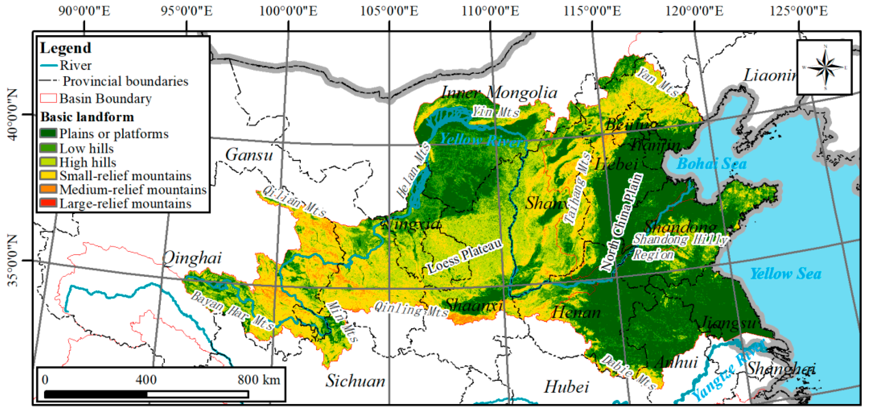
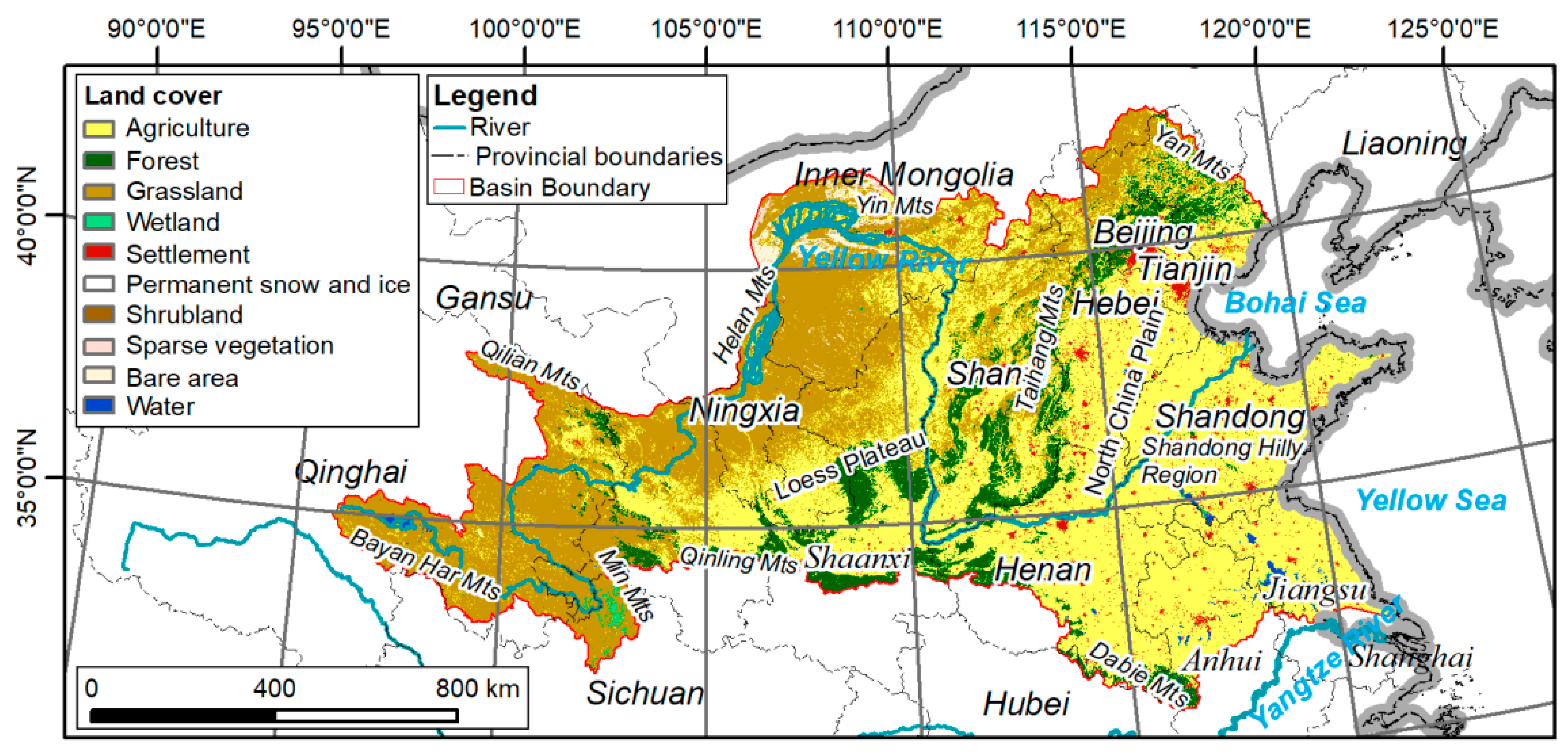
2.1. Study Area

The Yellow River, located in the north-central part of China (Figure 1), is the second-longest river in China, with a total length of 5464 km [26]. It flows through the Qinghai Tibet Plateau, Inner Mongolia Plateau, Loess Plateau, and Huang-Huai-Hai Plain [27], and goes through nine provinces, including Qinghai, Sichuan, Gansu, Ningxia, Inner Mongolia, Shaanxi, Shanxi, Henan, and Shandong [28,29]. The terrain of the Yellow River Basin is high in the West and low in the East [30]. According to statistics, the total area of the Yellow River Basin is 795,000 km² [31,32]. The annual average temperature of the basin is about 7 ℃ and the annual average precipitation is about 440 mm [33]. Now, the Yellow River basin has become one of the most vulnerable areas of ecological environment in China due to its complex landforms and climate differences. Serious water pollution, land desertification, gradual reduction of runoff, intensified soil erosion, and vegetation degradation [34] have become the focus of sustainable development of the Yellow River Basin. On 18 September 2019, the "Ecological protection and high-quality development in the Yellow River River Basin" was upgraded to a major national strategy by the China’s government on a forum in Zhengzhou, Henan, China [35,36].

It should be noted that the Yellow River is a special river which exists in the form of suspended river on the ground in the lower reaches. According to statistics, thousands of years before, and until, 1946, the Yellow River burst 1593 times, and 26 major river diversions occurred [37,38,39]. Among them, the northernmost diversion occupied the Hai River and flowed into the Bohai Sea; the southernmost diversion passed through the Huai River (Figure 1). Considering the particularity of the Yellow River, we believe that the relevant research on the Yellow River cannot be limited to the existing basin, because its lower reaches are bounded by artificial levees and do not show a natural state. Therefore, we selected the Yellow River Basin, the Huai River Basin, and the Hai River Basin, which all are greatly affected by the Yellow River, to form the GYRR (Figure 1), and used them as the research area in response to “ecological protection and high-quality development of the Yellow River Basin”. For the GYRR, relevant scholars have put forward similar concepts, such as the “Great Yellow River theory” of Guo [40], which defines a similar research area to guide relevant researchers to explore the development, evolution, generation, watershed size, source, rheology, estuary, river length, disaster, and contribution of the Yellow River. Mostern [41], in his book “The Yellow River-A Natural and Unnatural history”, also selected a similar study area to introduce many research aspects of the Yellow River, such as history, loess, levies, and levees.

Figure 1. GYRR extent, including the Yellow River Basin, the Huai River Basin, and the Hai River Basin. A similar region concept has been recognized and mentioned by many scholars [40,41]. Historically, the Yellow River has burst and changed its course many times, affecting a wide area. At present, the lower reaches of the Yellow River are overland rivers, which are not natural rivers, but are significantly affected by human activities. Therefore, the study of the Yellow River should consider the history and river characteristics. It is more reasonable to take the area affected by the Yellow River as the study area of the Yellow River. In particular, we propose that historical archaeologists may take this area as the research area for Yellow River civilization archaeology.

Figure 1. GYRR extent, including the Yellow River Basin, the Huai River Basin, and the Hai River Basin. A similar region concept has been recognized and mentioned by many scholars [40,41]. Historically, the Yellow River has burst and changed its course many times, affecting a wide area. At present, the lower reaches of the Yellow River are overland rivers, which are not natural rivers, but are significantly affected by human activities. Therefore, the study of the Yellow River should consider the history and river characteristics. It is more reasonable to take the area affected by the Yellow River as the study area of the Yellow River. In particular, we propose that historical archaeologists may take this area as the research area for Yellow River civilization archaeology.

The GYRR is bounded by the Yanshan and Yinshan Mountains in the north, Helan and Qilian Mountains in the west, Qinling and Dabie Mountains in the South, and Bohai and Yellow Sea in the East. The division of the surrounding mountains causes the GYRR to become an independent geographical unit. The Yellow River, which has changed its course for many times, has become the tie linking different parts of the geographical unit. This area has become the main and core area of the Yellow River civilization. In terms of administrative divisions, the GYRR occupies all of Shandong, Shanxi, and Ningxia, most places in Henan and Hebei, the east part of Qinghai, the middle and north parts of Shaanxi, the north part of Jiangsu and Anhui, the south part of Gansu, the northwest corner of Sichuan, and the middle part of Inner Mongolia. A total of 12 provinces are involved. In terms of geomorphology, the western areas of the GYRR are the mountainous areas, while the eastern part is a large area of alluvial plains. The area percentage of plains and platforms is about 34.96%, and that of mountainous areas is 65.04% (Figure 2).

2.2. Materials

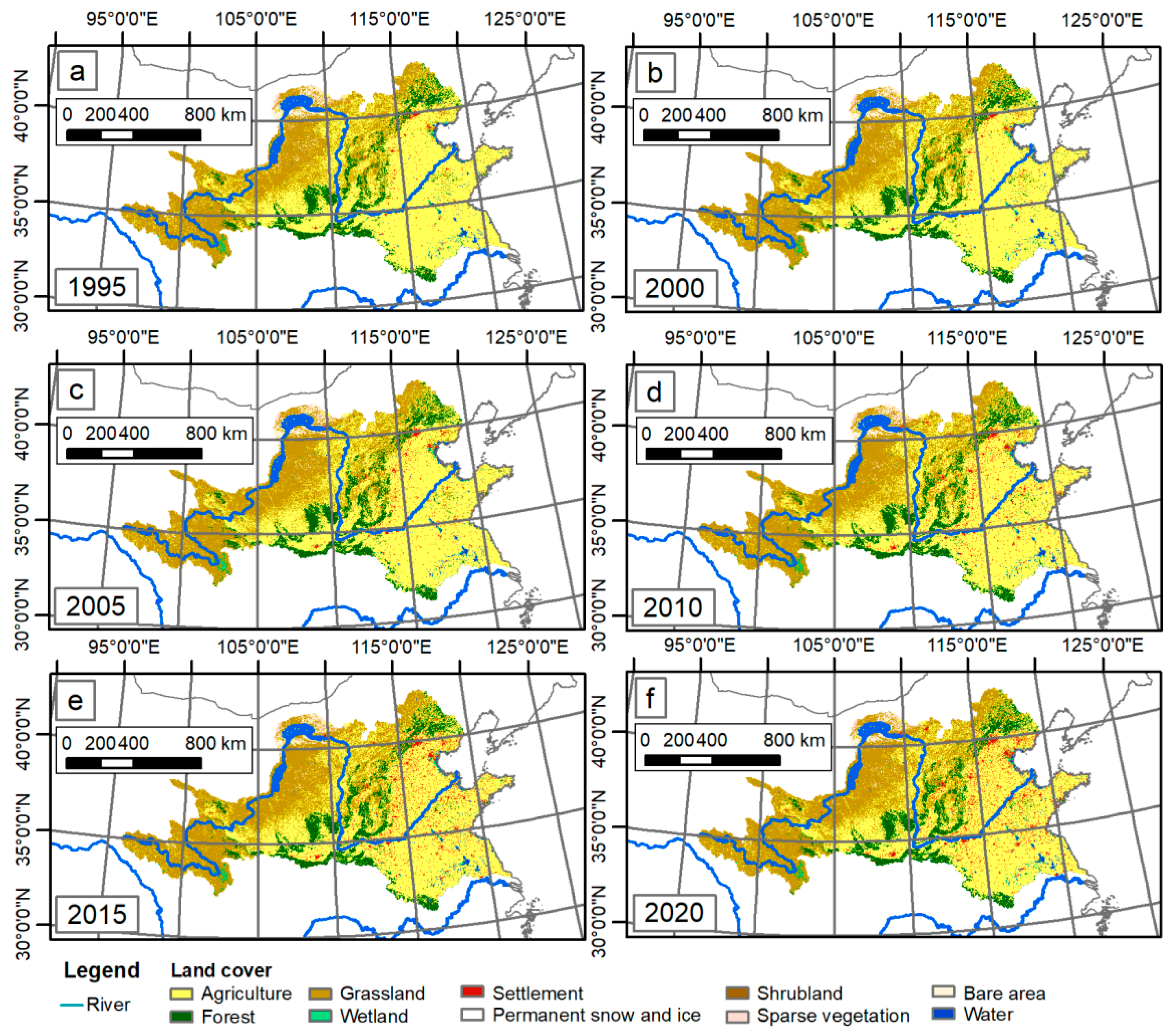
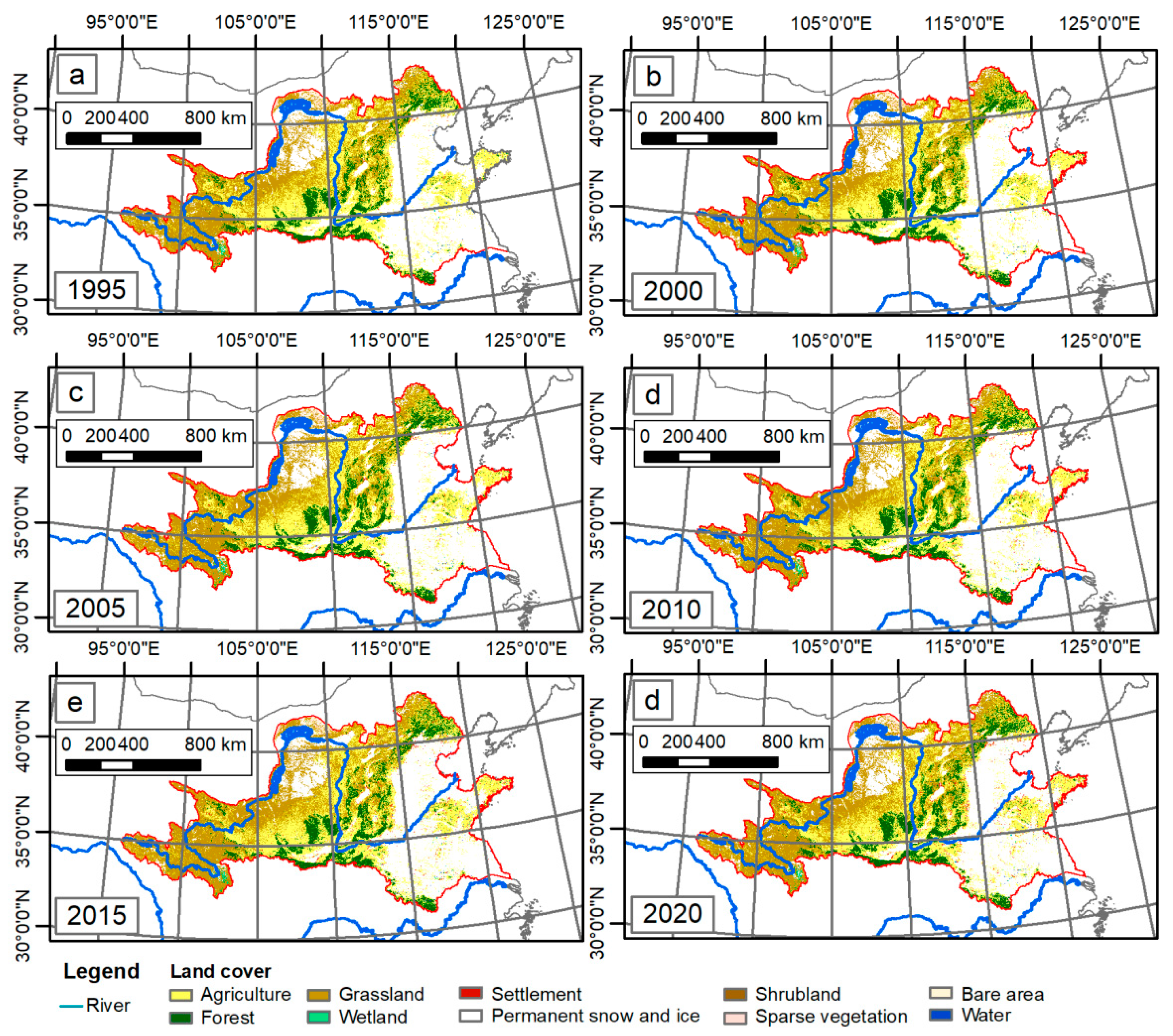
2.2.1. Land Cover Data

The land cover data used in this study (1995, 2000, 2005, 2010, 2015, and 2020) were downloaded from the land cover classification data set released by the European Space Agency (ESA) climate change initiative [42]. The spatial resolution is 300 m. Using the international Intergovernmental Panel on Climate Change (IPCC) land categories, the land cover types were divided into 10 categories: (i) agriculture, (ii) forest, (iii) grassland, (iv) wetland, (v) settlement, (vi) permanent snow and ice, (vii) shrubland, (viii) sparse vegetation, (ix) bare area, and (x) water (Figure 3). We resampled these land cover data and obtained multi-temporal 1000-m resolution land cover data.

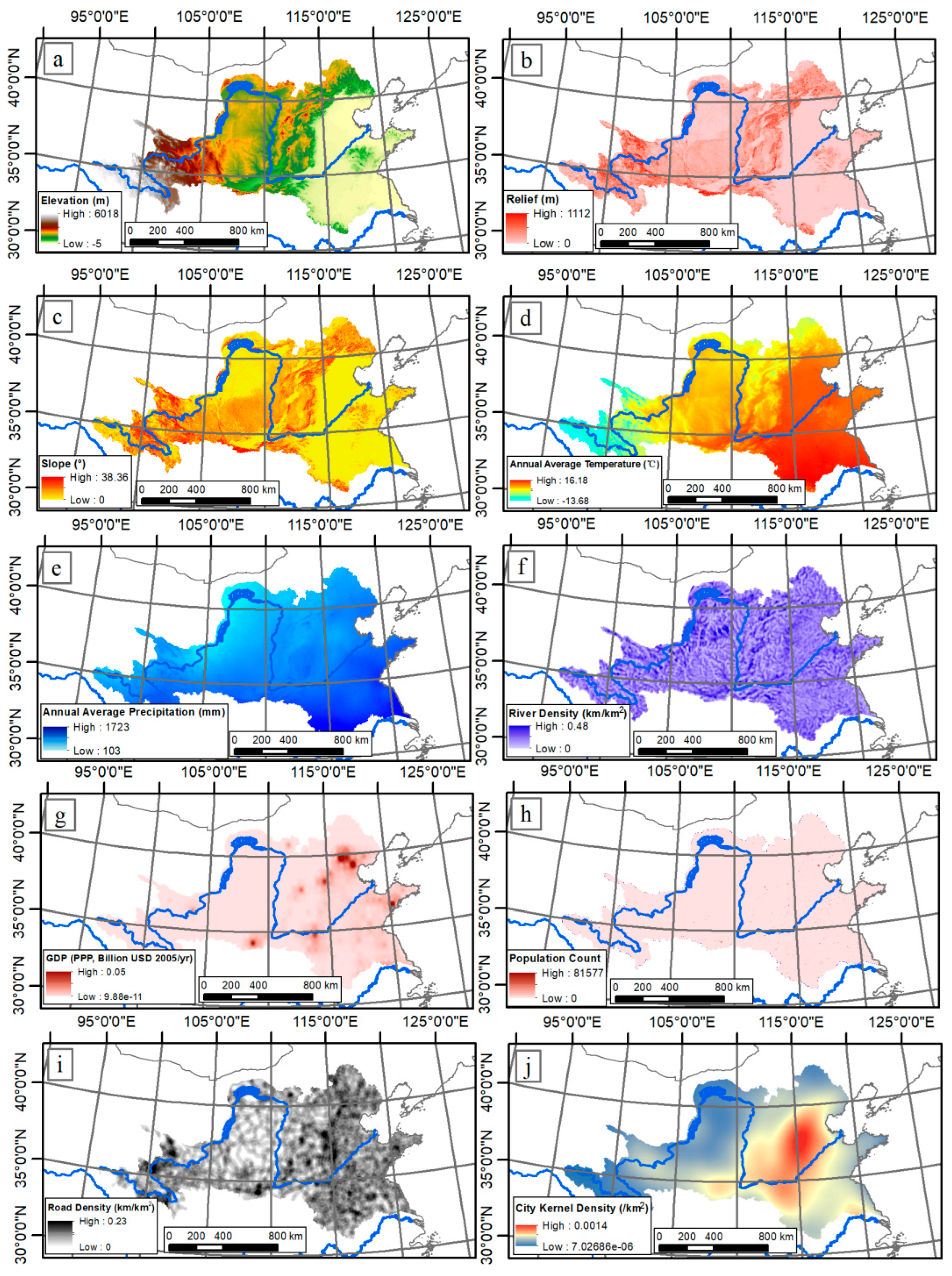
2.2.2. Spatial Variables Affecting the Land Cover Change

Physical and socioeconomic elements may cause alterations in land cover. For the selection of spatial variables affecting land cover change, we mainly referred to the relevant literature [14,43,44,45,46,47,48,49]. After comparison and analysis, we employed a variety of physical and socioeconomic elements (

Table 1. Data sources.

Data	Source	Access Date
Elevation	https://www.earthenv.org/topography [50]	20 May 2022
Relief	Calculated from Elevation	20 May 2022
Slope	https://www.earthenv.org/topography [50]	20 May 2022
Temperature	https://www.worldclim.org/data/index.html [51]	22 May 2022
Precipitation	https://www.worldclim.org/data/index.html [51]	22 May 2022
River	https://www.hydrosheds.org/products/hydrorivers [52]	28 May 2022
GDP	https://www.nies.go.jp/link/population-and-gdp.html [53]	6 June 2022
Population	https://landscan.ornl.gov/ [54]	10 June 2022
Road	https://sedac.ciesin.columbia.edu/data/set/groads-global-roads-open-access-v1/data-download [55]	11 June 2022
City	https://www.resdc.cn/data.aspx?DATAID=211 [56]	15 June 2022

), including the elevation, topographic relief, slope, annual average temperature, annual average precipitation, river network density, GDP, population, road network density, and city density.

The elevation data (Figure 4a) were downloaded from the EarthEnv website (https://www.earthenv.org/topography). We found that the landform of the whole GYRR is high in the west region and low in the east region. There are many mountains in the west, and alluvial plains and hills in the east. The highest altitude of the whole area is 6018 m. The topographic relief was calculated from elevation, and the maximum relief in this region is 1112 m. The high value of relief is mainly distributed in the Taihang Mountains (Figure 4b). The slope data (Figure 4c) were also downloaded from the EarthEnv website (https://www.earthenv.org/topography). The high value distribution of the slope is similar to the relief high value distribution. The maximum value of the slope is 38.36°. The temperature and precipitation data were downloaded from the WorldClim website. WorldClim version 2.1 climate data for 1970–2000 was released in January 2020. They provide monthly climate data for minimum, mean, and maximum temperature, precipitation, solar radiation, wind speed, water vapor pressure, and total precipitation at the four spatial resolutions, between 30 s and 10 min. Each download is a “zip” file that contains 12 GeoTiff (.tif) files, one for each month of the year (January is 1; December is 12). We obtained the annual average temperature by averaging the 12-monthly mean temperature data. It was found that the maximum annual average temperature in this area is 16.18℃ and the minimum is −13.68 ℃ (Figure 4d). Due to the influence of monsoons, the temperature in the East is higher, while the influence of ocean in the West is weak, and the temperature is lower. The precipitation data were also taken from the WorldClim website. We summed up the 12-monthly precipitation data to obtain the annual average precipitation. The precipitation in the GYRR decreases from Southeast to Northwest. The annual maximum precipitation can reach 1723 mm (Figure 4e). The river network density was calculated using the river network data (Figure 4f). In addition, data related to human activities mainly include GDP, population, road density, and city density. Due to the accumulation of human beings in the plain area, the four above-mentioned factors show the characteristics of high density in the plain area (Figure 4g−j).

2.2.3. Mountain Hazards in the GYRR

Mountain hazards generally refer to the hazards that can threaten human beings and their living environment in mountainous areas [57,58]. Tang et al. [59] discussed and defined “mountain hazards” in the 1980s, and considered that landslides, collapses, mudslides, soil erosion, ice avalanches, frozen soil hazards, earthquakes, hail, and other hazards in the mountainous areas could all be classified as mountain hazards. As compared with the above-mentioned broad categories, mountain hazards, in a narrow sense, could be understood as the phenomenon through which the water and soil materials move along the slope under the driving force of gravity and have a certain destructive capacity [60]. Debris flows, landslides, collapses, and mountain torrents are the representatives of common typical mountain hazards. In this study, we collected data on landslides, mountain torrents, and debris flows in the GYRR. For the collection of landslide and debris flow data, the global landslide catalog (GLC) from 2007 to 2017 produced by the National Aeronautics and Space Administration (NASA) of the United States was downloaded to collect rainfall-induced landslide and debris flow events. The data sources of the GLC include media, disaster databases, scientific reports, etc. [61]. On the other hand, the Dartmouth flood Observatory was established in 1993, mainly recording major global flood events from January 1985 [62]. For the mountain torrents, as a special flood occurring in the mountainous areas, the mountainous areas of the GYRR were used to screen the above flood event points and to obtain the mountain torrent points.

2.3. Methods

2.3.1. MOLUSCE Plugin

Asia Air Survey Co., Ltd. (AAS) released MOLUSCE (Modules for Land Use Change Evaluation) at FOSS4G 2013, which was a conference for people working with open-source tools. As a user-friendly plug-in for QGIS 2.0 and above, MOLUSE is designed to analyze, model, and simulate land use/cover changes. MOLUSCE is well suited to analyze land use and forest cover changes between different time periods, model land use/cover transition potential or areas at risk of deforestation, and simulate future land use and forest cover changes [63].

2.3.2. Correlation Analysis

Correlation analysis refers to the analysis of two or more variable elements with correlation, to measure the closeness of the correlation between the variable factors. The measurement of the closeness of the relationship between geographical elements is mainly realized through the calculation and interpretation of the correlation coefficient. Pearson’s correlation and Cramer’s coefficient are the main correlation analysis methods in the MOLUSCE plugin of QGIS. Among them, Pearson correlation analysis is a measurement method of vector similarity [64]. The output range is from −1 to + 1, where 0 represents no correlation, negative value represents negative correlation, and positive value represents positive correlation.

The correlation degree is usually judged by the following value ranges:

• 0.8–1.0: extreme correlation;
• 0.6–0.8: strong correlation;
• 0.4–0.6: moderate correlation;
• 0.2–0.4: weak correlation;
• 0.0–0.2: very weak correlation or no correlation.

2.3.3. Change Analysis and Transition Potential Modeling

We used the MOLUSCE plugin inside QGIS to compute the land cover change between the research intervals. For transition potential modeling, we used the logistic regression approach. The elevation, relief, slope, monthly average temperature, annual average precipitation, river density, GDP, population count, road density, and city kernel density were used as the explanatory factors.

2.3.4. Prediction and Model Validation

The MOLUSCE plugin can not only efficiently compute land cover change analyses, but is also well-suited for simulating future scenarios of land cover. We used the CA Simulation tool [65,66,67] of the MOLUSCE plugin inside QGIS to simulate the future land cover after we finished the transition potential modeling operation using the logistic regression approach. Next, we entered the reference map and simulated map for comparison and verification on the Validation page of the MOLUSCE plugin, and obtained the relevant Kappa coefficient values as a reference to check the accuracy of the simulation results.

2.3.5. Annual Rate of Change Analysis

The annual rate of change (ARC) could be used to represent the magnitude of change between corresponding years. In order to obtain the annual rate of change for each land cover type, the area difference between the final year and initial year was divided by the area of initial year and time (year) period. We used Equation (1) to assess the annual rate of change in land cover categories [25,68]:

$$\mathrm{ARC}=\frac{{\mathrm{Area}}_{\mathrm{Final}}-{\mathrm{Area}}_{\mathrm{Initial}}}{{\mathrm{Area}}_{\mathrm{Initial}}*\mathrm{t}}\times 100\%$$

(1)

where ARC is the annual rate of change in land cover categories. Area_Final and Area_Initial are the areas of final and initial year, and t is the interval of years between the final year and initial year.

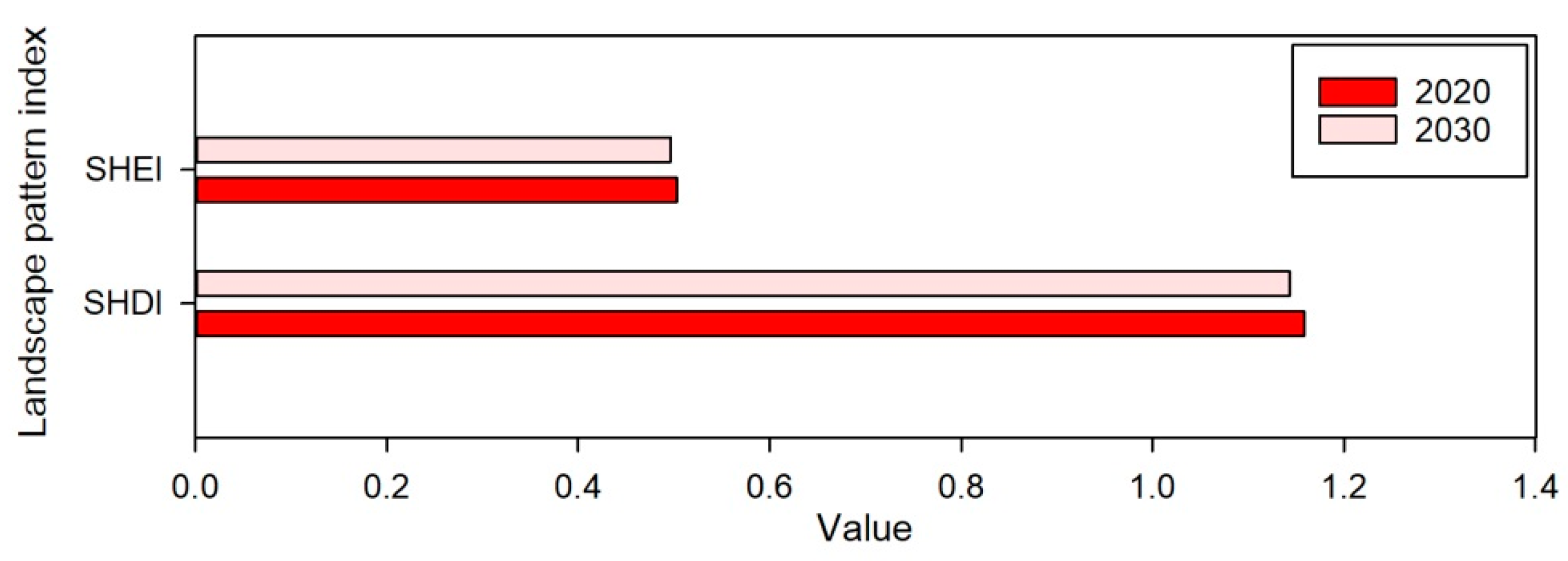
2.3.6. Landscape Pattern Index Analysis

The landscape pattern is the arrangement of landscape blocks of different sizes and shapes formed naturally or artificially in landscape space [69]. The landscape pattern indexes, as the sub-classification of landscape indexes, reflect the structural characteristics of land use/land cover types [70]. There are many types of landscape pattern indexes, and because of the application of new theories in landscape ecology, they are constantly being pushed forward [71,72]. Researchers often extend this part of the functions of the Geographic Information System (GIS) to form a unique landscape index software package based on GIS, such as Fragstats software package.

In order to study the spatial structure characteristics of different land cover types in the GYRR, this study first introduced the landscape diversity index to characterize them. Shannon’s Diversity Index (SHDI) is a measurement index which is widely used in ecology based on information theory, and it is equal to the negative sum of the area ratio of each patch type multiplied by the natural logarithm of its value at the landscape level:

$$\mathrm{SHDI}=-{\displaystyle \sum }_{i=1}^s{P}_{i}ln{P}_i$$

(2)

where s is the amount of patches, and P_i the area ratio of each patch type. When SHDI = 0, it indicates that the whole landscape is composed of only one patch, and an increase in SHDI indicates that the patch types increase or distribute equally in the landscape space. In a landscape system, the richer the land use/land cover is, the higher the degree of fragmentation is, and more uncertain information content leads to a higher calculated SDHI value. The diversity depends on two factors: the number of types and the evenness of area combination; therefore, the diversity index is the comprehensive embodiment of type richness and combination complexity [73].

Shannon’s Evenness Index (SHEI) equals the SHDI divided by the maximum possible diversity under a given landscape abundance (all patch types are equally distributed). The smaller the SHEI value is, the more likely it is that some patch types may dominate the landscape, and a value that is close to 1 indicates that there is no obvious dominant type in the landscape while patch types are evenly distributed. Therefore, when SHEI = 0, it indicates that the landscape is composed of only one type of patch without diversity, and SHEI = 1 indicates that the patches are evenly distributed and have the greatest diversity.

$$\mathrm{SHEI}=\frac{SHDI}{SHD{I}_{max}}$$

(3)

where SHDI is Shannon’s Diversity Index, and SHDI_max is the maximum possible diversity under a given landscape abundance (all patch types are equally distributed) [74].

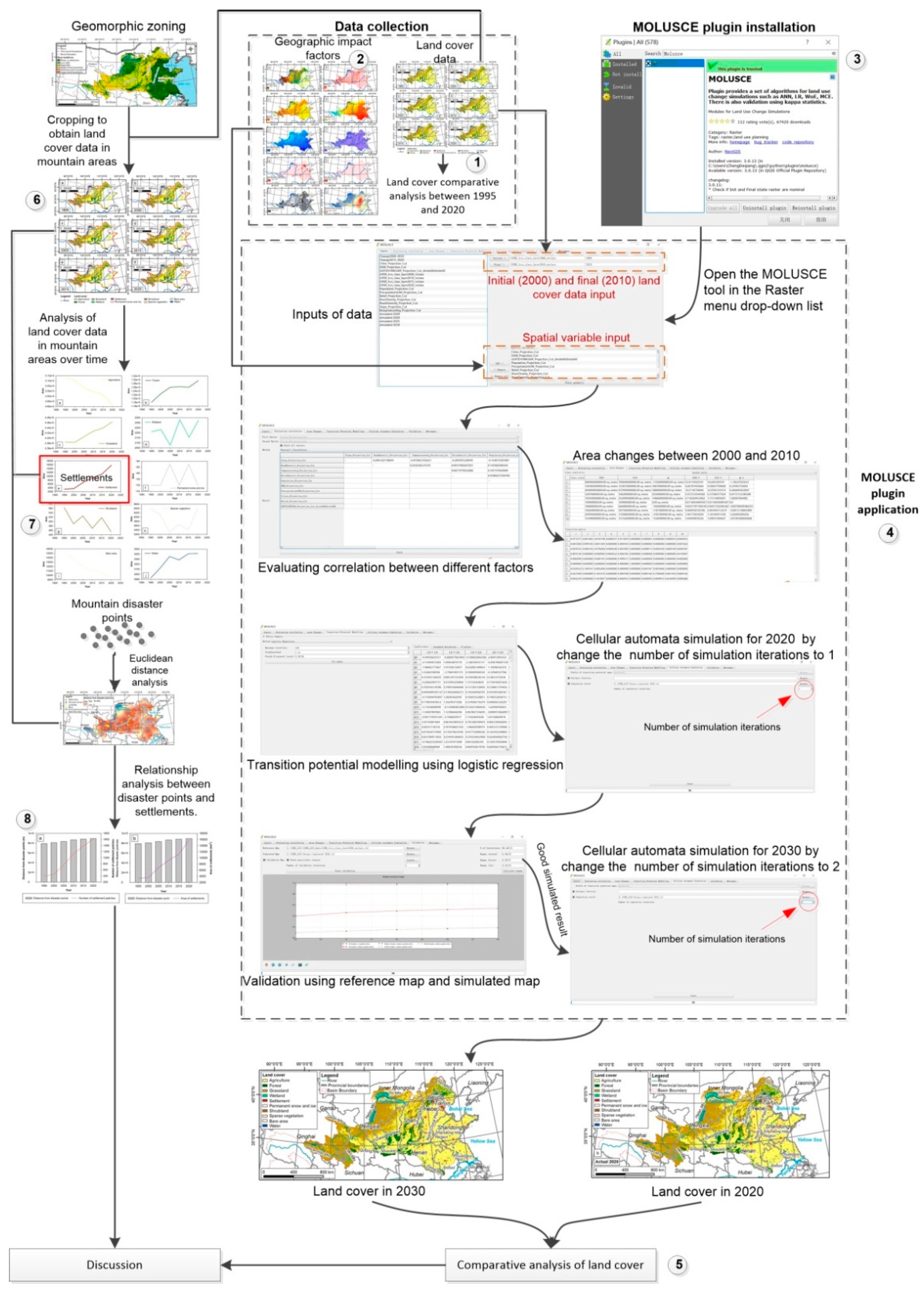
2.4. Technology Roadmap

In the process of this research, our work includes the following steps (Figure 5):

(1) We downloaded the land cover data for six years, including 1995, 2000, 2005, 2010, 2015, and 2020, and then, by comparing and analyzing the data of the first year (1995) and the last year (2020), we gained general insight into the land cover change in the GYRR in the past 25 years.

(2) The data of 10 geographical elements from different data sources, including elevation, relief, slope, annual average temperature, annual average precipitation, river network density, GDP, population, road density, and city density were collected.

(3) The MOLUSCE plugin was found in the plugin installation window and installed.

(4) We opened the MOLUSCE tool in the Raster menu drop-down list. Initial (2000) and final (2010) land cover data were used as input. Geographic impact factors, such as spatial variable, were used as input in the “inputs” tab of the MOLUSCE tool. Then, the subsequent operations were carried out step by step. The data generated in the previous step were the basis for the next operation. In particular, we carried out the prediction of land cover in 2030 after verifying the effectiveness of the prediction model.

(5) By comparing the land cover data in 2020 and 2030, we analyzed the land cover change over the next 10 years.

(6) On the other hand, we used the mountainous areas of the GYRR to cut out the land cover data of six periods from 1995 to 2020.

(7) The area changes in different land cover types in the mountainous areas of the GYRR were analyzed over time.

(8) Mountain hazard data points were downloaded and sorted to conduct the Euclidean distance analysis. The relationship analyses include distance from hazard points, number of settlement patches, distance from hazard points, and area of settlements.

3. Results

3.1. Correlation between Geographical Variables

We calculated the Pearson correlation coefficient, as shown in

Table 2. Pearson correlation coefficient between different variables.

	Temperature	Road Density	Elevation	GDP	City Density	Slope	Population	Relief	River Density	Precipitation
Temperature		0.26	−0.95	0.35	0.68	−0.48	0.19	−0.48	0.09	0.48
Road Density			−0.27	0.30	0.32	−0.20	0.15	−0.15	0.09	0.19
Elevation				−0.37	−0.64	0.49	−0.17	0.49	−0.07	−0.34
GDP					0.37	−0.24	0.19	−0.22	0.06	0.17
City Density						−0.19	0.17	−0.19	0	0.35
Slope							−0.15	0.87	−0.21	−0.05
Population								−0.14	0.04	0.12
Relief									−0.19	−0.07
River Density										−0.12
Precipitation

. After comparison, it was found that the variables having strong correlation with each other include temperature and elevation, city density and temperature, city density and elevation, and relief and slope.

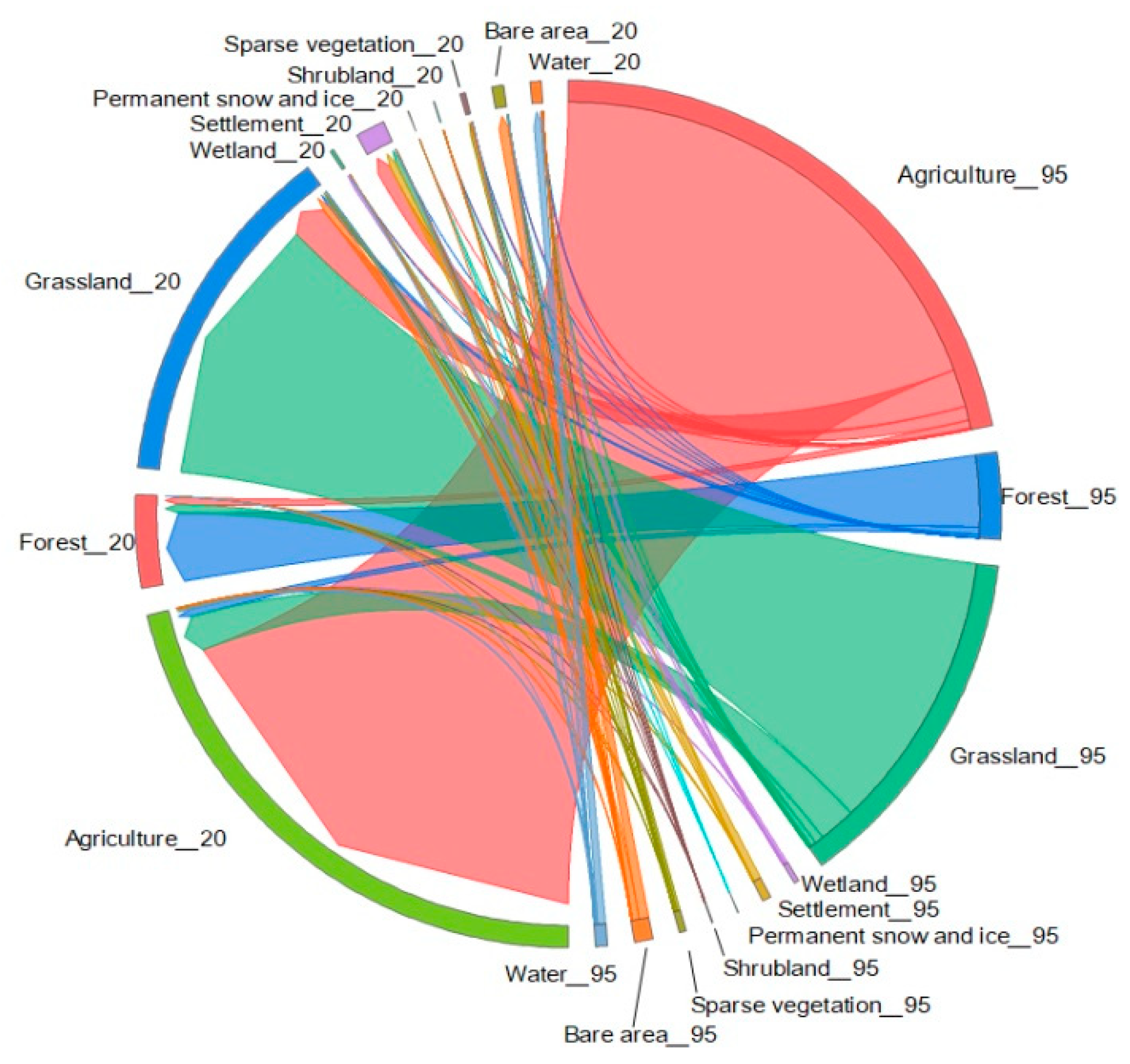
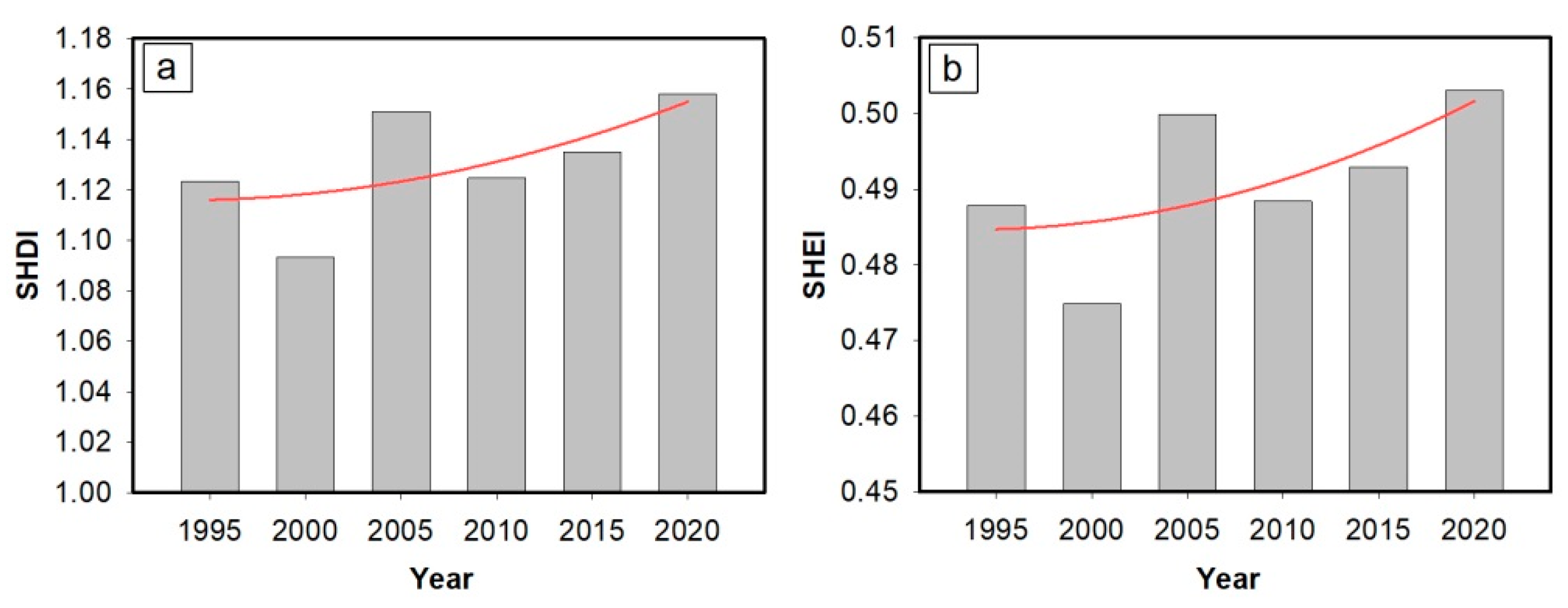
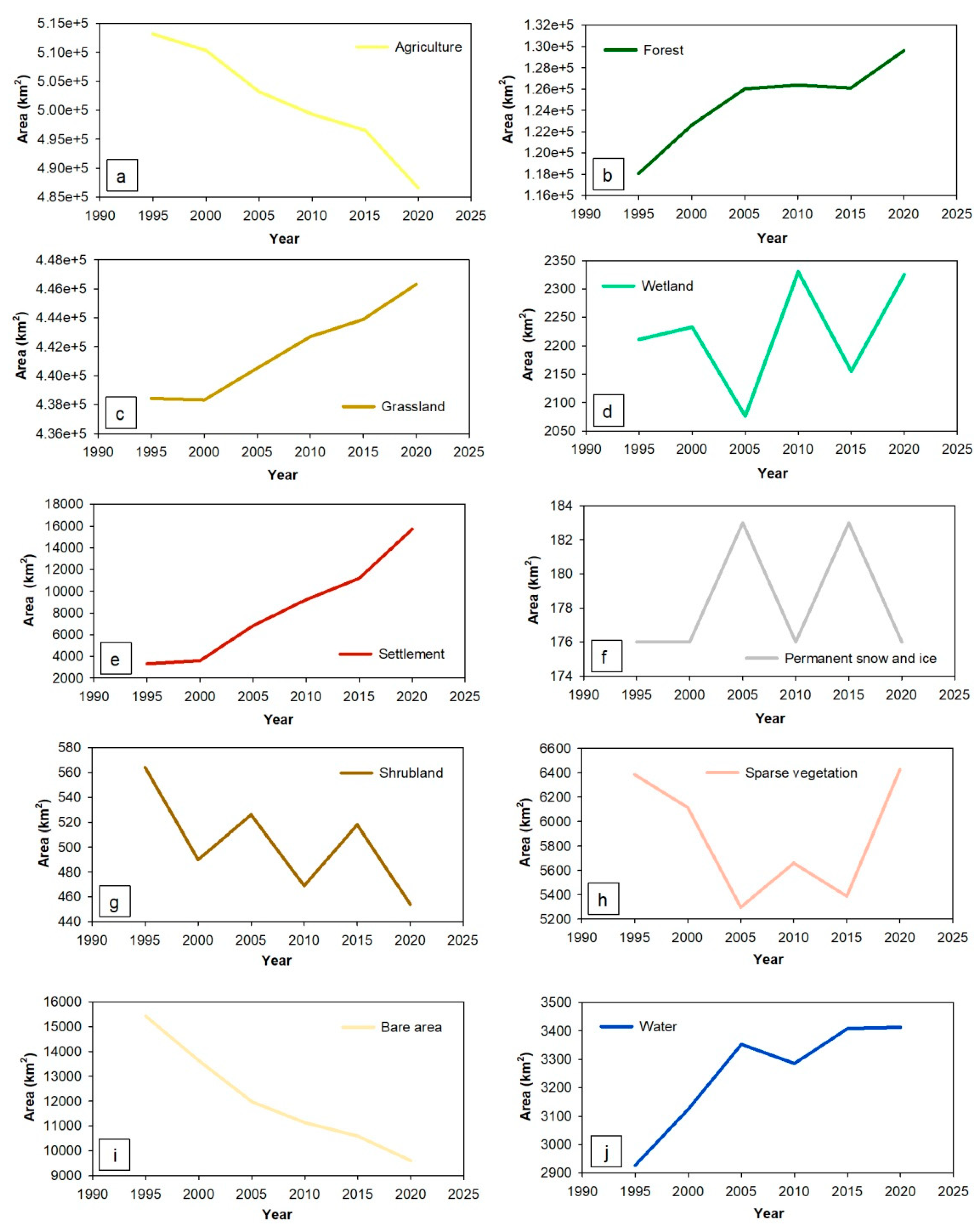
3.2. Area Changes and Landscape Pattern Features

The statistical analysis was done on various land cover areas between 1995 and 2020. The area change and the ARC of the same land cover were calculated (

Table 3. Land cover change from 1995 to 2020.

Land cover type	Area in 1995 (km2)	Area in 2020 (km2)	Area change (km2)	ARC
Agriculture	788,382	771,945	−16,437	−0.08%
Forest	116,638	126,528	+9890	+8.48%
Grassland	476,334	474,525	−1809	−0.38%
Wetland	7005	5410	−1595	−22.77%
Settlement	12,233	39,597	+27,364	+223.69%
Permanent snow and ice	178	169	−9	−5.06%
Shrubland	1257	646	−611	−48.61%
Sparse vegetation	8662	6681	−1981	−22.87%
Bare area	25,027	15,683	−9344	−37.34%
Water	16,126	15,024	−1102	−6.83%

). It was noted that the land cover with the largest change was agricultural land, with a decrease of −16,437 km². The increase in settlement area is the largest one, with an area of +27,364 km² and an ARC of 223.69%. The increase in settlement shows the enhancement of human activities in the past 25 years.

The area transfer analysis was also performed between different land cover types. According to the area transfer matrix (

Table A1. Area transfer matrix between land cover in 1995 and land cover in 2020.

Land Cover Type		2020 (km2)
		Agriculture	Forest	Grassland	Wetland	Settlement	Permanent Snow and Ice	Shrubland	Sparse Vegetation	Bare Area	Water	SUM
1995 (km2)	Agriculture	701,727	11,171	53,366	287	20,047	2	36	174	118	1454	788,382
	Forest	10,233	101,506	4562	8	123	0	12	1	5	188	116,638
	Grassland	52,088	12,597	399,627	478	7645	10	61	943	1744	1141	476,334
	Wetland	1224	0	1083	4015	206	0	0	0	6	471	7005
	Settlement	1675	7	62	3	10,473	0	0	0	0	13	12,233
	Permanent snow and ice	0	0	32	0	0	145	0	0	1	0	178
	Shrubland	140	456	94	0	9	0	420	106	26	6	1257
	Sparse vegetation	683	2	3358	2	64	0	77	4215	223	38	8662
	Bare area	481	2	9681	9	246	5	40	1101	13,437	25	25,027
	Water	2710	81	945	546	592	0	0	67	16	11,169	16,126
	SUM	771,945	126,528	474,525	5410	39,597	169	646	6681	15,683	15,024	1,456,208

), between 1995 and 2020, large change situations include: 11,171 km² agricultural land was transformed into forest land, 53366 km² agricultural land was transformed into grassland, and 20,047 km² agricultural land was transformed into settlement land. In terms of forest land, 10,233 km² forest land was transformed into agricultural land, and 101,506 km² forest land was transformed into grassland. On the other hand, 52,088 km² grassland was transformed into agricultural land, 12,597 km² grassland was transformed into forest land, and 7645 km² grassland was transformed into settlement land. The Chord diagram (Figure 6) was used to express the land cover change. It was found that agriculture, grassland, and forest are the main land cover types, and account for most of the land studied.

We analyzed the landscape pattern indexes SHDI and SHEI in the GYRR, and the values of the two indexes increased gradually with time (Figure 7). The continuous increase in the SHDI value indicate that the land cover in the GYRR had become more and more abundant, and the higher the degree of fragmentation was, the greater the uncertain information content became. SHEI was getting bigger and bigger, approaching 1, which indicated that there was no obvious dominant type in the GYRR, and landscape patches were more and more evenly distributed in the GYRR.

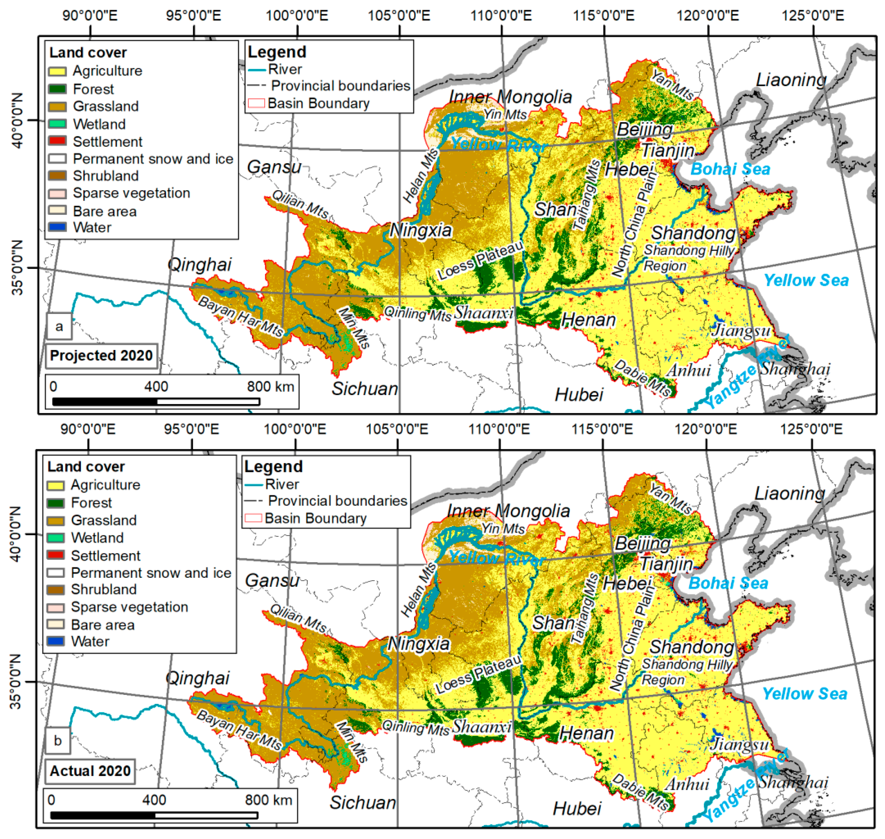
3.3. Land Cover Prediction in 2020 and Validation

We used the MOLUSCE plugin for the simulation of land cover in 2020. Using the projected 2020 data (Figure 8a) for comparison with the actual land cover data in 2020 (Figure 8b), the percentage of correctness was calculated as 96.42%, the Kappa (overall) was 0.94, the Kappa (histo) was 0.98, and the Kappa (loc) was 0.95. The results show that the 10-year interval prediction model has a good result on land cover simulation and prediction.

3.4. Land Cover Prediction in 2030

The above experimental results show that the 10-year interval land cover prediction model has good results. At the windows “Cellular Automata Simulation”, the results show the option “Number of Simulation iterations”. This means that, if only 1 is entered, it will be projected into the future only once. For example, if the land cover data are for 2000 and 2010, the land cover of 2020 will be projected when entering 1, and 2030 will be projected in the case of changing the “Number of Simulation iterations” to 2. In this study, the actual land cover in 2020 was used as the input of the model to simulate and predict the land cover in 2030 (Figure 9).

According to the statistical results of various land cover types, agricultural land, wetland, permanent snow and ice, shrubland, and sparse vegetation would be further reduced. The area of forest, grassland, settlement, bare area, and water would increase (

Table 4. Land cover change from 2020 to expected 2030.

Land Cover Type	Area in 2020 (km2)	Area in 2030 (km2)	Area Change (km2)	ARC
Agriculture	771,945	767,522	−4423	−0.57%
Forest	126,528	129,153	2625	2.07%
Grassland	474,525	483,604	9079	1.91%
Wetland	5410	4533	−877	−16.21%
Settlement	39,597	36,983	−2614	6.60%
Permanent snow and ice	169	83	−86	−50.89
Shrubland	646	533	−113	−17.49%
Sparse vegetation	6681	4282	−2399	−35.91
Bare area	15,683	16,287	604	3.85%
Water	15,024	13,228	−1796	11.95%

).

In particular, it can be noted that a large amount of agricultural land would still turn into grassland and settlement. Some settlement land would be converted into agricultural land and grassland (

Table A2. Area transfer matrix between land cover in 2020 and land cover in 2030.

Land Cover Type		2030 (km2)
		Agriculture	Forest	Grassland	Wetland	Settlement	Permanent Snow and Ice	Shrubland	Sparse Vegetation	Bare Area	Water	SUM
2020 (km2)	Agriculture	747,492	1457	15,042	4	7718	0	5	60	70	97	771,945
	Forest	1911	123,088	1421	0	97	0	3	0	0	8	126,528
	Grassland	8075	4273	459,873	9	966	0	1	162	1057	109	474,525
	Wetland	76	17	193	4342	622	0	0	2	0	158	5410
	Settlement	9490	61	3273	132	26,431	0	6	29	50	125	39,597
	Permanent snow and ice	86	0	0	0	0	83	0	0	0	0	169
	Shrubland	3	52	71	0	0	0	510	3	7	0	646
	Sparse vegetation	64	45	1789	0	3	0	8	4014	707	51	6681
	Bare area	36	9	1240	0	4	0	0	5	14,388	1	15,683
	Water	289	151	702	46	1142	0	0	7	8	12,679	15,024
	SUM	767,522	129,153	483,604	4533	36,983	83	533	4282	16,287	13,228	1,456,208

). On the other hand, we analyzed the change in landscape pattern index (SHDI and SHEI) and found that the two indexes did not change much (Figure 10). This result shows that the land cover change in the GYRR may enter a stable development stage when it reaches a certain degree in the future.

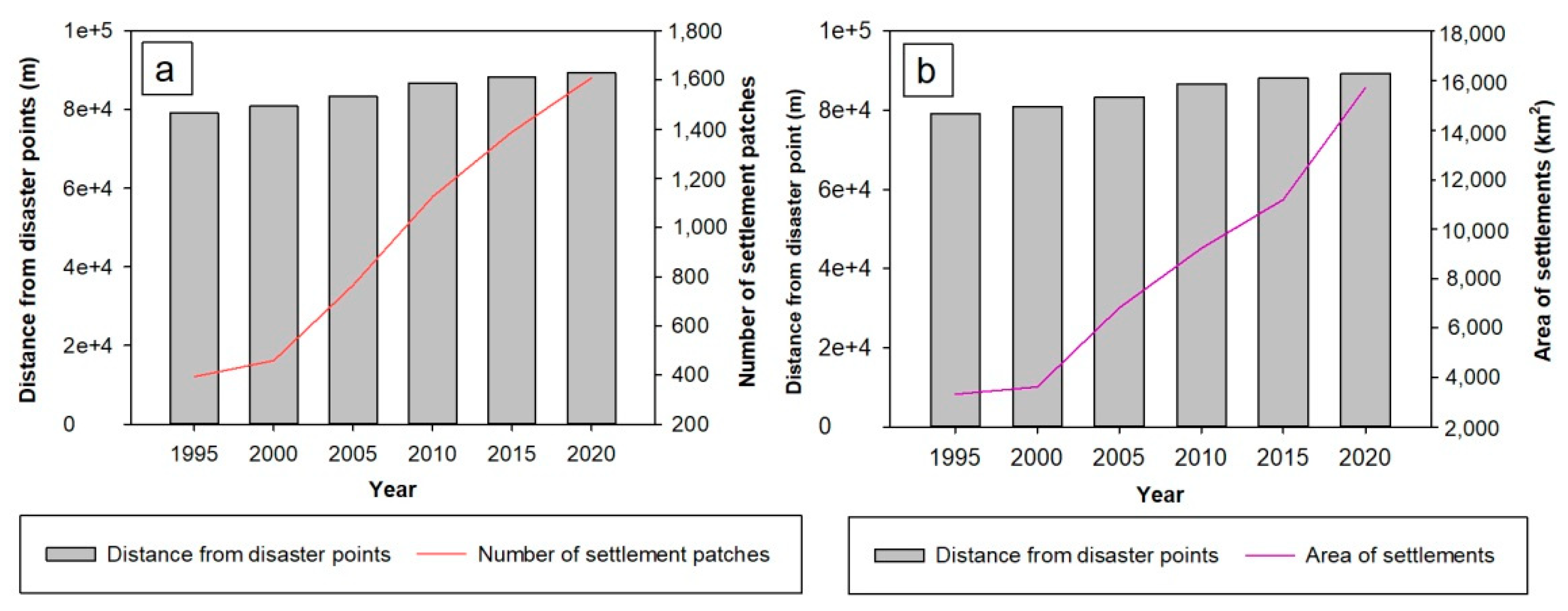
3.5. Land Cover Change in Mountainous Areas

For the whole GYRR, the area percentage of plains and platforms is about 34.96%, and that of mountainous areas is 65.04% (Figure 2). The unique energy gradient causes the mountains to become an area of natural hazards development, such as debris flows, landslides, collapses, avalanches, soil erosion, and mountain torrents. These mountain hazards may destroy urban and rural settlements, damage roads, bridges, and engineering facilities, bury farmlands and forests, and block rivers and reservoirs. They may cause huge casualties, property losses, and ecological damage, seriously threaten the lives and property of the people in the mountainous areas and the safety of engineering construction, and restrict the development of resources and economy in the mountainous areas [60]. We cropped out the land cover of the mountainous areas of the GYRR in different years (Figure 11).

Blind expansion of cities in mountainous areas can easily cause mountain hazards. It would cause huge losses to the life, property, and safety of urban residents. For example, on 14 August 2017, a devastating geo-hazard chain—debris slide, debris flow, and sediment-laden flood—occurred in Freetown, Sierra Leone, resulting in at least 500 deaths, more than 600 missing, and hundreds of houses destroyed. Although rainfall was a trigger factor for the Sierra Leone disaster, rapid and haphazard urbanization increased the hazard and vulnerability [75]. The development of mountain towns is generally affected by many factors such as social economy, topography, and geomorphology. Compared with plain towns, their infrastructure is relatively weak. In particular, poor urban planning and inadequate consideration of risks could lead to the construction of housing in dangerous areas. On the other hand, the removal of hillside vegetation increases erosion potential; low cost buildings using fragile building materials and methods could lack resilience; inadequate risk management leads to weak emergency response.

We have also made area statistics for 10 land cover types (Figure 12). It can be seen that the settlement area in the mountainous areas had been increasing continuously in the past 25 years (Figure 12e), with an ARC value of +14.97%. Thanks to the policy of returning farmland to forests and grasslands implemented by the Chinese government in mountainous areas, the area of ecological land such as forest land and grassland had been continuously increased and, at the same time, the ecological environment had been improved as a gratifying result (Figure 12b,c).

We superimposed landslide, debris flow, and mountain torrent points on the base map of the GYRR (Figure 13). It was found that the mountain-hazard points are mainly distributed in the Central and Western regions of the GYRR. Next, the Euclidean distance is calculated using these mountain-hazard point data in order to represent the distance from the hazard point (Figure 13).

We made the statistics on the number of settlement patches, area of settlements in the mountainous areas of the GYRR, and the average Euclidean distance from the hazard points during the period from 1995 to 2020 with a time interval of five years (Figure 14). According to the statistical results, when the number of settlement patches in mountainous areas continued to increase, the distance between settlements in the GYRR and hazard sites was also increased (Figure 14a). On the other hand, the mountainous residential areas in the GYRR also increased; however, the distance from the hazard point was also increasing (Figure 14b). The above two situations show that, although the intensity of human development in the mountains of the GYRR had been increasing, the awareness of avoiding hazards was also improved.

4. Discussion

4.1. Decrease of Farmland and the Increase of Woodland under Returning Farmland to Forest and Grassland

In 1998, Wuqi County of Yan’an, Shaanxi, China began to forbid grazing on the mountains [76]. After that, this small county, located in the northwest of the GYRR, began to take the lead in implementing the policy of returning farmland to forests [77]. Since 1999, Yan’an has reached a forest coverage rate of more than 50% and a vegetation coverage rate of more than 80% by returning farmland to forest over more than 20 years [78]. This is only a microcosm of China’s project of returning farmland to forest and grassland. From 1999 to 2013, a total of 298,000 km² farmland in China was returned to forest. The project covers 2279 counties, with 32 million farmers and 124 million farmers directly benefiting. The central government of China has invested 64.7 billion dollars in the project of returning farmland to forest [79]. From 2014 to 2018, the new round of returning farmland to forest and grassland involved 25 provinces (regions) including Hebei, Shanxi, Inner Mongolia, and others [80]. The Loess Plateau of the GYRR was one of the earliest regions to implement the project of returning farmland to forest and grassland which has made great contributions to the improvement of forest coverage in China [81]. Returning farmland to forest and grassland provides a reasonable explanation for the reduction in farmland and the increase of forest land in the GYRR.

4.2. Urbanization in Mountainous Areas of China

Mountainous areas account for 24% of the earth’s land area, and more than 12% of the world’s population lives in mountainous areas [82,83]. China has a large number of mountains. The mountainous areas accounts for about 70% of the land area, and the population accounts for about 45% of the total population of the country. Due to the geographical and economic marginality of mountainous areas, the overall level of urbanization development in mountainous areas is far lower than the average level of China. The low level of urbanization and the slow urbanization process in mountainous areas, and a large number of agricultural population gathered in mountainous areas, will certainly bring great pressure to the ecological environment in mountainous areas. Among China’s 1429 county-level administrative units in mountainous areas, 54% of the counties have an urbanization rate of less than 20%, and only 10% have an urbanization rate of more than 40% [84]. The development of natural resources, especially mineral resources, has played a significant role in promoting the urbanization of mountainous areas, and a number of resource-based cities have emerged. Tourism is a potential tool to promote the diversified development of mountain economy, increase the employment of mountainous residents, alleviate the poverty in mountainous areas, promote the participation of mountainous areas in economic globalization activities, and correct the development gap in mountainous areas. In recent years, tourism has become a new driving force to promote the urbanization of mountainous areas, such as Emeishan City, Wuyishan City, Tai’an City, and Jiuzhaigou County, and other counties and cities have developed rapidly through tourism. At the same time, due to the lack of management and the lag in planning, some mountainous tourism cities have also experienced excessive urbanization [85]. Compared with plain towns, the urban planning in mountainous areas of China seriously lags behind the urban construction. At present, low-level spread of built-up areas and inefficient use of land are common in urban construction in mountainous areas. The level of urban functional layout is not clear. Especially with the increase in population and the shortage of construction land, the important functional layout of mountain towns basically ignores the avoidance of mountain hazards, and the ability of disaster prevention and mitigation is weak. For example, the area which was most seriously affected by the huge debris flow in Zhouqu, Gansu Province happened to be the most densely-populated and prosperous area [86,87]. The development of mountain towns in the GYRR also faces the above problems, accompanied by the increase in the area of residential areas and the number of residential patches.

4.3. Harmonious and Sustainable Development of People and Land in Mountainous Areas

The development of urbanization in mountainous areas should also be compatible with the resources and be coordinated with the land space and environmental capacity [88]. People should adhere to the fundamental support of ecological industry and form an intensive and ecological development model in order to improve the quality of urbanization. It is necessary to change the traditional direction and mode of urbanization development, gradually lead the urbanization construction to the road of new urbanization, implement the green development strategy, intensively utilize resources, improve resource efficiency, promote the intensive utilization of water, soil, and energy resources, and accelerate the construction of resource-saving cities and towns [89]. The development of urbanization in mountainous areas cannot ignore the restrictions of and close relationship with the mountainous environmental factors. We must grasp the basic characteristics and laws of the mountainous environment from different scales and regional differences, and deeply analyze the typical examples of the pattern, resources, and environmental characteristics, as well as the process of urbanization in mountainous areas. At present, the GYRR is carrying out the urbanization of the mountainous areas with an ARC value of +14.97%. There are many problems that need to be seriously considered to minimize the ecological problems caused by the rapid urbanization of the mountainous areas and realize the harmonious and sustainable development of the relationship between people and land in the mountainous areas.

4.4. Keeping Away from Hazards Benefitting from Disaster Prevention and Mitigation in Mountainous Areas of China

China’s mountains account for more than two-thirds of the total land area. With the rapid growth of population and inappropriate production activities in mountainous areas, mountain hazards occur frequently, and people have been disturbed and destroyed by mountain hazards in the process of utilization in mountainous areas [90]. Since the 1960s, China’s relevant departments have begun to carry out the investigation and control of mountain hazards. For example, the color scientific and educational film "debris flow," released in 1965, brought the debris flow phenomenon onto the screen, which played a very strong role in publicizing and popularizing debris flow knowledge [91]. At present, many departments and colleges in China have trained many professional scientific and technological workers in theoretical research and disaster mitigation-prevention practice regarding mountain-hazards, and laid down a solid foundation in theoretical and technical reserves, becoming a very active scientific and technological force in China [92,93]. On the other hand, China has integrated the study of debris flows, landslides, floods, and other hazards, combined the construction of the large environment with the management of small watersheds, carried out comprehensive research on the process of various hazards, implemented comprehensive disaster mitigation, scientifically assessed the current situation and trend of hazards, and put forward quantitative indicators [94]. With the increasing awareness of disaster prevention and mitigation in mountainous areas, although the proportion of residential areas and the number of residential patches in mountainous areas continue to increase, the safety of residential areas in mountainous areas has been continuously improved due to the conscious distance from mountain hazard points of urban construction [95].

5. Conclusions

In this study, the GYRR was selected as the research area. The land cover change analysis, as well as simulation and prediction of future land cover, was performed, focusing especially on the analysis of the relationship between land cover in mountainous areas and mountain hazards. This work verifies that the MOLUSCE plug-in could be effectively applied to land cover simulation on a large regional scale. Based on the analysis in the current study, the following conclusions are drawn:

(1) Based on multi-period land cover data and physical and socioeconomic factors, the logistic regression and CA model within the MOLUSCE plugin in QGIS software was used to perform the future simulation of land cover in the GYRR. This could provide a reference for related research, especially for large regional-scale land cover simulation.

(2) The decrease in farmland and the increase in forest land illustrate the efforts made by the government and residents of the GYRR in improving the ecological environment during the past 25 years.

(3) According to the simulation and prediction results for land cover in 2030, the agricultural land will decrease, and the forest land will increase. At the same time, the increase in land cover in residential areas could not be ignored, which indicates the continuous development of urbanization in the GYRR. On the other hand, landscape pattern index analysis shows that the land cover in the GYRR may enter a roughly stable development stage when it reaches a certain degree in 2030.

(4) Returning farmland to forest and grassland in the GYRR is conducive to ecological improvement. On the other hand, although the residential areas in mountainous areas were built as far away as possible from the mountain hazard points during construction, there could be a problem of rapid and haphazard urbanization, which should also be paid attention to.

References

1. Houghton, R.A. The worldwide extent of land-use change. BioScience 1994, 44, 305–313. [Google Scholar] [CrossRef]
2. Tumer, B.; Meyer, W.; Skole, D. Global land use/land cover change: Toward an integrated program of study. Ambio 1994, 23, 91–95. [Google Scholar]
3. Anderson, J.R. Land use and land cover changes. A framework for monitoring. J. Res. By Geol. Surv. 1977, 5, 143–153. [Google Scholar]
4. Meyer, W.B.; Turner, B. Land-use/land-cover change: Challenges for geographers. GeoJournal 1996, 39, 237–240. [Google Scholar] [CrossRef]
5. Wang, H.; Liu, X.; Zhao, C.; Chang, Y.; Liu, Y.; Zang, F. Spatial-temporal pattern analysis of landscape ecological risk assessment based on land use/land cover change in Baishuijiang National Nature Reserve in Gansu Province, China. Ecol. Indic. 2021, 124, 107454. [Google Scholar] [CrossRef]
6. Muchová, Z.; Tárníková, M. Land cover change and its influence on the assessment of the ecological stability. Appl. Ecol. Environ. Res 2018, 16, 2169–2182. [Google Scholar] [CrossRef]
7. Liu, Y.; Wang, D.; Gao, J.; Deng, W. Land use/cover changes, the environment and water resources in Northeast China. Env. Manag. 2005, 36, 691–701. [Google Scholar] [CrossRef]
8. Jianchu, X.; Fox, J.; Vogler, J.B.; Yongshou, Z.P.F.; Lixin, Y.; Jie, Q.; Leisz, S. Land-use and land-cover change and farmer vulnerability in Xishuangbanna prefecture in Southwestern China. Env. Manag. 2005, 36, 404–413. [Google Scholar] [CrossRef]
9. Caldas, M.; Walker, R.; Arima, E.; Perz, S.; Aldrich, S.; Simmons, C. Theorizing land cover and land use change: The peasant economy of amazonian deforestation. Ann. Assoc. Am. Geogr. 2007, 97, 86–110. [Google Scholar] [CrossRef]
10. Lambin, E.F. Modelling and monitoring land-cover change processes in tropical regions. Prog. Phys. Geogr. 1997, 21, 375–393. [Google Scholar] [CrossRef]
11. Cabral, P.; Zamyatin, A. Markov processes in modeling land use and land cover changes in Sintra-cascais, Portugal. Dyna 2009, 76, 191–198. [Google Scholar]
12. Paul, S.; Li, J.; Wheate, R.; Li, Y. Application of object oriented image classification and markov chain modeling for land use and land cover change analysis. J. Environ. Inform. 2018, 31, 30–40. [Google Scholar] [CrossRef]
13. Qiang, Y.; Lam, N.S. Modeling land use and land cover changes in a vulnerable coastal region using artificial neural networks and cellular automata. Environ. Monit. Assess. 2015, 187, 1–16. [Google Scholar] [CrossRef] [PubMed]
14. Liu, X.; Liang, X.; Li, X.; Xu, X.; Ou, J.; Chen, Y.; Li, S.; Wang, S.; Pei, F. A future land use simulation model (flus) for simulating multiple land use scenarios by coupling human and natural effects. Landsc. Urban Plan. 2017, 168, 94–116. [Google Scholar] [CrossRef]
15. Huang, Y.; Yang, B.; Wang, M.; Liu, B.; Yang, X. Analysis of the future land cover change in Beijing using CA–Markov chain model. Environ. Earth Sci. 2020, 79, 1–12. [Google Scholar] [CrossRef]
16. Liu, X.; Wei, M.; Zeng, J. Simulating urban growth scenarios based on ecological security pattern: A case study in Quanzhou, China. Int. J. Environ. Res. Public Health 2020, 17, 7282. [Google Scholar] [CrossRef] [PubMed]
17. Chaudhuri, G.; Clarke, K. The sleuth land use change model: A review. Environ. Resour. Res. 2013, 1, 88–105. [Google Scholar]
18. Han, H.; Yang, C.; Song, J. Scenario simulation and the prediction of land use and land cover change in Beijing, China. Sustainability 2015, 7, 4260–4279. [Google Scholar] [CrossRef] [Green Version]
19. Arsanjani, J.J.; Helbich, M.; Kainz, W.; Boloorani, A.D. Integration of logistic regression, markov chain and cellular automata models to simulate urban expansion. Int. J. Appl. Earth Obs. Geoinf. 2013, 21, 265–275. [Google Scholar] [CrossRef]
20. Kafy, A.-A.; Shuvo, R.M.; Naim, M.N.H.; Sikdar, M.S.; Chowdhury, R.R.; Islam, M.A.; Sarker, M.H.S.; Khan, M.H.H.; Kona, M.A. Remote sensing approach to simulate the land use/land cover and seasonal land surface temperature change using machine learning algorithms in a fastest-growing megacity of Bangladesh. Remote Sens. Appl. Soc. Environ. 2021, 21, 100463. [Google Scholar] [CrossRef]
21. Puangkaew, N.; Ongsomwang, S. Remote sensing and geospatial models to simulate land use and land cover and estimate water supply and demand for water balancing in Phuket island, Thailand. Appl. Sci. 2021, 11, 10553. [Google Scholar] [CrossRef]
22. Li, X.; Chen, G.; Liu, X.; Liang, X.; Wang, S.; Chen, Y.; Pei, F.; Xu, X. A new global land-use and land-cover change product at a 1-km resolution for 2010 to 2100 based on human–environment interactions. Ann. Am. Assoc. Geogr. 2017, 107, 1040–1059. [Google Scholar] [CrossRef]
23. Ren, Y.; Lü, Y.; Comber, A.; Fu, B.; Harris, P.; Wu, L. Spatially explicit simulation of land use/land cover changes: Current coverage and future prospects. Earth-Sci. Rev. 2019, 190, 398–415. [Google Scholar] [CrossRef]
24. Yong, X.; Chuansheng, W. Ecological protection and high-quality development in the yellow river basin: Framework, path, and countermeasure. Bull. Chin. Acad. Sci. 2020, 35, 875–883. [Google Scholar]
25. Abbas, Z.; Yang, G.; Zhong, Y.; Zhao, Y. Spatiotemporal change analysis and future scenario of LULC using the CA-ANN approach: A case study of the greater bay area, china. Land 2021, 10, 584. [Google Scholar] [CrossRef]
26. Xiao, C.; Song, L. Climate Services for the Development Plan of the Yellow River Basin in China. EGU Gen. Assem. 2020, 6231. [Google Scholar]
27. Yuan, Z.; Yan, D.-H.; Yang, Z.-Y.; Yin, J.; Yuan, Y. Temporal and spatial variability of drought in Huang-Huai-Hai river basin, China. Theor. Appl. Climatol. 2015, 122, 755–769. [Google Scholar] [CrossRef]
28. Shao, W.; Yang, D.; Hu, H.; Sanbongi, K. Water resources allocation considering the water use flexible limit to water shortage—A case study in the Yellow River Basin of China. Water Resour. Manag. 2009, 23, 869–880. [Google Scholar] [CrossRef]
29. Lan, H.; Peng, J.; Zhu, Y.; Li, L.; Pan, B.; Huang, Q.; Li, J.; Zhang, Q. Research on geological and surfacial processes and major disaster effects in the Yellow River Basin. Sci. China Earth Sci. 2022, 65, 234–256. [Google Scholar] [CrossRef]
30. Jiang, W.; Yuan, L.; Wang, W.; Cao, R.; Zhang, Y.; Shen, W. Spatio-temporal analysis of vegetation variation in the Yellow River Basin. Ecol. Indic. 2015, 51, 117–126. [Google Scholar] [CrossRef]
31. Yang, T.; Xu, C.Y.; Shao, Q.; Chen, X.; Lu, G.H.; Hao, Z.C. Temporal and spatial patterns of low-flow changes in the Yellow River in the last half century. Stoch. Environ. Res. Risk Assess. 2010, 24, 297–309. [Google Scholar] [CrossRef]
32. Künzer, C.; Ottinger, M.; Liu, G.; Sun, B.; Baumhauer, R.; Dech, S. Earth observation-based coastal zone monitoring of the Yellow River delta: Dynamics in China’s second largest oil producing region over four decades. Appl. Geogr. 2014, 55, 92–107. [Google Scholar] [CrossRef]
33. Tang, Y.; Tang, Q.; Tian, F.; Zhang, Z.; Liu, G. Responses of natural runoff to recent climatic changes in the Yellow River Basin, China. Hydrol. Earth Syst. Sci. Discuss. 2013, 10, 4489–4514. [Google Scholar]
34. Wang, S.; Liu, J.; Yang, C. Eco-environmental vulnerability evaluation in the Yellow River Basin, China. Pedosphere 2008, 18, 171–182. [Google Scholar] [CrossRef]
35. Zhang, X.; Zhou, Y.; Han, C. Research on high-quality development evaluation and regulation model: A case study of the Yellow River water supply area in Henan Province. Water 2023, 15, 261. [Google Scholar] [CrossRef]
36. Chen, Y.; Zhu, M.; Lu, J.; Zhou, Q.; Ma, W. Evaluation of ecological city and analysis of obstacle factors under the background of high-quality development: Taking cities in the Yellow River Basin as examples. Ecol. Indic. 2020, 118, 106771. [Google Scholar] [CrossRef]
37. Shu, L.; Finlayson, B. Flood management on the lower Yellow River: Hydrological and geomorphological perspectives. Sediment. Geol. 1993, 85, 285–296. [Google Scholar] [CrossRef]
38. Wu, H.; Li, X.; Qian, H. Detection of anomalies and changes of rainfall in the Yellow River Basin, China, through two graphical methods. Water 2018, 10, 15. [Google Scholar] [CrossRef] [Green Version]
39. Zhang, R. Morphologic evolution of north china plain and causes of channel changes and overflows of the Yellow River. Geol. Miner. Resour. South China 2000, 4, 52–57. [Google Scholar]
40. Guo, L. A conception about innovating the new Yellow River theory: Dedicated to the centenary of academician Huang Bingwei’s birth and the ninety-five years of academician Wu Chuanjun’s birth. Areal Res. Dev. 2013, 32, 1–5. [Google Scholar]
41. Mostern, R. The Yellow River: A Natural and Unnatural History; Yale University Press: New Haven, CN, USA, 2021. [Google Scholar]
42. ECMWF. Land Cover Classification Gridded Maps from 1992 to Present Derived from Satellite Observations. Available online: https://cds.climate.copernicus.eu/cdsapp#!/dataset/satellite-land-cover?tab=form (accessed on 16 August 2022).
43. Pervez, M.S.; Henebry, G.M. Assessing the impacts of climate and land use and land cover change on the freshwater availability in the Brahmaputra River Basin. J. Hydrol. Reg. Stud. 2015, 3, 285–311. [Google Scholar] [CrossRef] [Green Version]
44. Rutherford, G.N.; Bebi, P.; Edwards, P.J.; Zimmermann, N.E. Assessing land-use statistics to model land cover change in a mountainous landscape in the European Alps. Ecol. Model. 2008, 212, 460–471. [Google Scholar] [CrossRef]
45. Rahman, M.T.U.; Esha, E.J. Prediction of land cover change based on CA-ANN model to assess its local impacts on Bagerhat, southwestern coastal Bangladesh. Geocarto Int. 2022, 37, 2604–2626. [Google Scholar] [CrossRef]
46. Rodríguez Eraso, N.; Armenteras-Pascual, D.; Alumbreros, J.R. Land use and land cover change in the Colombian Andes: Dynamics and future scenarios. J. Land Use Sci. 2013, 8, 154–174. [Google Scholar] [CrossRef]
47. Buğday, E.; Buğday, S.E. Modeling and simulating land use/cover change using artificial neural network from remotely sensing data. Cerne 2019, 25, 246–254. [Google Scholar] [CrossRef]
48. Saputra, M.H.; Lee, H.S. Prediction of land use and land cover changes for north Sumatra, Indonesia, using an artificial-neural-network-based cellular automaton. Sustainability 2019, 11, 3024. [Google Scholar] [CrossRef] [Green Version]
49. Chen, Y.; Li, X.; Liu, X.; Ai, B.; Li, S. Capturing the varying effects of driving forces over time for the simulation of urban growth by using survival analysis and cellular automata. Landsc. Urban Plan. 2016, 152, 59–71. [Google Scholar] [CrossRef]
50. Amatulli, G.; Domisch, S.; Tuanmu, M.-N.; Parmentier, B.; Ranipeta, A.; Malczyk, J.; Jetz, W. A suite of global, cross-scale topographic variables for environmental and biodiversity modeling. Sci. Data 2018, 5, 1–15. [Google Scholar] [CrossRef] [Green Version]
51. Fick, S.E.; Hijmans, R.J. Worldclim 2: New 1-km spatial resolution climate surfaces for global land areas. Int. J. Climatol. 2017, 37, 4302–4315. [Google Scholar] [CrossRef]
52. Lehner, B.; Grill, G. Global river hydrography and network routing: Baseline data and new approaches to study the world’s large river systems. Hydrol. Process. 2013, 27, 2171–2186. [Google Scholar] [CrossRef]
53. NIES. Global Dataset of Gridded Population and gdp Scenarios. Available online: https://www.nies.go.jp/link/population-and-gdp.html (accessed on 6 June 2022).
54. Bright, E.; Coleman, P. Landscan Global 2000, 2000 ed; Oak Ridge National Laboratory: Oak Ridge, TN, USA, 2001. [Google Scholar]
55. Center for International Earth Science Information Network—CIESIN—Columbia University; Information Technology Outreach Services—ITOS—University of Georgia. Global Roads Open Access Data Set, Version 1 (groadsv1); NASA Socioeconomic Data and Applications Center (SEDAC): Palisades, New York, NY, USA, 2013. [Google Scholar]
56. Resource and Environment Science and Data Center. Global Residential Distribution Data. Available online: https://www.resdc.cn/data.aspx?DATAID=211 (accessed on 15 June 2022).
57. Cui, P.; Jia, Y. Mountain hazards in the tibetan plateau: Research status and prospects. Natl. Sci. Rev. 2015, 2, 397–399. [Google Scholar] [CrossRef] [Green Version]
58. Peng, C.; Rong, C.; Lingzhi, X.; Fenghuan, S. Risk analysis of mountain hazards in Tibetan Plateau under global warming. Adv. Clim. Change Res. 2014, 10, 103. [Google Scholar]
59. Tang, B.; Liu, S.; Liu, S. Study on mountain calamities in China. Mt. Res. 1984, 2, 1–7. [Google Scholar]
60. Cui, P. Progress and prospects in research on mountain hazards in China. Prog. Geogr. 2014, 33, 145–152. [Google Scholar]
61. NASA. Global Landslide Catalog Export. Available online: https://data.nasa.gov/Earth-Science/Global-Landslide-Catalog-Export/dd9e-wu2v (accessed on 20 January 2020).
62. Brakenridge, G.R. Global Active Archive of Large Flood Events. Available online: http://floodobservatory.colorado.edu/Archives/ (accessed on 20 December 2019).
63. AAS. Molusce—Quick and Convenient Analysis of Land Cover Changes. Available online: https://nextgis.com/blog/molusce/ (accessed on 20 March 2022).
64. Benesty, J.; Chen, J.; Huang, Y.; Cohen, I. Pearson correlation coefficient. In Noise Reduction in Speech Processing; Springer: Berlin/Heidelberg, Germany, 2009; pp. 1–4. [Google Scholar]
65. Codd, E.F. Cellular Automata; Academic Press: Cambridge, MA, USA, 2014. [Google Scholar]
66. White, R.; Engelen, G. Cellular automata and fractal urban form: A cellular modelling approach to the evolution of urban land-use patterns. Environ. Plan. A 1993, 25, 1175–1199. [Google Scholar] [CrossRef] [Green Version]
67. Guan, D.; Li, H.; Inohae, T.; Su, W.; Nagaie, T.; Hokao, K. Modeling urban land use change by the integration of cellular automaton and markov model. Ecol. Model. 2011, 222, 3761–3772. [Google Scholar] [CrossRef]
68. Muhammad, R.; Zhang, W.; Abbas, Z.; Guo, F.; Gwiazdzinski, L. Spatiotemporal change analysis and prediction of future land use and land cover changes using QGIS MOLUSCE plugin and remote sensing big data: A case study of Linyi, China. Land 2022, 11, 419. [Google Scholar] [CrossRef]
69. Hulshoff, R.M. Landscape indices describing a dutch landscape. Landsc. Ecol. 1995, 10, 101–111. [Google Scholar] [CrossRef]
70. Zhang, Q.; Fu, B.; Chen, L. Several problems about landscape pattern change research. Sci. Geogr. Sin. 2003, 23, 270–275. [Google Scholar]
71. Leitao, A.B.; Ahern, J. Applying landscape ecological concepts and metrics in sustainable landscape planning. Landsc. Urban Plan. 2002, 59, 65–93. [Google Scholar] [CrossRef]
72. Naveh, Z.; Lieberman, A.S. Landscape Ecology: Theory and Application; Springer Science & Business Media: Berlin/Heidelberg, Germany, 2013. [Google Scholar]
73. Yue, W.; Xu, J.; Xu, L.H. An analysis on eco-environmental effect of urban land use based on remote sensing images: A case study of urban thermal environment and NDVI. Acta Ecol. Sin. 2006, 26, 1450–1460. [Google Scholar]
74. Gao, C.; Cheng, L. Tourism-driven rural spatial restructuring in the metropolitan fringe: An empirical observation. Land Use Policy 2020, 95, 104609. [Google Scholar] [CrossRef]
75. Cui, Y.; Cheng, D.; Choi, C.E.; Jin, W.; Lei, Y.; Kargel, J.S. The cost of rapid and haphazard urbanization: Lessons learned from the Freetown landslide disaster. Landslides 2019, 16, 1167–1176. [Google Scholar] [CrossRef] [Green Version]
76. Xin, S.U.; Wang, J.J.; Hui, L.I.; Niu, Y.L. Evolutionary processes in agricultural eco-economic system of Wuqi County after converting slope farmland into forest and grassland. Bull. Soil Water Conserv. 2010, 30, 186–190. [Google Scholar] [CrossRef]
77. Du, Y.; Zhang, D.; Yao, S. Analysis of the driving forces of SLCP based on the weights of evidence model—A case study of Wuqi, Shaanxi Province. Res. Soil Water Conserv. 2017, 24, 325–332. [Google Scholar]
78. Yifan, X.; Shunbo, Y.; Yuanjie, D.; Lei, J.; Yuanyuan, L.; Qing, G. Impact of the ‘grain for green’project on the spatial and temporal pattern of habitat quality in Yan’an city, China. Chin. J. Eco-Agric. 2020, 28, 575–586. [Google Scholar]
79. Zhou, H. Nothing short of a miracle: The two decades’ Chinese restoration of forests and grasslands from farmland. Ecol. Civiliz. World 2019, 10–19. [Google Scholar]
80. Li, S.; Liu, M. The development process, current situation and prospects of the conversion of farmland to forests and grasses project in China. J. Resour. Ecol. 2022, 13, 120–128. [Google Scholar]
81. Ning, J.; Liu, J.; Kuang, W.; Xu, X.; Zhang, S.; Yan, C.; Li, R.; Wu, S.; Hu, Y.; Du, G. Spatiotemporal patterns and characteristics of land-use change in China during 2010–2015. J. Geogr. Sci. 2018, 28, 547–562. [Google Scholar] [CrossRef] [Green Version]
82. Price, M.F. Forests in sustainable mountain development. In Global Change and Mountain Regions; Springer: Berlin/Heidelberg, Germany, 2005; pp. 521–529. [Google Scholar]
83. Körner, C.; Jetz, W.; Paulsen, J.; Payne, D.; Rudmann-Maurer, K.; Spehn, E.M. A global inventory of mountains for bio-geographical applications. Alp Botany 2017, 127, 1–15. [Google Scholar] [CrossRef] [Green Version]
84. Deng, W.; Tang, W. General directions and countermeasures for urbanization development in mountainous areas of China. J. Mt. Sci. 2013, 31, 168–173. [Google Scholar]
85. Baiping, Z.; Shenguo, M.; Ya, T.; Fei, X.; Hongzhi, W. Urbanization and de-urbanization in mountain regions of China. Mt. Res. Dev. 2004, 24, 206–209. [Google Scholar] [CrossRef] [Green Version]
86. Wang, G. Lessons learned from protective measures associated with the 2010 Zhouqu debris flow disaster in China. Nat. Hazards 2013, 69, 1835–1847. [Google Scholar] [CrossRef]
87. Hu, K.; Cui, P.; Zhang, J. Characteristics of damage to buildings by debris flows on 7 august 2010 in Zhouqu, Western China. Nat. Hazards Earth Syst. Sci. 2012, 12, 2209–2217. [Google Scholar] [CrossRef]
88. Yu, X.; Ma, S.; Cheng, K.; Kyriakopoulos, G.L. An evaluation system for sustainable urban space development based in green urbanism principles—a case study based on the Qinba mountainous area in China. Sustainability 2020, 12, 5703. [Google Scholar] [CrossRef]
89. Liu, J.; Raven, P.H. China’s environmental challenges and implications for the world. Crit. Rev. Environ. Sci. Technol. 2010, 40, 823–851. [Google Scholar] [CrossRef]
90. Chang, J. Formative causes of landslide and debris flow in Lanzhou city and preventives. Res. Soil Water Conserv. 2003, 10, 250–252. [Google Scholar]
91. Du, R.; Li, H.; Tang, B.; Zhang, S. Research on debris flow for thirty years in China. J. Nat. Disasters 1995, 4, 64–73. [Google Scholar]
92. Cui, P. Advances in debris flow prevention in China. Sci. Soil Water Conserv. 2009, 7, 7–13. [Google Scholar]
93. Liu, C.; Guo, L.; Ye, L.; Zhang, S.; Zhao, Y.; Song, T. A review of advances in China’s flash flood early-warning system. Nat. Hazards 2018, 92, 619–634. [Google Scholar] [CrossRef] [Green Version]
94. Peng, C.; Fenghuan, S.; Qiang, Z.; NingSheng, C.; ZHANG, Y. Risk assessment and disaster reduction strategies for mountainous and meteorological hazards in Tibetan Plateau. Chin. Sci. Bull. 2015, 60, 3067–3077. [Google Scholar]
95. Dong, Y.; Jinlong, R.; Guangze, Z.; Zhengxuan, X.; Tao, F. Application of remote sensing technology in site selection of a station on Sichuan-Tibet railway. Bull. Surv. Mapp. 2021, 12, 83–87. [Google Scholar]
Figure 2. Landforms of the GYRR. The mountainous areas occupy about two-thirds of the GYRR. The cultural exchange in the GYRR is convenient, and forms the unique Yellow River civilization.
Land 12 00340 g002
Figure 3. Land cover of the GYRR from 1995 to 2020. (a) Land cover in 1995; (b) land cover in 2000; (c) land cover in 2005; (d) land cover in 2010; (e) land cover in 2015; (f) land cover in 2020. Although the size of the pictures was limited, we could still find the subtle differences between them. For example, the settlement areas displayed in red shows an obvious increasing trend.
Land 12 00340 g003
Figure 4. Impact factors considered in land cover prediction. (a) Elevation; (b) relief; (c) slope; (d) annual average temperature; (e) annual average precipitation; (f) river density; (g) GDP; (h) population; (i) road density; (j) city kernel density. We have considered as many natural and socio-economic factors as possible based on the availability of the data.
Land 12 00340 g004
Figure 5. Technology roadmap. In this technical route, we not only paid attention to the land cover change in the whole GYRR, but also paid attention to the land cover change in mountainous areas which account for two-thirds of the whole GYRR, especially the change in residential areas in the mountainous areas.
Land 12 00340 g005
Figure 6. Land cover change in GYRR from 1995 to 2020 using a Chord diagram expression. The right semicircle shows the proportions of different land covers in 1995, and the left semicircle shows the proportions of different land covers in 2020. The arrows in the circle indicate the land cover change.
Land 12 00340 g006
Figure 7. Landscape pattern index analysis. (a) SHDI of GYRR; (b) SHEI of GYRR. The red line in the figure is a trend line added by the authors.
Land 12 00340 g007
Figure 8. Actual and projected land cover in 2020. (a) Projected land cover in 2020; (b) actual land cover in 2020. We know that the more similar the two above maps are, the better the simulation results will be. However, there are still some subtle differences between the two maps. For example, the expansion trend of the simulated settlements was still conservative compared with that of the real settlements, and the real settlements expanded more rapidly, for example, in cities in Henan Province.
Land 12 00340 g008
Figure 9. Land cover prediction of the GYRR in 2030.
Land 12 00340 g009
Figure 10. Landscape pattern index (SHDI and SHEI) contrast analysis between 2020 and 2030.
Land 12 00340 g010
Figure 11. Land cover in mountainous areas of the GYRR in different years.
Land 12 00340 g011
Figure 12. Land cover in mountainous areas of the GYRR in different years. We tried to use colors similar to the colors of different land cover types.
Land 12 00340 g012
Figure 13. Mountain-hazard distribution and calculation of Euclidean distance around them.
Land 12 00340 g013
Figure 14. Relationship between hazard points and settlements. (a) Distance from hazard points and number of settlement patches; (b) distance from hazard points and area of settlements.
Land 12 00340 g014