Article

Does Farmland Tenancy Improve Household Asset Allocation? Evidence from Rural China

College of Economics, Sichuan Agricultural University, Chengdu 611130, China
*
Author to whom correspondence should be addressed.
Land 2023, 12(1), 98; https://doi.org/10.3390/land12010098
Submission received: 7 December 2022 / Revised: 24 December 2022 / Accepted: 25 December 2022 / Published: 28 December 2022

Abstract

:
In an agricultural society, the farmland is a major form of national wealth and an increase in farmland holding is a sign of wealth accumulation; whereas in an industrial society, the question of whether a rise in farmland holding also increases the wealth accumulation of farmers with the possible choice of being migrant workers is worth theoretical discussion and empirically testing. This article explores the issue of whether farmland tenancy affects household asset allocation in a rapid industrialization period. Using a sample of China’s rural households with land contract rights, we employed propensity score matching (PSM) with a difference-in-difference (DID) approach to explore and estimate the impact of farmland tenancy on tenant household asset allocation and test the mechanism of farmland tenancy affecting household asset allocation. Four conclusions are drawn from our study. (1) There is a ‘herd effect’ in the household decision-making in participation in the farmland rental market and the tenancy of farmland. (2) Household asset choice behavior is adjusted in response to the farmland tenancy for the tenants, increasing the investment in durable goods assets. (3) There is heterogeneity in the effects on asset allocation between tenant households with different intensities in farmland tenancy, presenting relatively more substantial impacts on the change of asset allocation for tenant households with high intensity in the farmland rental market. The tenancy of farmland with high intensity has not only boosted tenants’ wealth accumulation but has also increased the investment in agricultural assets and risky asset holdings (both incidence and the share of risky financial assets), while the tenancy of farmland with low intensity has not. Tenancy of farmland does not necessarily bring about an increase in the household’s agricultural machinery investment, and only when the area of farmland tenancy reaches a certain scale threshold will households increase their investment in agricultural machinery. (4) The tenancy of farmland has had impact on household asset allocation through a substitution effect instead of an income effect. In general, even though agriculture is not so profitable compared to industry in China, the wealth effect of farmland holding remains significant. This study contributes to the research on household asset allocation from the perspective of farm operation model transition caused by farmland market participation, which helps enhance income and accumulate wealth of rural households in China as well as other developing countries.

1. Introduction

The allocation of household assets is the basis for household income growth and wealth accumulation. Asset allocation diversity directly affects household income and wealth accumulation and the redistribution of social wealth via macroeconomic changes, such as inflation and financial policies [1], which can exacerbate the inequality of household wealth distribution and a downturn in social consumption [2,3,4]. Rural households, accounting for 36% of households in China, are critical in new development patterns and the realization of shared prosperity. Research on rural household asset allocation issues will help promote shared prosperity and enhance the essential role of consumption in the economy, building a new dual-cycle development pattern and promoting high-quality economic development.
As an essential element of agricultural production, land plays a vital role in production, wealth, and social security, meaning land system reform in China profoundly affects the rural economy and broader society [5]. The reform of the rural land system, such as the separation of the ‘three rights of farmland’ and extending farmland contract periods, brings the development of rural farmland to the market and achieves flexibility and marketization in farmland allocation [6,7]. Households can adjust and optimize the allocation of farmland and labor with capital to achieve Pareto improvement in family welfare by participating in the farmland rental market [8,9,10]. Households participating in the farmland rental market may switch employment in response to changes in resource allocation, causing changes to the background risks confronted by households, which is the main driving force in adjusting household consumption and investment portfolios [11,12].
The existing research on the influencing factors of household asset allocation mainly focuses on micro factors and macro environmental factors affecting family asset selection or allocation, such as the characteristics of individuals and households, household life cycles, background risks and health status, and so forth, [13,14,15,16,17,18,19,20,21], along with financial constraints, financial policies, and inflation [22,23,24,25,26]. There is little research on household asset selection from the perspective of factor market change, and our research enriches the research on household asset allocation by exploring the impact of participation in the farmland rental market on household asset selection behavior, which also would provide evidence for income growth and wealth accumulation in other developing countries.
In Section 2, we describe the evolution and characteristics of China’s farmland rental market and household asset allocation. In Section 3, we develop a conceptual framework to explain how the tenancy of farmland affects household asset allocation in theory. Section 4 provides a description of the data sources, and the empirical strategy and methodology employed. In Section 5, the empirical results are presented, and findings discussed. Section 6 offers our conclusions.

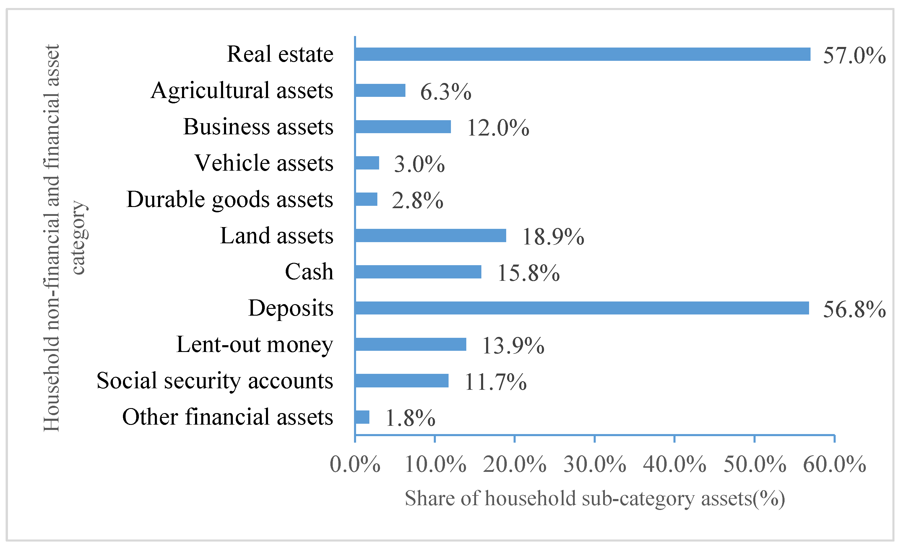
2. Evolution and Characteristics of China’s Farmland Rental Market and Household Assets

The emergence and development of the farmland market in China is driven by rural land system reform. Since 1978, a ‘household responsibility system’ has had an influential effect, marking the outset of de-collectivization of agricultural production in China. Few households were engaged in farmland rental activities in the late 1980s and early 1990s due to the existing rural land system [27,28]. The emergence of a farmland rental market in China followed when the 15-year contractual period was extended to 30 years in 1998 [5,29], and farmland rental activities subsequently expanded rapidly. According to a nationwide study by the China National Statistical Bureau in 2001, 9.5% of households rent farmland. The Rural Land Contracting Law, initiated in 2003, defines land tenure rights as property rights and explicitly prohibits land redistribution of any form by village officials during the 30-year term of the land contract granted to all farmers [29]. Chaotic land reallocations due to demographic changes, land expropriation, and forced land transfers without proper economic compensations are detrimental to farmers’ legitimate land tenure rights and the development of farmland rental markets in rural China [30]. As of 2003, farmers were entitled to transfer farmland use rights, leading to an increase in farmland rental activities and, in return, the provision of more flexibility in farmland allocation in China. Adjustment to farmland tenure rights also affects the labor allocation of rural households and, more generally, their engagement in off-farm activities. This has made it possible to lease farmland and enhance the supply of farmland, accelerating the development of the farmland rental market. Since the initiation of the Rural Land Contracting Law reform in 2003, a series of policy changes have been introduced, among which the 2009 land reform featuring farmland certification and more flexible farmland rental has been the most influential change. The land certification program in China aims to better secure land tenure rights and further strengthen households’ perception of land tenure security, making the circulation of land use rights more flexible by allowing farmers to customize the leasing period with another party in the same local rental market. A household survey in six piloted provinces shows that this has contributed to a 3.9% increase in the proportion of farmland leasing [31].
After the farmland certification initiative, the opaque ‘farmland use rights’ were separated into two distinct entities: operation rights and the contract rights. This officially acknowledged farmers’ rights to lease out an operation while preserving the contract rights and profiting from subleasing farmland for the first time. Rural households can earn both farmland rental income and earnings from off-farm employment with an institutional design that aims to remove previous constraints on access to the farmland rental market. This encourages both kinds of farmland rental activities—leasing of farmland and tenancy of farmland. At the same time, some farmers are not affected by the land reform and still operate their own farmland (i.e., being autarkic in the rental market). The aggregate effect of the 2009 land reform on rental market participation is shown to be positive. A significantly higher participation rate in the farmland rental market has been witnessed following the land tenure reform and, as Figure 1 shows, farmland transfer activities were more active in the period 2007–2017, and the transfer ratio of cultivated land in China reached its peak in 2017, 37%. Initially the pace of development was relatively slow, accompanied by the reform of China’s rural land system as shown in Figure 1. By 2020, according to the Statistical Annual Report on China’s Rural Policy and Reform, 36% of cultivated land had entered in the land rental market1, the total size of which amounts to 565 million mu (approximately 37.64 million ha).
Chinese households’ wealth consists of six forms of assets, namely financial assets, real estate, movable properties and durable goods, productive and operational assets, and land. Chinese household assets demonstrate the following features: a large proportion of real estate, a single category of financial assets holdings, and a significant difference between urban and rural areas (China Household Wealth Survey Report, 2019). In China, 93.03% of households own one house, and the net real estate value of urban households accounted for 71.35% of household wealth, while rural households accounted for only 52.28%. The proportion of financial assets and non-financial assets in rural household total wealth were 7.0% and 93.0% in 2013, respectively (Report on the Development of Household Finance in Rural China, 2014). Moreover, land and housing assets made up the largest proportions of non-financial assets, accounting for 57.0% and 18.9%, respectively, while vehicle and durable goods assets accounted for the smallest, 3.0% and 2.8%, respectively, as shown in Figure 2. Agricultural and business assets accounted for 6.3% and 12.0%, respectively.
In addition, the financial assets of China’s households are mainly in form of cash and deposits, accounting for nearly 90% of household financial assets (China Household Wealth Survey Report, 2019). Compared with urban households, rural households have a higher proportion of cash in hand, current deposits and fixed deposits, and rural households’ financial assets are more concentrated in low-risk and low-return deposits. As shown in Figure 2, cash and deposits were the largest proportions of financial assets, accounting for 15.8% and 56.8% respectively, followed by lent-out money and social security accounts, accounting for 13.9% and 11.7% respectively, while other financial assets such as stocks and funds accounted for the smallest, 1.8%. Further, the aggregate household participation rate in the stock market is only 8.8%, with urban households and rural households accounting for 16.6% and 1.9%, respectively, showing the limited participation of rural households in financial risk markets [26].
With the development of the farmland rental market, rural households can earn both farmland rental income and wages from off-farm employment by having access to the farmland rental market, which encourages both kinds of farmland rental activities—leasing and tenancy of land.2 Household asset allocation behavior may adjust with changes in agricultural production driven by farmland rental activities, making household access to the farmland rental market display different asset allocation characteristics.

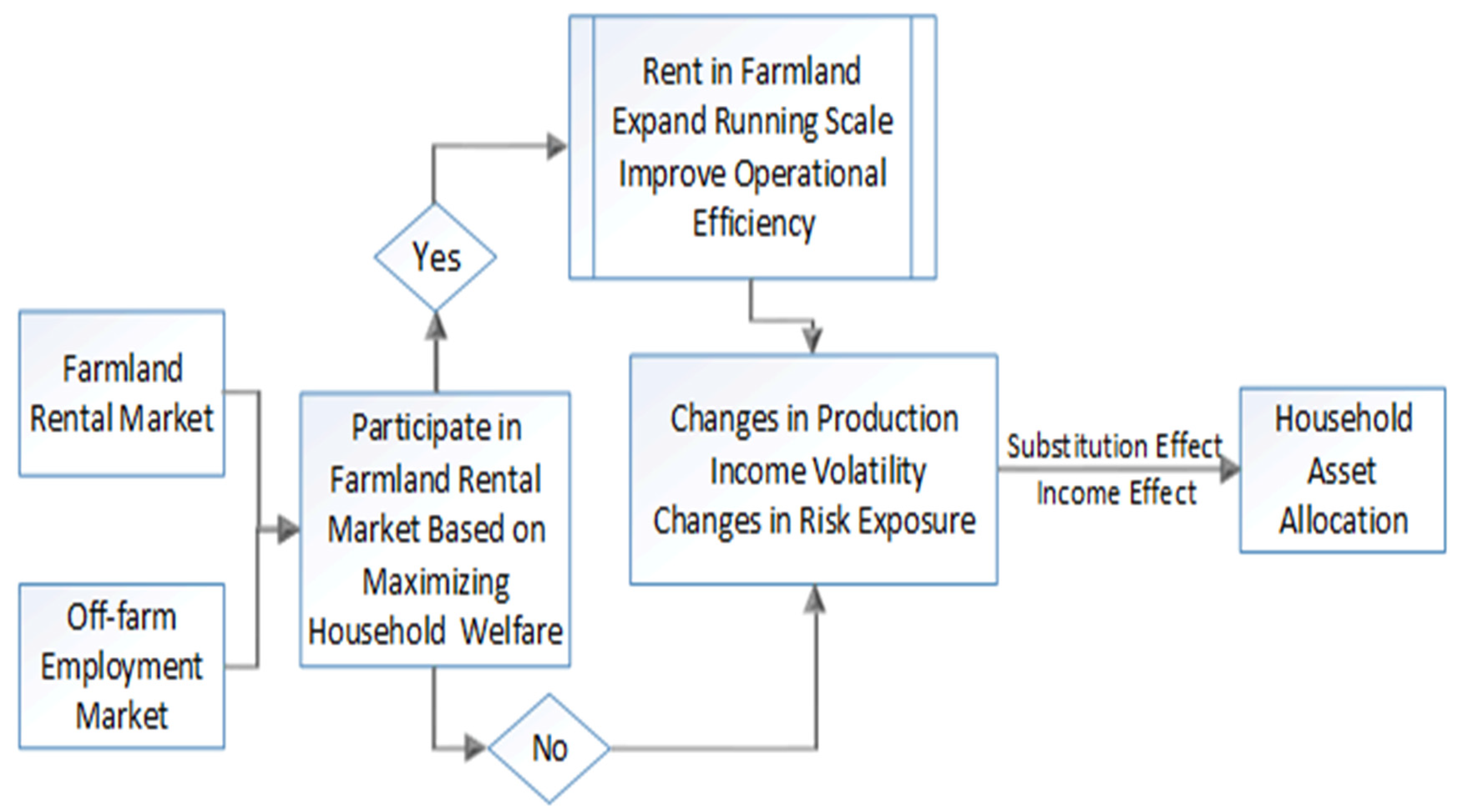
3. Theoretical Analysis

The development of the farmland rental market has helped realize the flexibility of farmland factor allocation, heralding a moderate scale of agricultural production and deepening the professional division of labor [32,33,34]. Changes in agricultural production modes are essentially alterations in the allocation of human capital and financial capital related to land allocation [9,28,35,36,37]. Households make decisions on whether to participate in the farmland rental market and how to participate based on their endowments, such as labor, capital, land and skill [8,9,34,38], to pursue the achievement of Pareto improvement in household welfare, which causes the household adjust resource allocation for higher efficiency to respond [28,39,40,41]. Research shows that households adjust their portfolio holdings when switching jobs, motivated by hedging risk due to income volatility [11,12,19,42,43]. On the one hand, participation in the farmland rental market has helped achieve Pareto improvement in welfare, resulting in relaxed budget constraints on consumption and investment for households and directly affecting households’ asset selection behavior. This is referred to as the income effects of farmland rental market participation on household asset allocation. On the other hand, participation in the farmland rental market directly determines changes in household production activities and labor employment, inducing investment behaviors to alter. This is referred to as the direct substitution investment effect of farmland rental market participation on household asset allocation. Risk exposure of households has also changed with the land rental market participation, impacting asset choice behavior based on the demand for precautionary savings, liquidity needs, and risk allocation [44]; that is, there has been an indirect substitution effect of farmland rental market participation on household asset selection.

3.1. The Income Effect of Farmland Tenancy on Household Asset Allocation

Theoretically, tenancy farmland aims to improve the efficiency of resource allocation for households to participate in the farmland market and change the resource allocation to achieve Pareto improvement in welfare, without which households would not be motivated to participate. In other words, only when the returns from farmland rental participation from agricultural production is equal to or exceeds the sum of the opportunity cost of off-farm employment and farmland rent income will households participate in the farmland rental market and rent in farmland [8].
The income of the farmland tenancy household participants is given as
π 1 = W n f a r m L n f a r m + ( L a n d o w n + L a n d i n ) ( P Y c r o p C l W f a r m ) L a n d i n r l a n d
where W n f a r m and L n f a r m are the returns of off-farm employment and the number of laborers in off-farm employment respectively, and L a n d o w n and   L a n d i n are the amounts of farmland owned by households and rented from others respectively. We assumed that households grew only one crop in the agricultural production under which the crop output per unit of land is Y c r o p , and the crop’s market price is P . The labor needs per unit of land are l , and the cost of other materials needed per unit of land is C , except for labor. W f a r m is the average wage of agricultural labor employed in the village; r l a n d is the rental price of a unit of farmland.
The labor endowment of households is given as
L t o t a l = L f a r m + L n f a r m  
( Land own + Land in ) l = L farm + L emp
where L f a r m and L n f a r m     are the numbers of agricultural labor and off-farm employment labor in households, respectively. The household makes the optimal labor allocation decisions between agriculture and off-farm for the whole household’s benefit under the constraint of labor endowment in Equation (2).
The labor required for agricultural production is from labor endowment owned by households or hired labor from the labor market at the price of W f a r m , as shown in Equation (3). The amount of hired labor from the labor market is L e m p .
Bringing Equation (2) and Equation (3) into Equation (1), and taking the derivative for L a n d i n , under the first-order condition, π 1 / L a n d i n = 0 , the equilibrium is given as
P Y c r o p C l W f a r m r l a n d = l W n f a r m
At this time, the household has achieved income maximization. It can be drawn from Equation (4) that when the net agricultural income (total revenue minus total cost) per unit of farmland is equal to the off-farm employment wage of the labor required to be invested in the unit of farmland, the farmland tenancy-in for households reaches equilibrium.
Households participating in the farmland rental market can achieve welfare improvements such as increased income and poverty reduction [29,45,46,47,48,49], owing to the adjustment of allocation of resources, such as human capital, land, and capital. Income is closely related to the budget constraint boundary of household saving, consumption, and investment. Changes in household income can lead to an alteration in saving, consumption, and investment behavior, under which asset choice behavior also alters. An increase in income helps raise the marginal propensity to consume and promotes household participation in the allocation of risky assets [13,16,21,25,43]. Furthermore, income volatility resulting from agriculture production issues with weather and market risks after the tenancy of farmland will also increase households’ willingness to save and reduce the households’ allocation to risky assets [12,15,18,19,42,50,51].
According to classical asset selection theory, the utility of households U ( C t ) is given as
U ( C t ) = ( 1 γ ) · e x p ( γ C t )
where γ is risk aversion, and the consumption in period t is C t . The household pursues the utility maximization in the whole life cycle T , shown as
MAX [ E ( t = 0 T 1 ( 1 + θ ) t U ( C t ) ) ]
where θ is the discount factor, and the expected value of households is E ( · ) . t represents different periods. The asset allocation behavior of households is subject to the following constraints
A t + 1 = ( A t + I t C t ) [ ( 1 + r p ) w + ( 1 + r f ) ( 1 w ) ]
where A t and A t + 1 are the wealth of the households in periods t and t + 1 , respectively, and household income in period t is I t . w is the proportion of wealth invested in risk-free assets. r p and r f are the return of the risky asset and safe assets, respectively, assuming that there is only one kind of risky asset and safe asset. Household income changes from I t to I t + I t after participating in the land rental market. I t is the change of household income due to adjustment of resource allocation. Therefore, the constraints of asset choice faced by households participating in the farmland rental market, participants, are given as
A t + 1 = ( A t + I t + I t C t ) [ ( 1 + r p ) w + ( 1 + r f ) ( 1 w ) ]
In this case, households adjust their saving and investing behavior following the constraints’ change, constituting an income effect of farmland tenancy on household asset allocation.

3.2. The Substitution Effect of the Tenancy of Farmland on Household Asset Allocation

Participation in the farmland rental market results in an alteration to the running scale through the farmland tenancy, not only elevating the efficiency of existing agricultural machines and equipment but also incentivising households to increase extra investment in agriculture [28,39,48,52,53] to control per hectare machinery services expenditure and timeline costs based on seasonal characteristics of agricultural production. Whether to rent farmland makes asset choice behavior different between tenants and autarkic farmers not participating in the farmland rental market, referred to as the direct substitution effect of farmland tenancy on household asset allocation.
In addition, risk exposure also changes with a switch to production behavior and income owing to whether to enter the farmland rental market and rent farmland. Generally, households will work more, save more, and adjust their portfolio to cope with any risk exposure caused by income volatility and variation in background risk [11,12,54]. There are three types of precautionary motives directly relevant to an agent’s demand for holding assets: the precautionary saving motive, the desire to moderate total risk exposure, and the precautionary demand for liquidity [44]. These play an essential role in the impact of farmland tenancy on household asset allocation. On one hand, increased volatility in income growth caused by the tenancy of farmland will increase households’ background risk exposure, leading to an increase in households’ demand for precautionary savings and liquid assets, subsequently crowding out the allocation of other assets to keep households’ risk levels manageable. On the other hand, there is also an incentive to simultaneously hedge income risk in asset allocation for farmland tenants, eliminating the insurable part of income risk by holding some risky assets to reduce the impact of uncertainty on household consumption and wealth. Generally, farmland rental households will face more significant industrial and natural risks as the scale of production expands, leading to an increase in household background risk due to constant macroeconomic fluctuations. The impact of these changes in risk exposure on household asset allocation owing to the tenancy of farmland is the indirect substitution effect of the farmland tenancy on household asset allocation.
In summary, the mechanism affecting farmland rental market participating households’ asset allocation in this paper is shown in Figure 3. Based on the analysis above, the model yields the following predictions.
Hypothesis 1 (H1):
The tenancy of farmland affects household asset allocation through income effect derived from welfare improvements.
Hypothesis 2 (H2):
The tenancy of farmland affects household asset allocation through direct substitution effect of farmland rental market participation.
Hypothesis 3 (H3):
The tenancy of farmland affects household asset allocation through indirect substitution effect of farmland rental market participation.

4. Methodology and Data

4.1. Methodology

Whether a household participates in the farmland rental market is an obvious ‘self-selection’ behavior. Based on Rubin’s causal inference theory, we employed the propensity score matching with a difference-in-difference" (PSM-DID) approach to evaluate the effect of the tenancy of farmland on household asset allocation on the consideration that selection bias and the endogeneity of observable and unobservable confounding factors may affect the results, such as personal preference and cognitive discrimination which may or may not vary over time.
The key to PSM-DID is to look for non-participants for each participant with similar characteristics except for participation in the land rental market. In this paper, we employ a binary logit model to calculate propensity scores for the tenancy of farmland when controlling the characteristics of the head and the whole household, macroeconomics, and factor markets in the region. The logit model for estimating propensity score matching is given as
P r o i t = β 0 + β 1 h e a d i , t 1 + β 2 h o u s e i , t 1 + β 3 e n v i r i , t 1 + ε i
where P r o i t is the probability of participating in the farmland rental market and the tenancy of farmland for household i in period t . The vectors h e a d i , t 1 and h o u s e i , t 1 are the head characteristics and the whole household characteristics for household i in period t 1 , respectively. e n v i r i , t 1 is the vector of macroeconomics and factor markets where household i is located in period t 1 . ε i is the random error. β 0 ,   β 1 , β 2 and β 3 are parameters to be estimated.
The effect of the farmland tenancy on household asset allocation employing PSM-DID, A T T , is given as
A T T = 1 N 1 i : D i = 1 [ ( Y i t Y i t 1 ) j : D j = 1 w ( i , j ) ( Y j t Y j t 1 ) ]
where D i indicates whether a household i has rented farmland, 1 represents the participant participating in the farmland rental market and the tenancy of farmland; 0 otherwise. N 1 represents the number of participants. Y i t and Y i t 1 are the household asset allocation variables for the household i in the period t and t 1 , respectively. w ( i , j ) is the corresponding weight of a matched pair, ( i , j ) , that a participant matches with a non-participant when controlling the variables affecting the decision to enter the farmland rental market.

4.2. Data Source

The data in this research comes from the two annual surveys of the China Household Finance Survey (CHFS) conducted in 2013 and 2015 and considers the rapid evolution of China’s farmland rental market during the period between 2007 and 2017. CHFS samples are distributed in 29 provinces in China and conducted every two years, represented at the national and regional levels in our research. We imposed several restrictions for households included in our analysis. First, we selected only households in both years of the survey in rural areas, deleting households in urban areas. Second, due to the separation of ownership that belongs to the collective or state, the contractual rights, and the management rights of farmland in China’s current land system, the households involved in the farmland rental market included two types: one was households that did not have the contractual right but could rent farmland to carry out agricultural production; the other was households that enjoyed the contractual right of land, meaning the household could lease out or rent in farmland or not even participate in the farmland rental market and only carry out self-sufficient agricultural production on their own contracted farmland. Only the latter was considered in our research sample to control for household heterogeneity as far as possible. Third, the samples used for analysis only retained households possessing the contractual right of farmland in rural areas that neither participated in the farmland rental market nor rented farmland in 2013. This provided a two-period balanced panel data representing 3650 households. In our analysis, the households that did not participate in the farmland rental market in 2013 but participated in the tenancy of farmland in 2015 were regarded as participants, accounting for 12% of the cohort analyzed. Simultaneously, households that did not participate in the farmland rental market in 2013 and 2015 were the control group in our analysis.

4.3. Variables Description

4.3.1. Dependent Variable

The dependent variable this research focused on was household asset allocation, which involved two dimensions: (1) whether a household participated in investment for a specific category of assets; and (2) the participation depth of households investing in that category of assets [14,18]. The former was represented by creating a dummy, 1 representing if a household had participated in the investment of a category of assets, otherwise shown to be 0. The latter was measured by the amount or proportion of household holdings for a certain category of assets [11,15,18,55,56].
This study followed the conventional categorizations of assets used in the literature. The total assets comprised two components—financial and non-financial assets [56]. The non-financial assets referred to current values of real estate (ownership of home residence, special agricultural equipment, vehicle and consumer durables, and other properties) and business assets (ownership of business, professional practices). For the financial assets we adopted a three-way classification scheme which included safe assets (checking and saving accounts, government saving bonds3), risky assets4 (stock, money market funds, mutual funds, and private loans to other households) and social security accounts (pension and annuity funds, medical insurance, and housing funds). In addition to the amounts of various assets we further explored the tenancy of farmland on (1) the accumulation of household wealth, (2) the amount of non-financial assets and subcategory assets within non-financial assets, (3) the share of financial assets within assets, (4) the share of risky assets and safe assets within financial assets respectively, and (5) the incidence of risky asset holdings. The definition and description of households’ various assets are shown in Table 1.

4.3.2. Core Explanatory Variable

In general, participants’ behavior in the farmland rental market involves two types: their tenancy of farmland from other households and the leasing of their own contractual land. This study does not cover both kinds of market behaviors, focusing only on the effect of farmland tenancy behavior specifically. Therefore, participation in the farmland rental market and the tenancy of farmland was measured by creating a dummy, 1 for participants as tenants and 0 for otherwise. In the benchmarking, intensity in the tenancy of farmland was not considered, and the heterogeneity between households with different intensities in the tenancy of farmland was ignored. To this end, we divided the participants, tenants, into two groups by the average area of rented farmland—a low intensity group and a large intensity group—to further explore the heterogeneous influence of farmland tenancy on household asset allocation.

4.3.3. Control Variables

There are many factors that can affect household asset allocation behavior besides farmland rental activities, such as household head, household characteristics, and factor market. Some variables were controlled in this article by referring to the conventional literature [11,13,29,38,45,46,56,57].
First, the demographic characteristics of the household including age, gender, marriage, education, and health status will affect the choice and allocation of household assets [13,14,18,58]. We used age, gender, marriage, and education of the household head to identify demographics. In order to better describe the possible nonlinear effect of age on the results, the age of the head was measured by a series of dummies, seen in Table 1.
Second, the overall economic characteristics of the household, such as risk aversion, financial literacy, household wealth and income, and background risk, are closely related to its consumption and investment behavior [11,13,14,15,16,18,19,42]. Therefore, we also controlled those confounding factors in our analysis as far as possible. Apart from this, household endowment such as labor and land and off-farm employment opportunities not only directly affect whether a household participates in the farmland rental market but also indirectly affects agricultural investment [28,40,45,59,60,61]. We used the value of owned contractual right farmland, the number of laborers, whether to run a business, and the per capita non-agricultural income to represent the endowment characteristics and off-farm employment opportunities of households, respectively. In addition, the quadratic term of household wealth was put into the model to capture the possible nonlinear effects of wealth on the results [18]. The detailed definitions of the variables are shown in Table 1.
Finally, household asset allocation behavior, as an economic behavior, is also changed following macroeconomic changes via the variation of economic expectations, budget constraints and background risks such as policies, finance, institutions, and factor market [12,20,22,23,25,62]. In this study, urban per capita wages and the area’s incidence of land circulation represented factor market characteristics. The detailed definitions of variables are shown in Table 1.

5. Results and Discussion

5.1. Descriptive Statistics of the Research Variables

Among all the tenants, the average area of farmland rented by households was 9.98 mu5, and the standard deviation was 24.30 mu, indicating that the intensity of participating in the farmland rental market varied significantly among participants. Moreover, 329 households rented in farmland less than the average area of farmland tenancy, accounting for 76.7% of all the treated group households.
Table 1 and Table 2 show the descriptive statistics of household assets in the study. For the overall households, all non-financial assets holdings and total assets increased in 2015, compared with those in 2013. However, the share of financial assets in 2015 decreased. In addition, the incidence of risk asset holdings, share of risky assets and safe assets increased in 2015, compared with those in 2013.
From the perspective of the treated group (tenants), the household total assets were CNY 230,761 (23.0761) and CNY 291,664 (29.1664) between ex-ante and ex-post. Relatively, they were CNY 253,474 and CNY 261,899 for non-tenants, respectively. The change of total assets was significantly distinguished between tenants and non-tenants at a level of p < 0.01, demonstrating that the total assets of farmland tenancy households increases more than those of non-tenants. In terms of the non-financial assets, they all increased after renting farmland, and the changes between tenants and non-tenants differed significantly at a level of p < 0.05, indicating that the farmland tenancy made households increase investment in non-financial assets and obviously influenced the adjustment of the structure of non-financial asset holdings. Specifically, the tenants increased their holdings of agricultural assets, vehicle assets, durable goods assets, housing assets, and business and other non-financial assets compared with non-tenants, among which the largest increase was in housing assets and the smallest increase was in durable goods assets. As for financial assets, the proportions of financial assets in total assets were 13.20% and 9.93% between ex-ante and ex-post for tenants, and they were 12.65% and 9.05% for non-tenants, respectively. There was no difference in change in share of financial assets in total assets. However, the share of risky assets in financial assets were 3.86% and 6.23% before and after the farmland tenancy for tenants, and the change was significantly greater than that of non-tenants at a level of p <0.05, which illustrates that farmland tenancy may have influenced the adjustment of financial assets allocation. In addition, there was no significant change in the share of safe financial assets holdings and incidences of risky assets between the tenants and non-tenants.
Through the statistical analysis it can be found that there was a significant difference in changes to household asset allocation behavior between the tenants and non-tenants. Whether the difference in adjustment of asset allocation was due to the behavior of household participation in the farmland rental market requires further verification and examination with a causal inference approach.

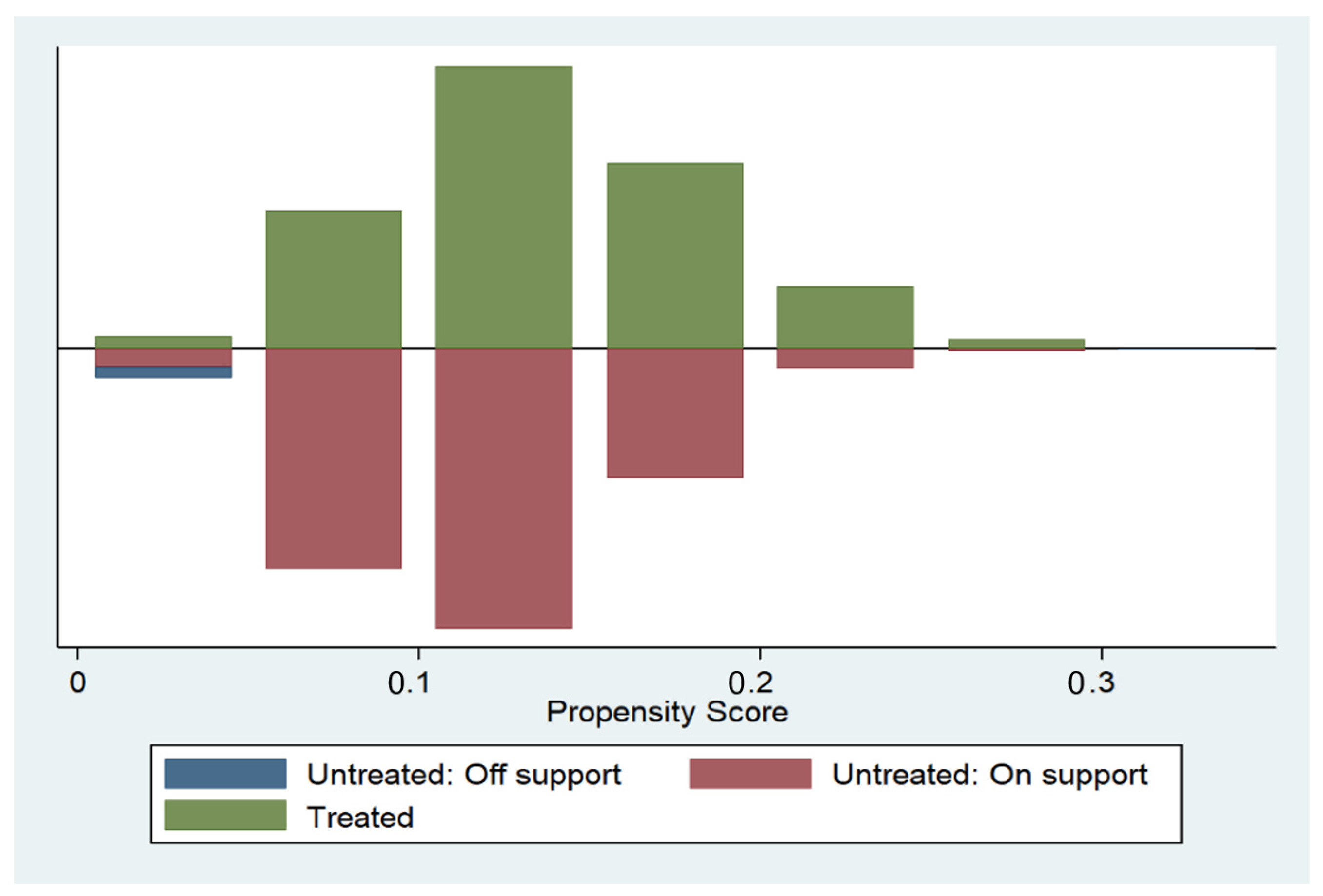
5.2. Propensity Score Matching Procedure

Table 3 shows the result of the logit model of factors that affect tenancy of farmland decisions with Equation (9). The following features about households’ farmland tenancy behavior have been presented.
First, age and education levels were critical factors affecting farmland tenancy decisions made by households. In general, younger laborers had more agricultural and off-farm employment opportunities, resulting in the flow of farming laborers into non-agricultural industries. However, as age increased, the non-agricultural employment opportunities rural laborers had also decreased and the possibility of engaging in agricultural production increased simultaneously. Since agricultural production is a labor-intensive industry, older laborers were also less likely to engage in agricultural production. As shown in Table 3, households whose heads were above the age of 60 restrained themselves from the tenancy of farmland significantly at p < 0.05, which is consistent with the current agricultural production reality in China. Further, households that attained higher education levels showed significantly less will to rent farmland at p < 0.05, with more opportunities to choose between agriculture and off-farm employment available. These findings are consistent with prior research on China’s land market participation [38,41,45,46,63].
Second, there was path dependence in the choice of production and operation modes for households. As shown in Table 3, households whose heads had been engaged in farming were significantly more likely to rent farmland in comparison with households whose heads had not farmed at p < 0.01 , indicating that path dependency in the choice of production and operation modes for households existed. In addition, the labor-intensive nature of agriculture also determined that households with large labor endowments tended to rent farmland significantly at p < 0.1 , which is also consistent with previous research [38,41,46,63].
Third, there was a significant ‘herd effect’ in household’s decision-making regarding participation in the farmland rental market and the tenancy of farmland at p < 0.05 . On the one hand, the incidence of farmland tenancy in the area where households were located contributed to the development of the farmland rental market, which is convenient for the households with participation willingness. On the other hand, the decisions to enter the farmland rental market were influenced by other households having entered the market via conformity, which can be indicated from the coefficients of the tenancy-in rate in Table 3, consistent with the results of Yan and Huo (2016).
Off-farm employment opportunities embedded in the macroeconomic environment were key factors for household participation in the tenancy of farmland, although not significant in our results statistically. The adjustment of the allocation of farmland resources was accompanied by changes in the rural labor force in China. Off-farm employment opportunities and increased non-agricultural wages were the fundamental reasons for households to participate in farmland rental activities [28,38,41,45,64]. Previous research illustrates that households with high off-farm employment opportunities and abilities, measured by non-farm income, are less likely to enter the farmland market and rent in farmland [38,41,45,64].
The PSM-DID approach works on the condition that the basic premises of overlap assumption and the conditional parallel trend hypothesis are satisfied. For the PSM-DID approach with two-period panel data, the conditional parallel trend hypothesis means that it is necessary to ensure the same distribution of covariates used for propensity score matching between the treated group and the control group before treatment, which is called the data balancing test.
The overlap assumption, called the matching assumption, is that there must be considerable overlap in the propensity score between treated and control groups. Figure 4 shows the result of the common hypothesis test using a kernel function to match treated group individuals with control group individuals. The propensity score employing the logit model Equation (9) is overlapped between the treated group and control group, indicating that there is only a tiny sample lost when performing propensity score matching. This suggests that the sample matching quality is sound and the common support hypothesis has been satisfied.
Table 4 shows the results of the data balancing test. After matching, the pseudo becomes lower, and the LR statistic of the model for the joint significance test of the covariates is not significant compared to the ex-ante. Meanwhile, the standardized bias of covariates used for the propensity score matching is reduced to less than 10%, and the mean bias is also lower than 20% after matching. Further, most t-tests of covariates of both the participants and non-participants do not reject the null hypothesis that there is no significant difference in both after matching, indicating that there is only a systematic difference in the distribution of covariates after matching, suggesting that the bias caused by sample self-selection between the treatment group and the control group is effectively eliminated by using the matching approach. That is, after matching, the covariates of the treated group and the control group have the same distribution. The slight differences between the two groups are based only on the different performances of an individual. There is no systematic difference between the two groups statistically, meaning the treated group and control group samples are considered to be from the same sample before treatment; thus, the balanced hypothesis is also satisfied [65,66,67,68]. The balanced hypothesis being satisfied ensures that the counterfactuals constructed in this study are reasonable.

5.3. The Impacts of Farmland Tenancy on Household Asset Allocation

Different matching methods were used to ensure the robustness of research results. All results in Table 5 were obtained using bootstrap sampling of 500 replications. Among them, columns 2–3 indicate the results of adopting PSM-DID with kernel regression matching, and columns 4–5 show the results of adopting PSM-DID with local linear regression matching. Table 5 presents the effects of participation in the land rental market on household wealth and asset allocation.
From the aspect of household wealth, there is no significant difference in the change of total assets (row 3) between tenants and non-tenants, indicating that the farmland tenancy had no impact on household accumulation of wealth. A similar result is obtained from row 10, showing that the farmland tenancy had no significant impact on the structure of household wealth holdings, and that farmland tenancy has not led to the adjustment of the structure of household wealth holdings.
From the perspective of household asset allocation, there are obvious differences between asset allocation behavior of tenants and non-tenants. Specifically, there is a significant difference in the change of durable goods assets (row 7) between tenants and non-tenants at a level of p < 0.05 , suggesting that the increase in durable goods assets was greater for tenants compared to non-tenants. The tenants increased about CNY 11406 more in durable goods asset investment than non-tenants from our empirical results, thus improving family welfare. The effect of the tenancy of farmland on durable goods assets is similar to that of prior research findings [69]. The increase in durable goods assets for farmland tenants may result from the investment in televisions, mobile phones, and computers that would help households acquire agricultural production information or technology. Regarding the agricultural assets, those of tenants increased CNY 10507 more than those of non-tenants (row 5), but this is not significant, providing no statistical evidence of investment incentives in agricultural machinery for the tenancy of farmland.
In addition, housing assets allocation (row 8) shows a similar change between tenants and non-tenants at a level of p < 0.1 , demonstrating that tenants gained about CNY 21,9918 in housing assets than non-tenants from our empirical results. There are two main reasons for the increase in housing assets: one is increased investment in housing assets, and the other is the appreciation of houses derived from the development of the real estate market. The former mostly involves the purchase, decoration, reconstruction, and expansion of houses. The mean number of houses owned by rural households in 2013 was 1.07 and was 1.60 in 2015. Both t-test and PSM-DID analysis showed that there were no statistical differences in the number of houses ( d i f f = 0.1463 , S . E . = 0.4248 , p = 0.7306 > 0.1 ) and in the change of the number of houses ( n u m h o u s e = 0.3790 , S . E . = 0.3416 )9 between tenants and non-tenants, which can suggest that the increase in household housing assets was not caused by the purchase of houses. Does the difference between the changes in housing assets between tenants and non-tenants stem from the diversity in housing decoration, expansion, or reconstruction of houses? Therefore, we further examined the expenditure on housing assets, and found that the change in expenditure on decoration, reconstruction, and expansion of the households was not significantly different between tenants and non-tenants ( e x p e n d h o u s e = 0.1201 , S . E . = 0.1354 ), which helped us deduce that the increase in household housing assets was also not caused by the investment in housing, such as decoration, reconstruction, and expansions of houses. In addition, we also examined the changes in the value of commercial real estate alone, and find a significant difference between tenants and non-tenants ( h o u s i n g c o m m e r c i a l = 0.0709 , S . E . = 0.0646 ). All the above analysis gives us reasons to doubt the difference in changes in housing assets between tenants and non-tenants may be caused by the imbalance of the appreciation of housing assets derived from the rapid development of the real estate market, rather than the adjustment of household asset allocation due to farmland tenancy.
Nevertheless, there was no significant difference in the change of other subcategory non-financial assets (row 6 and row 9) between tenants and non-tenants. In terms of the structure of household financial assets holdings, there was also no significant difference in the share of both risky and safe assets holdings (rows 12–13) between tenants and non-tenants, indicating that farmland tenancy had no impact on the adjustment of the structure of household financial assets holdings. Moreover, the tenancy of farmland had no significant impact on the incidence of risky asset holdings (row 11).

5.4. The Impacts on Household Asset Allocation with Different Tenancy Intensities in the Farmland Rental Market

Table 6 shows the heterogeneous influence of the farmland tenancy on household asset allocation from the tenancy intensities in the farmland rental market. We see a significantly heterogeneous influence on wealth and asset allocation among tenants with different intensities in the farmland rental market. The tenants with large intensity in the farmland rental market have been strongly affected compared to tenants with low intensity in the farmland rental market. The tenancy of farmland with large intensity has not only resulted in positive household wealth accumulation (row 4), but has also significantly increased the investment in agricultural assets (row 6), compared with the tenants with low intensity, providing evidence of investment incentives for the tenancy of farmland. There may be a scale threshold for investment incentives of farmland tenancy in agricultural machinery, which is also in line with our theoretical analysis intuition that the cost of machinery owned by households on unit land will decrease with the increase of rental farmland, compared with outsourced machinery services. Simultaneously, the tenants with large intensity in the farmland rental market had more total non-financial assets (row 5) compared with tenants with low intensity. Moreover, the farmland tenancy also has improved the incidence of risky asset holdings (row 12) and the share of risky assets in financial assets (row 13), ultimately adjusting the structure of financial assets holdings. These findings are consistent with previous research [11,19,43].

5.5. Mechanisms for Farmland Tenancy Affecting Renting-In Household Asset Allocation

We elaborated on how the tenancy of farmland influences household asset allocation in Section 2. The mechanism that the tenancy of farmland works on household asset allocation through the direct substitution effect has been discovered based on the empirical analysis above. H2a has been confirmed. More examination is required to explore if the tenancy of farmland influences household asset allocation through the indirect substitution effect and income effect.
Table 7 displays the change in household income and liabilities between tenants and non-tenants, derived from analysis employing the PSM-DID approach. There was no significant difference in household income changes between tenants and non-tenants, which still stands from the perspective of different intensities in the tenancy of farmland. The results in Table 7 are not consistent with H1. The impacts of the tenancy of farmland on the change to household incomes indicate that the tenancy of farmland has not impacted household asset allocation through the income effect. In addition, we inquired as to whether the household was in debt, and the scale of any household debts, to assess the changes in risk exposure after tenancy farmland indirectly. The data show that the incidence of tenants in debt and the scale of household debt owing to agricultural production increased significantly after tenancy of agricultural land: 2.92% and CNY 3297 more than those of non-tenants, respectively. Further, as shown in Table 7, the debt scale of tenants owing to agricultural production increased significantly at a level of p < 0.01 after tenancy of agricultural land, although the increase in incidence of tenants in debt owing to agricultural production was not statistically significant. This is consistent with previous research [70]. It is interesting that there was no significant difference in the change of the overall household liabilities level between the tenants and non-tenants. We argue that the expansion of production scale resulting from the renting of farmland has changed the risk exposure of households and the demand for preventive savings and hedging risk motive, thus affecting household asset allocation through risk rebalancing. H3 has also been confirmed.
Overall, the tenancy of farmland has worked on household asset allocation through the substitution effect instead of the income effect.

6. Conclusions and Policy Implications

This study explores the following issues under rural land system reform in China: (1) whether participation in the farmland rental market and the tenancy of farmland affects a household’s asset allocation behavior; (2) what the effect of the tenancy of farmland on household asset allocation is, and (3) how the tenancy of farmland influences household asset allocation. Using a sample of China’s rural households with farmland contract rights we employed propensity score matching with a difference-in-difference approach to explore the impact of the tenancy of farmland on household asset allocation and examine the mechanisms for farmland tenancy affecting household asset allocation. We draw four conclusions from these results. First, there is a ‘herd effect’ in the household decision-making in participation in the farmland rental market and the tenancy of farmland. Second, the tenancy of farmland has caused the adjustment of household asset choice behavior, increasing investment in durable goods assets. Third, there is heterogeneity in the effects on asset allocation among tenants with different intensities in farmland tenancy, presenting relatively more substantial impacts on the change of asset allocation for tenants with high intensity in the farmland rental market. The tenancy of farmland with high intensity has not only boosted tenants’ wealth accumulation but has also increased the investment in agricultural assets and risky asset holdings (both incidence and the share of risky financial assets). Tenancy of farmland does not necessarily bring about the household’s increased investment in agricultural machinery, and only when the area of farmland tenancy reaches a certain scale threshold will households increase their investment in agricultural machinery. Forth, the tenancy of farmland has worked on household asset allocation through the substitution effect instead of the income effect.
In general, even though the agriculture sector is not so profitable compared to the industry sector in China, the wealth effect of farmland holding remains significant. Based on the above conclusions, three policy implications may be put forward: first, there should be encouragement through fiscal and financial policies to rent large-scale farms and for new agricultural operation entities to obtain economy of scale, for family farms, cooperatives, professional large households, and agricultural companies. Second, reducing the cost of agricultural machinery via technological progress or agricultural machinery subsidies can both increase household income and accumulate wealth for tenant households, and ensure food security. Third, improving farmers’ financial literacy and inclusive financial services, such as loan products, deposit products, and fund securities suitable for farm households, will facilitate productive asset investment and interest-bearing asset allocation, thus improving the efficiency of household wealth accumulation.
With the limitation of data used in this study, the empirical analysis for the possible effects on asset allocation in the long term inferred from the practice of successive reforms of China’s rural land system fails, and only the short-term effects of entry in the farmland rental market and the tenancy of farmland on household asset allocation are explored. Further research is needed to assess the long-term impact on household asset choice behavior.

Author Contributions

Conceptualization, L.X. and Y.J.; methodology, L.X.; software, L.X. and J.W.; writing—original draft, L.X. and Y.J.; writing—review and editing, L.X., A.A.C. and Y.J.; supervision, Y.J.; project administration, Y.J. All authors have read and agreed to the published version of the manuscript.

Funding

This study was supported by a key research project of the National Social Science Fund of China, “Research on the Mechanism and Path of Rural Land and Finance Integration under the Background of the ‘Three Rights Division’ Reform” (No.: 20AJY011). We also gratefully acknowledge data supports from Survey and Research Center for China Household Finance.

Institutional Review Board Statement

Not applicable.

Informed Consent Statement

Not applicable.

Data Availability Statement

The data presented in this study are available from the Survey and Research Center for China Household Finance (https://chfs.swufe.edu.cn, accessed on 10 September 2022).

Conflicts of Interest

The authors declare no conflict of interest.

Notes

1
According to land transfer practice in rural China, there are five forms involved in the land transfer, transfer the possession of land, exchange, leasing subcontract, becoming a shareholder and other forms that comply with relevant laws and national policies. Here the transfer of cultivated land covers the above 5 forms and is defined by the Administrative Measures for the Transfer of Rural Land Management Rights before 2021. But the Administrative Measures for the Transfer of Rural Land Management Rights has been revised in 2021, and only leasing subcontract (transfer the possession of land), becoming a shareholder and other forms that comply with relevant laws and national policies are included in the land transfer.
2
From the perspective of the supply and demand of the farmland rental market, the participation of the household’s farmland rental market mainly includes two types: leasing out farmland or tenancy of farmland. The former rent out their farmland management right, while the latter rent in the farmland management rights of others.
3
Because of the social security system in rural China, few households have retirement accounts. Therefore, retirement account assets were not considered in our study.
4
In combining the conventional literature with the practice of asset allocation in rural China the measurement of financial assets and risky assets have been adjusted slightly in our study.
5
1 mu = 667 m2 or 0.067 ha.
6
0.1140 is the arithmetic mean of the results of PSM-DID with KM and PSM-DID with LLRM.
7
0.1050 is the results of PSM-DID with KM.
8
2.1991 is the arithmetic mean of the results of PSM-DID with KM and PSM-DID with LLRM.
9
The results in parentheses are obtained by adopting kernel matching and bootstrap sampling 500 replications, and the results using local linear regression matching and bootstrap sampling 500 replications are still robust. The meaning of e x p e n d h o u s e and h o u s i n g c o m m e r c i a l are the same.

References

  1. Doepke, M.; Schneider, M. Inflation and the Redistribution of Nominal Wealth. J. Politi-Econ. 2006, 114, 1069–1097. [Google Scholar] [CrossRef] [Green Version]
  2. Berloffa, G.; Modena, F. Income shocks, coping strategies, and consumption smoothing: An application to Indonesian data. J. Asian Econ. 2012, 24, 158–171. [Google Scholar] [CrossRef]
  3. Wei, S.-J.; Wu, W.; Zhang, L. Portfolio choices, Asset returns and wealth inequality: Evidence from China. Emerg. Mark. Rev. 2018, 38, 423–437. [Google Scholar] [CrossRef]
  4. You, J. Risk, under-investment in agricultural assets and dynamic asset poverty in rural China. China Econ. Rev. 2014, 29, 27–45. [Google Scholar] [CrossRef]
  5. Zhou, Y.; Li, X.; Liu, Y. Rural land system reforms in China: History, issues, measures and prospects. Land Use Policy 2019, 91, 104330. [Google Scholar] [CrossRef]
  6. Fei, R.; Lin, Z.; Chunga, J. How land transfer affects agricultural land use efficiency: Evidence from China’s agricultural sector. Land Use Policy 2021, 103, 105300. [Google Scholar] [CrossRef]
  7. Lu, X.-H.; Jiang, X.; Gong, M.-Q. How land transfer marketization influence on green total factor productivity from the approach of industrial structure? Evidence from China. Land Use Policy 2020, 95, 104610. [Google Scholar] [CrossRef]
  8. Carter, M.R.; Yao, Y. Local versus Global Separability in Agricultural Household Models: The Factor Price Equalization Effect of Land Transfer Rights. Am. J. Agric. Econ. 2002, 84, 702–715. [Google Scholar] [CrossRef]
  9. Jin, S.; Deininger, K. Land rental markets in the process of rural structural transformation: Productivity and equity impacts from China. J. Comp. Econ. 2009, 37, 629–646. [Google Scholar] [CrossRef] [Green Version]
  10. Daymard, A. Land rental market reforms: Can they increase outmigration from agriculture? Evidence from a quantitative model. World Dev. 2022, 154, 105865. [Google Scholar] [CrossRef]
  11. Betermier, S.; Jansson, T.; Parlour, C.; Walden, J. Hedging labor income risk. J. Financ. Econ. 2012, 105, 622–639. [Google Scholar] [CrossRef] [Green Version]
  12. Chang, Y.; Hong, J.H.; Karabarbounis, M.; Wang, Y.; Zhang, T. Income volatility and portfolio choices. Rev. Econ. Dyn. 2021, 44, 65–90. [Google Scholar] [CrossRef]
  13. Bodie, Z.; Merton, R.C.; Samuelson, W.F. Labor supply flexibility and portfolio choice in a life cycle model. J. Econ. Dyn. Control. 1992, 16, 427–449. [Google Scholar] [CrossRef] [Green Version]
  14. Campbell, J.Y. Household Finance. J. Financ. 2006, 61, 1553–1604. [Google Scholar] [CrossRef] [Green Version]
  15. Cardak, B.; Wilkins, R. The determinants of household risky asset holdings: Australian evidence on background risk and other factors. J. Bank. Financ. 2009, 33, 850–860. [Google Scholar] [CrossRef] [Green Version]
  16. Cocco, J.F. Portfolio Choice in the Presence of Housing. Rev. Financ. Stud. 2004, 18, 535–567. [Google Scholar] [CrossRef]
  17. Guiso, L.; Sodini, P. Chapter 21—Household Finance: An Emerging Field. In Handbook of the Economics of Finance; Constantinides, G.M., Harris, M., Stulz, R.M., Eds.; Elsevier: Amsterdam, The Netherlands, 2013; Volume 2, pp. 1397–1532. [Google Scholar] [CrossRef] [Green Version]
  18. King, M.A.; Leape, J.I. Wealth and portfolio composition: Theory and evidence. J. Public Econ. 1998, 69, 155–193. [Google Scholar] [CrossRef] [Green Version]
  19. Heaton, J.; Lucas, D. Portfolio Choice and Asset Prices: The Importance of Entrepreneurial Risk. J. Financ. 2000, 55, 1163–1198. [Google Scholar] [CrossRef]
  20. Malmendier, U.; Nagel, S. Depression Babies: Do Macroeconomic Experiences Affect Risk Taking? Q. J. Econ. 2011, 126, 373–416. [Google Scholar] [CrossRef]
  21. Rosen, H.S.; Wu, S. Portfolio choice and health status. J. Financ. Econ. 2004, 72, 457–484. [Google Scholar] [CrossRef] [Green Version]
  22. Guiso, L.; Sapienza, P.; Zingales, L. Does Local Financial Development Matter? Q. J. Econ. 2004, 119, 929–969. [Google Scholar] [CrossRef]
  23. Park, J.S.; Suh, D. Uncertainty and household portfolio choice: Evidence from South Korea. Econ. Lett. 2019, 180, 21–24. [Google Scholar] [CrossRef]
  24. Perraudin, W.R.M. Inflation and Portfolio Choice. Staff Pap. -Int. Monet. Fund 1987, 34, 739. [Google Scholar] [CrossRef]
  25. Wang, N. Optimal consumption and asset allocation with unknown income growth. J. Monet. Econ. 2009, 56, 524–534. [Google Scholar] [CrossRef] [Green Version]
  26. Yin, Z.; Wu, Y.; Gan, L. Financial availability, financial market participation and household portfolio choice. Econ. Res. J. 2015, 50, 87–99. [Google Scholar]
  27. Yao, Y. The Development of the Land Lease Market in Rural China. Land Econ. 2000, 76, 252. [Google Scholar] [CrossRef]
  28. Gao, L.; Huang, J.; Rozelle, S. Rental markets for cultivated land and agricultural investments in China. Agric. Econ. 2012, 43, 391–403. [Google Scholar] [CrossRef]
  29. Xu, L.; Du, X. Land certification, rental market participation, and household welfare in rural China. Agric. Econ. 2021, 53, 52–71. [Google Scholar] [CrossRef]
  30. Kung, J.K.S.; Shimokawa, S. Land Reallocations, Passive Land Rental, and the Development of Rental Markets in Rural China; AgEcon Search: Foz do Iguacu, Brazil, 18 August 2012. [Google Scholar] [CrossRef]
  31. Wang, Y.; Li, X.; Li, W.; Tan, M. Land titling program and farmland rental market participation in China: Evidence from pilot provinces. Land Use Policy 2018, 74, 281–290. [Google Scholar] [CrossRef]
  32. Yang, X.; Wang, J.; Wills, I. Economic growth, commercialization, and institutional changes in rural China, 1979–1987. China Econ. Rev. 1992, 3, 1–37. [Google Scholar] [CrossRef]
  33. Huang, Z.; Zhou, J.; Huang, X. Does the transfer of farmland use rights increase farmers’ long-term intention to work in cities? Econ. Transit. Inst. Change 2021, 30, 373–392. [Google Scholar] [CrossRef]
  34. Vranken, L.; Swinnen, J. Land rental markets in transition: Theory and evidence from Hungary. World Dev. 2006, 34, 481–500. [Google Scholar] [CrossRef]
  35. Chang, H.; Dong, X.-Y.; MacPhail, F. Labor Migration and Time Use Patterns of the Left-behind Children and Elderly in Rural China. World Dev. 2011, 39, 2199–2210. [Google Scholar] [CrossRef]
  36. Feng, S.; Heerink, N.; Ruben, R.; Qu, F. Land rental market, off-farm employment and agricultural production in Southeast China: A plot-level case study. China Econ. Rev. 2010, 21, 598–606. [Google Scholar] [CrossRef]
  37. Jin, S.; Jayne, T.S. Land Rental Markets in Kenya: Implications for Efficiency, Equity, Household Income, and Poverty. Land Econ. 2013, 89, 246–271. [Google Scholar] [CrossRef]
  38. Yan, X.; Huo, X. Drivers of household entry and intensity in land rental market in rural China: Evidence from North Henan Province. China Agric. Econ. Rev. 2016, 8, 345–364. [Google Scholar] [CrossRef]
  39. Gao, L.; Sun, D.; Ma, C. The Impact of Farmland Transfers on Agricultural Investment in China: A Perspective of Transaction Cost Economics. China World Econ. 2019, 27, 93–109. [Google Scholar] [CrossRef] [Green Version]
  40. Ji, Y.; Yu, X.; Zhong, F. Machinery investment decision and off-farm employment in rural China. China Econ. Rev. 2012, 23, 71–80. [Google Scholar] [CrossRef] [Green Version]
  41. Qian, L.; Lu, H.; Gao, Q.; Lu, H. Household-owned farm machinery vs. outsourced machinery services: The impact of agricultural mechanization on the land leasing behavior of relatively large-scale farmers in China. Land Use Policy 2022, 115, 106008. [Google Scholar] [CrossRef]
  42. Bielecki, T.R.; Pliska, S.R.; Sherris, M. Risk sensitive asset allocation. J. Econ. Dyn. Control 2000, 24, 1145–1177. [Google Scholar] [CrossRef]
  43. Li, R.; Wang, T.; Zhou, M. Entrepreneurship and household portfolio choice: Evidence from the China Household Finance Survey. J. Empir. Financ. 2020, 60, 1–15. [Google Scholar] [CrossRef]
  44. Kimball, M. Precautionary Motives for Holding Assets; NBER Working Papers; National Bureau of Economic Research, Inc.: Cambridge, MA, USA, 1991; p. 3586. [Google Scholar] [CrossRef]
  45. Fei, C.; Weijuan, Z. Land Transfer Incentive and Welfare Effect Research from Perspective of Farmers’ Behavior. Econ. Res. J. 2015, 50, 163–177. [Google Scholar]
  46. Peng, K.; Yang, C.; Chen, Y. Land transfer in rural China: Incentives, influencing factors and income effects. Appl. Econ. 2020, 52, 5477–5490. [Google Scholar] [CrossRef]
  47. Udimal, T.B.; Liu, E.; Luo, M.; Li, Y. Examining the effect of land transfer on landlords’ income in China: An application of the endogenous switching model. Heliyon 2020, 6, e05071. [Google Scholar] [CrossRef] [PubMed]
  48. Zhonghao, Q.; Xingwen, W. How does the transfer of farmland promote the increase of farmers’ income. Chin. Rural. Econ. 2016, 10, 39–50. [Google Scholar]
  49. Zhang, D.; Wang, W.; Zhou, W.; Zhang, X.; Zuo, J. The effect on poverty alleviation and income increase of rural land consolidation in different models: A China study. Land Use Policy 2020, 99, 104989. [Google Scholar] [CrossRef]
  50. Guiso, L.; Jappelli, T.; Terlizzese, D. Income Risk, Borrowing Constraints, and Portfolio Choice. Am. Econ. Rev. 1996, 86, 158–172. Available online: http://www.jstor.org/stable/2118260 (accessed on 11 September 2022).
  51. Xingqiang, H.; Wei, S.; Kaiguo, Z. Background Risk and Investors’ Participation in Risky Financial Assets. Econ. Res. J. 2009, 44, 119–130. [Google Scholar]
  52. Cong, S. The Impact of Agricultural Land Rights Policy on the Pure Technical Efficiency of Farmers’ Agricultural Production: Evidence from the Largest Wheat Planting Environment in China. J. Environ. Public Health 2022, 2022, 3487014. [Google Scholar] [CrossRef]
  53. Najafi, B.; Dastgerduei, S.T. Optimization of Machinery Use on Farms with Emphasis on Timeliness Costs. J. Agric. Sci. Technol. 2015, 17, 533–541. [Google Scholar] [CrossRef]
  54. Aiyagari, S.R. Uninsured Idiosyncratic Risk and Aggregate Saving. Q. J. Econ. 1994, 109, 659–684. [Google Scholar] [CrossRef] [Green Version]
  55. Berkowitz, M.K.; Qiu, J. A further look at household portfolio choice and health status. J. Bank. Financ. 2006, 30, 1201–1217. [Google Scholar] [CrossRef]
  56. Fan, E.; Zhao, R. Health status and portfolio choice: Causality or heterogeneity? J. Bank. Financ. 2009, 33, 1079–1088. [Google Scholar] [CrossRef]
  57. Heckman, J.J.; Ichimura, H.; Todd, P. Matching As An Econometric Evaluation Estimator. Rev. Econ. Stud. 1998, 65, 261–294. [Google Scholar] [CrossRef]
  58. Yogo, M. Portfolio choice in retirement: Health risk and the demand for annuities, housing, and risky assets. J. Monet. Econ. 2016, 80, 17–34. [Google Scholar] [CrossRef] [PubMed] [Green Version]
  59. Arthi, V.; Fenske, J. Intra-household labor allocation in colonial Nigeria. Explor. Econ. Hist. 2016, 60, 69–92. [Google Scholar] [CrossRef] [Green Version]
  60. Hennessy, T.; O’Brien, M. Is Off-Farm Income Driving On-Farm Investment? J. Farm Manag. 2008, 13, 235–246. Available online: https://ideas.repec.org/p/tea/wpaper/0704.html (accessed on 17 September 2022).
  61. Zhao, Y. Causes and Consequences of Return Migration: Recent Evidence from China. J. Comp. Econ. 2002, 30, 376–394. [Google Scholar] [CrossRef]
  62. Ampudia, M.; Ehrmann, M. Macroeconomic experiences and risk taking of euro area households. Eur. Econ. Rev. 2017, 91, 146–156. [Google Scholar] [CrossRef] [Green Version]
  63. Huang, K.; Deng, X.; Liu, Y.; Yong, Z.; Xu, D. Does off-Farm Migration of Female Laborers Inhibit Land Transfer? Evidence from Sichuan Province, China. Land 2020, 9, 14. [Google Scholar] [CrossRef] [Green Version]
  64. Gao, J.; Song, G.; Sun, X. Does labor migration affect rural land transfer? Evidence from China. Land Use Policy 2020, 99, 105096. [Google Scholar] [CrossRef]
  65. Becerril, J.; Abdulai, A. The Impact of Improved Maize Varieties on Poverty in Mexico: A Propensity Score-Matching Approach. World Dev. 2010, 38, 1024–1035. [Google Scholar] [CrossRef]
  66. Heckman, J.J.; Ichimura, H.; Todd, P.E. Matching As An Econometric Evaluation Estimator: Evidence from Evaluating a Job Training Programme. Rev. Econ. Stud. 1997, 64, 605–654. [Google Scholar] [CrossRef]
  67. Lechner, M. Program Heterogeneity and Propensity Score Matching: An Application to the Evaluation of Active Labor Market Policies. Rev. Econ. Stat. 2002, 84, 205–220. [Google Scholar] [CrossRef]
  68. Rosenbaum, P.R.; Rubin, D.B. Constructing a Control Group Using Multivariate Matched Sampling Methods That Incorporate the Propensity Score. Am. Stat. 1985, 39, 33. [Google Scholar] [CrossRef]
  69. Ayalew, H.; Admasu, Y.; Chamberlin, J. Is land certification pro-poor? Evidence from Ethiopia. Land Use Policy 2021, 107, 105483. [Google Scholar] [CrossRef]
  70. Ye, J.; Hongbin, L. Informal Finance and Farmers’ Borrowing Behaviors. J. Financ. Res. 2009, 4, 63–79. [Google Scholar]
Figure 1. Farmland transfer activities in China from 2005 to 2020. Source: China Rural Statistical Yearbook; China Rural Business Management Statistics Annual Report; Statistical Annual Report on China’s Rural Policy and Reform.
Land 12 00098 g001
Figure 2. The share of household subcategory assets. Source: Report on the Development of Household Finance in Rural China, 2014. Note: The shares of real estate, agricultural assets, business assets, vehicle assets, durable goods assets and land assets were the corresponding proportions in non-financial assets. Similarly, the shares of cash, deposits, lent-out money, social security accounts, and other financial assets were also the corresponding proportions in financial assets.
Land 12 00098 g002
Figure 3. Mechanism of farmland rental market participation affecting household asset allocation.
Land 12 00098 g003
Figure 4. Propensity score between participants and non-participants in rental market.
Land 12 00098 g004
Table 1. Definition and description of variables.
VariablesDefinition and of Variables2013
Mean
2015
Mean
Total assetsTotal present value of financial assets and non-financial assets owned by households (CNY 10,000 a)25.376827.1686
Non-financial assetsTotal present value of non-financial assets owned by households, such as agricultural equipment, vehicles, consumer durables, housing, business and other nonfinancial assets (CNY 10,000 a)23.219625.1524
Agricultural assetsTotal present value of the agricultural special equipment owned by households (CNY 10,000 a)0.16070.2476
Vehicle assetsTotal present value of vehicles owned by households, such as bus and car (CNY 10,000 a)0.92121.1511
Durable goods assetsTotal present value of consumer durables owned by households, such as TV, refrigerator and washing machine (CNY 10,000 a)0.70310.9161
Housing assetsTotal present value of residential houses and commercial houses owned by households (CNY 10,000 a)12.703216.5975
Business and others assetsTotal present value of business assets and others non-financial assets owned by households (CNY 10,000 a)0.20451.0397
Share of financial assetsShare of financial assets within assets (%)0.12730.0941
Incidence of risky asset holdingsWhether the household have hold risky financial assets (1 = yes; 0 = no)0.08430.1034
Share of risky assetsShare of risky assets within the financial assets (%)0.14540.1642
Share of safe assetsShare of safe assets within the financial assets (%)0.55040.7270
Farmland tenancyWhether the household have participated in the farmland rental market and rent in farmland (1 = yes; 0 = no)00.1175
Head ageThe age of head of household is divided into six groups and five dummies are created, under 30 years old, 30~40 years old, 40~50 years old, 50~60 years old, 60~70 years old, and over 70 years old. When the head age is within the interval, the corresponding dummy is 1, otherwise it is 0. the group under the age of 30 is used as the benchmark.
Head age 30~40The age of head of household is between 30 years and 40 years, and includes 40 years (1 = Yes; 0 = No)0.09230.0695
Head age 40~50The age of head of household is between 40 years and 50 years, and includes 50 years (1 = Yes; 0 = No)0.27920.2374
Head age 50~60The age of head of household is between 50 years and 60 years, and includes 60 years (1 = Yes; 0 = No)0.27970.2839
Head age 60~70The age of head of household is between 60 years and 70 years, and includes 70 years (1 = Yes; 0 = No)0.24260.2810
Head age above the age of 70The age of head of household is above 70 years (1 = Yes; 0 = No)0.08810.1148
Head genderThe gender of head of household (1 = male; 0 = female)0.89930.890
Head marriageMarital status of the head of household (1 =married, cohabitation and separation; 0 = no)0.91890.9117
Head educationThe education attained of head of household, 1~4 indicating never attended school, primary and junior high school, high school, college and above, respectively1.99601.9941
Head farmingWhether the head of household has been farming (1 = yes; 0 = no)0.70120.6003
WealthThe total net wealth owned by the household, that is, the difference between the total assets and liabilities (CNY 10,000 a)23.399025.1111
Wealth squaredThe square of the net wealth owned by the household2651.522376.13
LaborersNumber of household laborers aged between 18 and 60 years2.58452.3055
ChildrenNumber of children under the age of 160.74670.7655
Farmland asset bTotal present value of contractual farmland owned by households (CNY 10,000 a)1.36421.0960
Non-farm income bPer capita non-farm employment income of households (CNY 10,000 a)0.23560.2619
BusinessWhether the household have been running business (1 = yes; 0 = no)0.07940.0977
Risk aversionHousehold’s level of risk aversion, 1~5 representing risk aversion from low to high, measured by the inquiry which investment project the household is more willing to choose if a funds is used for investment1.81381.4821
Financial literacyFinancial literacy levels of household head, 1~3 representing financial literacy from low to high1.80011.7185
Urban income bPer capita urban income of the province in the then year (CNY 10,000 a)1.22031.3392
Rent-in rateProportion of households rent-in land in the sample area0.13740.2548
Rent-out rateProportion of households rent-out land in the sample area0.14400.3096
Note: a USD 1 = CNY 6.2284 in 2015. b Indicates that the logarithm of the original data is used.
Table 2. Descriptive statistics of household assets before and after participating in the farmland rental market.
VariablesControl Group A
(Non-Participants/Non-Tenants)
Treated Group B
(Participants/Tenants)
Difference in Mean
(B2−B1) − (A2−A1)
Ex-Ante A1Ex-Post A2Ex-Ante B1Ex-Post B2
MeanMeanMeanMeanMeant-Value
Total assets25.347426.189923.076129.16645.2478 ***3.2083
Non-financial assets23.253324.291621.145327.00751.6125 ***2.9916
Agricultural assets0.15640.23660.29610.48660.1103 **2.0992
Vehicle assets0.92401.04590.83931.70000.7388 ***3.3206
Durable goods assets0.54380.69080.50740.76100.1067 ***2.9135
Housing assets12.479815.990810.593716.41762.3129 **2.0839
Business and others assets0.61961.19040.14142.28891.5766 ***3.2967
Share of financial assets0.12650.09050.13200.09930.00320.4435
Incidence of risky asset holdings0.08070.09440.09790.12350.0120.9625
Share of risky assets0.03090.04060.03860.06230.0135 **2.0987
Share of safe assets0.056310.73110.53960.72040.01450.8064
Note: *** and ** indicate significance levels of 1 and 5%, respectively.
Table 3. Estimation results of the logit model of farmland tenancy participation decisions.
VariablesEstimated CoefficientsS.E.
Head age 30~40−0.6707 *0.3889
Head age 40~50−0.46820.3616
Head age 50~60−0.59100.3633
Head age 60~70−0.7895 **0.3702
Head age above the age of 70−0.8173 **0.4099
Head gender0.20350.1947
Head marriage0.4609 *0.2410
Head education−0.2964 **0.1153
Head farming0.5459 ***0.1410
Wealth−0.00250.0024
Wealth squared0.00000.0000
Labors0.0699 *0.0493
Children0.05690.0615
Farmland asset a−0.03850.0491
Non-farm income a−0.10160.1876
Business−0.28760.2261
Risk aversion0.00580.0445
Financial literacy0.03160.0471
Urban income a−0.29120.5240
Rent-in rate1.2187 **0.4833
Rent-out rate0.17350.4021
Constant−1.8597 **0.8260
Observations3650
Prob > chi20.0000
Pseudo R 2 0.0250
Note: a Indicates that the logarithm of the original data is used in the propensity score matching process in order to eliminate possible heteroscedasticity. ***, **, and * indicate significance levels of 1, 5, and 10%, respectively.
Table 4. Quality of the matching procedure.
VariablesUnmatched MeanMatched Mean
ParticipantsNon-ParticipantsBias (%)t-Test: p ValueParticipantsNon-ParticipantsBias (%)t-Test: p Value
Head age 30~400.08630.0969−3.70.4810.08630.0943−2.80.680
Head age 40~500.31700.28117.90.1210.31700.28826.30.358
Head age 50~600.29140.28261.90.7050.29140.28970.40.957
Head age 60~700.21920.2410−5.20.3180.21920.2373−4.30.527
Head age above the age of 700.06290.0804−6.80.2050.06290.0731−3.90.554
Head gender0.91610.89666.70.2080.91610.90593.50.600
Head marriage0.95110.916813.80.0140.95110.93516.40.313
Head education1.94642.0059−11.80.0251.94641.9883−8.30.214
Head farming0.81590.701926.90.0000.81590.757013.90.036
Wealth21.05823.412−4.90.32621.05821.552−1.00.874
Wealth squared29792675.70.90.84029792058.82.70.676
Laborers2.77622.593214.80.0042.77622.66708.80.192
Children0.83450.75537.50.1190.83450.77126.00.384
Farmland asset a1.28911.3722−7.10.1851.28911.3451−4.80.482
Non-farm income a0.21280.2324−6.00.2480.21280.2243−3.50.601
Business0.05590.0780−8.80.1050.05590.0678−4.70.472
Risk aversion1.82981.81551.20.8151.82981.81511.20.856
Financial literacy1.83221.80092.80.5841.83221.80932.00.768
Urban income a1.20561.2187−12.50.0211.20561.2136−7.70.250
Rent-in rate0.15150.133516.50.0010.15150.134515.60.020
Rent-out rate0.14460.13814.70.3470.14460.1375.50.419
samplePseudo R 2 LR chi2 p > chi 2 Mean Bias
Unmatched0.02565.500.0008.2
Matched0.01619.520.5525.4
Note: a Indicates that the logarithm of the original data is used in the propensity score matching process in order to eliminate possible heteroscedasticity.
Table 5. Results of land rental market participation on asset allocation of tenant households.
Dependent Variable Y i PSM-DID with KM aPSM-DID with LLRM b
Difference Y i S.E. cDifference Y i S.E. c
Total assets4.38062.82364.55472.9980
Non-financial assets4.00422.99874.16352.7332
Agricultural assets0.10500.08620.08490.0748
Vehicle assets0.69180.44670.9207 *0.4956
Durable goods assets0.1111 **0.05630.1169 **0.0530
Housing assets2.1003 *1.15292.2979 *1.1729
Business and others assets1.51961.36301.57591.3095
Share of financial assets0.00300.01040.00580.0108
Incidence of risky asset holdings0.00550.01820.00880.0194
Share of risky assets0.01010.01050.01100.0127
Share of safe assets0.01210.02410.00630.0232
Note: KM a represents the propensity score matching using the kernel regression matching. LLRM b M represents the propensity score matching using the local linear regression matching. S.E. c represents the standard error gained from adopting bootstrap sampling 500 replications. ** and * indicate significance levels of 5 and 10%, respectively.
Table 6. Results of impact of land market participation on household asset allocation by the tenancy intensity.
Dependent Variable Y i PSM-DID with KM aPSM-DID with LLRM b
Low IntensityHigh IntensityLow IntensityHigh Intensity
Difference Y i S.E. cDifference Y i S.E. cDifference Y i S.E. cDifference Y i S.E. c
Total assets1.26523.060914.3016 **6.50761.21053.095414.2749 **6.9391
Non-financial assets1.20973.264312.9086 **6.44921.07633.328112.9480 **5.4560
Agricultural assets−0.08910.06770.7462 ***0.2790−0.09330.06470.6927 ***0.2453
Vehicle assets0.31010.38152.01511.44690.53890.35442.14761.4539
Durable goods assets0.0776 *0.05320.22600.17070.0920 *0.05610.2104 *0.1269
Housing assets2.4030 *1.25670.76622.41272.3870 *1.25791.28712.4406
Business and others assets−0.15930.23166.97795.9921−0.06890.21317.04056.2871
Share of financial assets−0.00300.01240.01970.01550.00270.01220.01600.0124
Incidence of risky asset holdings−0.01720.01940.0786 **0.0393−0.01270.02030.0720 **0.0379
Share of risky assets−0.00420.01120.0558 *0.0298−0.00370.01090.0559 *0.0352
Share of safe assets0.02530.0290−0.02410.05220.01660.0275−0.02540.0663
Note: The indications of marks KM a, LLRM b and S.E. c are the same as those in Table 5. ***, **, and * indicate significance levels of 1, 5, and 10%, respectively.
Table 7. Results of impact of land rental market participation on changes in household income and liabilities.
Variables Difference I
PSM-DID with KM aPSM-DID with LLRM b
The OverallLow IntensityHigh IntensityThe OverallLow IntensityHigh Intensity
Household income d0.1527−0.11110.9967−0.0664−0.20740.7353
(0.2815)(0.2722)(0.8518)(0.3102)(0.2501)(0.9655)
Incidence of household in debt owing to agricultural production0.02920.03450.01330.03940.0516 *0.0231
(0.0258)(0.0280)(0.0563)(0.0274)(0.0279)(0.0644)
Household liabilities owing to agricultural production d0.3297 ***0.2249 **0.6694 ***0.3283 ***0.2289 **0.6522 **
(0.1156)(0.1109)(0.3251)(0.1150)(0.1096)(0.3193)
The level of the household overall liabilities d0.17230.2676−0.21830.19830.2601−0.0999
(0.3120)(0.3086)(0.6959)(0.2751)(0.3151)(0.7257)
Note: The indications of marks KM a and LLRM b are the same as those in Table 5, and the standard errors gained from adopting bootstrap sampling 500 replications are in parentheses. d Represents the household income is measured in ten thousandths (CNY 10,000). ***, **, and * indicate significance levels of 1, 5, and 10%, respectively.
Disclaimer/Publisher’s Note: The statements, opinions and data contained in all publications are solely those of the individual author(s) and contributor(s) and not of MDPI and/or the editor(s). MDPI and/or the editor(s) disclaim responsibility for any injury to people or property resulting from any ideas, methods, instructions or products referred to in the content.

