Article

Challenges Entailed in Applying Ecosystem Services Supply and Demand Mapping Approaches: A Practice Report

by
Claudia Dworczyk
1,* and
Benjamin Burkhard
1,2
1
Institute of Physical Geography and Landscape Ecology, Leibniz Universität Hannover, 30167 Hannover, Germany
2
Leibniz Centre for Agricultural Landscapes Research ZALF, 15374 Müncheberg, Germany
*
Author to whom correspondence should be addressed.
Land 2023, 12(1), 52; https://doi.org/10.3390/land12010052
Submission received: 4 November 2022 / Revised: 13 December 2022 / Accepted: 20 December 2022 / Published: 24 December 2022

Abstract

:
The Ecosystem Services (ES) concept has been acknowledged by scientists, policy-makers and practitioners to have the potential to support sustainable policy- and land-use decision-making. Therefore, a growing number of research activities are investigating the integration potential of the ES concept into real-world policy- and decision-making processes. These research activities are often confronted with conceptual challenges and methodological obstacles when applying different ES mapping approaches. This study is reporting those challenges encountered during a research project in Germany. In this research project, two urban regions, Rostock and Munich, were selected as case-study areas. In both urban regions, dynamic urbanisation processes occur across the urban administrative boundaries and threaten the supply of multiple ES in the periurban landscapes. The research project invited local stakeholders from the two urban regions to workshops and online meetings to discuss ES-related topics. For those events, maps visualising the spatial patterns of multiple ES were needed for communication and awareness-raising of the ES concept. We chose commonly used and relatively easy-to-apply mapping methods such as: (1) expert-based ES matrix approach, (2) simple GIS mapping with proxy indicators and data, and (3) simple ES models such as InVEST. We encountered several challenges during the mapping processes: The expert-based matrix approach provided valuable results for ES supply, but had limitations in assessing expert estimates for ES demand. Alongside other factors, evolving barriers related to the conceptual complexity of ES demand. Data unavailability/inaccessibility resulted in difficulties mapping all selected ES with proxy indicators at the targeted regional scale. So far, only a few individual ES can be modelled with InVEST models. Despite these challenges, the resulting maps were helpful for communication with local stakeholders. The discussions with stakeholders provided valuable insights into the future needs for ES research and identified existing barriers and challenges. We want to summarise and share our experiences and provide recommendations for future research on mapping ES supply and demand in urban regions.

1. Introduction

Ecosystem services (ES) describe ecosystems’ direct and indirect contributions to human well-being [1]. These contributions include services and goods provided by nature (such as food, local climate regulation, and nature-based recreational activities) that bring direct or indirect economic, material, and health or psychological benefits to humans [2]. Unfortunately, many ecosystems are heavily degraded through human activities [3]. For example, ongoing urban sprawl impairs the natural ecosystem functions in rural areas, leading to declining ES and biodiversity loss in periurban areas [4,5,6]. However, the periurban areas are particularly significant for cities as they provide multiple ES [7,8].
In recent years, the ES concept has been acknowledged by scientists, policy-makers and practitioners to have the potential to support sustainable policy and land-use decision-making [9,10,11,12]. The concept is useful for communicating society’s dependence on functioning ecological systems and developing sustainable and equitable land management strategies [4]. Therefore, it has been integrated into several international initiatives and policies [4,13,14], such as the European Union (EU) Biodiversity Strategies [15,16]. Recently, the UN System of Environmental–Economic Accounting—Ecosystem Accounting (SEEA EA) updated the statistical frameworks and provided a basis for quantifying ecosystem functions and ES into national accounting standards [17].
Despite this integration of the ES concept into important international initiatives and policies and a growing number of ES research, the ES concept still has limited use and impact in real-world policy and decision-making processes (9–12). Barriers can be attributed, alongside others, to the unclearly communicated added value of the ES concept compared to other approaches in spatial planning, lack of legal obligations, conceptual uncertainties, and methodological challenges of ES mapping approaches [9,18,19]. For example, within the decade of the EU Biodiversity Strategy 2010–2020, all EU Member States were committed to mapping and assessing ecosystems and their services by 2014 (EU Biodiversity Strategy 2020; Target 2; Action 5 [15]). In retrospect, however, this objective has only partially been achieved because there have been, for example, ambiguous definitions and criteria, no clear or binding targets, and a lack of standard guidelines for mapping, monitoring, or assessing ES when the Action was launched [16,20].
Numerous research activities are working and exploring possible solutions to address these knowledge and research gaps [9,20]. This study wants to report the challenges and obstacles that entailed during ES mapping approaches, which were conducted for the OESKKIP research project (“Ökosystemleistungen von Stadtregionen—Kartieren, Kommunizieren und Integrieren in die Planung zum Schutz der biologischen Vielfalt im Klimawandel”, in English “ecosystem services of urban regions—mapping, communicating, and integrating into planning to conserve biodiversity under a changing climate”). OESKKIP tested the integration capacity of the ES concept into urban and regional planning and governance processes in Germany [18,21]. The research project, among many other activities, invited local stakeholders from two urban regions (Rostock and Munich) to workshops and online meetings to discuss ES-related topics. For those events, maps visualising the spatial pattern of multiple ES were needed for communication and awareness-raising of the innovative ES concept [22,23].
Several methods and models for measuring, assessing, and mapping ES exist. However, selecting the most suitable method for an ES study is challenging [20]. The tiered approach for ES mapping helps researchers and practitioners select adequate ES mapping approaches for their research purpose, knowledge, and data availability [24,25]. Relatively easy-to-apply methods (tier 1) can, for instance, be used for communication and awareness-raising, as they provide quick overviews of spatial ES issues. More specific information can be conducted with more complex methods (tiers 2 or 3), which provide results with, for instance, higher spatial resolution and allow a more profound analysis of underlying interactions among the ES components and/or socioecological processes. A combination of methods can be applied if a study needs to assess a broad range of ES and/or if resources (such as data, time, money, knowledge) are limited [24,25]. Following this tiered approach, we chose well-known and tested tier 1–2 methods, which would also have the assumed additional advantage of the stakeholders and practitioners being able to reproduce the results if needed [10]. We used: (1) the expert-based ES matrix approach, (2) simple GIS mapping with proxy indicators and data, and (3) simple ES models.
The ES matrix approach is based on lookup tables, in which ES values are linked to appropriate geobiophysical spatial units, such as land-use and land-cover (LULC) types [26,27]. This approach can be applied on all temporal and spatial scales and allows (on the lower tier levels) ES mapping in cost-efficient assessments, even in data-scarce areas or for individual ES, for which tested indicators and methods are lacking [27,28]. All ES values assessed and quantified are classified using a relative scale [27]. This classification and normalisation reduce the complexity and allow comparisons between individual ES [27,29]. The ES matrix approach can be used to analyse different components of ES, for example, ES supply or demand [30,31,32,33]. It is possible to determine the ES values via expert estimates (which can be collected in participatory scoring processes, also called the expert-based ES matrix approach) or from proxy data and comprehensive model results [28,34].
A simple method for mapping ES is using GIS software and available proxy indicators and data (such as literature, statistical, or LULC data) [35]. Thus, quick results and maps can be generated without using complex methods and when data, time, and money are scarce [36]. For example, estimates of ES values per LULC are often published in the literature. Although these results come from other studies and often from a different context, such value transfers can relatively quickly reveal spatial ES patterns in the area of interest [35]. The advantage of using LULC data is that data are very well accessible, at least in EU member states. Many provisioning ES can be uniquely linked to LULC types. Therefore, the indicators are well known and easy to communicate and understand [28,36,37,38]. For instance, the LULC type agricultural area indicates that the soil is fertile and suitable for growing edible cultivated terrestrial plants [39]. Therefore, the total size or the proportion of agricultural area in a case-study area can give (in this example) an indication of the supply of food. The results provide distinctive spatial patterns that can be used to identify service providing or demanding areas [27].
Comprehensive ES models are available, provided in a desktop application and therefore relatively easy to assess, such as the Integrated Valuation of Ecosystem Services and Tradeoffs (InVEST) models [40]. The results are site-explicit, allowing the opportunity to explore the impacts of ecosystem structures and functions on ES. Depending on the selected model, only basic to intermediate GIS skills are required [40].
As already highlighted, all chosen methods have the advantage that they can provide relatively quick results. However, there are also well-known limitations, addressing, among other things, the over-simplicity of application, geodata used, data accuracy, and temporal or spatial scale [24,35,41]. For example, it is often assumed that qualitative expert estimates are too subjective and, therefore, less reliable and credible than results from quantitative mapping approaches [38]. However, comparative assessments that could prove this assumption are scarce [28,30,42,43]. Therefore, we compared spatial similarity with simple map comparison tools to test whether the expert-based ES matrix approach is already sufficient for mapping ES with the actual purpose of communication and awareness-raising.
The overall aim of this paper is to answer the following research questions:
  • How useful are commonly used ES mapping approaches in regional urban contexts, and what major obstacles to their application did we encounter?
  • How can our experiences help inform future research and comparable application perspectives in ES mapping?

2. Materials and Methods
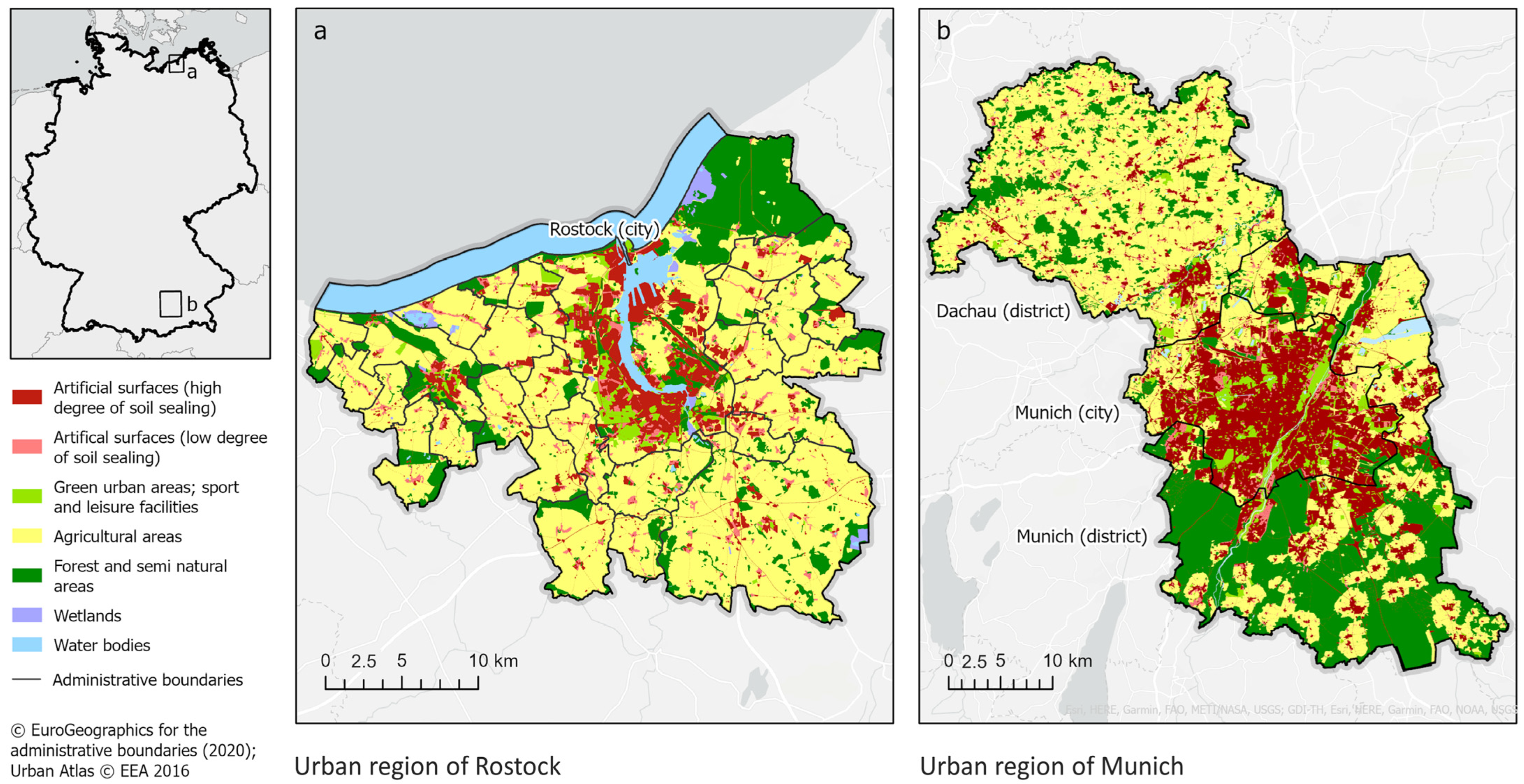
2.1. Study Areas

Selected ES of the two German urban regions of Rostock and Munich were mapped in this study. In both urban regions, dynamic urbanisation processes threaten the supply of multiple ES in periurban areas and increase the demand for ES in the urban areas. Figure 1 shows their location in Germany and the main LULC thematic classes of the freely available Urban Atlas data [44].
The urban region of Rostock is located in northeastern Germany in Mecklenburg–Western Pomerania. This study area encompasses 21 municipalities, including the city of Rostock. According to the European Nomenclature of Territorial Units for Statistics (NUTS), those municipalities correspond to Local Administrative Units (LAU) [45]. The study area covers approximately 670 km² and has a population of more than 270,000 inhabitants [46]. The dominant land-use type is agriculture (63%). The urban region of Rostock is an attractive place to live and work. Some smaller towns in its vicinity are experiencing strong population growth [47]. Owing to its location on the Baltic Sea coast, it is a popular destination for tourists and day visitors [48]. Another popular tourist attraction and important nature conservation area is Rostock Heath (a coastal forest and heathland region) east of Rostock.
The urban region of Munich is located in the southern Germany in Bavaria. The boundaries are delimited towards the regional NUTS3 level. This study area includes two districts, Dachau and Munich, and the city of Munich, which is the capital of Bavaria. This study area covers an area of approximately 1550 km² and has over 1.9 million inhabitants [46]. Agriculture (44%) is the dominant land-use type, followed by forest areas (27%). However, the city of Munich is primarily characterised by artificial surfaces and is densely built-up. Munich is an economically attractive location and one of the fastest-growing cities in Germany [47]. Despite being a densely built city, it has several parks, such as the English Garden along the River Isar, which are popular with the inhabitants and visitors. The district of Dachau extends from the northwestern suburbs of Munich. It is a hilly and agricultural-dominated countryside, with many villages and the city of Dachau. The urban sprawl extending from Munich is advancing into the district’s territory. The forest-dominated district of Munich is located to the east and south of the city. In the south is the highest elevation of the case-study area (approximately 700 m), announcing the Alpine foothills. The city’s growth is also strongly noticeable in this district, especially close to the city’s boundaries [49].
According to the Köppen–Geiger climate classification, both study areas are in climate class Cfa, which is characterised by a warm, temperate climate with humid periods, warm summers, and cold winters [50].

2.2. Selected Indicators

This study focused on five ES, which were selected based on their relevance for local stakeholders during workshops in the case-study regions [23]: (1) food (from cultivated terrestrial plants), (2) raw materials (from cultivated terrestrial plants), (3) pollination, (4) local climate regulation, and (5) coastal protection (see Table 1).

2.3. Definitions of ES Supply and Demand

We followed the understanding of ES supply and demand from the comprehensive MAES glossary [1]. Here, ES supply is defined as “the provision of a service by a particular ecosystem, irrespective of its actual use” [1]. ES demand can be described as “the need for specific ecosystem services by society, particular stakeholder groups, or individuals. It depends on factors such as culturally dependent desires and needs, availability of alternatives, or means to fulfil these needs. It also covers preferences for specific attributes of ecosystem services and relates to risk awareness” [1].

2.4. Methods

We selected ES mapping approaches following Martínez-Harms and Balvanera (2012) [52], Grêt-Regamey et al. (2015) [24], and the MAES Methods Explorer [53]. We chose (1) the expert-based ES matrix approach, (2) simple GIS mapping with proxy indicators and data, and (3) InVEST models as an example of more complex assessments. The results from simple GIS mapping and InVEST models were classified into the six 0–5 classes to face comparison with the expert estimates from the expert-based ES matrix approach. The classification was done manually and followed the recommendations by Burkhard et al. (2017) [27] and Schumacher et al. (2021) [30] (see Supplementary Materials S1).
If possible, we assessed and mapped ES supply and demand for all selected ES. We used ArcGIS Pro 2.9 for data preparation, mapping, and analysis. Table 2 shows an overview of the methods and indicators used. The following subsection briefly describes the methods used. More detailed descriptions of the data, indicators, methods, and InVEST models used are provided in Supplementary Materials S1.

2.4.1. Method 1: Expert-Based ES Matrix Approach

The experts’ estimates for ES supply and demand were collected with an empty matrix during topical workshops in Rostock and Munich [22,23], which followed the methodology for the ES matrix approach based on expert knowledge [54]. The matrix was structured as follows: The columns described selected ES, and the rows the thematic LULC classes of Urban Atlas (see Supplementary Materials S1). Local stakeholders were invited to estimate ES supply and demand using the scale 0–5 (from no relevant ES supply/demand to very high). Additionally, the participants were asked to score their confidence in their knowledge of each ES and LULC class using the scale 0–5 (very uncertain—very certain) [55]. Following Campagne et al. (2017) [55], we analysed the estimates using simple descriptive statistics and weighted the mean values with confidence scores. After that, a joint discussion among workshop participants took place. During these guided discussions, we took notes, clustered main arguments, and used them to interpret the results.

2.4.2. Method 2: Simple GIS Mapping

We used proxy indicators that relied only on a single data source: LULC, literature, or statistical data. Unfortunately, no suitable proxy data for assessing the ES supply for pollination or coastal protection could be found. The demand for coastal protection could be mapped with four different proxy indicators, representing the flood risk for the assets of human health, environment, infrastructure, and human economic activities [56].

2.4.3. Method 3: InVEST Models

For the selected ES, the following InVEST models are available:
  • Food (from cultivated terrestrial plants): Crop Production [57];
  • Pollination: Pollinator Abundance: Crop Pollination [57];
  • Locale climate regulation: Urban Cooling [58];
  • Coastal protection: Coastal Vulnerability [59].
However, owing to data availability reasons, we could only test the InVEST models Pollinator Abundance: Crop Pollination and Urban Cooling in more detail. More detailed descriptions of the InVEST models used are provided in Supplementary Materials S1. For mapping ES supply of and demand for raw materials, there are no InVEST models yet available [40].

2.4.4. Map Comparisons

The spatial differences between expert estimates and ES values from simple GIS mapping and InVEST models were detected through map comparisons. We compared the maps by calculating a similarity index for each ES. First, we normalised the expert estimates to a scale between 0 and 1 and converted each map into a raster (cell size: 10 ha). The calculation of the similarity index followed three steps [60]:
s(mapa, mapb) = mapa − mapb
where s represents the similarity values of mapa and mapb [60]. The absolute difference (s2) between mapa and mapb was calculated using:
s2(mapa, mapb) = con(s(mapa, mapb) < 0, s(mapa, mapb)* −1, s(mapa, mapb))
The absolute difference values were switched to similarity values using:
Similarity index = 1 − s2(mapa, mapb)

3. Results

Several challenges were encountered with all tested methods in both urban regions during the mapping processes. This resulted in different mapping outcomes of varying quality depending on the ES and the method used (see Table 3). The following subsections describe the results in more detail.

3.1. Method 1: Expert-Based ES Matrix Approach
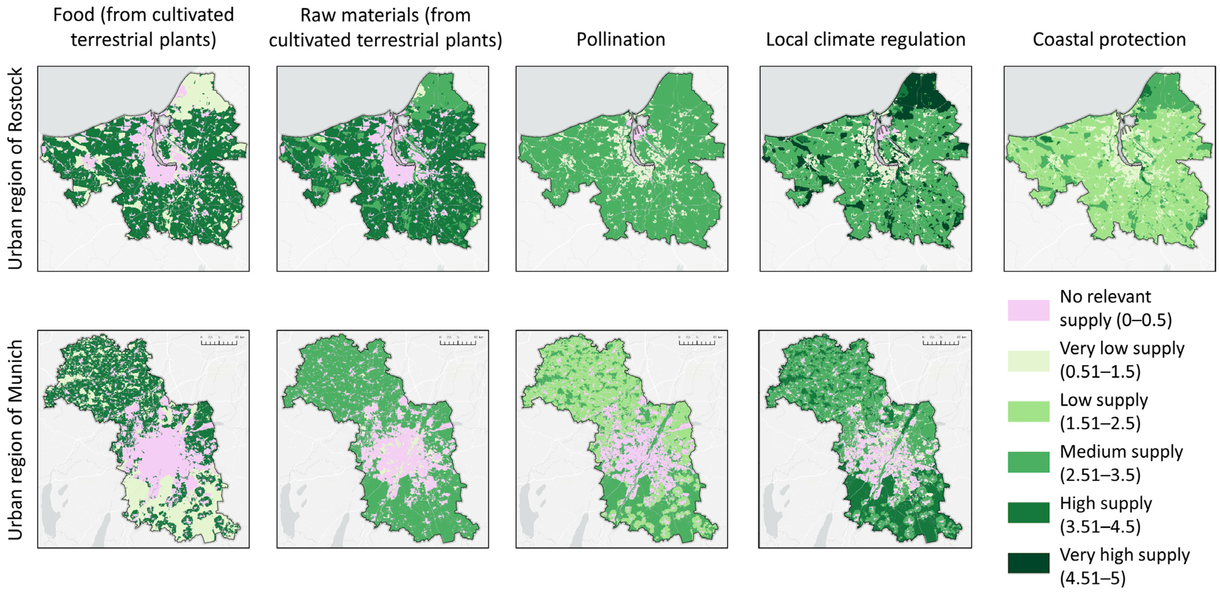
3.1.1. ES Supply

Fifteen local stakeholders had filled in the ES supply matrix for the urban region of Rostock, and twelve local stakeholders for the urban region of Munich (Supplementary Materials S2). The experts’ estimates showed to be similar for the selected provisioning ES. They differed for some LULC types, such as open vegetation areas. Estimates for regulating and maintenance services tended to be less consistent for some LULC types (e.g., flood protection in urban green areas). Participants representing the urban region of Rostock gave divergent estimations for the ES flood and coastal protection, which may indicate a comprehension issue for this ES.
Figure 2 shows the spatial pattern of ES supply. Overall, the maps show an urban–rural pattern, for example, low ES supply in built-up areas and high or very high in less anthropogenically altered areas such as forests or open vegetation areas. Furthermore, the results show that some ES, such as food, are strongly linked with specific LULC types.
Local stakeholders showed interest in the ES matrix approach and gave relevant feedback. For example, the participants suggested using more differentiated LULC data, especially in urban areas. Furthermore, they stated that estimations on a regional scale were difficult, as the urban regions contain rather heterogeneous landscapes. The participants from the urban region of Rostock requested the inclusion of coastal areas and the Baltic Sea and a more decisive distinction between coastal protection and flood protection.

3.1.2. ES Demand

The local stakeholders had difficulties comprehending the term ES demand and preferred not to fill in the blank matrix. As the ES demand matrices were missing, we could not generate maps indicating the spatial distribution of ES demand with this approach. Instead, joint discussions took place on ES demand. The workshop participants mentioned the following points during follow-up discussions as the biggest obstacles that made confident estimates via the expert-based ES matrix approach difficult:
  • For non-ES experts, the definition of ES demand was hard to understand.
  • The ES demand can be expressed by society, stakeholder groups, or individuals through wishes, values and norms, use or consumption patterns, or the need for risk reduction/prevention and increased security against natural hazards [15,56]. The stakeholders were divided on which perspective and types of demand should be considered.
  • Stakeholders found it challenging to estimate ES demand within the selected LULC, as they felt that demand originated from people and markets and not from the specific LULC types.
  • It was unclear how to estimate ES demand for provisioning ES, such as food, whose goods and products are transported and used worldwide. In this case, the stakeholders questioned whether a regional assessment of ES supply and demand would be helpful.
  • Stakeholders found it challenging to estimate the demand for regulating ES at a regional scale due to the more local scope of many ecosystem processes and functions that are underlying regulating ES.
  • The study regions were considered too large and too heterogeneous. The participants from the urban region of Munich especially emphasised this point.

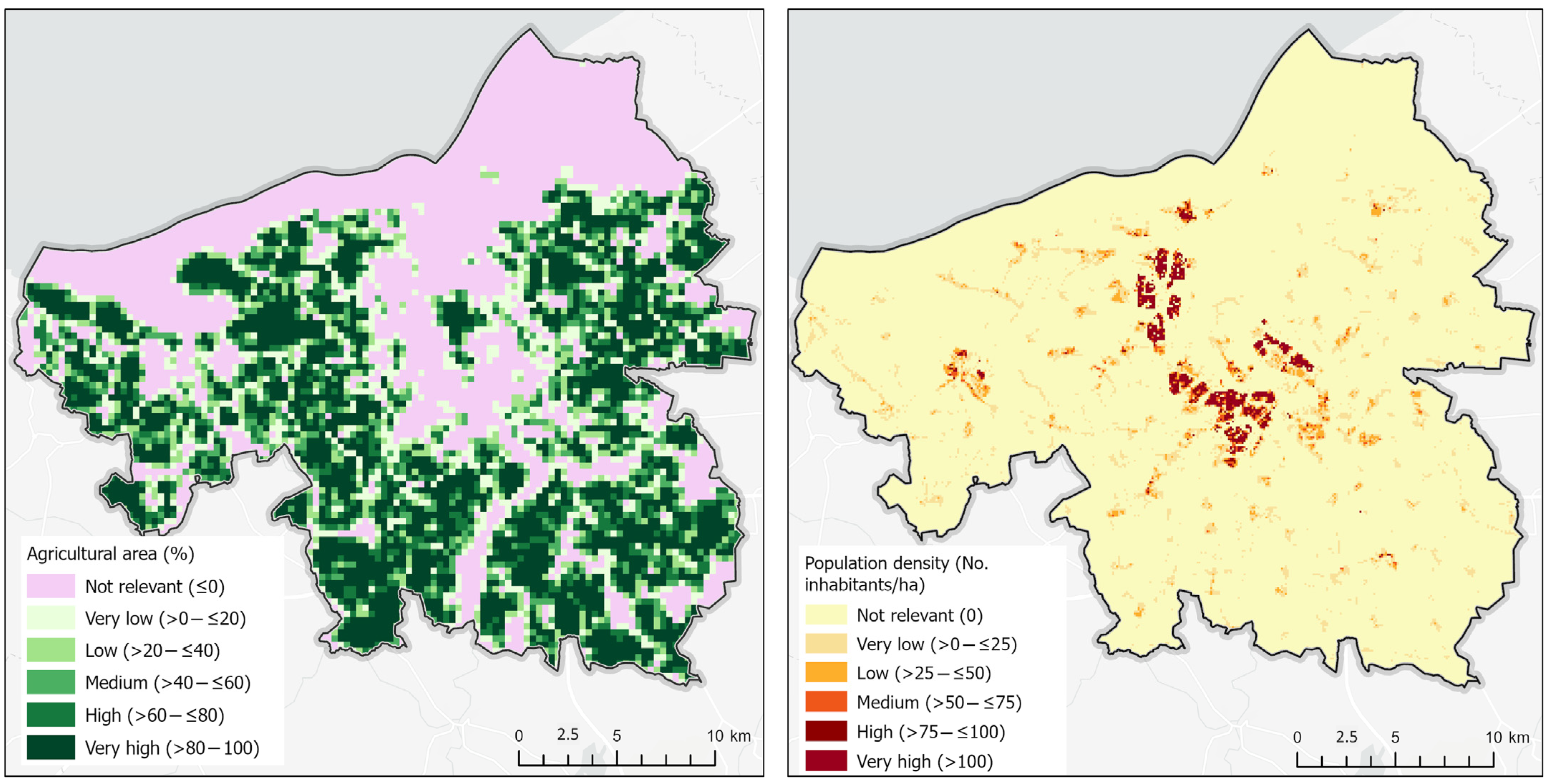
3.2. Method 2: Simple GIS Mapping

ES supply and demand were mapped with proxy indicators and data. The maps visualise distinctive spatial patterns and can potentially reflect service-providing or service-demanding areas. Figure 3 shows exemplary the ES supply of and demand for food using the indicators agricultural areas (%) and population density (inhabitants ha−1), respectively.
Several proxy indicators for coastal protection were used (see Figure 4). Those indicators express coastal flood risks for different protected assets (human health, infrastructure, environment, and human economic activities). In addition, the maps show detailed results of the assets at risk of coastal flooding at a local scale. The results highlight that ES demand can be located differently depending on the chosen indicator.

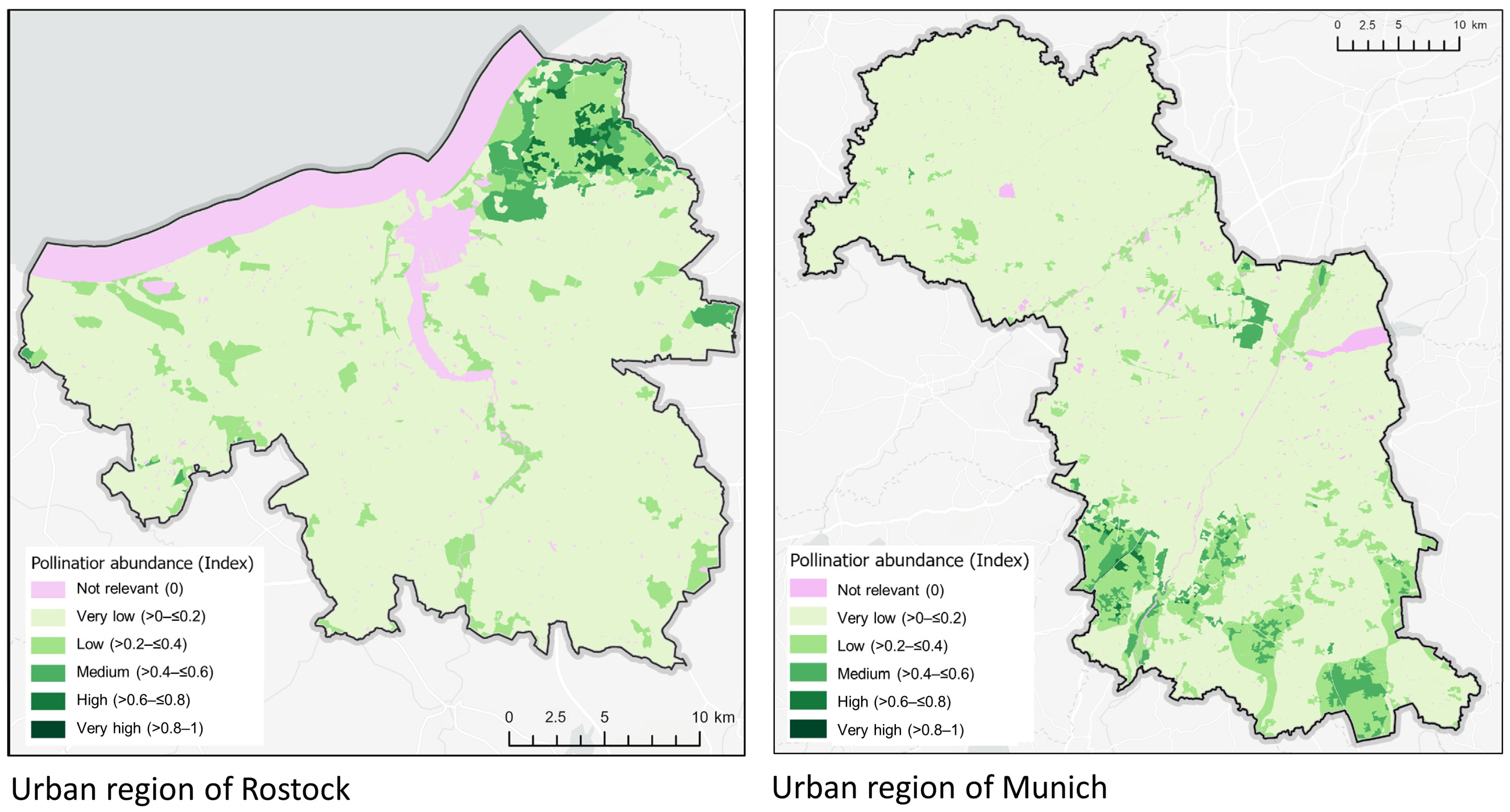
3.3. Method 3: InVEST

Only the InVEST models Pollinator Abundance: Crop Pollination and Urban Cooling could be run. Both models provided site-explicit results. Figure 5 shows exemplary the spatial patterns of potential ES supply for pollination, indicated with the indicator pollinator abundance (index). In both urban regions, only a few areas have medium to high ES supply. These areas are located in the most heterogeneous landscapes of urban regions. The models Crop Production [57] and Coastal Vulnerability [59] could have been suitable for mapping food and coastal protection, respectively. Furthermore, the model Pollinator Abundance: Crop Pollination provides an indicator for mapping ES demand. However, these models or indicators could not be calculated due to data availability reasons.

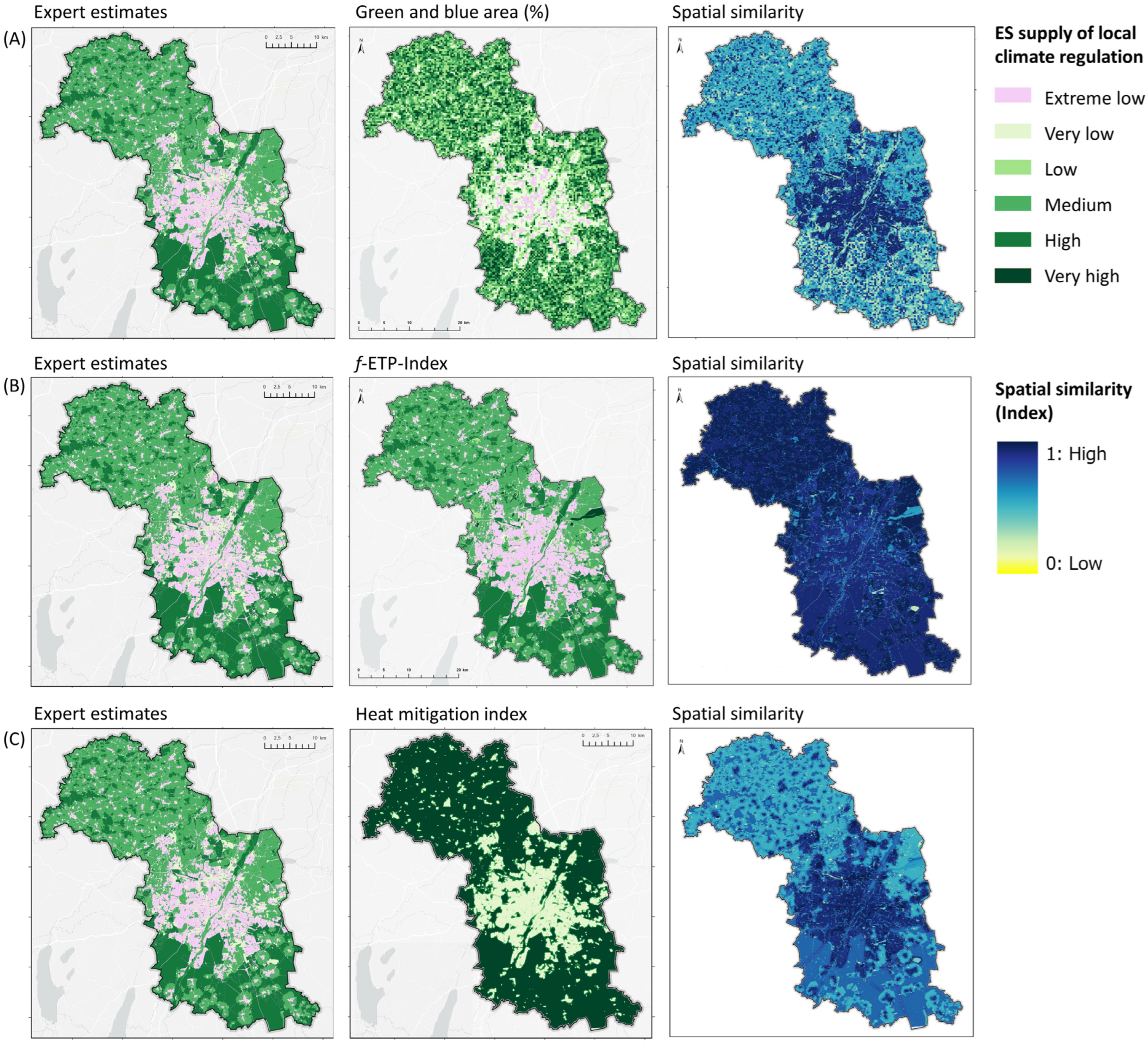
3.4. Map Comparison (Example: Local Climate Regulation)

We tested the spatial similarity between the expert estimates (results from the expert-based matrix approach), simple GIS mapping using proxy indicators and data, and InVEST models. In this section, we show exemplary results for local climate regulation in the urban region of Munich. Overall, the expert estimates differ to varying degrees from the other results (see Table 4 and Figure 6). The comparison between the expert estimates and the indicator green and blue area (%) (mean: 0.63), as well as between the expert estimates and InVEST results, expressed with the indicator heat mitigation index (mean: 0.69), show low spatial similarities. However, in both map comparisons, the spatial dissimilarities are distributed differently: The major dissimilarities are located in the case-study regions’ rural areas, whereas anthropogenically influenced areas show higher spatial similarity (see also Supplementary Materials S2).
High spatial similarity can be identified between expert estimates and indicator f-ETP (mean: 0.91). Both the expert estimates and the values of the indicator f-ETP were provided for each LULC type. The same data basis can explain the high degree of spatial similarity. However, the result also shows differences, especially in the LULC types water bodies and urban green spaces (see also Supplementary Materials S2).

4. Discussion

We aimed to map ES supply and demand with different ES relevant to the urban regions of Rostock and Munich. The information was needed for communicating and awareness-raising of the ES concept with local stakeholders during workshops and online meetings. We chose several easy-to-apply methods and tested their applicability in two case-study areas. During the ES mapping exercises, we dealt with challenges such as barriers related to understanding problems of the ES concept itself and the impact of data availability on selecting indicators and methods. These challenges, also known as “bottlenecks” [61], are well-known obstacles in ES mapping and have affected the mapping results to varying degrees.

4.1. How Useful Are Commonly Used ES Mapping Approaches in Regional Urban Contexts and What Major Obstacles to Their Application Did We Encounter?

4.1.1. Method 1: Expert-Based ES Matrix Approach

In the last 10–15 years, the ES matrix approach has been tested and updated in many applications [28]. Overall, the expert-based ES matrix approach has been appreciated for its comparably simple and fast technique that provides spatially explicit results on ES supply and demand [27,28,35]. We can only partially agree with this statement, as we could only record expert estimates for ES supply. ES demand can be expressed through different perspectives and demand types [62,63]. Consequently, there are broad possibilities for understanding ES demand [64]. This complexity hindered the local stakeholders’ making confident and comparable estimates [22].
Other uncertainties and limitations of the expert-based ES matrix approach are well documented, addressing, alongside other factors, the simplicity of application, experts and panel composition, statistical analyses, geodata used, and size of the case-study area [28,30,65,66]. The latter point was mentioned as a concern in both urban regions, as it reduced the confidence of local stakeholders. Furthermore, Campagne et al. (2017) elaborated that an expert panel size of at least 15 expert estimates is needed to provide reliable expert estimates [55]. Looking at the expert estimates for ES supply, the small number of local stakeholders who participated in Munich (n = 12) and Rostock (n = 15) can be a factor of uncertainty [66,67].

4.1.2. Method 2: Simple GIS Mapping

The simple GIS mapping with proxy indicators and data provided quick results, which show important spatial landscape information of ES supply and demand in the case-study areas. However, we faced obstacles in finding simple, suitable and recommended proxy indicators, and ES-related data for the regional scale.
Several indicators and data sets were of interest in the indicator selection process but could not be used since the needed data were unavailable/inaccessible or unsuitable for regional mapping. For example, the EU-wide working group Mapping and Assessment of Ecosystem and their Services (MAES) recommend well-tested indicators such as crop yield production, wood increment, or timber harvest [20,68], which are also integrated into the SEEA-EA framework [17]. For those indicators, national statistical data are freely available. This data are, however, too coarse to show the spatial patterns of ES supply or demand in the two urban regions [68,69]. Alternatively, we could have used the underlying high-resolution data from the local authorities. These data are, however, expensive or not easily accessible due to data protection reasons [63,70,71]. We could also map the MAES-recommended indicator dependence of crops on pollination by insects [20]. However, the corresponding literature data [72] can only be linked to cultivated crops on agricultural land. Hence, gapless mapping on the urban regional scale was not possible with this indicator.
Since we could not rely on the well-tested and recommended indicators for our selected ES, we used other alternative indicators and data. One of the simplest ways to map ES supply and demand is by using LULC types [36], despite its limited information content [66]. For example, the proportion of agricultural areas (%) can be linked to food supply (see Figure 3). This indicator cannot, however, communicate whether the areas are actually used for food cultivation, nor can the results show whether the land is being used sustainably [73]. Furthermore, using only certain LULC types as predictor variables neglects the capacity of other LULC types to provide ES [29]. Using highly generalised LULC types may not be appropriate for other ES, such as pollination or coastal protection. In these examples, more specific data on habitats, biotopes, or coastal ecosystems would be beneficial for informative ES mapping [30,74].
A transfer of ES values from literature data provides the opportunity to quickly generate cost-effective maps without using complex models. For this option, however, literature data need to be available for the respective ES in the first place. Suitable literature data were—to our knowledge—only available for the proxy indicators f-ETP and surface emissivity. The values originate from a study in Leipzig, Germany [75], and have been used in several urban case-study areas in Europe [76]. These two indicators also have the advantage of being available for the same datasets, similar spatial scales, and comparable units. This allows further ES mismatch analyses, which could indicate unsustainable use or inequitable distribution of ES [64,77]. However, for value transfer, the initial detailed modelling results were strongly generalised, which reduces the information content [75]. Furthermore, literature data only assumes that the ES values can be applied to case-study areas, even if the study purposes, temporal or spatial scales, data sources, or context-specific conditions differ [66].
Population density is an often used proxy indicator for visualising potential source–sink patterns [33,62]. We used this indicator for mapping demand for several ES, e.g., food or raw materials. However, ES demand is multifaceted and can cover desires/needs for specific attributes of ES or relates to risk awareness [1,64]. Using the same indicator for assessing and mapping the demand for several ES strongly reduces its inherent complexity. In comparison, the manifold patterns of ES demand for coastal protection had been mapped by considering the specific flood risks for protected assets (see Figure 4). The indicators (see Table 2) have the additional advantage that they are directly linked to the EU Floods Directive (Directive 2007/60/EC) [56,78].

4.1.3. Method 3: InVEST Models

The two tested InVEST models performed well in detecting spatial patterns of the individual ES and provided results with higher spatial resolution. The models can analyse how various parameters influence the supply of the respective ES [65]. For example, the model Pollinator Abundance: Crop Pollination calculates potential habitats and distribution of pollinating insects in a landscape [79]. Our results show that pollinator abundance is high in heterogeneous landscapes and low in homogenous agricultural areas. The results are, therefore, suitable to explain that ES supply can be increased by diversifying landscapes with insect-friendly structural elements.
The InVEST model Urban Cooling includes, in addition to LULC types, climate conditions and the distance to and size of urban green areas, and considers the possible spatial patterns of urban heat islands [58]. The modelled heat mitigation index can inform local stakeholders about the increased cooling capacity of larger urban parks and connected green infrastructure [12]. However, this model does not, for example, integrate the amount and/or the structure of green area quantifiably. Therefore, the results show no heat mitigation differences for forests or agricultural areas in the surroundings of the case-study area and might not be suitable for estimating the supply of local climate regulation on a regional scale.
Both tested models have several methodological uncertainties and limitations, which address the rule-based methodological design and the limited capability for calibration and validation [12,43,79]. As for all model computations, the input data resolution and quality affect the results strongly [65]. As mentioned in the results, we could not run the models Coastal Vulnerability, Crop Production, and the demand component of Pollinator Abundance: Crop Pollination due to data availability reasons.

4.1.4. Map Comparisons

Model results are often interpreted as “more correct” than the results of proxies or expert estimates, even if the accuracy, input data, or reliability of the models used are questionable [80]. However, the map comparisons show that the expert-based ES matrix approach can detect similar spatial patterns of ES supply on the regional scale. Dissimilarities can be explained by the proxy indicator chosen and its informational content, different spatial resolutions of the data sources, and the calculations within the InVEST model Urban Cooling [58]. The model results show no heat mitigation differences on nonurban LULC types, which can explain the greater spatial dissimilarities on those areas.

4.2. How Can Our Experiences Help Inform Future Research and Related Application Perspectives in ES Mapping?

Overall, mapping ES supply and demand at the spatial scale and resolution of urban and periurban areas was challenging for all methodological approaches. We could only map ES supply and demand for some selected ES with simple GIS mapping using proxy indicators and data, or with InVEST model outcomes. Recommended and tested indicators and accessible data were, unfortunately, still missing [64]. Comparably simple ES models such as InVEST provide—if available for the selected ES and spatial scale—more site-specific results. The results show more deeply the interactions between the ES components and/or socioecological processes in the chosen case-study areas. However, running the models demands time and is data intensive, and already requires an in-depth understanding of the respective ES.
The most decisive advantage of the expert-based ES matrix approach is that this approach provides opportunities for communication and discussions with local stakeholders as early as during the collection of the expert estimates. Dialogue between science and policy are important to capture local stakeholders’ and decision-makers’ interests and needs [9,61,67]. For instance, the local stakeholders questioned the point of mapping ES demand for provisioning ES (such as food), as the demand cannot be reduced easily through, for example, urban or regional planning instruments. Overall, the multifaceted nature of ES demand proved to be a hurdle in participatory ES mapping approaches. For future expert-based ES matrix applications, we recommend alternative methodological designs that use questionnaires and joint discussions instead of a blank matrix. Overall, the discussions on ES demand revealed that this component needs a clarified understanding and further research. Despite the drawbacks on the subject of ES demand, the workshops and discussions were of high relevance (and perhaps equally important than the final maps [67]), as they helped to promote a better understanding of the ES concept amongst the local stakeholders [28,41,81].
It would be advantageous to utilise better the connections to existing legislations or consolidated approaches within the ES concept. Using ES indicators and data [78,82], which are also applied in policies such as the EU Floods Directive (Directive 2007/60/EC), can increase the impact of the ES concept together with the understanding and acceptance of the results amongst local stakeholders [56]. Furthermore, other approaches, such as lifecycle assessments [83,84,85], ecological footprints [86,87], or the emergy evaluation methodology [88,89], have been developed and broadly applied to highlight the contribution of nature and the origin of the natural resources used or the impacts of human activities on natural resources. In particular, lifecycle assessments and ecological footprints are excellent communication and awareness-raising tools [89]. The methodologies could be used as alternative approaches for assessing the teleconnections between urban and periurban areas [90], ES flows [91,92], and ES demand for provisioning ES and selected regulating and cultural ES [84]. Initial ideas for an integration of the lifecycle assessment or ecological footprints into the ES cascade framework exist, but still need to be developed further [85,93]. For greater impact in spatial planning and governance processes, site-specific results at different spatial scales and the integration of further ES are needed [89,93].

5. Conclusions

This study summarised conceptual and methodological challenges that entailed applying different ES supply and demand mapping approaches during a research project in Germany. The expert-based ES matrix approach provided results on ES supply and detected comparable distinctive spatial ES supply patterns. However, the conceptual complexity of ES demand hampered the participants in making confident estimates on the subject of ES demand. Nevertheless, dialogues with practitioners and local stakeholders were important to capture interests and needs as well as existing barriers that impact the use of the ES concept in real-world decisions.
Simple GIS mapping with proxy indicator and data and the use of InVEST models were accompanied by barriers related to indicator selection, method, and data unavailability/inaccessibility. Recommended and well-tested indicators, which can be applied relatively quickly with simple mapping approaches, are still missing for many ES. These approaches are needed when overviews about ES-related topics are requested for communication and awareness-raising, and when time and/or financial constraints prevent a more in-depth analysis. Future research needs to provide more agreed indicators together with standardised quantification methods to enable both ES supply and demand assessments on comparable spatial scales. With this study and by sharing our experience in mapping selected ES with commonly applied methods, we hope to contribute to fill the gap between scientific state-of-the-art contributions and actual user needs.

Supplementary Materials

The following supporting information can be downloaded at: https://www.mdpi.com/article/10.3390/land12010052/s1, S1: Table S1. Data used for the ES supply/demand mapping and assessments. Table S2. Overview of the indicators, methods, and categorisation used. If possible, indicators were mapped at a regional scale. Table S3. Overview of the indicators used in the ES modelling. If possible, indicators were mapped at a regional scale. Table S4. Selected LULC classes from CORINE Land Cover (CLC) and Urban Atlas. Table S5. Biophysical table, adapted from Zulian et al. (2013). Marked LULC (*) shows adjusted values for the Urban Atlas dataset. Table S6. Guide table for the InVEST model Pollinator Abundance: Crop Pollination. Table S7. Pollination dependencies (%) of crops that could grow on selected LULC (adapted from Zulian et al. (2013)). Table S8. Biophysical table for the InVEST model Urban Cooling, urban region of Munich. Table S9. Biophysical table for the InVEST model Urban Cooling, urban region of Rostock. Table S10. Classification of flood hazard. Tables S11–S14. Classification of the potential damage for the asset human health, environment, infrastructure, and economic activities. Table S15. Classification of the coastal flood risks into six ES classes. Figure S1. Standardised Kc values for CORINE Land Cover and Urban Atlas, adapted from Nistor (2018 and 2016). S2: Table S16. Expert-based ES matrix approach, ES supply, urban region of Rostock, n = 15. Weighted mean values. Table S17. Expert-based ES matrix approach, ES supply, urban region of Munich, n = 12. Weighted mean values. Tables S18–S20. Similarity values of the map comparison between the maps from expert estimates (expert-based ES matrix approach) and the indicator (A) green and blue area (%) (LULC data), (B) f-ETP-Index (literature data), (C) heat mitigation index (InVEST model Urban Cooling) in the urban region of Munich. The value 0 indicates no similarity, and 1 very high similarity between the compared maps. Figures S2–S6. Expert estimates of ES food (from cultivated terrestrial plants), raw materials (from cultivated terrestrial plants), pollination, local climate regulation, and, flood and coastal protection. Urban region of Rostock. Figures S7–S10. Expert estimates of ES food (from cultivated terrestrial plants), raw materials (from cultivated terrestrial plants), pollination, and, local climate regulation. Urban region of Munich. Figure S11. Food (from cultivated terrestrial plants). Indicator: Agricultural area (%). Urban region of Rostock. Figure S12. Food (from cultivated terrestrial plants). Indicator: Population density (Inhabitants ha−1). Urban region of Rostock. Figure S13. Pollination. Indicator: Pollinator Abundance (Index 0 to 1). Urban region of Rostock. Figure S14. Pollination. Indicator: Pollinator Abundance (Index 0 to 1). Urban region of Munich. Figures S15–S18. Coastal protection, mapped with the indicators: Human health at risk of coastal flooding; Infrastructure at risk of coastal flooding; Environment (biotopes) at risk of coastal flooding; Human economic activities at risk of coastal flooding. Urban region of Rostock. Figure S19. Local climate regulation. Indicator: Green and blue area (%). Urban region of Munich. Figure S20. Local climate regulation. Indicator: f-evapotranspiration (f-ETP) (Index 0 to 1). Urban region of Munich. Figure S21. Local climate regulation. Indicator: Heat mitigation (Index 0 to 1). Urban region of Munich. References [94,95,96,97,98,99,100,101,102,103,104,105,106,107,108,109,110,111] are cited in the supplementary materials.

Author Contributions

Conceptualization, C.D. and B.B.; methodology, C.D.; software, C.D.; formal analysis, C.D.; investigation, C.D.; resources, C.D.; data curation, C.D.; writing—original draft preparation, C.D.; writing—review and editing, C.D. and B.B.; visualization, C.D.; supervision, C.D.; project administration, C.D. and B.B.; funding acquisition, B.B. All authors have read and agreed to the published version of the manuscript.

Funding

The Federal German Ministry of Education and Research (BMBF) funded the OESKKIP research project within the framework of the strategy ‘Research for Sustainability’ (FONA—Forschung für Nachhaltige Entwicklung) (FKZ 16LC1604B).

Data Availability Statement

Publicly available datasets were analysed in this study. These data can be found here: Eurostat. 2022. Countries. Available online: https://ec.europa.eu/eurostat/web/gisco/geodata/reference-data/administrative-units-statistical-units/countries#countries20 (accessed on 2 April 2022). European Environment Agency. 2016. Urban Atlas 2012. Available online: https://land.copernicus.eu/local/urban-atlas/urban-atlas-2012?tab=metadata (accessed on 2 April 2022). European Environment Agency. 2019. Corine Land Cover (CLC) 2012. Available online: https://land.copernicus.eu/pan-european/corine-land-cover/clc-2012?tab=metadata (accessed on 2 April 2022). Statistisches Bundesamt. 2015. Ergebnisse des Zensus 2011 zum Download—erweitert. Available online: https://www.zensus2011.de/DE/Home/Aktuelles/DemografischeGrunddaten.html;jsessionid=6E45AA84910CD1717DDD8A2D100A5DE1.1_cid380?nn=3065474 (accessed on 2 April 2022). Bundesamt für Kartographie und Geodäsie. 2020. Geographische Gitter für Deutschland in Lambert-Projektion (GeoGitter Inspire). Available online: https://gdz.bkg.bund.de/index.php/default/digitale-geodaten.html (accessed on 2 April 2022). European Environment Agency. 2018. Tree Cover Density. Available online: https://land.copernicus.eu/pan-european/high-resolution-layers/forests/tree-cover-density (accessed on 2 April 2022). Climate Data Center. 2020. Datensatzbeschreibung. Monatliche Raster der potenziellen Evapotranspiration über Gras, Version 0.x. Available online: https://opendata.dwd.de/climate_environment/CDC/grids_germany/monthly/evapo_p/BESCHREIBUNG_gridsgermany_monthly_evapo_p_de.pdf (accessed on 2 April 2022). Climate Data Center. 2019. Berechnete monatliche Werte von charakteristischen Elementen aus dem Boden und dem Pflanzenbestand., Version v19.3. Available online: https://opendata.dwd.de/climate_environment/CDC/derived_germany/soil/monthly/historical/BESCHREIBUNG_derivgermany_soil_monthly_historical_de.pdf (accessed on 2 April 2022). Climate Data Center. 2018. Historische tägliche Stationsbeobachtungen (Temperatur, Druck, Niederschlag, Sonnenscheindauer, etc.) für Deutschland. Available online: https://opendata.dwd.de/climate_environment/CDC/observations_germany/climate/daily/kl/historical/ (accessed on 2 April 2022). Yale University. 2019. Global Surface UHI Explorer. Available online: https://yceo.yale.edu/research/global-surface-uhi-explorer (accessed on 2 April 2022). Restrictions apply to the availability of some data. ATKIS and the digital elevation model were obtained from Landesamt für innere Verwaltung Mecklenburg–Vorpommern and are available at https://www.laiv-mv.de/Geoinformation/Geobasisdaten/ (accessed on 2 April 2022) with the permission of Landesamt für innere Verwaltung Mecklenburg-Vorpommern (2018). Coastal flood risk data were obtained from Landesamt für Umwelt, Naturschutz und Geologie M-V and are available at https://www.umweltkarten.mv-regierung.de/atlas/script/index.php (accessed on 2 April 2022) with the permission of Landesamt für Umwelt, Naturschutz und Geologie M-V. The expert estimates presented in this study are available in Supplementary Materials S1.

Acknowledgments

We would like to thank the whole OESKKIP project team and the participating stakeholders for their highly valuable contributions. Many thanks go to Thea Wübbelmann and Nadja Kabisch for helpful discussions and to Ann Cruickshank and Matthew Cruickshank for English proofreading.

Conflicts of Interest

The authors declare no conflict of interest. The funders had no role in the design of the study; in the collection, analyses, or interpretation of data; in the writing of the manuscript, or in the decision to publish the results.

References

  1. Potschin-Young, M.; Burkhard, B.; Czúcz, B.; Santos-Martín, F. Glossary of ecosystem services mapping and assessment terminology. One Ecosyst. 2018, 3, e27110. [Google Scholar] [CrossRef]
  2. The Economics of Ecosystems and Biodiversity. In The Economics of Ecosystems and Biodiversity: Mainstreaming the Economics of Nature: A Synthesis of the Approach, Conclusions and Recommendations of TEEB; UNEP: Geneva, Switzerland, 2010; ISBN 9783981341034.
  3. Millennium Ecosystem Assessment. In Ecosystems and Human Well-Being: Synthesis; Island Press: Washington DC, USA, 2005; ISBN 1597260398.
  4. IPBES. Summary for Policymakers of the Global Assessment Report on Biodiversity and Ecosystem Services of the Intergovernmental Science-Policy Platform on Biodiversity and Ecosystem Services; Díaz, S., Settele, J., Brondízio, E.S., Ngo, H.T., Guèze, M., Agard, J., Arneth, A., Balvanera, P., Brauman, K.A., Butchart, S.H.M., et al., Eds.; IPBES secretariat: Bonn, Germany, 2019; ISBN 978-3-947851-13-3. [Google Scholar]
  5. European Commission. An Advocacy Toolkit for Nature. Biodiversity Loss, Nature Protection, and the EU Strategy for Nature; European Commission: Brussels, Belgium, 2021. [Google Scholar]
  6. Bolound, P.; Hunhammar, S. Ecosystem services in urban areas. Ecol. Econ. 1999, 29, 293–301. [Google Scholar] [CrossRef]
  7. Sylla, M.; Hagemann, N.; Szewrański, S. Mapping trade-offs and synergies among peri-urban ecosystem services to address spatial policy. Environ. Sci. Policy 2020, 112, 79–90. [Google Scholar] [CrossRef]
  8. Sloggy, M.R.; Escobedo, F.J.; Sánchez, J.J. The Role of Spatial Information in Peri-Urban Ecosystem Service Valuation and Policy Investment Preferences. Land 2022, 11, 1267. [Google Scholar] [CrossRef]
  9. Grunewald, K.; Bastian, O.; Louda, J.; Arcidiacono, A.; Brzoska, P.; Bue, M.; Cetin, N.I.; Dworczyk, C.; Dubova, L.; Fitch, A.; et al. Lessons learned from implementing the ecosystem services concept in urban planning. Ecosyst. Serv. 2021, 49, 101273. [Google Scholar] [CrossRef]
  10. Olander, L.; Polasky, S.; Kagan, J.S.; Johnston, R.J.; Wainger, L.; Saah, D.; Maguire, L.; Boyd, J.; Yoskowitz, D. So you want your research to be relevant? Building the bridge between ecosystem services research and practice. Ecosyst. Serv. 2017, 26, 170–182. [Google Scholar] [CrossRef]
  11. Tezer, A.; Turkay, Z.; Uzun, O.; Terzi, F.; Koylu, P.; Karacor, E.; Okay, N.; Kaya, M. Ecosystem services-based multi-criteria assessment for ecologically sensitive watershed management. Environ. Dev. Sustain. 2020, 22, 2431–2450. [Google Scholar] [CrossRef]
  12. Ronchi, S.; Salata, S.; Arcidiacono, A. Which urban design parameters provide climate-proof cities? An application of the Urban Cooling InVEST Model in the city of Milan comparing historical planning morphologies. Sustain. Cities Soc. 2020, 63, 102459. [Google Scholar] [CrossRef]
  13. The Economics of Ecosystems and Biodiversity. In Guidance Manual for TEEB Country Studies. Version 1.0.; United Nations Environment Programme: Geneva, Switzerland, 2013.
  14. European Union. Natural Capital Accounting: Overview and Progress in the European Union; Publications Office of the European Union: Luxembourg, 2019; ISBN 978-92-79-89744-3. [Google Scholar]
  15. European Commission. The EU Biodiversity Strategy to 2020; Publications Office of the European Union: Luxembourg, 2011; ISBN 9789279207624. [Google Scholar]
  16. European Commission. EU Biodiversity Strategy for 2030. Bringing Nature Back into Our Lives: COM/2020/380 Final; European Commission: Brussels, Belgium, 2020. [Google Scholar]
  17. United Nations. System of Environmental Economic Accounting—Ecosystem Accounting: Final Draft; United Nations: Geneva, Switzerland, 2021. [Google Scholar]
  18. Deppisch, S.; Heitmann, A.; Savaşçı, G.; Lezuo, D. Ökosystemleistungen in Instrumenten der Stadt- und Regionalplanung. RuR 2021, 80, 58–79. [Google Scholar] [CrossRef]
  19. Geneletti, D.; Adem Esmail, B.; Cortinovis, C.; Arany, I.; Balzan, M.; van Beukering, P.; Bicking, S.; Borges, P.; Borisova, B.; Broekx, S.; et al. Ecosystem services mapping and assessment for policy- and decision-making: Lessons learned from a comparative analysis of European case studies. One Ecosyst. 2020, 5. [Google Scholar] [CrossRef]
  20. Maes, J.; Teller, A.; Erhard, M.; Condé, S.; Vallecillo, S.; Barredo, J.I.; Paracchini, M.L.; Abdul Malak, D.; Trombetti, M.; Vigiak, O.; et al. Mapping and Assessment of Ecosystems and Their Services: An EU Ecosystem Assessment; Publications Office of the European Union: Luxembourg, 2020. [Google Scholar]
  21. OESKKIP. Integration of Ecosystem Services in Urban and Regional Planning. Available online: https://www.öskkip.de/?lang=en (accessed on 2 April 2022).
  22. Barkmann, T.; Heitmann, A.; Wessels, A.; Dworczyk, C.; Matschiner, J.; Neumann, C.; Savaşçı, G.; Burkhard, B.; Deppisch, S. Ökosystemleistungen in den Stadtregionen: Angebot, Nachfrage und Planungsrelevanz—Bericht Über die Durchführung und Ergebnisse der zweiten Workshopreihe in den Pilot-Stadtregionen Rostock und München; landmetamorphosis: Hamburg, Germany, 2020; ISBN 978-3-947972-02-9. [Google Scholar]
  23. Barkmann, T.; Wessels, A.; Dworczyk, C.; Burkhard, B.; Deppisch, S.; Matschiner, J. Angebot und Bedeutung von Ökosystemleistungen in Stadtregionen; landmetamorphosis: Hamburg, Germany, 2019; ISBN 978-3-941722-96-5. [Google Scholar]
  24. Grêt-Regamey, A.; Weibel, B.; Kienast, F.; Rabe, S.-E.; Zulian, G. A tiered approach for mapping ecosystem services. Ecosyst. Serv. 2015, 13, 16–27. [Google Scholar] [CrossRef]
  25. Grêt-Regamey, A.; Weibel, B.; Rabe, S.E.; Burkhard, B. A tiered approach for ecosystem services mapping. In Mapping Ecosystem Services; Burkhard, B., Maes, J., Eds.; Pensoft Publishers: Sofia, Bulgaria, 2017; pp. 211–215. ISBN 9789546428295. [Google Scholar]
  26. Burkhard, B.; Kroll, F.; Müller, F.; Windhorst, W. Landscapes’ capacities to provide ecosystem services—A concept for land-cover based assessments. Landscape Online 2009, 15, 1–22. [Google Scholar] [CrossRef]
  27. Burkhard, B. Ecosystem services matrix. In Mapping Ecosystem Services; Burkhard, B., Maes, J., Eds.; Pensoft Publishers: Sofia, Bulgaria, 2017; pp. 225–230. ISBN 9789546428295. [Google Scholar]
  28. Campagne, C.S.; Roche, P.; Müller, F.; Burkhard, B. Ten years of ecosystem services matrix: Review of a (r)evolution. One Ecosyst. 2020, 5, e51103. [Google Scholar] [CrossRef]
  29. Czúcz, B.; Arany, I.; Potschin-Young, M.; Bereczki, K.; Kertész, M.; Kiss, M.; Aszalós, R.; Haines-Young, R. Where concepts meet the real world: A systematic review of ecosystem service indicators and their classification using CICES. Ecosyst. Serv. 2018, 29, 145–157. [Google Scholar] [CrossRef]
  30. Schumacher, J.; Lange, S.; Müller, F.; Schernewski, G. Assessment of Ecosystem Services across the Land–Sea Interface in Baltic Case Studies. Appl. Sci. 2021, 11, 11799. [Google Scholar] [CrossRef]
  31. Burkhard, B.; Kandziora, M.; Hou, Y.; Müller, F. Ecosystem service potentials, flows and demands-concepts for spatial localisation, indication and quantification. Landscape Online 2014, 34, 1–32. [Google Scholar] [CrossRef]
  32. Goldenberg, R.; Kalantari, Z.; Cvetkovic, V.; Mörtberg, U.; Deal, B.; Destouni, G. Distinction, quantification and mapping of potential and realized supply-demand of flow-dependent ecosystem services. Sci. Total Environ. 2017, 593–594, 599–609. [Google Scholar] [CrossRef]
  33. Burkhard, B.; Kroll, F.; Nedkov, S.; Müller, F. Mapping ecosystem service supply, demand and budgets. Ecol. Indic. 2012, 21, 17–29. [Google Scholar] [CrossRef]
  34. Jacobs, S.; Burkhard, B.; van Daele, T.; Staes, J.; Schneiders, A. ‘The Matrix Reloaded’: A review of expert knowledge use for mapping ecosystem services. Ecol. Model. 2015, 295, 21–30. [Google Scholar] [CrossRef]
  35. Harrison, P.A.; Dunford, R.; Barton, D.N.; Kelemen, E.; Martín-López, B.; Norton, L.; Termansen, M.; Saarikoski, H.; Hendriks, K.; Gómez-Baggethun, E.; et al. Selecting methods for ecosystem service assessment: A decision tree approach. Ecosyst. Serv. 2017, 29, 481–498. [Google Scholar] [CrossRef]
  36. Burkhard, B.; Maes, J. (Eds.) Mapping Ecosystem Services; Pensoft Publishers: Sofia, Bulgaria, 2017; ISBN 9789546428295. [Google Scholar]
  37. Jacobs, S.; Verheyden, W.; Dendoncker, N. Why to map? In Mapping Ecosystem Services; Burkhard, B., Maes, J., Eds.; Pensoft Publishers: Sofia, Bulgaria, 2017; pp. 171–175. ISBN 9789546428295. [Google Scholar]
  38. Roche, P.K.; Campagne, C.S. Are expert-based ecosystem services scores related to biophysical quantitative estimates? Ecol. Indic. 2019, 106, 105421. [Google Scholar] [CrossRef]
  39. Maes, J.; Fabrega, N.; Zulian, G.; Barbosa, A.; Vizcaino, P.; Ivits, E.; Polce, C.; Vandecasteele, I.; Rivero, I.M.; Guerra, C.; et al. Mapping and Assessment of Ecosystems and Their Services: Trends in Ecosystems and Ecosystem Services in the European Union between 2000 and 2010; Publications Office: Luxembourg, 2015; ISBN 9279462067. [Google Scholar]
  40. The Natural Capital Project. InVEST. Available online: https://naturalcapitalproject.stanford.edu/software/invest (accessed on 24 February 2021).
  41. Van Oudenhoven, A.P.; Schröter, M.; Drakou, E.G.; Geijzendorffer, I.R.; Jacobs, S.; van Bodegom, P.M.; Chazee, L.; Czúcz, B.; Grunewald, K.; Lillebø, A.I.; et al. Key criteria for developing ecosystem service indicators to inform decision making. Ecol. Indic. 2018, 95, 417–426. [Google Scholar] [CrossRef]
  42. Ma, L.; Bicking, S.; Müller, F. Mapping and comparing ecosystem service indicators of global climate regulation in Schleswig-Holstein, Northern Germany. Sci. Total Environ. 2019, 648, 1582–1597. [Google Scholar] [CrossRef] [PubMed]
  43. Decsi, B.; Ács, T.; Jolánkai, Z.; Kardos, M.K.; Koncsos, L.; Vári, Á.; Kozma, Z. From simple to complex—Comparing four modelling tools for quantifying hydrologic ecosystem services. Ecol. Indic. 2022, 141, 109143. [Google Scholar] [CrossRef]
  44. European Environment Agency. Urban Atlas 2012. Available online: https://land.copernicus.eu/local/urban-atlas/urban-atlas-2012?tab=metadata (accessed on 22 March 2022).
  45. Maes, J.; Zulian, G.; Thijssen, M.; Castell, C.; Baró, F.; Ferreira, A.M.; Melo, J.; Garrett, C.P.; David, N.; Alzetta, C.; et al. Mapping and Assessment of Ecosystems and Their Services: Urban Ecosystems; 4th Report; Office for Official Publications of the European Communities: Luxembourg, 2016. [Google Scholar]
  46. Statistisches Bundesamt. Daten aus dem Gemeindeverzeichnis. Gemeinden mit 5000 und mehr Einwohnern nach Fläche, Bevölkerung und Bevölkerungsdichte. Available online: https://www.destatis.de (accessed on 15 February 2022).
  47. Bundesinstitut für Bau-, Stadt-, und Raumforschung. Wachsen und Schrumpfen von Städten und Gemeinden im Zeitintervall 2013–2018 im Bundesweiten Vergleich. Available online: https://www.bbsr.bund.de/BBSR/DE/startseite/topmeldungen/2020-wachsend-schrumpfend.html (accessed on 15 February 2022).
  48. Statista. Städte-Ranking Nach den Meisten Gästeübernachtungen je Einwohner in Deutschland im Jahr 2015. Available online: https://de.statista.com/statistik/daten/studie/538604/umfrage/meiste-gaesteuebernachtungen-je-einwohner-in-deutschland/ (accessed on 9 June 2022).
  49. Bayerisches Landesamt für Umwelt. Naturräumliche Gliederung Bayerns. Available online: https://www.lfu.bayern.de/natur/naturraeume/index.htm (accessed on 15 April 2021).
  50. Kottek, M.; Grieser, J.; Beck, C.; Rudolf, B.; Rubel, F. World Map of the Köppen-Geiger climate classification updated. metz 2006, 15, 259–263. [Google Scholar] [CrossRef]
  51. Haines-Young, R.; Potschin, M.B. Common International Classification of Ecosystem Services (CICES) V5.1 and Guidance on the Application of the Revised Structure. Available online: www.cices.eu (accessed on 15 October 2022).
  52. Martínez-Harms, M.J.; Balvanera, P. Methods for mapping ecosystem service supply: A review. Int. J. Biodivers. Sci. Ecosyst. Serv. Manag. 2012, 8, 17–25. [Google Scholar] [CrossRef]
  53. ESMERALDA. Welcome to the MAES Methods Explorer. Available online: http://database.esmeralda-project.eu/home (accessed on 17 April 2022).
  54. Campagne, C.S.; Roche, P. May the matrix be with you!: Guidelines for the application of expert-based matrix approach for ecosystem services assessment and mapping. One Ecosyst. 2018, 3, e24134. [Google Scholar] [CrossRef]
  55. Campagne, C.S.; Roche, P.; Gosselin, F.; Tschanz, L.; Tatoni, T. Expert-based ecosystem services capacity matrices: Dealing with scoring variability. Ecol. Indic. 2017, 79, 63–72. [Google Scholar] [CrossRef] [Green Version]
  56. INTEK. Integriertes Entwässerungskonzept (INTEK). Fachkonzept zur Anpassung der Entwässerungssysteme an die Urbanisierung und den Klimawandel. Phase 3: Einzugsgebietsbezogene Analysen der Hochwasserrisiken. Biota: Bützow, Germany. 2014. Available online: https://rathaus.rostock.de/media/rostock_01.a.4984.de/datei/Endbericht_INTEK_Phase3%20Risiko.pdf (accessed on 15 October 2022).
  57. NatCap. Crop Production. Available online: https://invest-userguide.readthedocs.io/en/latest/crop_production.html (accessed on 15 July 2022).
  58. The Natural Capital Project. Urban Cooling Model. Available online: http://releases.naturalcapitalproject.org/invest-userguide/latest/urban_cooling_model.html (accessed on 2 July 2020).
  59. The Natural Capital Project. Coastal Vulnerability Model. Available online: https://storage.googleapis.com/releases.naturalcapitalproject.org/invest-userguide/latest/coastal_vulnerability.html (accessed on 4 May 2021).
  60. Hagen-Zanker, A.; Engelen, G.; Hurkens, J.; Vanhout, R.; Uljee, I. Map Comparison Kit 3: User Manual. Environ. Model. Softw. 2006, 21, 346–358. [Google Scholar]
  61. Palomo, I.; Willemen, L.; Drakou, E.; Burkhard, B.; Crossman, N.; Bellamy, C.; Burkhard, K.; Campagne, C.S.; Dangol, A.; Franke, J.; et al. Practical solutions for bottlenecks in ecosystem services mapping. One Ecosyst. 2018, 3, e20713. [Google Scholar] [CrossRef] [Green Version]
  62. Wolff, S.; Schulp, C.; Verburg, P.H. Mapping ecosystem services demand: A review of current research and future perspectives. Ecol. Indic. 2015, 55, 159–171. [Google Scholar] [CrossRef]
  63. Wolff, S.; Schulp, C.; Kastner, T.; Verburg, P.H. Quantifying Spatial Variation in Ecosystem Services Demand: A Global Mapping Approach. Ecol. Econ. 2017, 136, 14–29. [Google Scholar] [CrossRef]
  64. Dworczyk, C.; Burkhard, B. Conceptualising the demand for ecosystem services—An adapted spatial-structural approach. One Ecosyst. 2021, 6, e65966. [Google Scholar] [CrossRef]
  65. Sieber, I.M.; Hinsch, M.; Vergílio, M.; Gil, A.; Burkhard, B. Assessing the effects of different land-use/land-cover input datasets on modelling and mapping terrestrial ecosystem services—Case study Terceira Island (Azores, Portugal). One Ecosyst. 2021, 6, 1955. [Google Scholar] [CrossRef]
  66. Schröter, M.; Crouzat, E.; Hölting, L.; Massenberg, J.; Rode, J.; Hanisch, M.; Kabisch, N.; Palliwoda, J.; Priess, J.A.; Seppelt, R.; et al. Assumptions in ecosystem service assessments: Increasing transparency for conservation. Ambio 2020, 50, 289–300. [Google Scholar] [CrossRef] [PubMed]
  67. Czúcz, B.; Kalóczkai, Á.; Arany, I.; Kelemen, K.; Papp, J.; Havadtői, K.; Campbell, K.; Kelemen, M.; Vári, Á. How to design a transdisciplinary regional ecosystem service assessment: A case study from Romania, Eastern Europe. One Ecosyst. 2018, 3. [Google Scholar] [CrossRef]
  68. Grunewald, K.; Herold, H.; Marzelli, S.; Meinel, G.; Richter, B.; Syrbe, R.-U.; Walz, U. Konzept nationale Ökosystemleistungs- Indikatoren Deutschland. Weiterentwicklung, Klassentypen und Indikatorenkennblatt. Nat. Und Landsch. 2016, 48, 141–152. [Google Scholar]
  69. Bundesministerium für Ernährung und Landwirtschaft. Dritte Bundeswaldinventur 2012. Available online: https://www.bundeswaldinventur.de (accessed on 1 February 2021).
  70. Bay.StMELF. Zentrale InVeKoS Datenbank (ZID). Available online: https://www.zi-daten.de/ (accessed on 21 April 2021).
  71. Perennes, M.; Diekötter, T.; Groß, J.; Burkhard, B. A hierarchical framework for mapping pollination ecosystem service potential at the local scale. Ecol. Model. 2021, 444, 109484. [Google Scholar] [CrossRef]
  72. Allen, R.G.; Pereira, L.S.; Raes, D.; Smith, M. Crop Evapotranspiration—Guidelines for Computing Crop Water Requirements—FAO Irrigation and Drainage Paper 56; FAO: Rome, Italy, 1998; ISBN 92-5-104219-5. [Google Scholar]
  73. Szumacher, I.; Pabjanek, P. Temporal Changes in Ecosystem Services in European Cities in the Continental Biogeographical Region in the Period from 1990–2012. Sustainability 2017, 9, 665. [Google Scholar] [CrossRef] [Green Version]
  74. Zulian, G.; Paracchini, M.L.; Maes, J.; Liquete, C. ESTIMAP: Ecosystem Services Mapping at European Scale; Publications Office of the European Union: Luxembourg, 2013; ISBN 978-92-79-35274-4. [Google Scholar]
  75. Schwarz, N.; Bauer, A.; Haase, D. Assessing climate impacts of planning policies—An estimation for the urban region of Leipzig (Germany). Environ. Impact Assess. Rev. 2011, 31, 97–111. [Google Scholar] [CrossRef]
  76. Larondelle, N.; Haase, D.; Kabisch, N. Mapping the diversity of regulating ecosystem services in European cities. Glob. Environ. Chang. 2014, 26, 119–129. [Google Scholar] [CrossRef]
  77. Geijzendorffer, I.R.; Martín-López, B.; Roche, P.K. Improving the identification of mismatches in ecosystem services assessments. Ecol. Indic. 2015, 52, 320–331. [Google Scholar] [CrossRef]
  78. Wübbelmann, T.; Bouwer, L.; Förster, K.; Bender, S.; Burkhard, B. Urban ecosystems and heavy rainfall—A Flood Regulating Ecosystem Service modelling approach for extreme events on the local scale. One Ecosyst. 2022, 7, e87458. [Google Scholar] [CrossRef]
  79. The Natural Capital Project. Pollinator Abundance: Crop Pollination. Available online: https://invest-userguide.readthedocs.io/en/latest/croppollination.html (accessed on 20 August 2021).
  80. Lavorel, S.; Bayer, A.; Bondeau, A.; Lautenbach, S.; Ruiz-Frau, A.; Schulp, N.; Seppelt, R.; Verburg, P.; van Teeffelen, A.; Vannier, C.; et al. Pathways to bridge the biophysical realism gap in ecosystem services mapping approaches. Ecol. Indic. 2017, 74, 241–260. [Google Scholar] [CrossRef] [Green Version]
  81. Cash, D.W.; Clark, W.C.; Alcock, F.; Dickson, N.M.; Eckley, N.; Guston, D.H.; Jäger, J.; Mitchell, R.B. Knowledge systems for sustainable development. Proc. Natl. Acad. Sci. USA 2003, 100, 8086–8091. [Google Scholar] [CrossRef] [Green Version]
  82. Schulp, C.; Lautenbach, S.; Verburg, P.H. Quantifying and mapping ecosystem services: Demand and supply of pollination in the European Union. Ecol. Indic. 2014, 36, 131–141. [Google Scholar] [CrossRef]
  83. Guinée, J.B.; Heijungs, R.; Huppes, G.; Zamagni, A.; Masoni, P.; Buonamici, R.; Ekvall, T.; Rydberg, T. Life cycle assessment: Past, present, and future. Environ. Sci. Technol. 2011, 45, 90–96. [Google Scholar] [CrossRef]
  84. Othoniel, B.; Rugani, B.; Heijungs, R.; Benetto, E.; Withagen, C. Assessment of Life Cycle Impacts on Ecosystem Services: Promise, Problems, and Prospects. Environ. Sci. Technol. 2016, 50, 1077–1092. [Google Scholar] [CrossRef]
  85. De Luca Peña, L.V.; Taelman, S.E.; Préat, N.; Boone, L.; van der Biest, K.; Custódio, M.; Hernandez Lucas, S.; Everaert, G.; Dewulf, J. Towards a comprehensive sustainability methodology to assess anthropogenic impacts on ecosystems: Review of the integration of Life Cycle Assessment, Environmental Risk Assessment and Ecosystem Services Assessment. Sci. Total Environ. 2022, 808, 152125. [Google Scholar] [CrossRef]
  86. Mancini, M.S.; Galli, A.; Coscieme, L.; Niccolucci, V.; Lin, D.; Pulselli, F.M.; Bastianoni, S.; Marchettini, N. Exploring ecosystem services assessment through Ecological Footprint accounting. Ecosyst. Serv. 2018, 30, 228–235. [Google Scholar] [CrossRef]
  87. Global Footprint Network. Measure What You Treasure. Available online: https://www.footprintnetwork.org/ (accessed on 15 October 2022).
  88. Odum, H.T.; Odum, E.P. The Energetic Basis for Valuation of Ecosystem Services. Ecosystems 2000, 3, 21–23. [Google Scholar] [CrossRef]
  89. Nadalini, A.C.V.; Kalid, R.d.A.; Torres, E.A. Emergy as a Tool to Evaluate Ecosystem Services: A Systematic Review of the Literature. Sustainability 2021, 13, 7102. [Google Scholar] [CrossRef]
  90. Seto, K.C.; Reenberg, A.; Boone, C.G.; Fragkias, M.; Haase, D.; Langanke, T.; Marcotullio, P.; Munroe, D.K.; Olah, B.; Simon, D. Urban land teleconnections and sustainability. Proc. Natl. Acad. Sci. USA 2012, 109, 7687–7692. [Google Scholar] [CrossRef] [Green Version]
  91. Kleemann, J.; Schröter, M.; Bagstad, K.J.; Kuhlicke, C.; Kastner, T.; Fridman, D.; Schulp, C.J.; Wolff, S.; Martínez-López, J.; Koellner, T.; et al. Quantifying interregional flows of multiple ecosystem services—A case study for Germany. Glob. Environ. Chang. 2020, 61, 102051. [Google Scholar] [CrossRef]
  92. Schröter, M.; Koellner, T.; Alkemade, R.; Arnhold, S.; Bagstad, K.J.; Erb, K.-H.; Frank, K.; Kastner, T.; Kissinger, M.; Liu, J.; et al. Interregional flows of ecosystem services: Concepts, typology and four cases. Ecosyst. Serv. 2018, 31, 231–241. [Google Scholar] [CrossRef]
  93. Rugani, B.; Maia de Souza, D.; Weidema, B.P.; Bare, J.; Bakshi, B.; Grann, B.; Johnston, J.M.; Pavan, A.L.R.; Liu, X.; Laurent, A.; et al. Towards integrating the ecosystem services cascade framework within the Life Cycle Assessment (LCA) cause-effect methodology. Sci. Total Environ. 2019, 690, 1284–1298. [Google Scholar] [CrossRef] [PubMed]
  94. Eurostat. Countries. Available online: https://ec.europa.eu/eurostat/web/gisco/geodata/reference-data/administrative-units-statistical-units/countries#countries20 (accessed on 22 March 2022).
  95. European Environment Agency. Corine Land Cover (CLC). 2012. Available online: https://land.copernicus.eu/pan-european/corine-land-cover/clc-2012?tab=metadata (accessed on 21 April 2021).
  96. Statistisches Bundesamt. Ergebnisse des Zensus 2011 zum Download—Erweitert. Available online: https://www.zensus2011.de/DE/Home/Aktuelles/DemografischeGrunddaten.html;jsessionid=6E45AA84910CD1717DDD8A2D100A5DE1.1_cid380?nn=3065474 (accessed on 21 April 2021).
  97. Bundesamt für Kartographie und Geodäsie. Geographische Gitter für Deutschland in Lambert-Projektion (GeoGitter Inspire). Available online: https://gdz.bkg.bund.de/index.php/default/digitale-geodaten.html (accessed on 21 April 2021).
  98. European Environment Agency. Tree Cover Density. Available online: https://land.copernicus.eu/pan-european/high-resolution-layers/forests/tree-cover-density (accessed on 21 April 2021).
  99. Climate Data Center. Datensatzbeschreibung. Monatliche Raster der Potenziellen Evapotranspiration Über Gras, Version 0.x. Available online: https://opendata.dwd.de/climate_environment/CDC/grids_germany/monthly/evapo_p/BESCHREIBUNG_gridsgermany_monthly_evapo_p_de.pdf (accessed on 21 April 2021).
  100. Climate Data Center. Berechnete Monatliche Werte von Charakteristischen Elementen aus dem Boden und dem Pflanzenbestand, Version v19.3. Available online: https://opendata.dwd.de/climate_environment/CDC/derived_germany/soil/monthly/historical/BESCHREIBUNG_derivgermany_soil_monthly_historical_de.pdf (accessed on 21 April 2021).
  101. Climate Data Center. Historische Tägliche Stationsbeobachtungen (Temperatur, Druck, Niederschlag Sonnenscheindauer, etc.) für Deutschland. Available online: https://opendata.dwd.de/climate_environment/CDC/observations_germany/climate/daily/kl/historical/ (accessed on 21 April 2021).
  102. Yale University. Global Surface UHI Explorer. Available online: https://yceo.yale.edu/research/global-surface-uhi-explorer (accessed on 21 April 2021).
  103. Landesamt für Umwelt, Naturschutz und Geologie Mecklenburg-Vorpommern. Kartenportal Umwelt Mecklenburg-Vorpommern. Available online: https://www.umweltkarten.mv-regierung.de/atlas/script/index.php (accessed on 22 March 2022).
  104. Landesamt für innere Verwaltung Mecklenburg-Vorpommern. Digitale Landschaftsmodelle. Available online: https://www.laiv-mv.de/Geoinformation/Geobasisdaten/Landschaftsmodelle/ (accessed on 22 March 2022).
  105. Nistor, M.M. Mapping evapotranspiration coefficients in the Paris metropolitan area. Georeview 2016, 26, 138–153. [Google Scholar]
  106. Nistor, M.-M. Projection of Annual Crop Coefficients in Italy Based on Climate Models and Land Cover Data. Geogr. Tech. 2018, 13, 97–113. [Google Scholar] [CrossRef]
  107. Stewart, I.D.; Oke, T.R. Local Climate Zones for Urban Temperature Studies. Bull. Am. Meteorol. Soc. 2012, 93, 1879–1900. [Google Scholar] [CrossRef]
  108. Klein, A.-M.; Vaissière, B.E.; Cane, J.H.; Steffan-Dewenter, I.; Cunningham, S.A.; Kremen, C.; Tscharntke, T. Importance of pollinators in changing landscapes for world crops. Proc. Biol. Sci. 2007, 274, 303–313. [Google Scholar] [CrossRef] [Green Version]
  109. Zardo, L.; Geneletti, D.; Pérez-Soba, M.; van Eupen, M. Estimating the cooling capacity of green infrastructures to support urban planning. Ecosyst. Serv. 2017, 26, 225–235. [Google Scholar] [CrossRef]
  110. Lorilla, R.; Poirazidis, K.; Kalogirou, S.; Detsis, V.; Martinis, A. Assessment of the Spatial Dynamics and Interactions among Multiple Ecosystem Services to Promote Effective Policy Making across Mediterranean Island Landscapes. Sustainability 2018, 10, 3285. [Google Scholar] [CrossRef] [Green Version]
  111. Huang, M.; Cui, P.; He, X. Study of the Cooling Effects of Urban Green Space in Harbin in Terms of Reducing the Heat Island Effect. Sustainability 2018, 10, 1101. [Google Scholar] [CrossRef]
Figure 1. Location of the two urban regions of (a) Rostock and (b) Munich in Germany. Maps show the main LULC thematic classes of Urban Atlas data [44].
Land 12 00052 g001
Figure 2. ES supply of food (from cultivated terrestrial plants), raw materials (from cultivated terrestrial plants), pollination, local climate regulation, and coastal protection. The expert estimates ranged from no relevant supply (0) to very high supply (5). The highest ES supply (5) is shown in dark green, and the lowest ES supply (0) is in pink. Based on data from Urban Atlas [44]. Larger maps are provided in Supplementary Materials S2.
Land 12 00052 g002
Figure 3. Spatial patterns of ES supply of and demand for food (from cultivated terrestrial plants) in the urban region of Rostock. ES supply and demand have been mapped using the indicators agricultural areas (%) and population density (inhabitants ha−1), respectively.
Land 12 00052 g003
Figure 4. Spatial patterns of ES demand for coastal protection. The proxy indicators express coastal flood risks for different protected assets: (a) human health, (b) infrastructure, (c) environment (biotopes), and (d) human economic activities. The maps show the risks of a coastal flood event with a statistical 200-year recurrence interval in the harbour area of the city of Rostock.
Land 12 00052 g004
Figure 5. Spatial patterns of pollination supply in the urban regions of Rostock and Munich, modelled with the InVEST model Pollinator Abundance: Crop Pollination.
Land 12 00052 g005
Figure 6. Map comparisons between the expert estimates (expert-based ES matrix approach) and the indicators (A) green and blue area (%) (LULC data); (B) f-ETP-Index (literature data); (C) heat mitigation index (InVEST model Urban Cooling). The highest spatial similarity value (1) is shown in dark blue, and the lowest (0) is in yellow.
Land 12 00052 g006
Table 1. Classification of selected ES after CICES V5.1 [51].
CodeCICES V5.1, Class NameEcosystem Services
1.1.1.1Cultivated terrestrial plants (including fungi, algae) grown for nutritional purposesFood (from cultivated terrestrial plants)
1.1.1.2Fibres and other materials from cultivated plants, fungi, algae and bacteria for direct use or processing (excluding genetic materials)Raw materials (from cultivated terrestrial plants)
2.2.2.1Pollination (or ”gamete” dispersal in a marine context)Pollination
2.2.6.2Regulation of temperature and humidity, including ventilation and transpirationLocal climate regulation
2.2.1.3Hydrological cycle and water flow regulation (Including flood control, and coastal protection)Coastal protection 1
1 Only mapped for the urban region of Rostock.
Table 2. Overview of the methods and indicators used to map ES supply and demand.
Expert-Based ES Matrix ApproachSimple GIS MappingInVEST Models
Ecosystem ServicesSupplyDemandSupplyDemandSupplyDemand
Food (from cultivated terrestrial plants)Expert estimatesExpert estimatesAgricultural area (%)Population density (Inhabitants ha−1)--
Raw materials (from cultivated terrestrial plants)Expert estimatesExpert estimatesForest area (%)Population density (Inhabitants ha−1)--
PollinationExpert estimatesExpert estimates-Dependence of crops on pollination by insects (%)Pollinator abundance (Index 0 to 1, dimensionless)-
Local climate regulationExpert estimatesExpert estimatesGreen and blue areas (%);
f-evapotranspiration (f-ETP) (Index 0 to 1, dimensionless)
Surface emissivity (Index 0 to 1, dimensionless)Heat mitigation (Index 0 to 1, dimensionless)Air temperature (Index 0 to 1, dimensionless)
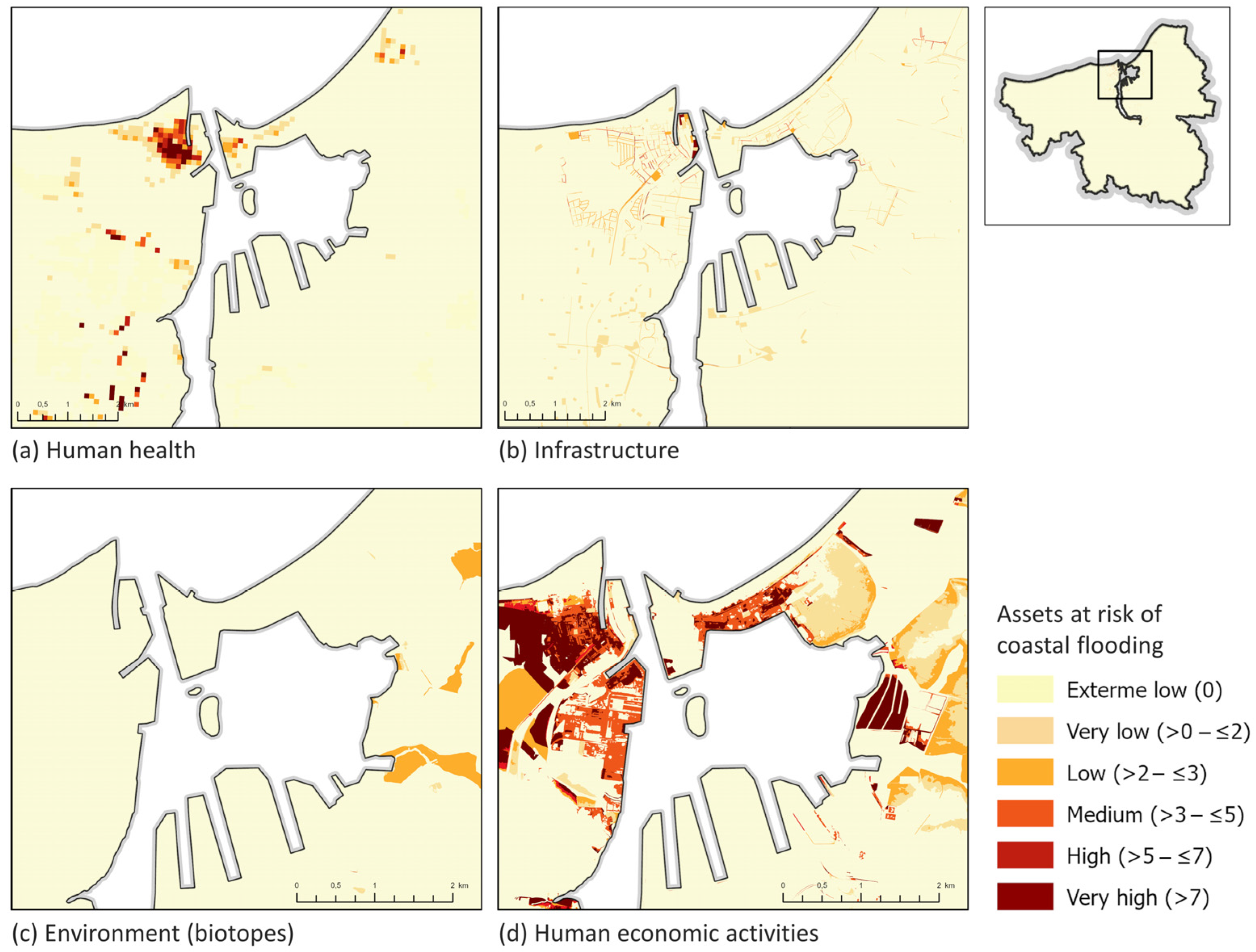
Coastal protection 1Expert estimatesExpert estimates-Coastal flood risk for the asset: human health, the environment, infrastructure and human economic activities (Index 0 to 5, dimensionless)--
1 Only mapped for the urban region of Rostock.
Table 3. Overview of the mapping outcomes. Method 1: Expert-based ES matrix approach, Method 2 = proxy indicators and data, Method 3 = InVEST models; Mapping outcome: yes = ES component could be mapped, yes * = ES component could be mapped, but not for the whole case-study region, no = ES component could not be mapped.
Expert-Based ES Matrix ApproachSimple GIS MappingInVEST Models
Ecosystem ServicesSupplyDemandSupplyDemandSupplyDemand
Food (from cultivated terrestrial plants)yesnoyesyesnono
Raw materials (from cultivated terrestrial plants)yesnoyesyesnono
Pollinationyesnonoyes *yesno
Local climate regulationyesnoyesyesyesyes *
Coastal protection 1yesnonoyes *nono
1 Only mapped for the Rostock urban region.
Table 4. Similarity values of the map comparison between the maps from expert estimates (expert-based ES matrix approach) and the indicators (A) green and blue area (%) (LULC data); (B) f-ETP-Index (literature data); (C) heat mitigation index (InVEST model Urban Cooling) in the urban region of Munich. Values: 0 indicates no similarity, and 1 very high similarity between the compared maps.
ABC
Local Climate Regulation Indicator Green and Blue Area (%)f-ETP-Index Heat Mitigation Index
Similarity indexMean0.630.910.69
Std. Dev.0.220.120.17
Disclaimer/Publisher’s Note: The statements, opinions and data contained in all publications are solely those of the individual author(s) and contributor(s) and not of MDPI and/or the editor(s). MDPI and/or the editor(s) disclaim responsibility for any injury to people or property resulting from any ideas, methods, instructions or products referred to in the content.

