Article

Modelling the Whole Profile Soil Organic Carbon Dynamics Considering Soil Redistribution under Future Climate Change and Landscape Projections over the Lower Hunter Valley, Australia

1
Sydney Institute of Agriculture, School of Life and Environmental Sciences, The University of Sydney, Sydney, NSW 2006, Australia
2
Landcare Research, Private Bag 11052, Manawatu Mail Centre, Palmerston North 4442, New Zealand
3
INRAE, UMR 1069, SAS, 65 Rue de Saint-Brieuc, F-35000 Rennes, France
4
UMR SAS, Institut Agro, INRAE, F-35000 Rennes, France
5
CSIRO Agriculture and Food, Black Mountain, Canberra, ACT 2601, Australia
*
Author to whom correspondence should be addressed.
Land 2023, 12(1), 255; https://doi.org/10.3390/land12010255
Submission received: 16 December 2022 / Revised: 9 January 2023 / Accepted: 12 January 2023 / Published: 14 January 2023

Abstract

:
Soil organic carbon (SOC) storage and redistribution across the landscape (through erosion and deposition) are linked to soil physicochemical properties and can affect soil quality. However, the spatial and temporal variability of soil erosion and SOC remains uncertain. Whether soil redistribution leads to SOC gains or losses continues to be hotly debated. These considerations cannot be modelled using conventional soil carbon models and digital soil mapping. This paper presents a coupled-model combining RothPC-1 which considers soil carbon (C) down to 1 m and a soil redistribution model. The soil redistribution component is based on a cellular automata technique using the multi-direction flow (FD8) algorithm. With the optimized input values based on land use, we simulated SOC changes upon soil profiles to 1 m across the Lower Hunter Valley area (11,300 ha) in New South Wales, Australia from the 1970s to 2016. Results were compared to field observations and showed that erosion was predicted mostly in upslope areas and deposition in low-lying areas. We further simulated SOC trends from 2017 until ~2045 in the area under three climate scenarios and five land use projections. The variation in the magnitude and direction of SOC change with different projections shows that the main factors influencing SOC changes considering soil redistribution are climate change which controlled the trend of SOC stocks, followed by land use change. Neglecting soil erosion in carbon models could lead to an overestimation of SOC stocks. This paper provides a framework for incorporating soil redistribution into the SOC dynamics modelling and also postulates the thinking that soil erosion is not just a removal process by surface runoff.

1. Introduction

The largest terrestrial pool of carbon (C) is found in soils [1], with approximately 2300 Gt (gigatons) to 1 m depth stored globally, 1550 Gt is an organic carbon and 750 Gt is an inorganic carbon, representing approximately three times the size of the atmospheric pool of C (760 Gt) [2,3,4]. Soil organic carbon (SOC) is linked to many soil physicochemical properties and is an indicator of soil quality [5,6]. SOC sequestration can be used as a mitigation strategy for human-induced greenhouse gas (GHG) emissions [7] by sequestering C from the atmosphere and transferring it into long-lived pools in soils [8,9,10]. Conversely, climate change may affect soil microbial activities, soil moisture and temperature regimes, leading to changes in SOC mineralization [11].
SOC storage in the landscape is mainly controlled by the C inputs (land use), decomposition, and soil redistribution [12]. Conversion from native vegetation to agricultural ecosystems, especially cropland, causes SOC depletion [13]. Conversely, the conversion from cropland into permanent grassland has been linked to increased SOC storage [14]. Soil redistribution (through erosion and deposition) by water and wind influences the spatial distribution of SOC by transferring C-enriched sediments laterally, burying some deeply in depositional areas downslope, or exporting them out of the catchment [15]. Wind erosion also causes dust emission and the removal of C- and nutrient-rich fine material (e.g., <22 μm) [16]. These redistribution types affect the flux and stock of SOC in the eroded or deposited soil particles [2,17,18]. Mineralization in the soil can be decreased during SOC depletion and accelerated by water disruption of soil aggregates or accelerated by degradation of macroaggregates due to wind erosion [19,20]. Contrarily, SOC concentrated in alluvial and colluvial sediments can decrease mineralization [2]. In the context of global change, the impact of whether soil redistribution leads to SOC gains or losses is hotly debated [21,22,23].
Understanding the fate of SOC under future scenarios has previously been modelled in selected areas using a coupled digital soil mapping (DSM) and simulation approach, with examples from Gray and Bishop [24], Meersmans, et al. [25] and Yigini and Panagos [26]. With these studies, a scorpan model [27,28,29] was first calibrated in an area using present-day or near-present-day observations. The projection of SOC storage into the future (forecasting) is then performed by modifying one or two of the model empirical factors (climate and land use) using the scorpan approach. This approach is quick and relatively simple to estimate SOC changes, however, it is empirical and has limitations compared with dynamic simulation models [30], and assumes an immediate equilibration between SOC and the changing factors. Moreover, these models do not explicitly have a time component and lack an underlying mechanism to model interactions between soil redistribution and SOC dynamics. While studies using soil C dynamic models such as Century and RothC have been applied to map soil C evolution (e.g., Cerri, et al. [31] and Falloon and Smith [32]), these models are one-dimensional single-layer models that only consider topsoil. These models do not simulate soil redistribution.
The aim of this study was to (a) evaluate the long-term impacts of soil redistribution on SOC dynamics, (b) simulate the SOC dynamics spatially and temporally via horizontal and vertical soil translocation and (c) quantify the impacts of changes in land use and climate on soil redistribution and SOC stock changes. This study presents a spatially explicit mechanistic model combining a modified SOC dynamics model and a soil redistribution component of water erosion. We apply this model to simulate SOC evolution over soil profiles of 1 m from 2017 until ~2045 across the Lower Hunter Valley, NSW, Australia to gain an understanding of the combined impact of soil redistribution, climate change and land use change on future SOC stocks.

2. Materials and Methods
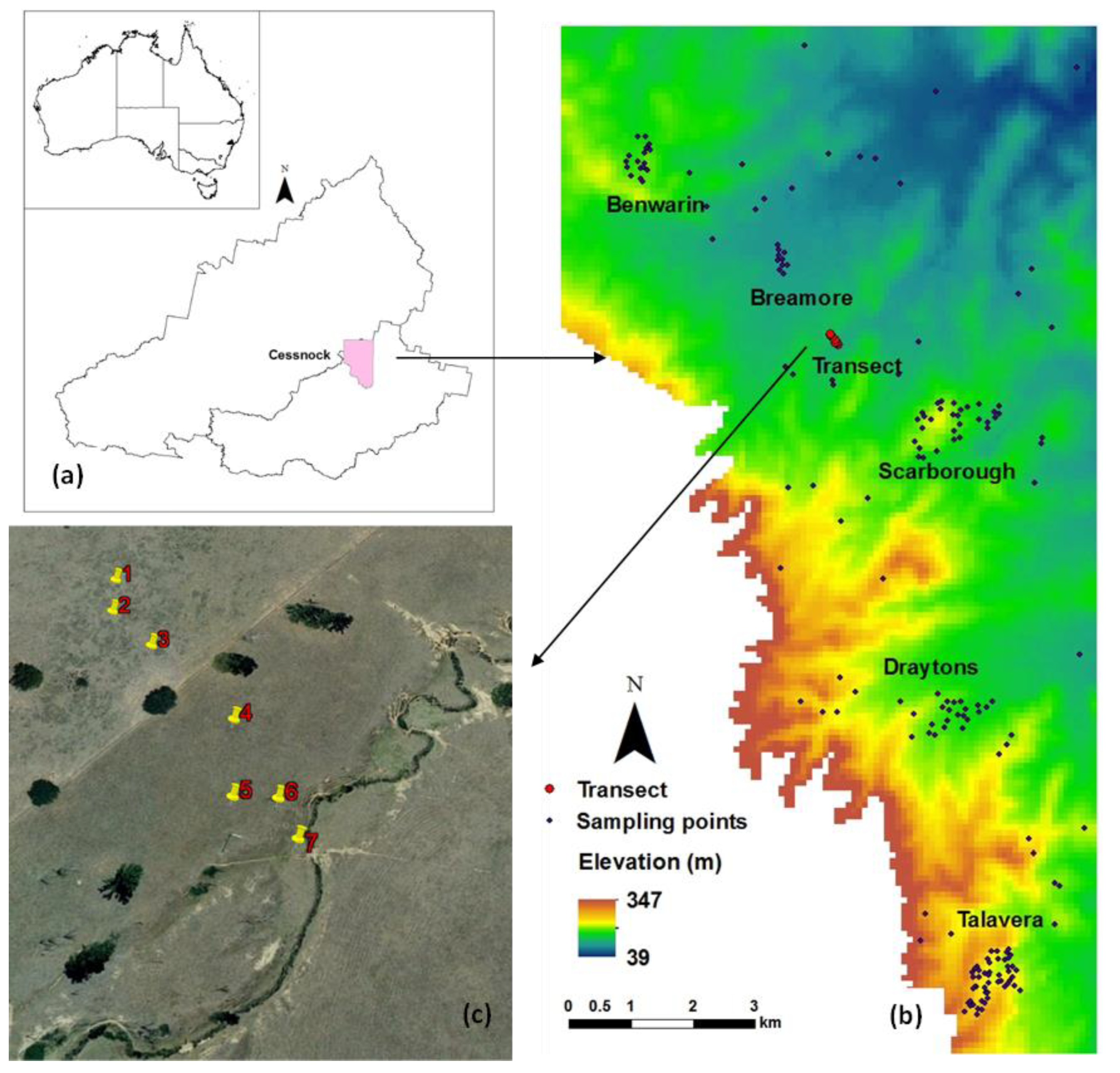
2.1. Study Site

The study area (151.23° E–151.32° E, 32.71° S–32.86° S) is in a sub-area of the HWCPID (Hunter Wine Country Private Irrigation District) in the Lower Hunter Valley, New South Wales, Australia, and covers a total area of about 11,300 ha (Figure 1a). It is a well-known wine production area where the first vineyard was constructed during the early 19th century [33]. This site is in the temperate climatic zone with warm humid summers and cooler humid winters. On average, this site receives over 750 mm of rainfall annually. This site area is situated in the Sydney Basin where the geology is predominantly characterized by Mesozoic sandstones and shales [34]. Topographically the study area consists of undulating hills, which rise to low mountains to the southwest. Elevation ranges from 39 m to 347 m (Figure 1b), with a mean elevation of 111 m and a mean slope of 5%. Viticulture industry is the major land use, followed by dryland agricultural grazing systems [35]. Dermosols, Calcarosols and Chromosols are the dominant soils types [36] which are equivalent to Acrisols, Calcisols and Lixisols/Luvisols according to WRB [37], or Alfisols according to the USDA Soil Taxonomy [38].

2.2. Soil Samples

The soil dataset we used contains 162 soil profiles. Soil samples were collected from different depths from several surveys [39,40,41] including a whole-area survey and detailed field-scale surveys in five vineyards: Benwarin (mean elevation: 115 m; mean slope: 4%), Breamore (74 m; 1%), Draytons (118 m; 4%), Scarborough (107 m; 6%) and Talavera (152 m; 9%) (Figure 1b). Mass preserving soil profile splines [42] were fitted to each profile data individually to obtain soil carbon concentration at standardized depth intervals: 0 to 5, 5 to 15, 15 to 30, 30 to 60, and 60 to 100 cm.
The soil samples were air-dried at room temperature (20–22 °C), removed stones/gravels and debris and then sieved to pass a 2 mm sieve. A portion of the soil sample (about 100 g) was ground in an agate grinder and sieved through a 100-mesh sieve (0.149 mm). SOC concentration of the samples was determined using the dry combustion method.
Soil texture (clay content) was needed to predict changes in SOC in the coupled model. We utilized a spectral modelling approach to supplement our observations. Soil samples were scanned with a portable visible-near infrared (vis-NIR) spectrophotometer, ASD (Analytical Spectral Devices, Boulder Colorado) Agrispec, from 500 to 2500 nm with a Spectralon® white tile as a reference reflectance. Clay (<2 μm), silt (2–20 μm), and sand (20–2000 μm) were predicted from the spectra based on a spectral library of soils from different locations in New South Wales, Australia [43,44,45].
To understand the contribution of soil redistribution on SOC content, we used data from a transect in a vineyard (Figure 1c): from the hill crest and down to the gully. Seven soil cores were collected approximately 40 m apart, and for each soil profile, soil horizons were identified visually. SOC was measured using a vis-NIR spectrometer at 10 cm intervals down to 1 m depth and predicted from the spectra of the SOC data in Hunter Valley. The vis-NIR calibration model was locally fitted and had good agreement with the SOC observations.

2.3. Coupled Model

A SOC dynamics model and a soil redistribution model were combined to model the impact of soil redistribution on SOC transfers. The coupled model was run at a 90-m spatial resolution.

2.3.1. SOC Dynamics Model

The SOC dynamics were modelled based on the RothPC-1 (the PC standing for profile C) model [46] and written in the R statistical software [47]. RothPC-1 is based on the earlier topsoil model RothC-26.3 [48] and models the turnover of organic C in the top meter of soil, with two extra parameters, p which moves organic C down the profile by an advective process and s which slows decomposition with depth. RothPC-1 was run on a monthly time step. The SOC stocks and C inputs are partitioned into five conceptual compartments: decomposable plant material (DPM), resistant plant material (RPM), microbial biomass (BIO), humified organic matter (HUM) and inert organic matter (IOM). As this area did not have detailed SOC fraction measurements, we only modelled total SOC by initializing the model with five compartments starting from 0. Soil profiles were divided into 0–30, 30–60 and 60–100 cm layers. SOC stocks were calculated based on SOC concentration and bulk density. Bulk density (g cm−3) was predicted using the PTF of Adams [49] which is a function of mineral bulk density and soil organic matter (SOM) content.
ρ b = 100 O M % ρ O M + 100 O M % ρ m
where ρb is soil bulk density, ρOM is organic matter bulk density (0.224 g cm−3), ρm is mineral bulk density, and OM% is the percentage of organic matter. The mineral component is based on local data. This PTF allows bulk density to change with the change in SOM and all the simulations and results in this study using this PTF were acceptable.

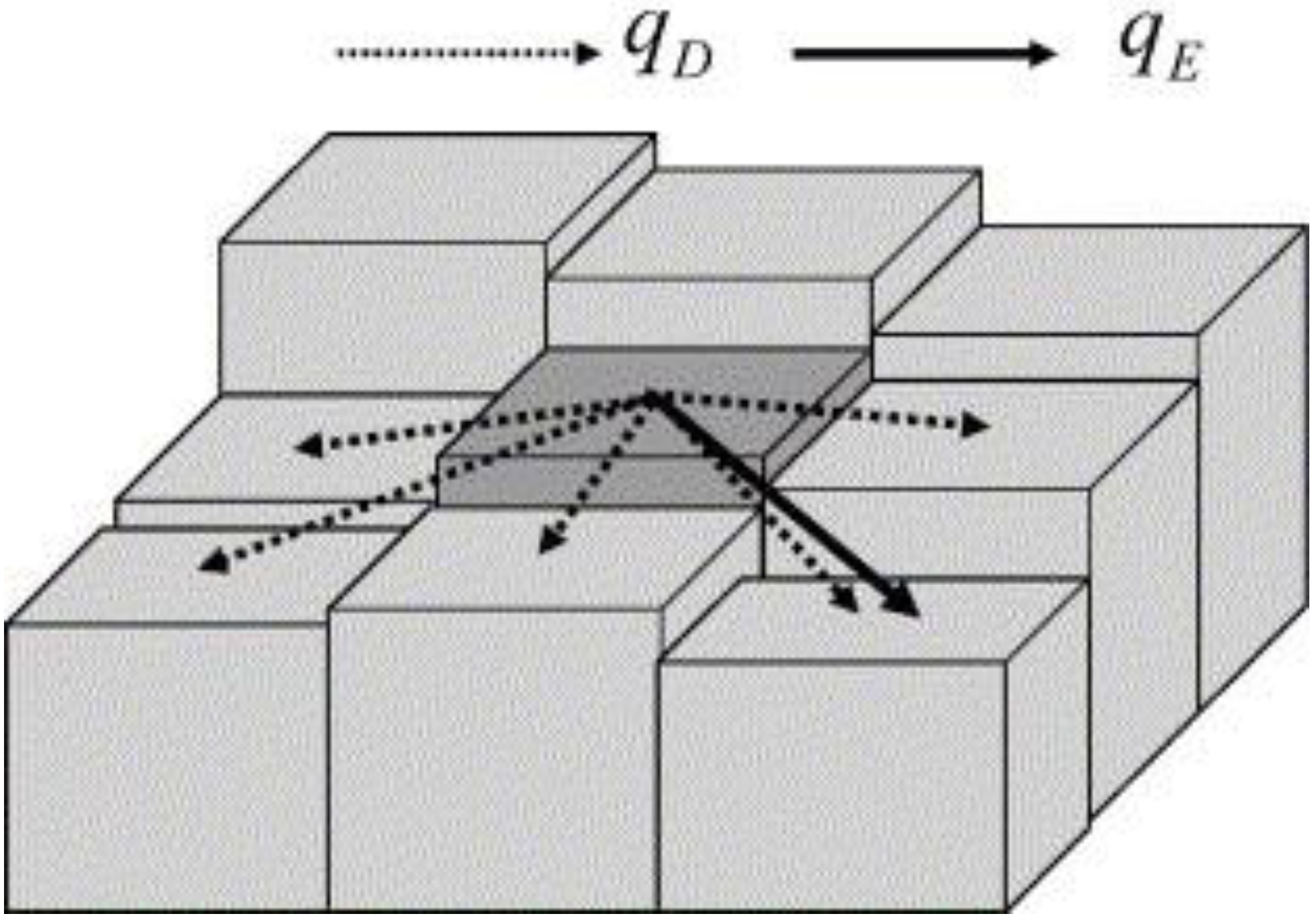
2.3.2. Soil Redistribution Module

Soil redistribution is the translocation of soil material due to erosion or deposition by water, wind or tillage in a specific location. In this study, only water erosion was considered. The soil redistribution model simulates water erosion based on rainfall events that could redistribute soil. Soil redistribution is estimated by:
Ec = 1000α × β × S × (P − E)
where Ec (in meters) is the change in elevation, S is slope, P is annual precipitation (in millimeters), E is annual evaporation (in millimeters), α is a constant determining soil erosion and varies for different land uses, and β is a constant to modify soil erosion rate by SOC content as soil erosion susceptibility has been shown to depend on SOC content [50]. One advantage of the soil redistribution model is that it provides feedback between erosion rate distribution and land use and SOC content change through the adjustment of α and β. Runoff is predicted only when P − E > 0 and soil is moved from a specific cell to eight adjacent cells that were lower than the eroding cell based on a cellular automata technique using the multi-direction flow (FD8) algorithm [51,52], as shown in Figure 2 (from [53]).
  • The updated elevation, subtracted from the previous one and EC was entered into the SOC dynamics model. If soil erosion or deposition was predicted, soil layer boundaries were updated to include the addition or removal (Figure 3). SOC concentration of the deposited soil to a given cell was assumed to have the same content as that from the eroded soil. At the end of the simulation, three areas were identified: stable (−1 cm < change in soil depth < 1 cm), net soil erosion (change in soil depth ≤ −1 cm), and deposition (change in soil depth ≥ 1 cm). The combined modelling analysis was programmed in the R language.

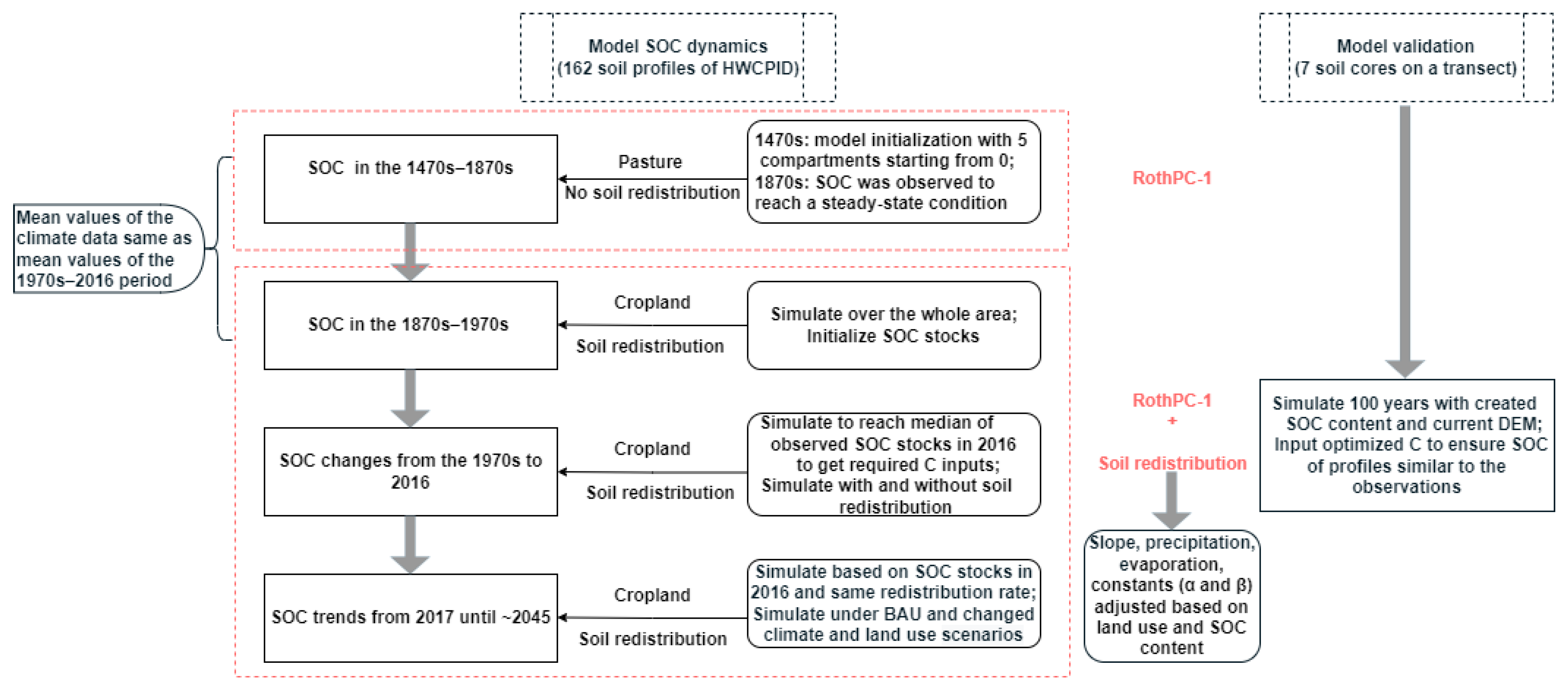
2.3.3. Model Settings

For the initialization of the coupled model, C pool sizes were obtained by running the model until it reached a steady-state condition. The simulation period was divided into four stages:
  • The 1470s–1870s. The model simulated SOC dynamics for 400 years until the 1870s when SOC was a steady-state condition. During this simulation period, land use was assumed to be pasture without consideration of soil redistribution.
  • The 1870s–1970s. Pasture was changed to cropland. The model simulated the change in SOC with time under cropland conditions.
  • The 1970s–2016. The model was run for the 1970s–2016 period repeatedly using a Markov Chain Monte Carlo (MCMC) sampling method [54] with different plant residue inputs and erosion rates for different land uses to get the required C inputs to reach median values of observed SOC stocks in the 0–30 cm layer in 2016 for five vineyards. Latin hypercube sampling (LHS) [55], a stratified-random procedure to cover full range of each variable by maximally stratifying the marginal distribution, was used to replicate the distribution of C inputs to get the representative inputs for the entire study area. To estimate the effect of soil redistribution on SOC stock changes, the model simulated SOC under two approaches: with and without soil redistribution. The fits of measured and modelled SOC stocks in the 0–30 cm soil layer in 2016 for the entire study area under two conditions are shown in Figure S1.
  • 2017–2045. The model simulated SOC stocks from 2017 to 2045 under different climate and landscape scenarios.
To validate the coupled model, a separate simulation was conducted. The model was run over 100 years to simulate soil evolution along the transect with the SOC content datasets down the profile using the current DEM as input data. We ran the model with optimized C inputs to ensure that the SOC distribution down the profiles reached similar conditions as the observations. Figure 4 shows the flowchart for model simulation and model validation.

2.3.4. Input Data for the Coupled Model

Climate data (monthly precipitation, open-pan evaporation and mean air temperature), soil properties (initial SOC stocks, clay content, root distribution in the soil profile, drainage conditions and bulk density), management (annual C inputs from plant residues, changing land use during the simulation, residue management), soil redistribution data (initial elevation and constants (α and β)) were used as inputs to the model (Table 1). No manure addition and export of crop residues were considered in this study.

Climate Data

For the 1970s–2016 period, the climate data were derived from the Australia-wide climate grids from the Australian Bureau of Meteorology. Mean values of the current climate were used to represent the mean values over the 1470s–1870s and 1870s–1970s periods. Two projected climate datasets over the 2017–2045 simulation period were obtained from the Australian climate change projections by CSIRO and Bureau of Meteorology. These projections were described by the mean of different models, as will be discussed in Section 2.5.

Soil Data

Table S1 shows the percentiles (10th, 50th and 90th) for observed SOC stocks in 2016 in five fields and the entire study area. Soils in Benwarin, Scarborough and Talavera have larger SOC stocks than those in Breamore and Draytons in the 0–30 cm layer. SOC stocks in Benwarin, Draytons, Scarborough and Talavera are larger than those in Breamore in the 30–60 and 60–100 cm layers. Observed SOC stocks within the entire study area range from 28.4 to 94.5, 9.6 to 49.2 and 5.6 to 35.1 t C ha−1, respectively, in the 0–30, 30–60 and 60–100 cm soil layers (median = 55.7, 22.8 and 18.5 t C ha−1).
Clay content (%) during the whole simulation period was based on a digital soil map of the area and assumed to be constant over time [56].

Land Use Data

Four different land uses (forest, natural grassland, grassland and cropland) were considered in this study area. For the pasture (the 1470s–1870s) and cropland (1870s–1970s) stages, annual plant residue inputs were set at 10 and 4 t C ha−1, respectively. For the 1970s–2016 period, required C inputs to the soil to maintain the 2016 SOC level for five fields were obtained by repeated simulations using the MCMC sampling method. Rainfall influences crop yield, thus the impact of rainfall on C inputs was considered in this study. Annual rainfall in a specific year divided by the long-term average annual rainfall was used as a constant to adjust C inputs. We used the same values for the C inputs from the natural grassland and grassland residues for the five fields. Based on LHS, the representative C inputs for the entire study area were set at 12.5, 6.1, 6.4 and 3.0 t C ha−1 yr−1 for the forest, natural grassland, grassland and cropland (Table 2).

Soil Redistribution Data

Historical precipitation and evaporation data within the study area were used to get a realistic soil redistribution rate. Since croplands are the most vulnerable to erosion because of the sparse vegetation cover compared to forests and grasslands [57], α (from Equation (2)) was set at values of 0.0125, 0.015, 0.015 and 0.02 for the forest, natural grassland, grassland and cropland. As SOC increases, soil erosion is expected to decrease, β was set at 0.25 for C content between 1 and 2% and 0.05 for C content higher than 2% in the 0–30 cm layer. α and β were determined according to the data of Montgomery [58] with erosion rate distributions for native vegetation and agriculture lands.
Soil redistribution is considered as the absolute value of soil displaced due to erosion and deposition. Net soil deposition is presented as a positive rate of soil redistribution, whereas net soil erosion is presented in negative values. Two indicators were computed: cumulative soil redistribution rate over the study area and percentage of area with soil erosion or deposition.

2.4. Digital Soil Maps

To assess the performance of the coupled model, we compared its simulation with the prediction of SOC stocks using the Cubist regression model and observed SOC data. Root mean square error (RMSE) was used to assess the performance of the models.
Cubist [59], a rule-based regression tree model, is quite effective within the digital soil mapping community [27,39,60,61]. The algorithm partitions the observed data and creates a set of “if-then” rules for each subset. Each rule represents a multivariate linear model of the predictor [62]. We fitted 100 Cubist models using random samples with replacement in R to extract the mean prediction of SOC stocks. The Cubist algorithm has three parameters: rules, committees and extrapolations. In this study, we used five rules to partition the data, 5% of data extrapolations to constrain model features, and 10 committees which mean 10 boosting iterations to obtain a prediction.
A suite of environmental variables were considered: Landsat 7 with the enhanced thematic mapper plus (ETM+), normalized difference vegetation index (NDVI), DEM and terrain attributes derived from the DEM: slope, topographic wetness index (TWI), terrain ruggedness index (TRI), multiresolution ridge top flatness (MrRTF), aspect, multiresolution index of valley bottom flatness (MrVBF), terrain position index (TPI), relative slope position (RSP), slope length and steepness factor (LS-factor) and valley depth. All covariates were at 90-m resolution.

2.5. Scenario Design

Multiple scenarios were conducted forecasting future SOC evolution over the simulation period (2017–2045) by considering two factors: climate (described by three scenarios) and landscape (described by five scenarios).

2.5.1. Climate Changes

Three climate scenarios were conducted: business-as-usual (BAU) climate and two projected climates. BAU was considered as same as the climate in 2016. The projected climate changes for the 2017–2045 period were predicted using eight global climate models (Table S2) from the 40 CMIP5 (Coupled Model Intercomparison Project Phase 5) models considering model skill and model genealogy. Each model was forced by two RCPs (Representative Concentration Pathways): RCP 4.5 and RCP 8.5. The means of models with RCP4.5 and models with RCP 8.5 were considered as the two projected scenarios.
RCP4.5: CO2 concentrations are slightly above 660 ppm until after mid-century, but emissions peak earlier (around 2040), and the CO2 concentration reaches 540 ppm by 2100.
RCP8.5: a future with little curbing of emissions, with a CO2 concentration continuing to rise rapidly, reaching 940 ppm by 2100 [63].
For the BAU and climate change scenarios, the average monthly temperature is similar, however, the projection of monthly mean rainfall is lower than that of BAU (Table S3).

2.5.2. Landscape Scenarios

Land use was projected using Landsat 5, 7 and 8 Surface Reflectance Tier 1 data and MODIS Land Cover Type product (MCD12Q1) on Google Earth Engine (GEE) [64] cloud computing platform. The MODIS data provides global land cover maps at 500-m spatial resolution at annual time steps from 2001 through 2013. Different Landsat data were used for different periods: Landsat 5 for years before 1999 and 2003–2011, Landsat 7 for the years 2000–2002 and 2012 and Landsat 8 for years 2013–2016. To avoid the effect of the stripes of Landsat 7, we mainly used Landsat 5 and 8. However, the data for 2000–2002 and 2012 were incomplete due to the cloud and cloud shadow of Landsat 5, so we used partial Landsat 7 as a supplement.
A total of 943 sampling points with a 500-m grid spacing were derived as representative pixels from MODIS data across the study area, thus the land cover information from 2001–2013 could be obtained. Seventy (70) % of the pixels were used as training data. After masking cloud and cloud shadow for Landsat data, 13 prediction models were built based on the land cover information and the Landsat data for training points for each year during 2001–2013. By using the mode function for the 13 models, a final model related land cover and Landsat can be built and then the historical land use prediction from the 1970s to 2016 was obtained.
Based on the MODIS product, from 2001 to 2013, cropland in the area increased by 13–91% and the natural grassland increased by 10–90%. Five contrasting landscape scenarios in the study area for the 2017–2045 period were designed using a cellular automata technique in Python:
  • baseline corresponding to land use in 2016,
  • maximum area increases in cropland (MaxC) (91%),
  • minimum area increases in cropland (MinC) (13%),
  • maximum area increases in grassland (90%) (MaxG), and
  • minimum area increases in grassland (MinG) (10%).
These scenarios were used to simulate SOC stocks under extreme conditions.

3. Results

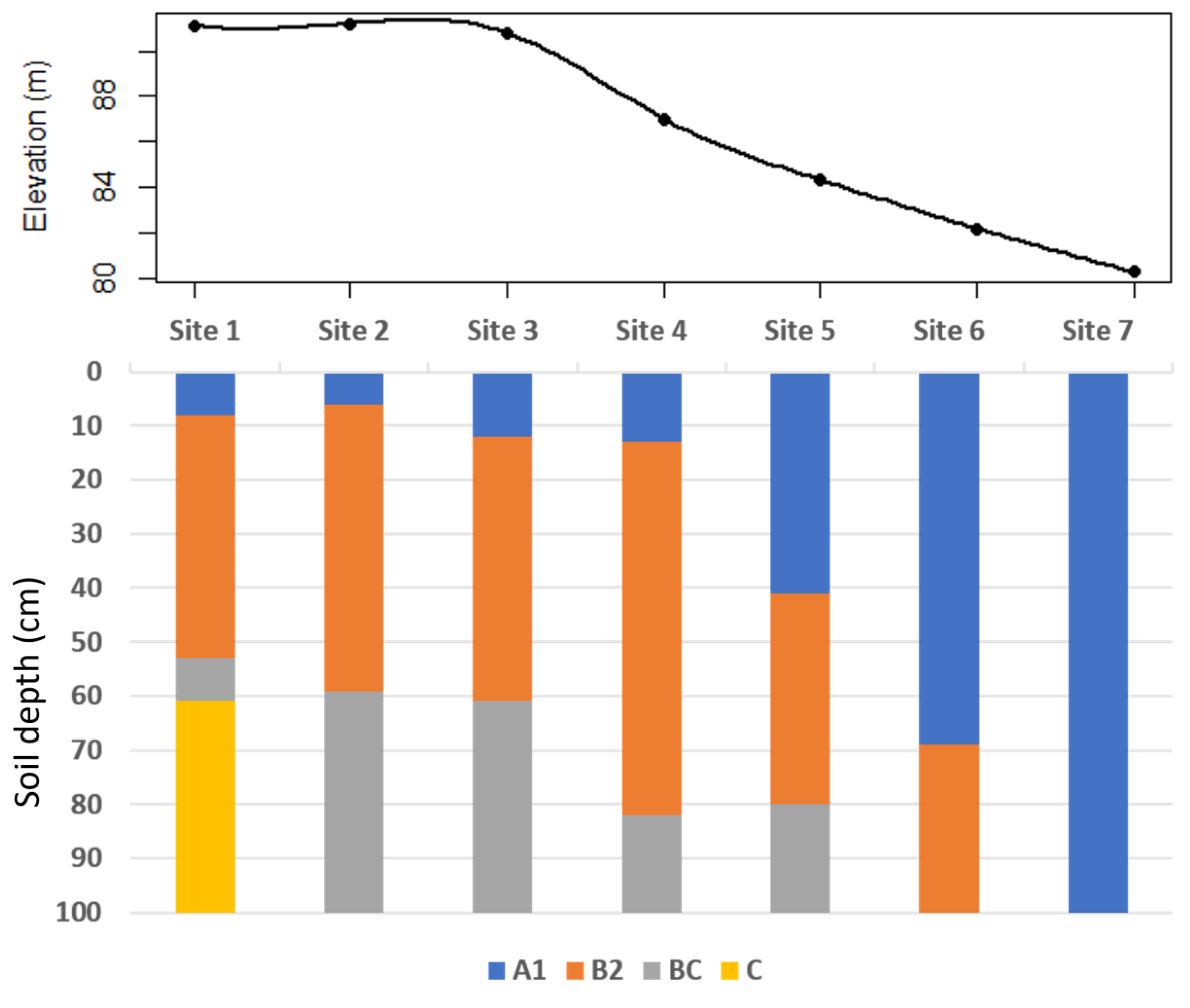
3.1. Validation of the Model with the Transect Data

To evaluate the performance of the coupled model, simulations of SOC evolution over 100 years along a transect were compared with field observations. The transect was from the top of the hill to the bottom, where a large amount of soil erosion was observed. Figure 5 shows the location and soil horizon distribution of current soil profiles across the transect. Clearly, the A1 horizon increased from site 1 to site 7, which shows that the A1 horizon from the top of the hill had been severely eroded and deposition has occurred downslope. At site 7 near the gully, more than 1 m of A1 horizon was observed. The field observations of SOC of three profiles (site 2 (top of the hill), site 4 (middle) and site 7 (bottom) (Figure S2) were taken as comparisons. It shows that SOC stocks are high in topsoil and decrease with depth. For profiles on the top and middle of the hill, SOC stocks are lower than that of the profile at the bottom.
Figure S3 shows the elevation change of the transect over 100 years. The thickening of the profile (site 7) was observed at the bottom of the hill and the thinning of the soil profile (site 3 and 4) at the top of the hill. The model can also simulate the trend in SOC by comparing the simulations of three profiles (site 2, site 4 and site 7) with field observations (Figure S4). It indicates that SOC at top and middle of the hill has been eroded, then SOC is enriched at the bottom. Especially for site 4, more than half of the profile has been eroded. This analysis demonstrated that the coupled model is able to simulate soil erosion and soil C redistribution as observed in the landscape.

3.2. Soil Redistribution and Its Impact on SOC

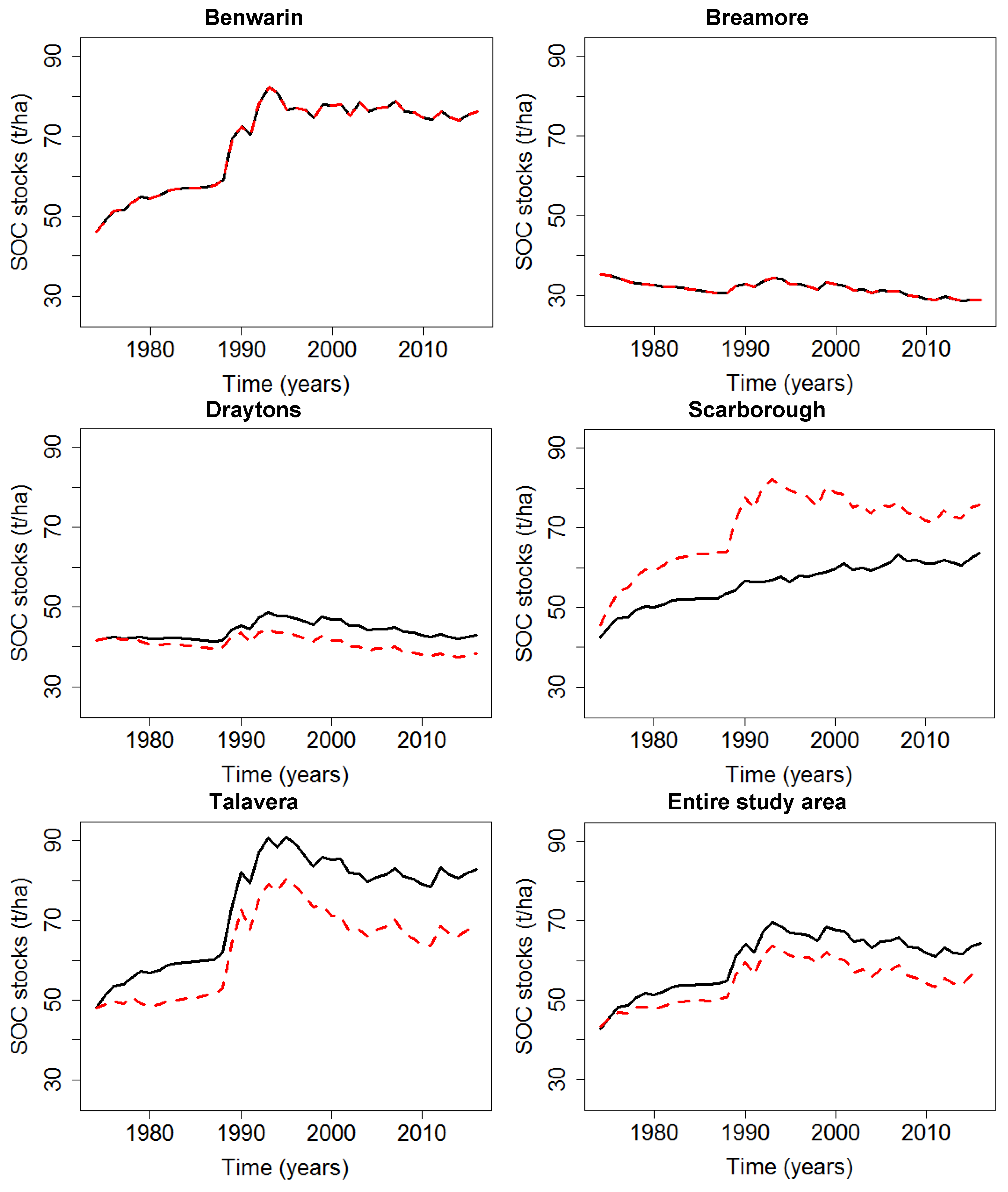
3.2.1. The Effect of Soil Redistribution

We first ran the models over the whole area from the 1870s to 1970s to initialize the SOC stocks. We then simulated the evolution of SOC from the 1970s to 2016 with and without considering soil redistribution over five farms and the whole area. Over this simulation period, soil erosion appears to have a large influence on SOC stock in Draytons and Talavera: mean soil redistribution rate was −0.11 and −0.35 t ha−1 yr−1. Soil deposition dominated in Scarborough with a mean soil redistribution rate of 0.28 t ha−1 yr−1. This is because these vineyards are located in the area of the Hunter Valley that has undulating and complex relief. The mean soil redistribution rate was zero in Benwarin and Breamore since these vineyards are found in a relatively flat area of the Hunter Valley (Table 3).
Soil erosion prevailed over soil deposition in the study area (Table 3): a mean soil redistribution was estimated at a rate of −0.18 t ha−1 yr−1. The soil redistribution rates were comparable with those predicted by Bui, et al. [65] with an estimated tolerable soil loss of 0.2–0.4 t ha−1 yr−1 by assuming a bulk density of 1.3 Mg m−3 and an average soil production rate of 1.5 × 10⁻⁵ m yr−1 uniformly over Australia.
Considering areas with soil thickness change >1 cm, net soil erosion areas were 2.2% of the entire study area which had a mean erosion rate of −0.57 t ha−1 yr−1, while areas experiencing net soil deposition were 3.5%: mean deposition rate was 0.06 t ha−1 yr−1 (Figure S5).
Overall, the net soil erosion resulting from water processes was associated with slope gradient. Steep, high-elevation slopes (uphill) induced more soil erosion than low-elevation, gentle slopes (downhill). For example, the largest net soil erosion rate was predicted in Talavera where the mean slope (9%) was highest, thus the mean SOC stocks strongly fluctuated. The results agreed with Zingg [66] who first described mathematically the effects of slope steepness and slope length on field soil erosion.

3.2.2. SOC Dynamics

At Draytons and Talavera, soil redistribution processes caused mean SOC stocks in 2016 to decrease compared to simulation with no redistribution from 37.8 to 34.0 and 74.9 to 61.8 t C ha−1 in the 0–30 cm layer. The decrease also affected the whole profile from 42.9 to 38.3 and 82.8 to 67.6 t C ha−1 in the 0–100 cm. There was little soil loss in Breamore and Benwarin areas. SOC stock change by redistribution was dominant in Scarborough which had a mean slope of 6%: SOC stocks increased from 56.8 to 68.4 and 63.6 to 75.8 t C ha−1 in the 0–30 and 0–100 cm layers, respectively.
Over the entire study area, mean SOC stocks due to soil redistribution decreased from 57.9 to 52.0 t C ha−1 in the 0–30 cm soil layer and 64.4 to 56.6 t C ha−1 in the 0–100 cm soil profile (Table 4, Figure 6). Soil redistribution lowered SOC stocks in net erosion areas (249 ha) with a mean of 24.5 t C ha−1 and increased in net deposition areas (396 ha) with a mean of 31.1 t C ha−1 in the 0–100 cm soil layer.
In this study, soil redistribution induced SOC loss for the entire study area which agreed with the study of Lal and Pimentel [22] and Lacoste, et al. [67], but not with Van Oost, et al. [22]. The loss or storage of soil due to soil redistribution depends on the exportation or burial of the eroded particles, the increase or decrease in C mineralization dynamics and the model assumptions [68].

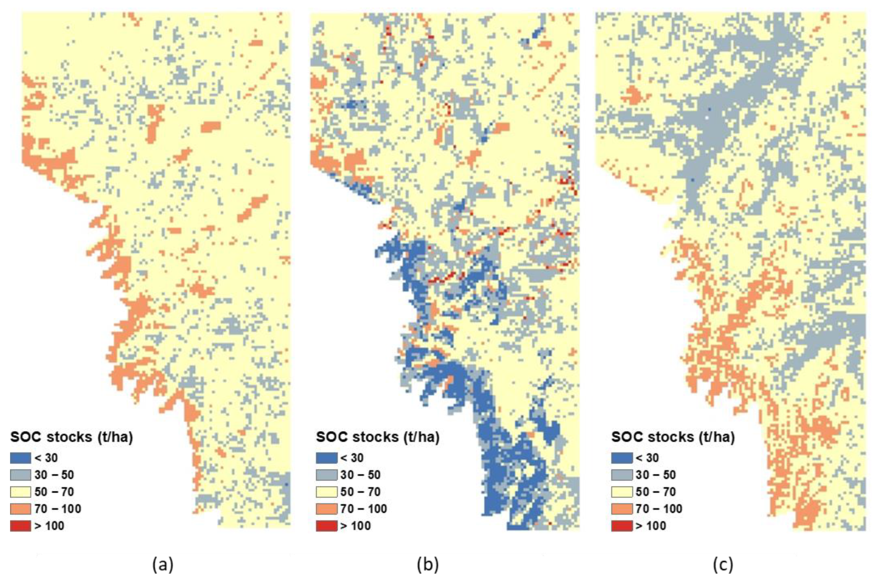
3.2.3. Spatial Distribution of SOC Stocks

Figure 7 shows that the spatial distribution of SOC stocks over the entire study area was closely associated with that of soil redistribution. The mean SOC stocks were 57.9, 52.0 and 56.8 t C ha−1 across the study area estimated by the model without soil redistribution (Figure 7a), associated with soil redistribution (Figure 7b) and Cubist regression model (Figure 7c). Compared to the field observations (mean SOC stock of 55.7 t C ha−1), the RMSE were 28.28, 37.19 and 21.74 t C ha−1. Clearly, the spatial patterns of SOC stocks in 2016 by three models were similar in the northern and eastern areas, while opposite patterns were found in the mountainous region in the southwest.
In the mountainous region in the southwest, SOC stocks were large (70–100 t C ha−1) based on the model without soil redistribution and Cubist regression model but low (0–30 t C ha−1) for the model that considered soil redistribution. The models with no redistribution assume the only production of biomass from forests in the mountainous region produced high SOC. On the other hand, at hillslopes, a prominent effect of water erosion redistributed more soil compared to the plains, deposited or exported those soils out of the study area, thus soil erosion was larger than soil deposition, decreasing SOC stocks. As there is a lack of samples on the steep slopes, we cannot verify the actual SOC content. The DSM model predicts a high C stock in those areas as it relates to higher elevation. The model associated with soil redistribution should be considered in future studies, especially the study sites with the mountainous area which is difficult to achieve with an empirical model.

3.3. Future Simulation

To observe the factors influencing soil evolution, the coupled model simulated SOC dynamics until ~2045 based on SOC stocks in 2016 and the same soil redistribution rate for the entire study area under contrasting situations: (1) BAU climate and changed landscape, and (2) changed climate and BAU landscape.

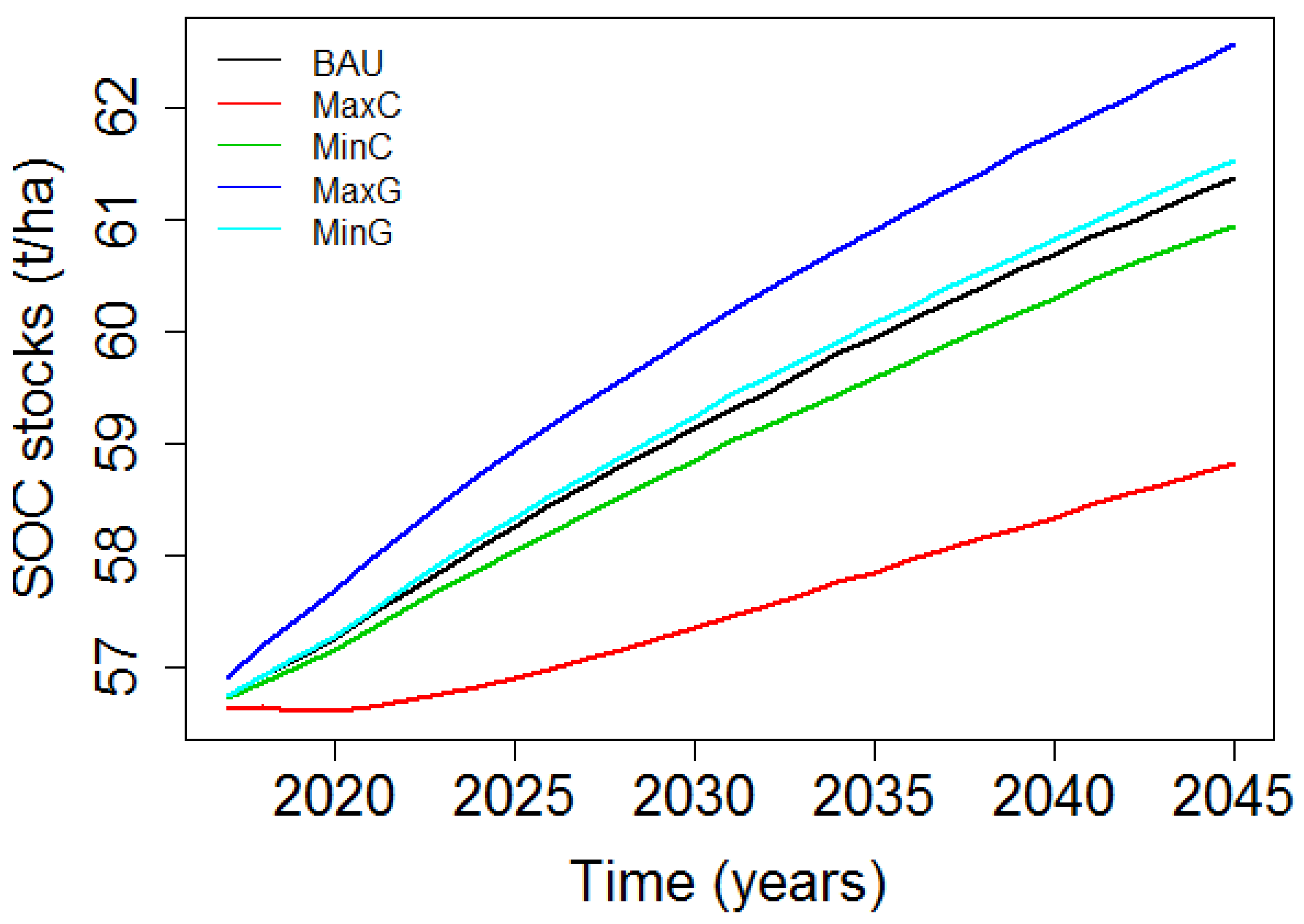
3.3.1. The Impact of Land Use

SOC stocks were simulated from 2017 to 2045 under BAU climate and different landscape scenarios. Generally, marked variations in SOC stocks were demonstrated with contrasting landscapes (Figure 8). Compared with the BAU scenario, MaxC had the greatest change in SOC stocks (−2.5 t C ha−1) followed by MaxG (+1.2 t C ha−1), MinC (−0.4 t C ha−1) and MinG (+0.1 t C ha−1). This indicates that land use resulted in different C inputs influencing SOC dynamics. This is consistent with the study by Don, Scholten and Schulze [14] where the land use conversion from cropland to grassland induced SOC storage.

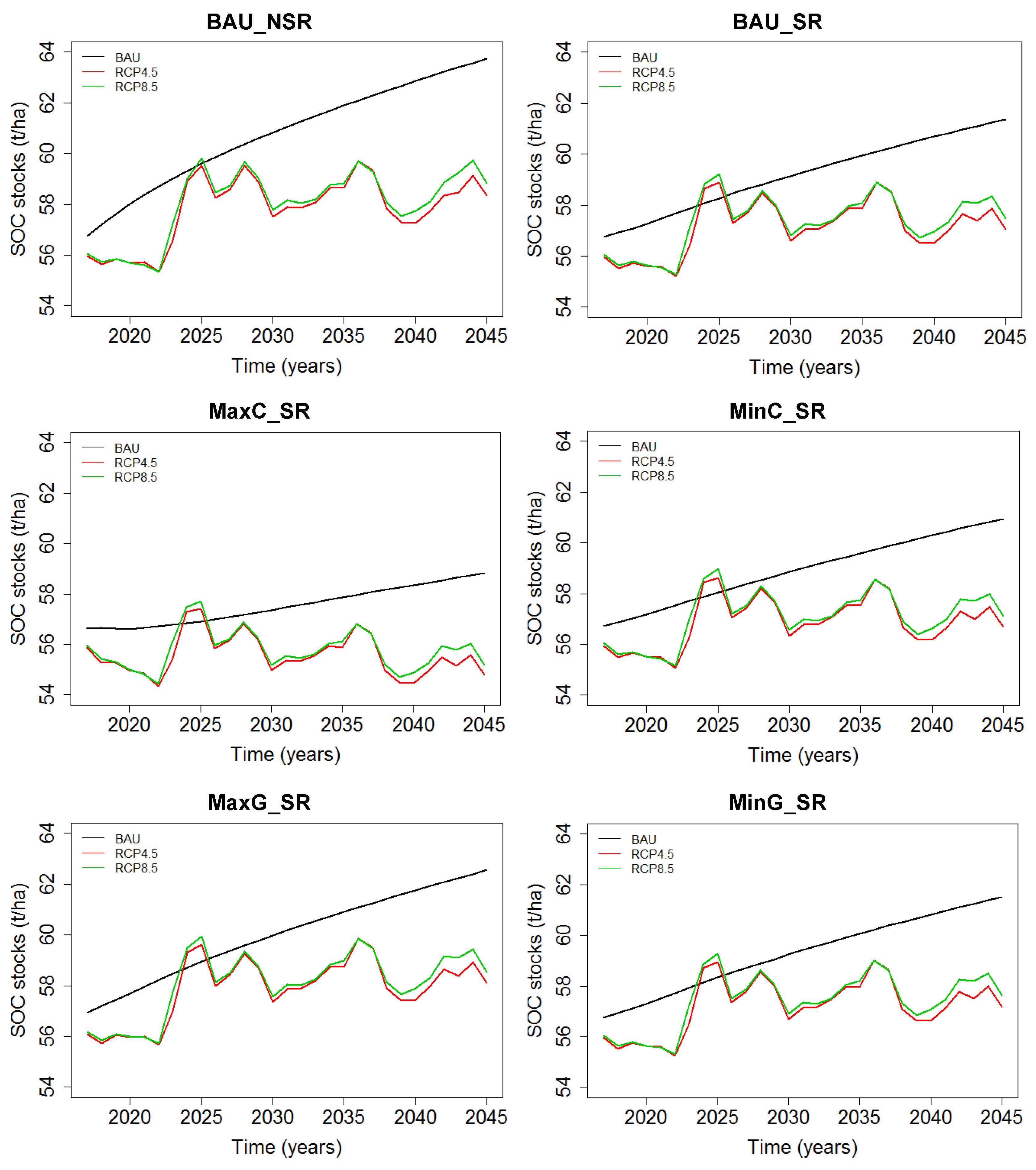
3.3.2. The Impact of Climate Change

Two projected climate scenarios decreased SOC stocks compared with BAU climate under all landscape scenarios, in agreement with the studies which estimated a decline of SOC storage under climate change at the landscape scale [67], the continental scale [69] or the global scale [70]. As the mean monthly temperature between the BAU and climate change scenarios was similar (Table S3), thus the C mineralization rate resulting from temperature was not the main influencing factor on SOC dynamics. The lower precipitation caused a change in crop yield and then decreased SOC stocks. The effect of climate change on SOC is still debated as they probably affect C mineralization and plant productivity [71]. According to Lacoste, Viaud, Michot and Walter [17], SOC storage increased by considering the indirect impacts of climate change on crop yields and plant photosynthesis. It was not the situation in this study as C input was constant and the impact of climate change on biomass production was not considered.
Under BAU landscape, SOC stocks decreased with soil redistribution (BAU_SR) compared to the one without soil redistribution (BAU_NSR). This could lead to over-estimate of SOC stocks if soil erosion is not considered for future scenarios. Considering the soil redistribution situation, generally, SOC stocks for the 0–100 cm layer decreased in RCP 4.5 and RCP 8.5 scenarios compared to BAU climate under all landscape scenarios. Mean decreases in SOC stocks were −4.3, −4.0, −4.3, −4.5, −4.3 t C ha−1 under BAU, MaxC, MinC, MaxG and MinG landscape scenarios with RCP 4.5 and −3.9, −3.6, −3.8, −4.0, −3.9 t C ha−1 under BAU, MaxC, MinC, MaxG and MinG with RCP 8.5 (Figure 9). The magnitude of mean SOC loss between different landscape scenarios for RCP 4.5 and RCP 8.5 was similar. The five landscapes had differing sensitivities to RCP 4.5 and RCP 8.5, but the difference was slight, ranging from −0.4 to −0.6 t C ha−1. These results indicated that the primary factor influencing SOC dynamics was climate change which controlled the trend of SOC stocks, followed by land use change.

4. Discussion

Previously, two models have been established to examine the interaction between soil redistribution and carbon fluxes on agricultural land: SPEROS-C which integrates a spatially distributed water and tillage erosion model (SPEROS) [72,73] with a carbon dynamics model, based on the introductory carbon balance model (ICBM) [74], and a modelling approach which links a spatially explicit SOC dynamics model (adapted from RothC-26.3) with a soil-redistribution model (LandSoil) [17]. Comparing with these two models, our coupled model has the advantage that it provides feedback between erosion rate distribution and land use and SOC content change through the adjustment of constants to predict soil evolution by considering two major processes of the complex soil systems in a spatially explicit way at the landscape scale. Our coupled model presented a smaller but comparable mean soil erosion rate of 0.57 t ha−1 yr−1 with the predictions by SPEROS-C (0.71 t ha−1 yr−1) and LandSoil coupled with adapted RothC-26.3 (3.95 t ha−1 yr−1).
This model could represent all climate changes and multiple land uses and their impacts on the spatial variability of soil. This approach is a useful tool to better understand soil functioning and support landscape management decisions and provides new thinking that soil erosion is not just a removal process by surface runoff, such as developed in the Revised Universal Soil Loss Equation (RUSLE) [75].
The approach also had uncertainties and limitations due to assumptions and the lack of validation data. For example, only soil redistribution by water is considered and no-tillage erosion is explicitly modelled. Rill or interrill water erosion was not discussed. The rainfall even-based soil redistribution was estimated according to rainfall, evaporation and slope, without considering the influence of soil surface characteristics (crusting, roughness), soil particle size, sediment concentration in the runoff, soil saturation, and soil infiltration. We used two constants (α and β) to modify the erosion rate of different land use and SOC content, however, we lack data to validate the different erosion rates. On the other hand, we ran the RothPC-1 model for 400 years with mean values of the climate for the 1970s–2016 period to represent the historical climate data and initialized five conceptual pools starting from 0. In addition, a large-scale spectral library was used to predict the clay content of the HWCPID soil profile sample, and a local calibration model for predicting the SOC of the transect data. We only used a dataset of seven cores along a transect to validate the coupled model. Even though the coupled model shows the change in elevation and the thickening of the profile at the bottom of the hill and the thinning of the soil profile at the top of the hill, we do not have a detailed analysis of soil profiles to validate the coupled model. In terms of the C input to the soil, we got the required C inputs to ensure the simulations reached to median values of observations using MCMC and got the representative C inputs for the entire study area using LHS, but we lack validation data to solve the C input constraint. For future scenarios, the impact of climate change on biomass production was not considered, the landscape scenarios we used are rudimentary, and the climate change scenarios do not have external forcings and feedback.
As a ‘light coupling” model by coupling two separate models, several improvements should be focused on: (i) further accurately examine initial SOC stocks and C inputs which impact mostly the prediction; (ii) consider another significant soil erosion process (tillage erosion) in agricultural landscapes; (iii) selective removal of soil particles by runoff, (iv) quantify SOC contents at deposition sites instead of using the same concentration at eroded sites, and (v) consider the impact of soil disaggregation [2] and bioturbation [76] on SOC mineralization and storage.

5. Conclusions

This paper investigated soil redistribution and SOC dynamics under future climate and land use through a spatially distributed and dynamic “light coupling” model. The results show that SOC over a region can be predicted using a mechanistic model. This space-time model allows the estimation of SOC change over time. This study shows that:
(1)
SOC stocks could be overestimated for future scenarios if soil erosion is not considered in the study.
(2)
The primary factors influencing SOC changes considering soil redistribution are climate change which controlled the trend of SOC stocks, followed by land use change resulting in different C inputs.
(3)
It is important to incorporate soil redistribution into SOC dynamic modelling, and soil erosion modelling by water should take three distinct stages into account: (1) detachment; (2) transport/redistribution, and (3) deposition. On this basis, we then can discuss whether soil erosion is a net carbon sink or source.

Supplementary Materials

The following supporting information can be downloaded at: https://www.mdpi.com/article/10.3390/land12010255/s1, Figure S1: fits of observed vs. modelled SOC stocks in the 0–30 cm soil layer in 2016 for the entire study area. The line is 1:1 line; Figure S2: SOC stocks of three profiles (site 2 (top of hill), site 4 (middle) and site 7 (bottom); Figure S3: elevation change of the transect for 100 years. The black line is the current elevation and the red line is simulated elevation after 100 years; Figure S4: comparison between observations (black dots) and simulations after 100 years for site 2, 4 and 7 (red line); Figure S5: maps of stable areas, areas with net soil erosion and net deposition; Table S1: relative differences in percentiles (10th, 50th and 90th) for observed SOC stocks in 2016 in five fields and entire study area (t C ha−1); Table S2: eight selected models from the 40 CMIP5 models; Table S3: characteristic of mean monthly rainfall (mm) and temperature (°C) for the BAU and climate change scenarios (period 2017–2045).

Author Contributions

Conceptualization, Y.M., B.M. (Budiman Minasny), V.V. and C.W.; methodology, Y.M., B.M. (Budiman Minasny), V.V. and C.W.; software, V.V.; validation, B.M. (Budiman Minasny); data curation, Y.M.; writing—original draft preparation, Y.M.; writing—review and editing, Y.M, B.M. (Budiman Minasny), B.M. (Brendan Malone), C.W. and A.M.; supervision, B.M. (Budiman Minasny). All authors have read and agreed to the published version of the manuscript.

Funding

Budiman Minasny is funded by ARC Discovery project Forecasting Soil Conditions DP200102542.

Data Availability Statement

The data that support the findings of this study are available from the corresponding author upon reasonable request.

Acknowledgments

The authors acknowledge researchers at Agrocampus Ouest in France for their professional support and guidance on modelling details and anonymous reviewers for their helpful comments that improved the manuscript. Budiman Minasny is a member of the Research Consortium GLADSOILMAP supported by LE STUDIUM Loire Valley Institute for Advanced Studies.

Conflicts of Interest

The authors declare no conflict of interest.

References

  1. Jobbagy, E.G.; Jackson, R.B. The vertical distribution of soil organic carbon and its relation to climate and vegetation. Ecol. Appl. 2000, 10, 423–436. [Google Scholar] [CrossRef]
  2. Lal, R. Soil erosion and the global carbon budget. Environ. Int. 2003, 29, 437–450. [Google Scholar] [CrossRef]
  3. Petrokofsky, G.; Kanamaru, H.; Achard, F.; Goetz, S.J.; Joosten, H.; Holmgren, P.; Lehtonen, A.; Menton, M.C.S.; Pullin, A.S.; Wattenbach, M. Comparison of methods for measuring and assessing carbon stocks and carbon stock changes in terrestrial carbon pools. How do the accuracy and precision of current methods compare? A systematic review protocol. Environ. Evid. 2012, 1, 6. [Google Scholar] [CrossRef] [Green Version]
  4. Scharlemann, J.P.; Tanner, E.V.; Hiederer, R.; Kapos, V. Global soil carbon: Understanding and managing the largest terrestrial carbon pool. Carbon Manag. 2014, 5, 81–91. [Google Scholar] [CrossRef]
  5. Rice, C.W. Carbon cycle in soils: Dynamics and management. In Encyclopedia of Soils in the Environment; Hillel, D., Ed.; Elsevier: Oxford, UK, 2005; pp. 164–170. [Google Scholar]
  6. Minasny, B.; McBratney, A.B. Limited effect of organic matter on soil available water capacity. Eur. J. Soil Sci. 2018, 69, 39–47. [Google Scholar] [CrossRef] [Green Version]
  7. Lal, R. Soil carbon sequestration impacts on global climate change and food security. Science 2004, 304, 1623–1627. [Google Scholar] [CrossRef] [PubMed] [Green Version]
  8. McBratney, A.B.; Stockmann, U.; Angers, D.A.; Minasny, B.; Field, D.J. Challenges for Soil Organic Carbon Research. In Soil Carbon; Hartemink, A.E., McSweeney, K., Eds.; Springer: Cham, Switzerland, 2014; pp. 3–16. [Google Scholar]
  9. Minasny, B.; Malone, B.P.; McBratney, A.B.; Angers, D.A.; Arrouays, D.; Chambers, A.; Chaplot, V.; Chen, Z.S.; Cheng, K.; Das, B.S.; et al. Soil carbon 4 per mille. Geoderma 2017, 292, 59–86. [Google Scholar] [CrossRef]
  10. Soussana, J.F.; Lutfalla, S.; Ehrhardt, F.; Rosenstock, T.; Lamanna, C.; Havlík, P.; Richards, M.; Wollenberg, E.; Chotte, J.L.; Torquebiau, E.; et al. Matching policy and science: Rationale for the ‘4 per 1000 - soils for food security and climate’ initiative. Soil Tillage Res. 2019, 188, 3–15. [Google Scholar] [CrossRef]
  11. Lal, R. Soil carbon sequestration to mitigate climate change. Geoderma 2004, 123, 1–22. [Google Scholar] [CrossRef]
  12. Guo, L.B.; Gifford, R.M. Soil carbon stocks and land use change: A meta analysis. Glob. Chang. Biol. 2002, 8, 345–360. [Google Scholar] [CrossRef]
  13. Lal, R. Soil carbon dynamics in cropland and rangeland. Environ. Pollut. 2002, 116, 353–362. [Google Scholar] [CrossRef] [PubMed]
  14. Don, A.; Scholten, T.; Schulze, E. Conversion of cropland into grassland: Implications for soil organic-carbon stocks in two soils with different texture. J. Plant Nutr. Soil Sci. 2009, 172, 53–62. [Google Scholar] [CrossRef]
  15. Berhe, A.A.; Barnes, R.T.; Six, J.; Marín-Spiotta, E. Role of soil erosion in biogeochemical cycling of essential elements: Carbon, nitrogen, and phosphorus. Annu. Rev. Earth Planet. Sci. 2018, 46, 521–548. [Google Scholar] [CrossRef]
  16. Chappell, A.; Webb, N.P.; Butler, H.J.; Strong, C.L.; McTainsh, G.H.; Leys, J.F.; Viscarra Rossel, R.A. Soil organic carbon dust emission: An omitted global source of atmospheric CO2. Glob. Chang. Biol. 2013, 19, 3238–3244. [Google Scholar] [CrossRef] [PubMed]
  17. Lacoste, M.; Viaud, V.; Michot, D.; Walter, C. Model-based evaluation of impact of soil redistribution on soil organic carbon stocks in a temperate hedgerow landscape. Earth Surf. Processes Landf. 2016, 41, 1536–1549. [Google Scholar] [CrossRef]
  18. Van Oost, K.; Quine, T.A.; Govers, G.; De Gryze, S.; Six, J.; Harden, J.W.; Ritchie, J.C.; McCarty, G.W.; Heckrath, G.; Kosmas, C.; et al. The impact of agricultural soil erosion on the global carbon cycle. Science 2007, 318, 626–629. [Google Scholar] [CrossRef]
  19. Kadlec, V.; Holubik, O.; Prochazkova, E.; Urbanova, J.; Tippl, M. Soil organic carbon dynamics and its influence on the soil erodibility factor. Soil Water Res. 2012, 7, 97–108. [Google Scholar] [CrossRef] [Green Version]
  20. Chappell, A.; Webb, N.P.; Leys, J.F.; Waters, C.M.; Orgill, S.; Eyres, M.J. Minimising soil organic carbon erosion by wind is critical for land degradation neutrality. Environ. Sci. Policy 2019, 93, 43–52. [Google Scholar] [CrossRef]
  21. Kirkels, F.M.S.A.; Cammeraat, L.H.; Kuhn, N.J. The fate of soil organic carbon upon erosion, transport and deposition in agricultural landscapes---A review of different concepts. Geomorphology 2014, 226, 94–105. [Google Scholar] [CrossRef]
  22. Lal, R.; Pimentel, D. Soil erosion: A carbon sink or source? Science 2008, 319, 1040–1042. [Google Scholar] [CrossRef]
  23. Doetterl, S.; Berhe, A.A.; Nadeu, E.; Wang, Z.; Sommer, M.; Fiener, P. Erosion, deposition and soil carbon: A review of process-level controls, experimental tools and models to address C cycling in dynamic landscapes. Earth-Sci. Rev. 2016, 154, 102–122. [Google Scholar] [CrossRef]
  24. Gray, J.M.; Bishop, T.F.A. Change in Soil Organic Carbon Stocks under 12 Climate Change Projections over New South Wales, Australia. Soil Sci. Soc. Am. J. 2016, 80, 1296–1307. [Google Scholar] [CrossRef] [Green Version]
  25. Meersmans, J.; Arrouays, D.; Van Rompaey, A.J.J.; Pagé, C.; De Baets, S.; Quine, T.A. Future C loss in mid-latitude mineral soils: Climate change exceeds land use mitigation potential in France. Sci. Rep. 2016, 6, 35798. [Google Scholar] [CrossRef] [PubMed] [Green Version]
  26. Yigini, Y.; Panagos, P. Assessment of soil organic carbon stocks under future climate and land cover changes in Europe. Sci. Total Environ. 2016, 557–558, 838–850. [Google Scholar] [CrossRef] [PubMed]
  27. Adhikari, K.; Hartemink, A.E.; Minasny, B.; Kheir, R.B.; Greve, M.B.; Greve, M.H. Digital mapping of soil organic carbon contents and stocks in Denmark. PLoS ONE 2014, 9, e105519. [Google Scholar] [CrossRef]
  28. McBratney, A.B.; Mendonca Santos, M.L.; Minasny, B. On digital soil mapping. Geoderma 2003, 117, 3–52. [Google Scholar] [CrossRef]
  29. Chen, S.; Arrouays, D.; Leatitia Mulder, V.; Poggio, L.; Minasny, B.; Roudier, P.; Libohova, Z.; Lagacherie, P.; Shi, Z.; Hannam, J.; et al. Digital mapping of GlobalSoilMap soil properties at a broad scale: A review. Geoderma 2022, 409, 115567. [Google Scholar] [CrossRef]
  30. Minasny, B.; McBratney, A.B.; Malone, B.P.; Wheeler, I. Digital Mapping of Soil Carbon. Adv. Agron. 2013, 118, 1–47. [Google Scholar] [CrossRef]
  31. Cerri, C.E.P.; Easter, M.; Paustian, K.; Killian, K.; Coleman, K.; Bernoux, M.; Falloon, P.; Powlson, D.S.; Batjes, N.; Milne, E.; et al. Simulating SOC changes in 11 land use change chronosequences from the Brazilian Amazon with RothC and Century models. Agric. Ecosyst. Environ. 2007, 122, 46–57. [Google Scholar] [CrossRef]
  32. Falloon, P.; Smith, P. Simulating SOC changes in long-term experiments with RothC and CENTURY: Model evaluation for aregional scale application. Soil Use Manag. 2002, 18, 101–111. [Google Scholar] [CrossRef]
  33. Johnson, H.; Jancis, R. The World Atlas of Wine; Mitchell Beazley: London, UK, 2005. [Google Scholar]
  34. Thackway, R.; Cresswell, I.D. An Interim Biogeographic Regionalisation for Australia: A Framework for Establishing the National System of Reserves, Version 4.0; Australian Nature Conservation Agency: Canberra, Australia, 1995. [Google Scholar]
  35. Ma, Y.X.; Minasny, B.; Welivitiya, W.D.D.P.; Malone, B.P.; Willgoose, G.R.; McBratney, A.B. The feasibility of predicting the spatial pattern of soil particle-size distribution using a pedogenesis model. Geoderma 2019, 341, 195–205. [Google Scholar] [CrossRef]
  36. Isbell, R.F. The Australian Soil Classification; CSIRO Publishing: Melbourne, Australia, 2002. [Google Scholar]
  37. IUSS Working Group WRB. World Reference Base for Soil Resources 2014. International Soil Classification System for Naming Soils and Creating Legends for Soil Maps; World Soil Resources Reports No. 106; FAO: Rome, Italy, 2014. [Google Scholar]
  38. Soil Survey Staff. Keys to Soil Taxonomy, 12th ed.; USDA-NRCS: Washington, DC, USA, 2014.
  39. Malone, B.P.; Minasny, B.; Odgers, N.P.; McBratney, A.B. Using model averaging to combine soil property rasters from legacy soil maps and from point data. Geoderma 2014, 232, 34–44. [Google Scholar] [CrossRef]
  40. Fajardo, M.; McBratney, A.B.; Whelan, B. Fuzzy clustering of Vis–NIR spectra for the objective recognition of soil morphological horizons in soil profiles. Geoderma 2016, 263, 244–253. [Google Scholar] [CrossRef]
  41. Odgers, N.P.; McBratney, A.B.; Minasny, B. Bottom-up digital soil mapping. I. Soil layer classes. Geoderma 2011, 163, 38–44. [Google Scholar] [CrossRef]
  42. Bishop, T.F.A.; McBratney, A.B.; Laslett, G.M. Modelling soil attribute depth functions with equal-area quadratic smoothing splines. Geoderma 1999, 91, 27–45. [Google Scholar] [CrossRef]
  43. Cozzolino, D.; Moron, A. The potential of near-infrared reflectance spectroscopy to analyse soil chemical and physical characteristics. J. Agric. Sci. 2003, 140, 65–71. [Google Scholar] [CrossRef]
  44. Shepherd, K.D.; Walsh, M.G. Development of reflectance spectral libraries for characterization of soil properties. Soil Sci. Soc. Am. J. 2002, 66, 988–998. [Google Scholar] [CrossRef]
  45. Ng, W.; Minasny, B.; Jones, E.; McBratney, A. To spike or to localize? Strategies to improve the prediction of local soil properties using regional spectral library. Geoderma 2022, 406, 115501. [Google Scholar] [CrossRef]
  46. Jenkinson, D.S.; Coleman, K. The turnover of organic carbon in subsoils. Part 2. Modelling carbon turnover. Eur. J. Soil Sci. 2008, 59, 400–413. [Google Scholar] [CrossRef]
  47. R Development Core Team. R: A Language and Environment for Statistical Computing; R Foundation for Statistical Computing: Vienna, Austria, 2022; Available online: https://www.R-project.org/ (accessed on 12 December 2022).
  48. Coleman, K.; Jenkinson, D.S. ROTHC-26.3. A Model for the Turnover of Carbon in Soil. Model Description and Windows User’s Guide. November 1999 Issue.; Lawes Agricultural Trust: Harpenden, UK, 1999. [Google Scholar]
  49. Adams, W.A. The effect of organic matter on the bulk and true densities of some uncultivated podzolic soils. J. Soil Sci. 1973, 24, 10–17. [Google Scholar] [CrossRef]
  50. Chenu, C.; Le Bissonnais, Y.; Arrouays, D. Organic matter influence on clay wettability and soil aggregate stability. Soil Sci. Soc. Am. J. 2000, 64, 1479–1486. [Google Scholar] [CrossRef]
  51. Freeman, T.G. Calculating catchment area with divergent flow based on a regular grid. Comput. Geosci. 1991, 17, 413–422. [Google Scholar] [CrossRef]
  52. Quinn, P.; Beven, K. The prediction of hillslope flow paths for distributed hydrological modelling using digital terrain models. Hydrol. Process. 1991, 5, 59–79. [Google Scholar] [CrossRef]
  53. Follain, S.; Minasny, B.; McBratney, A.B.; Walter, C. Simulation of soil thickness evolution in a complex agricultural landscape at fine spatial and temporal scales. Geoderma 2006, 133, 71–86. [Google Scholar] [CrossRef]
  54. Brooks, S.P.; Roberts, G.O. Convergence assessment techniques for Markov chain Monte Carlo. Stat. Comput. 1998, 8, 319–335. [Google Scholar] [CrossRef]
  55. Minasny, B.; McBratney, A.B. Latin Hypercube Sampling as a Tool for Digital Soil Mapping. In Digital Soil Mapping an Introductory Perspective; Lagacherie, P., McBratney, A.B., Voltz, M., Eds.; Elsevier: Amsterdam, The Netherlands, 2006. [Google Scholar]
  56. Malone, B.P.; Hughes, P.; McBratney, A.B.; Minasny, B. A model for the identification of terrons in the Lower Hunter Valley, Australia. Geoderma Reg. 2014, 1, 31–47. [Google Scholar] [CrossRef]
  57. Borrelli, P.; Robinson, D.A.; Fleischer, L.R.; Lugato, E.; Ballabio, C.; Alewell, C.; Meusburger, K.; Modugno, S.; Schütt, B.; Ferro, V.; et al. An assessment of the global impact of 21st century land use change on soil erosion. Nat. Commun. 2017, 8, 2013. [Google Scholar] [CrossRef] [Green Version]
  58. Montgomery, D.R. Soil erosion and agricultural sustainability. PNAS 2007, 104, 13268–13272. [Google Scholar] [CrossRef] [Green Version]
  59. Quinlan, J.R. C4.5: Programs for Machine Learning; Morgan Kaufmann Publishers Inc.: San Mateo, CA, USA, 1993. [Google Scholar]
  60. Ma, Y.X.; Minasny, B.; Wu, C.F. Mapping key soil properties to support agricultural production in Eastern China. Geoderma Reg. 2017, 10, 144–153. [Google Scholar] [CrossRef]
  61. Padarian, J.; Minasny, B.; McBratney, A.B. Machine learning and soil sciences: A review aided by machine learning tools. SOIL 2020, 6, 35–52. [Google Scholar] [CrossRef]
  62. Kuhn, M.; Weston, S.; Keefer, C.; Coulter, N. Cubist Models for Regression. 2012, Volume 18, p. 480. Available online: https://www.google.com/url?sa=t&rct=j&q=&esrc=s&source=web&cd=&cad=rja&uact=8&ved=2ahUKEwjv38751Mb8AhWU-DgGHajYCQwQFnoECA4QAQ&url=https%3A%2F%2Fciteseerx.ist.psu.edu%2Fdocument%3Frepid%3Drep1%26type%3Dpdf%26doi%3Dba770116106168666d2f2646bbcb282e83dd015e&usg=AOvVaw3JZgT_-MDyFBuVvSgGNTCJ (accessed on 12 December 2022).
  63. Van Vuuren, D.P.; Edmonds, J.; Kainuma, M.; Riahi, K.; Thomson, A.; Hibbard, K.; Hurtt, G.C.; Kram, T.; Krey, V.; Lamarque, J.-F.; et al. The representative concentration pathways: An overview. Clim. Chang. 2011, 109, 5. [Google Scholar] [CrossRef]
  64. Gorelick, N.; Hancher, M.; Dixon, M.; Ilyushchenko, S.; Thau, D.; Moore, R. Google Earth Engine: Planetary-scale geospatial analysis for everyone. Remote Sens. Environ. 2017, 202, 18–27. [Google Scholar] [CrossRef]
  65. Bui, E.N.; Hancock, G.J.; Chappell, A.; Gregory, L.J. Evaluation of tolerable erosion rates and time to critical topsoil loss in Australia. CSIRO Res. Publ. Repos. 2010. [Google Scholar] [CrossRef]
  66. Zingg, A.W. Degree and length of land slope as it affects soil loss in runoff. Agric. Eng. 1940, 21, 59–64. [Google Scholar]
  67. Lacoste, M.; Viaud, V.; Michot, D.; Walter, C. Landscape-scale modelling of erosion processes and soil carbon dynamics under land-use and climate change in agroecosystems. Eur. J. Soil Sci. 2015, 66, 780–791. [Google Scholar] [CrossRef]
  68. Doetterl, S.; Six, J.; Van Wesemael, B.; Van Oost, K. Carbon cycling in eroding landscapes: Geomorphic controls on soil organic C pool composition and C stabilization. Glob. Chang. Biol. 2012, 18, 2218–2232. [Google Scholar] [CrossRef]
  69. Jones, A.; Stolbovoy, V.; Rusco, E.; Gentile, A.-R.; Gardi, C.; Marechal, B. Climate change in Europe. 2. Impact on soil. A review. Agron. Sustain. Dev. 2009, 29, 423–432. [Google Scholar] [CrossRef] [Green Version]
  70. Eglin, T.; Ciais, P.; Piao, S.L.; Barre, P.; Bellassen, V.; Cadule, P. Historical and future perspectives of global soil carbon response to climate and land-use changes. Tellus Ser. B-Chem. Phys. Meteorol. 2010, 62, 700–718. [Google Scholar] [CrossRef] [Green Version]
  71. Davidson, E.A.; Janssens, I.A. Temperature sensitivity of soil carbon decomposition and feedbacks to climate change. Nature 2006, 440, 165–173. [Google Scholar] [CrossRef] [Green Version]
  72. Van Oost, K.; Govers, G.; Van Muysen, W. A process-based conversion model for caesium-137 derived erosion rates on agricultural land: An integrated spatial approach. Earth Surf. Process. Landf. 2003, 28, 187–207. [Google Scholar] [CrossRef]
  73. Van Oost, K.; Van Muysen, W.; Govers, G.; Heckrath, G.; Quine, T.A.; Poesen, J. Simulation of the redistribution of soil by tillage on complex topographies. Eur. J. Soil Sci. 2003, 54, 63–76. [Google Scholar] [CrossRef]
  74. Andrén, O.; Kätterer, T. ICBM: The introductory carbon balance model for exploration of soil carbon balances. Ecol. Appl. 1997, 7, 1226–1236. [Google Scholar] [CrossRef]
  75. Renard, K.G.; Foster, G.R.; Weesies, G.; McCool, D.; Yoder, D. Predicting Soil Erosion by Water: A Guide to Conservation Planning with the Revised Universal Soil Loss Equation (RUSLE); USDA-ARS: Washington, DC, USA, 1997.
  76. Wilkinson, M.T.; Richards, P.J.; Humphreys, G.S. Breaking ground: Pedological, geological, and ecological implications of soil bioturbation. Earth-Sci. Rev. 2009, 97, 257–272. [Google Scholar] [CrossRef]
Figure 1. Location map of the study area. Panel (a) shows the location of the sub-area of the HWCPID. Panel (b) shows the elevation of the study area and sampling points in the whole area and five vineyards. Panel (c) shows the seven cores from a transect in a vineyard.
Land 12 00255 g001
Figure 2. The local cellular model for simulating diffusive transport (qD), and water erosion(qE). qD and qE are the volume of material that flows across an area per unit time by diffusive transport (m yr −1) or water erosion (m yr−1).
Land 12 00255 g002
Figure 3. A diagram for the erosion of a profile at hilltop (a) and deposition of a profile at the bottom (b). The red line stands for SOC. The layer with grey slashed lines stands for the eroded soil and crossed lines for the deposited soil.
Land 12 00255 g003
Figure 4. The flowchart for model simulation and model validation.
Land 12 00255 g004
Figure 5. Elevation and observed soil horizons of the seven soil profiles along the transect.
Land 12 00255 g005
Figure 6. The simulated effect of soil redistribution on mean SOC stocks in the 0–100 cm in five fields and the entire study area for the 1970s–2016 period. Red line is with soil redistribution and black without.
Land 12 00255 g006
Figure 7. The predicted spatial distribution of SOC stocks in the 0–30 cm soil layer in 2016 by the (a) model without soil redistribution, (b) model with soil redistribution and (c) Cubist regression model.
Land 12 00255 g007
Figure 8. The simulated effect of different landscape scenarios (BAU, MaxC, MinC, MaxG, MinG) under BAU climate on SOC dynamics in the 0–100 cm soil layer.
Land 12 00255 g008
Figure 9. The simulated effect of climate change (BAU, RCP4.5 and RCP8.5) on SOC dynamics under different landscape scenarios (BAU_NSR, BAU_SR, MaxC_SR, MinC_SR, MaxG_SR and MinG_SR) in the 0–100 cm layer until ~2045. NSR: without soil redistribution. SR: with soil redistribution.
Land 12 00255 g009
Table 1. Summary of inputs to the coupled model.
CategoryInput
Climate (Monthly) Rainfall (mm)
Open-pan evaporation (mm)
Mean air temperature (°C)
SoilInitial SOC stocks (t C ha−1)
Bulk density (g cm−3)
Clay content (%)
Drainage conditions
Root distribution in the soil profile
ManagementChanging land use
Plant residue inputs (t C ha−1) for different land uses
Residue management
Soil redistribution Initial elevation (m)
Erosion rate constants for different land uses
Table 2. The annual C inputs (t C ha−1 yr−1) from different plant residues for the 1970s–2016 period.
ForestNatural GrasslandGrasslandCropland
Benwarin16.88.28.23.8
Breamore3.51.71.70.8
Draytons6.53.13.11.5
Scarborough15.67.67.63.6
Talavera18.69.09.04.2
Entire study area12.56.16.43.0
Table 3. Soil redistribution rates (t ha−1 yr−1) for five vineyards and the entire study area.
LocationMean
Benwarin0
Breamore0
Draytons−0.11
Scarborough0.28
Talavera−0.35
Entire study area−0.18
Table 4. Mean SOC stocks (t C ha−1) in 2016 associated without considering soil redistribution (NSR) and with soil redistribution (SR).
NSRSR
0–30 cm0–100 cm0–30 cm0–100 cm
Benwarin70.076.270.076.2
Breamore25.828.825.828.8
Draytons37.842.934.038.3
Scarborough56.863.668.475.8
Talavera74.982.861.867.6
Entire study area57.964.452.056.6
Disclaimer/Publisher’s Note: The statements, opinions and data contained in all publications are solely those of the individual author(s) and contributor(s) and not of MDPI and/or the editor(s). MDPI and/or the editor(s) disclaim responsibility for any injury to people or property resulting from any ideas, methods, instructions or products referred to in the content.

