
Prediction of Multi-Scale Socioeconomic Parameters from Long-Term Nighttime Lights Satellite Data Using Decision Tree Regression: A Case Study of Chongqing, China


Abstract
:1. Introduction
2. Study Area and Research Data
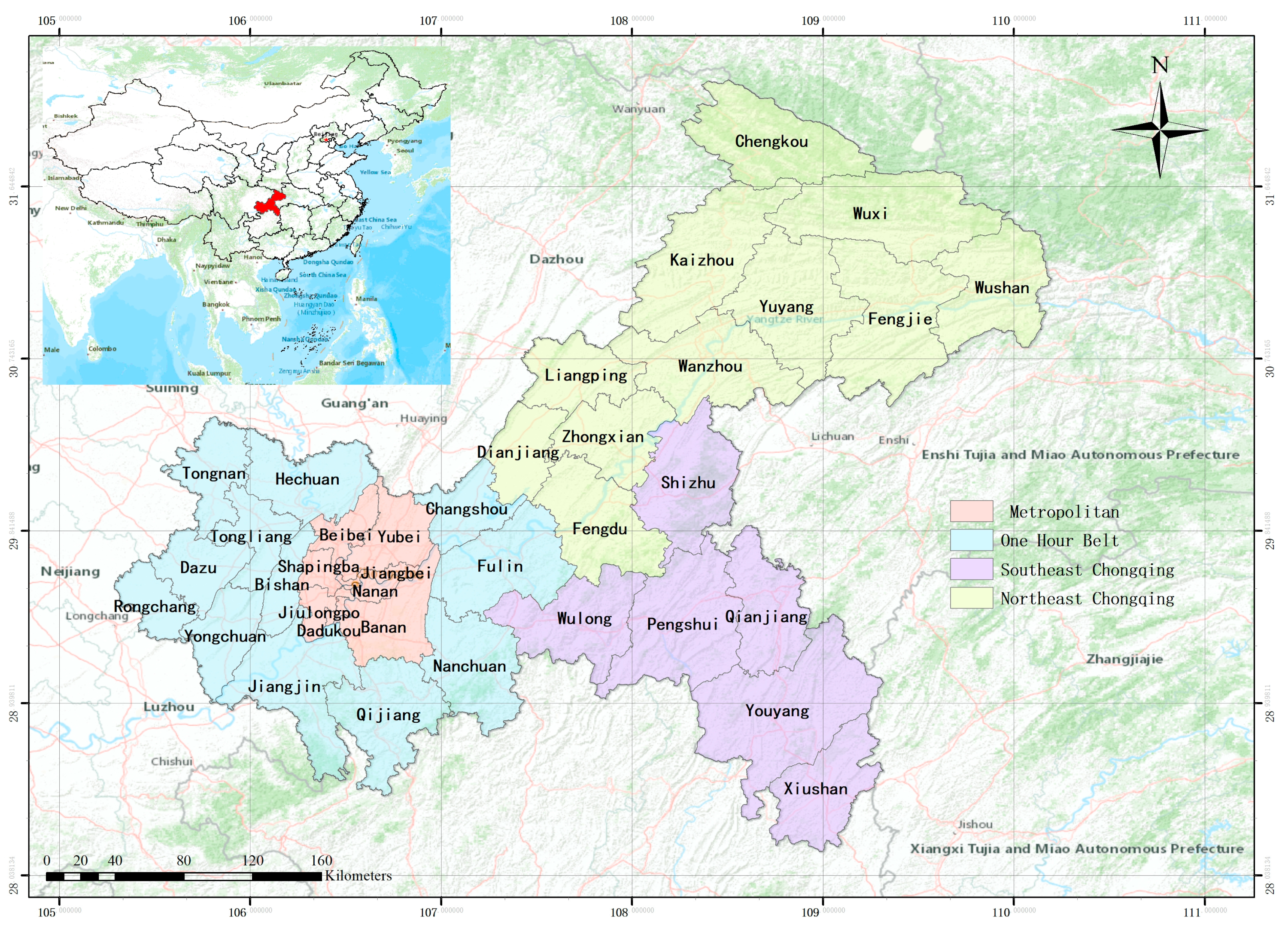
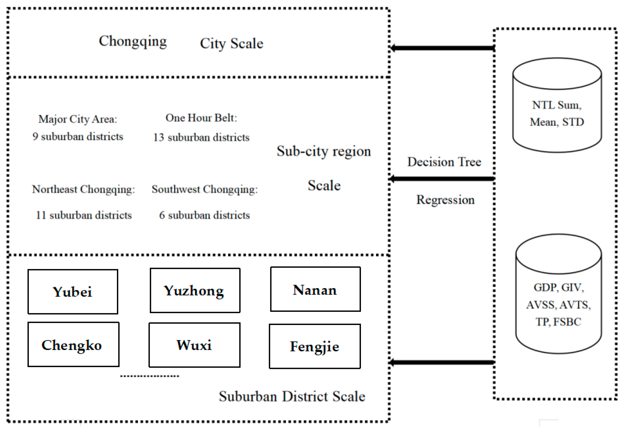
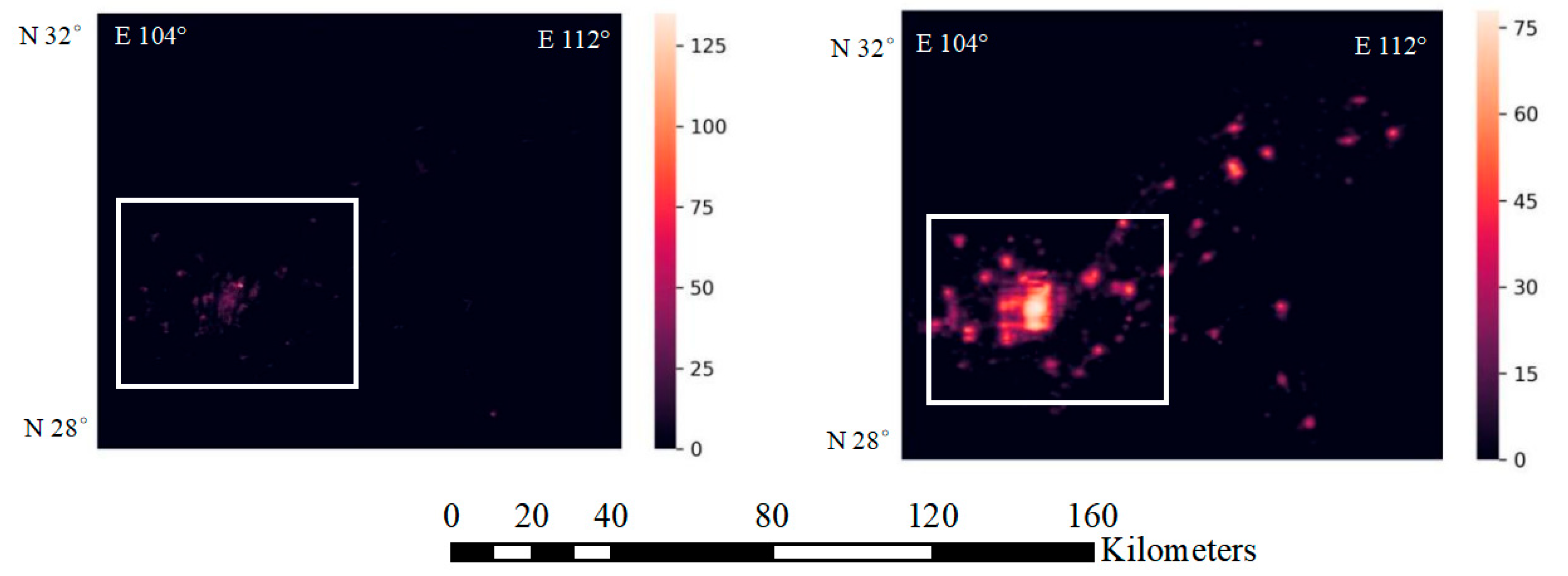
2.1. Study Area
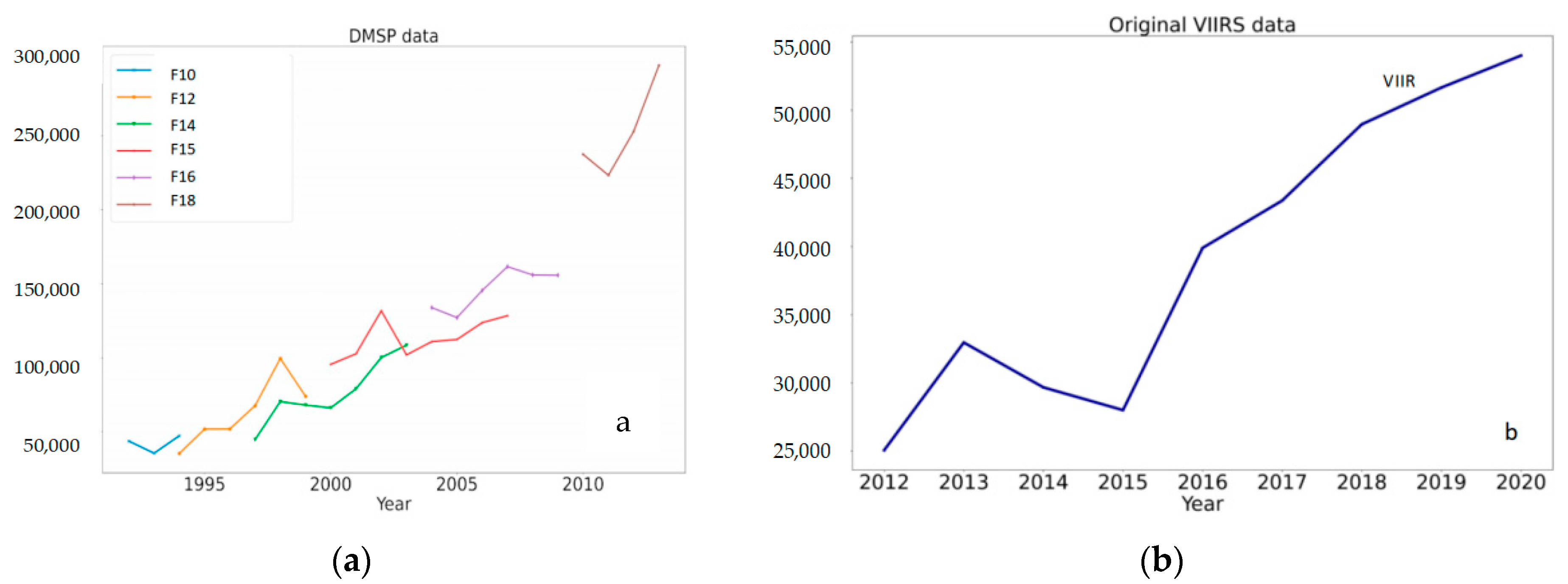
2.2. Used Data
3. Methodology
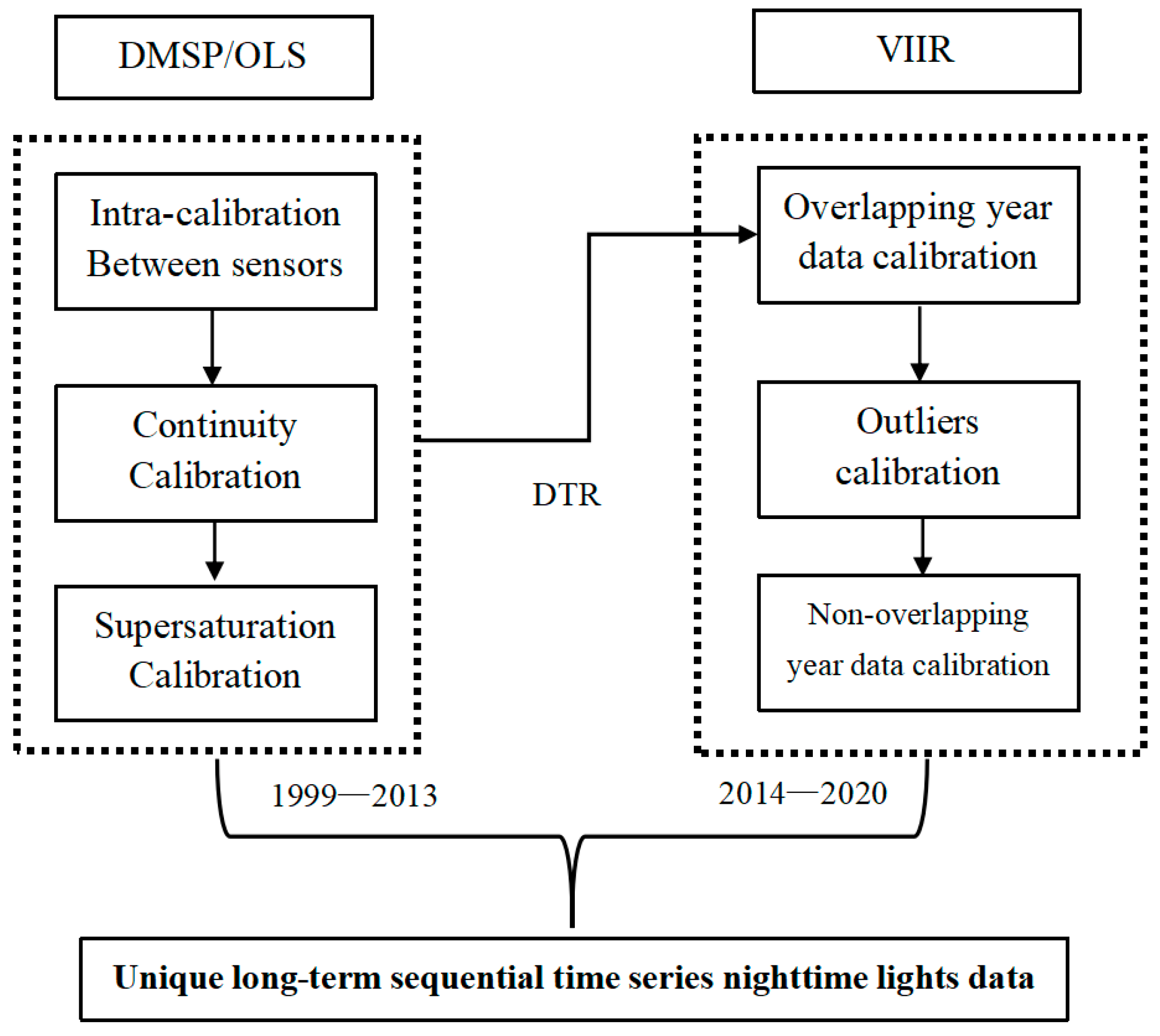
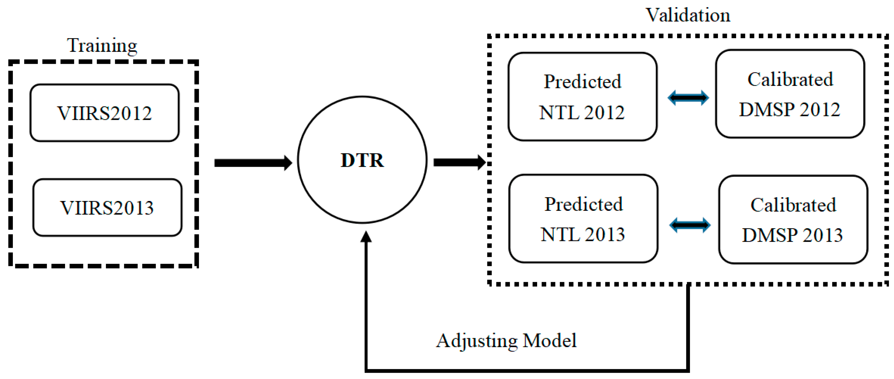
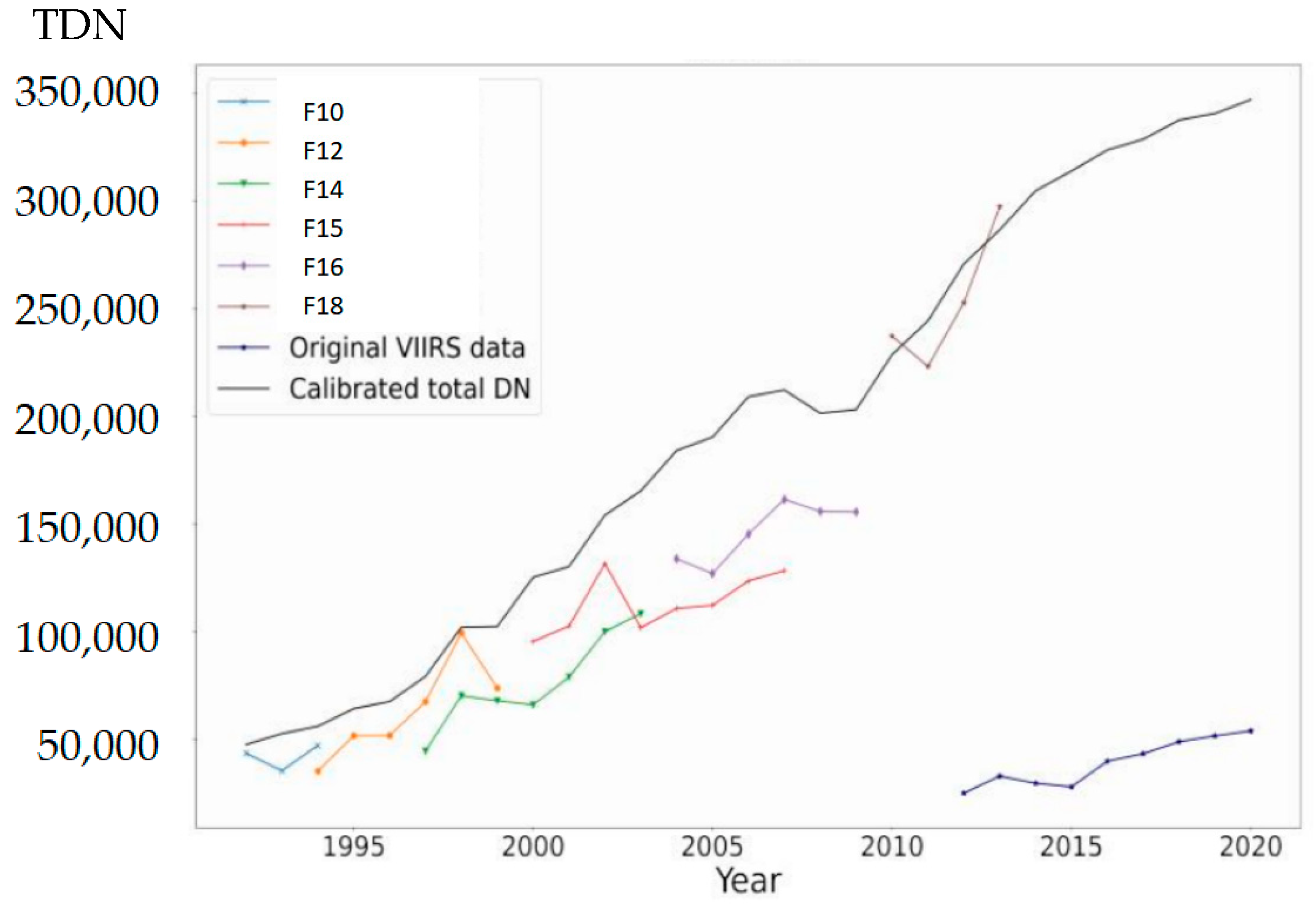
3.1. NTL Data Calibration Process
- (1)
- DMSP/OLS data calibration
- (2)
- VIIRS data calibration
3.2. Spatiotemporal Analysis
4. Results
4.1. NTL Data Calibration Results
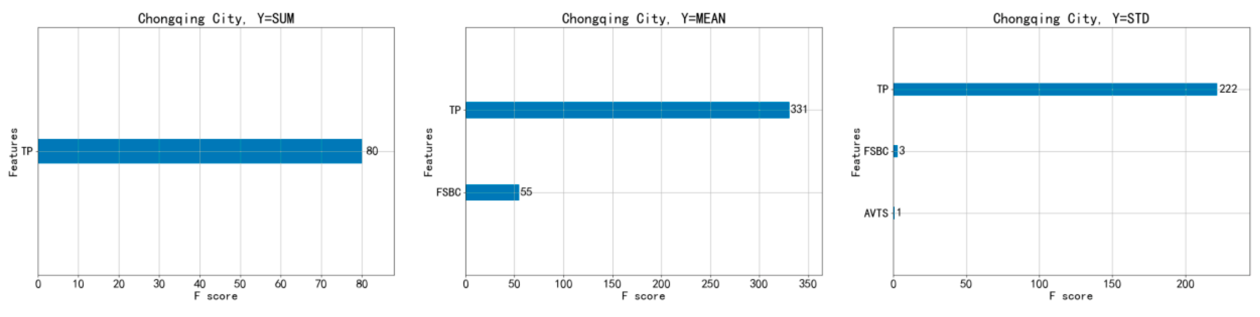
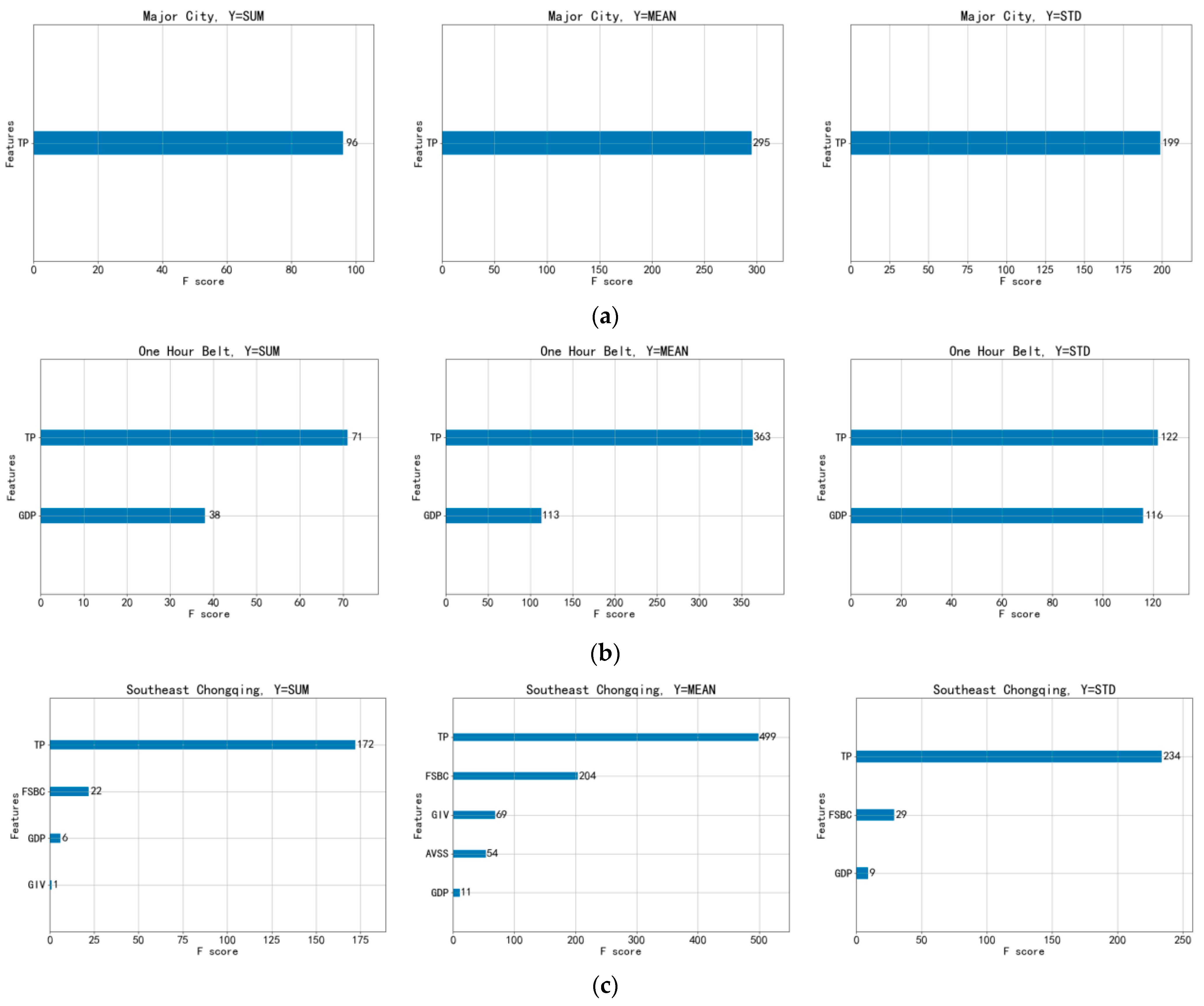
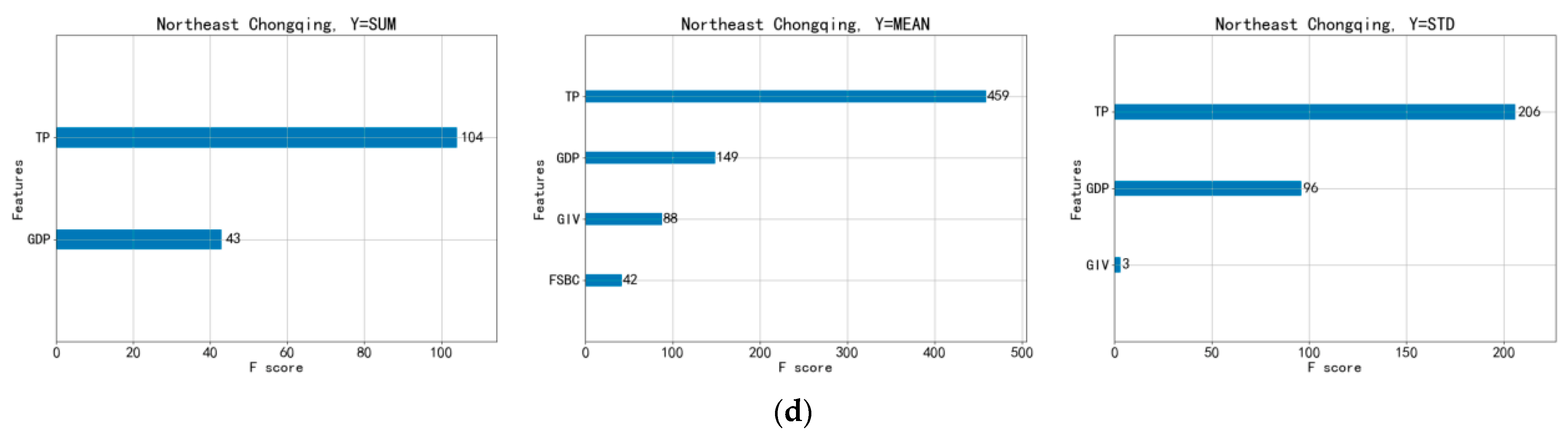
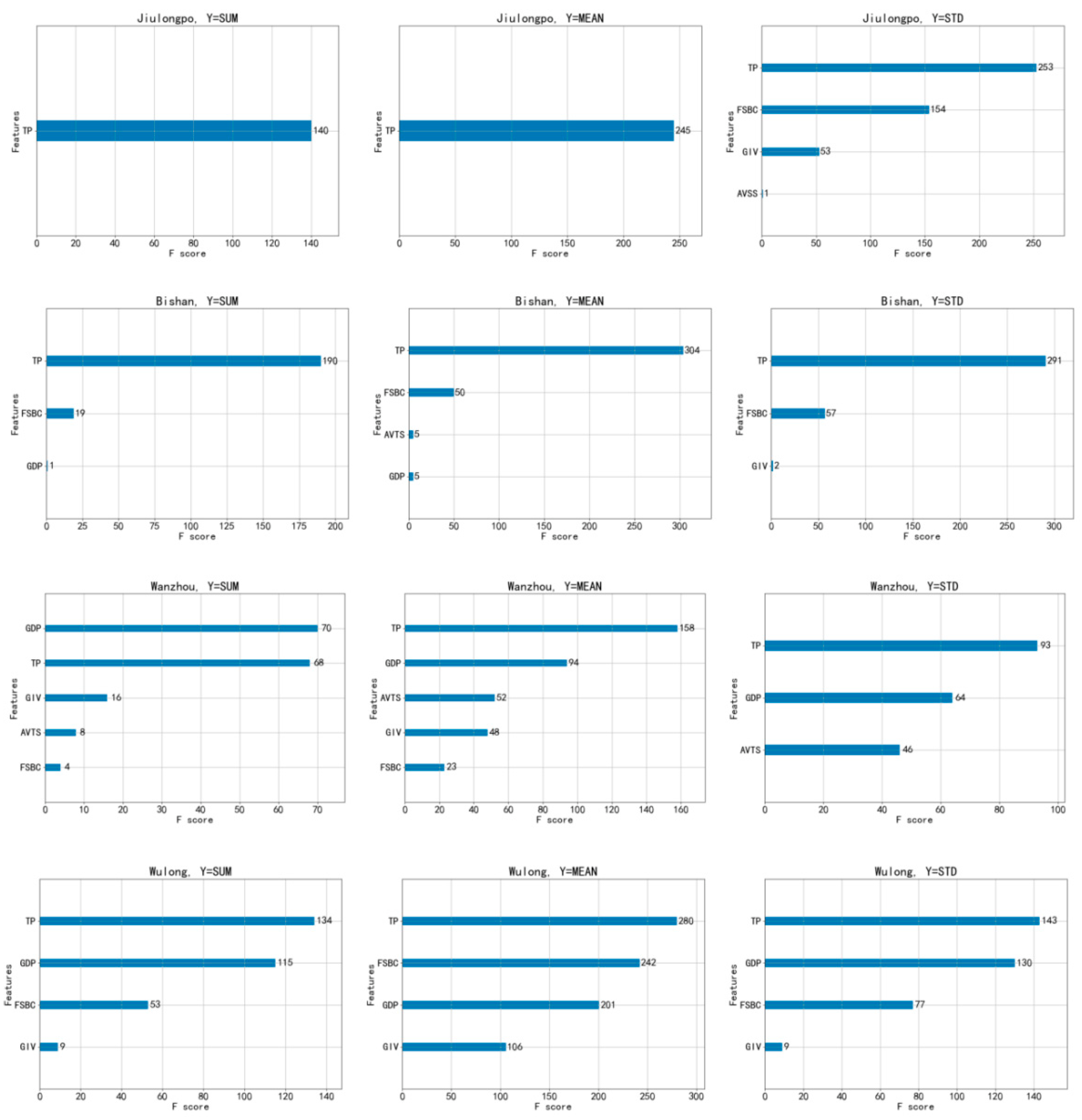
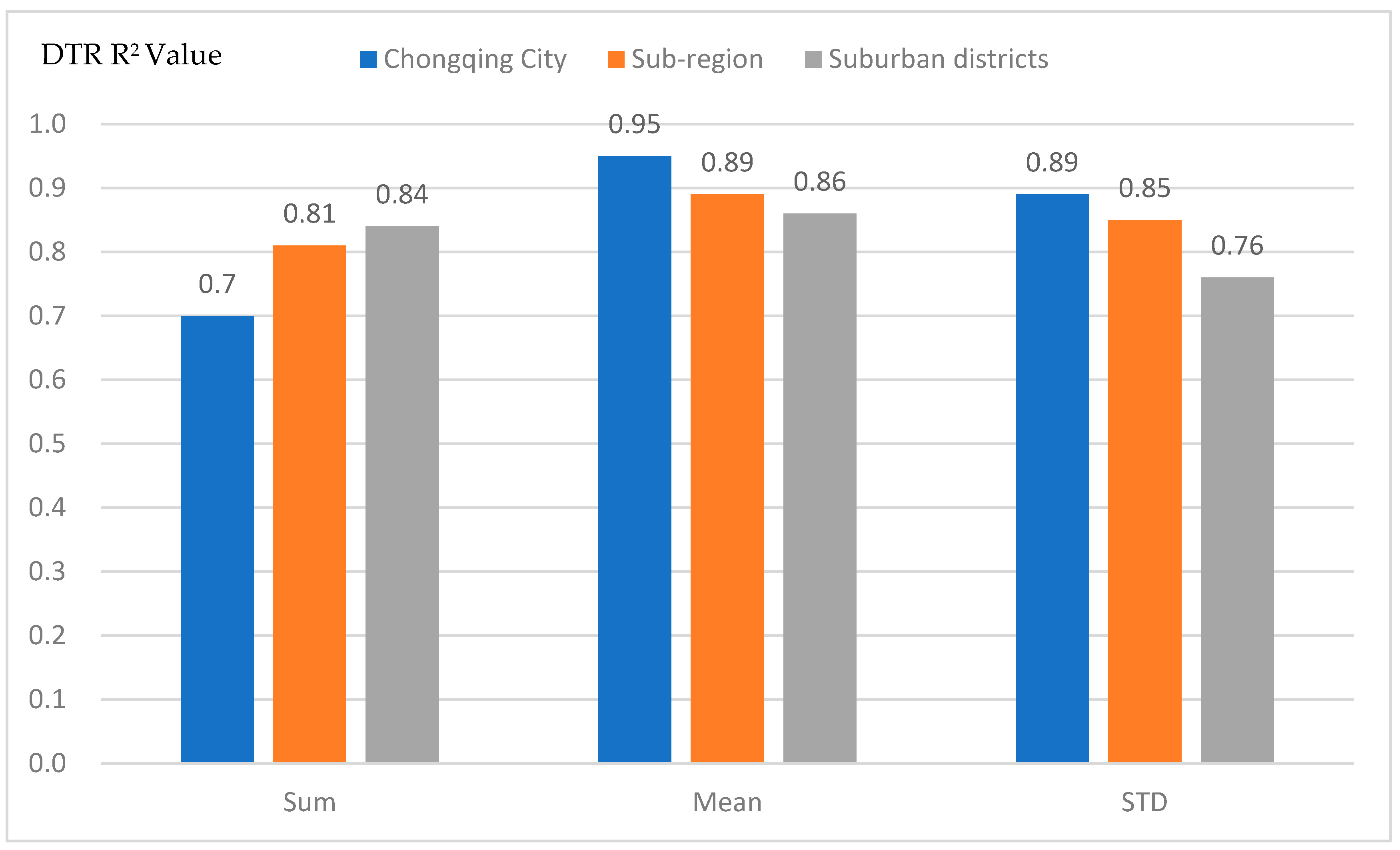
4.2. NTL Decision Tree Regression Results
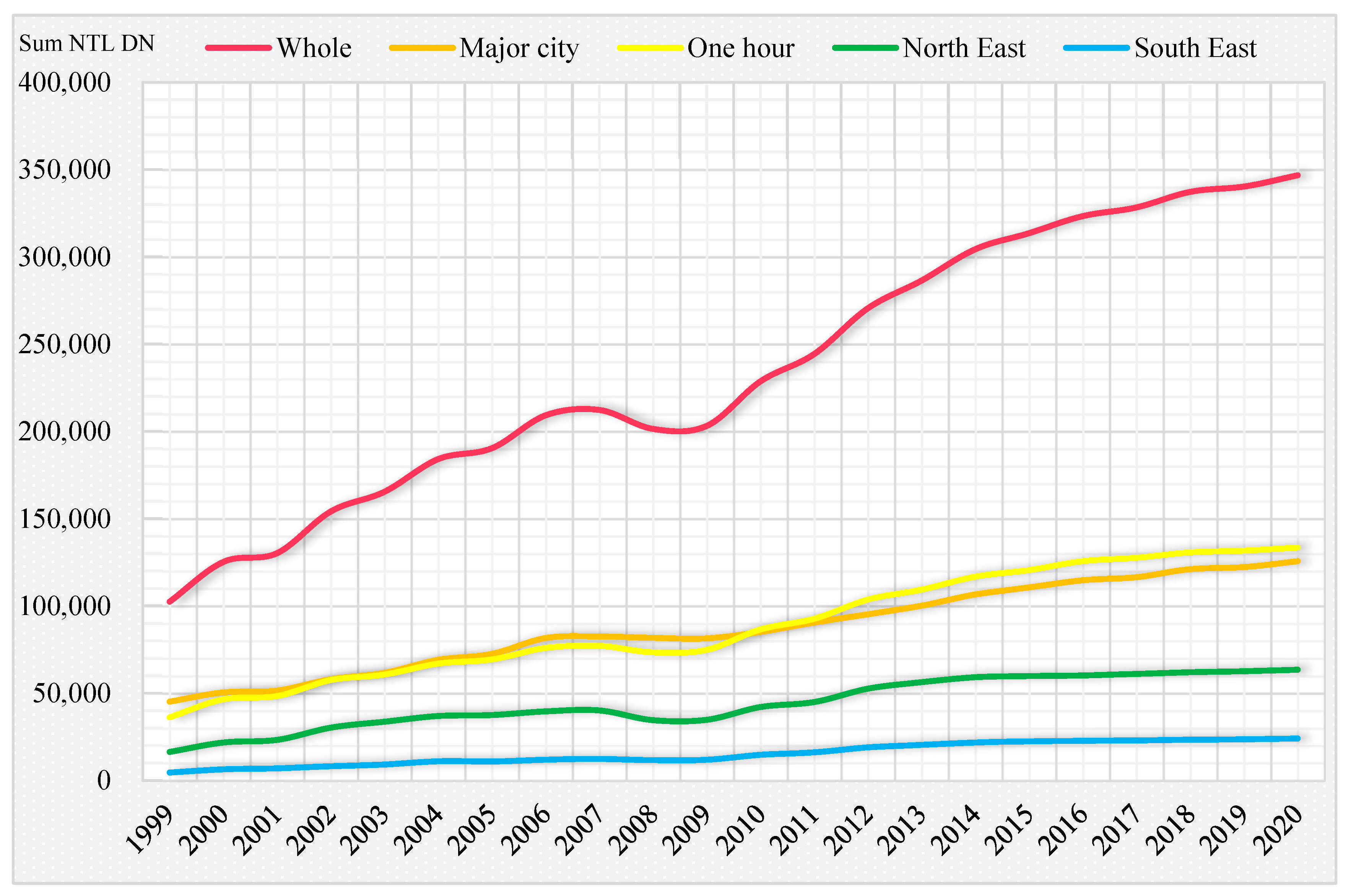
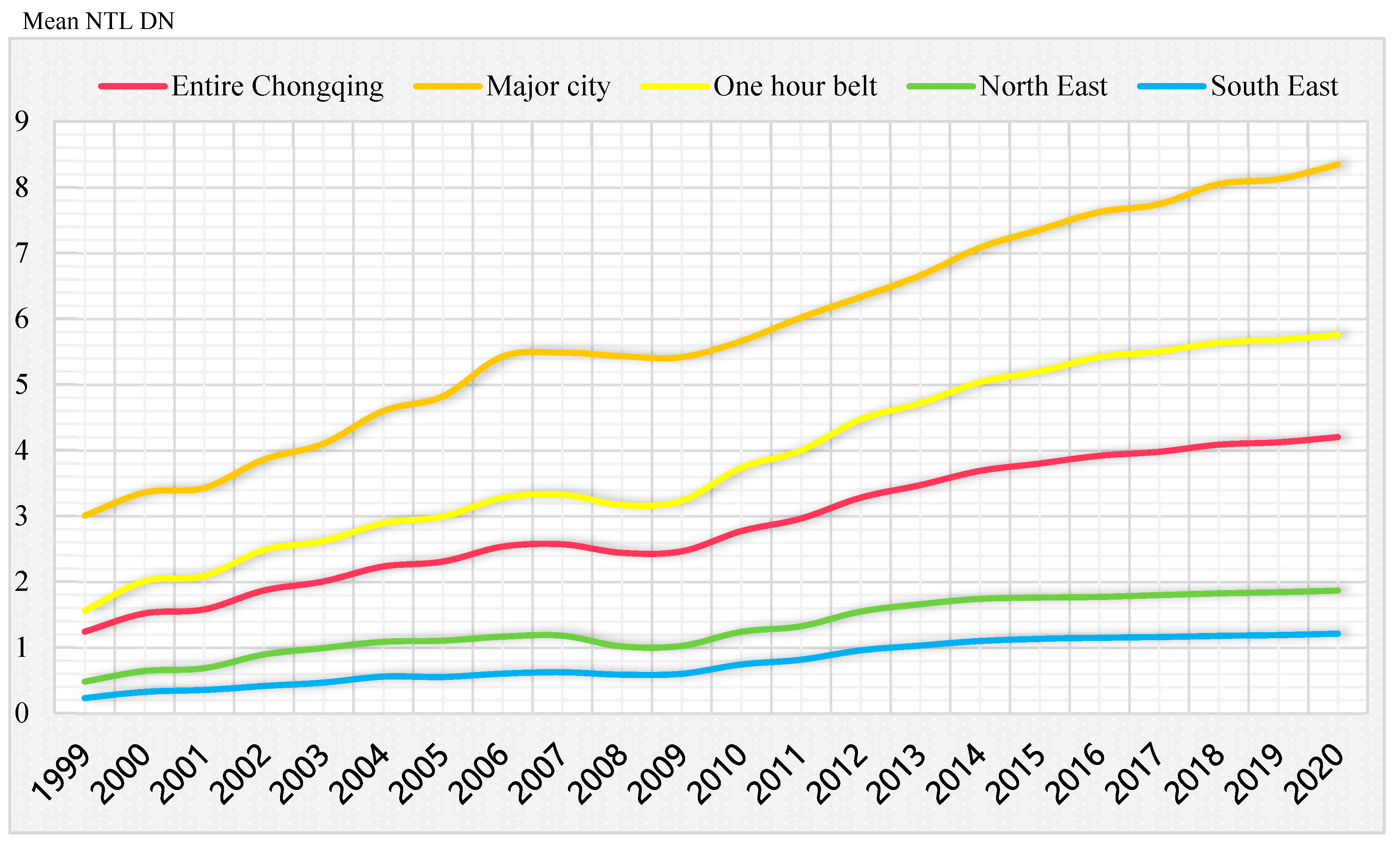
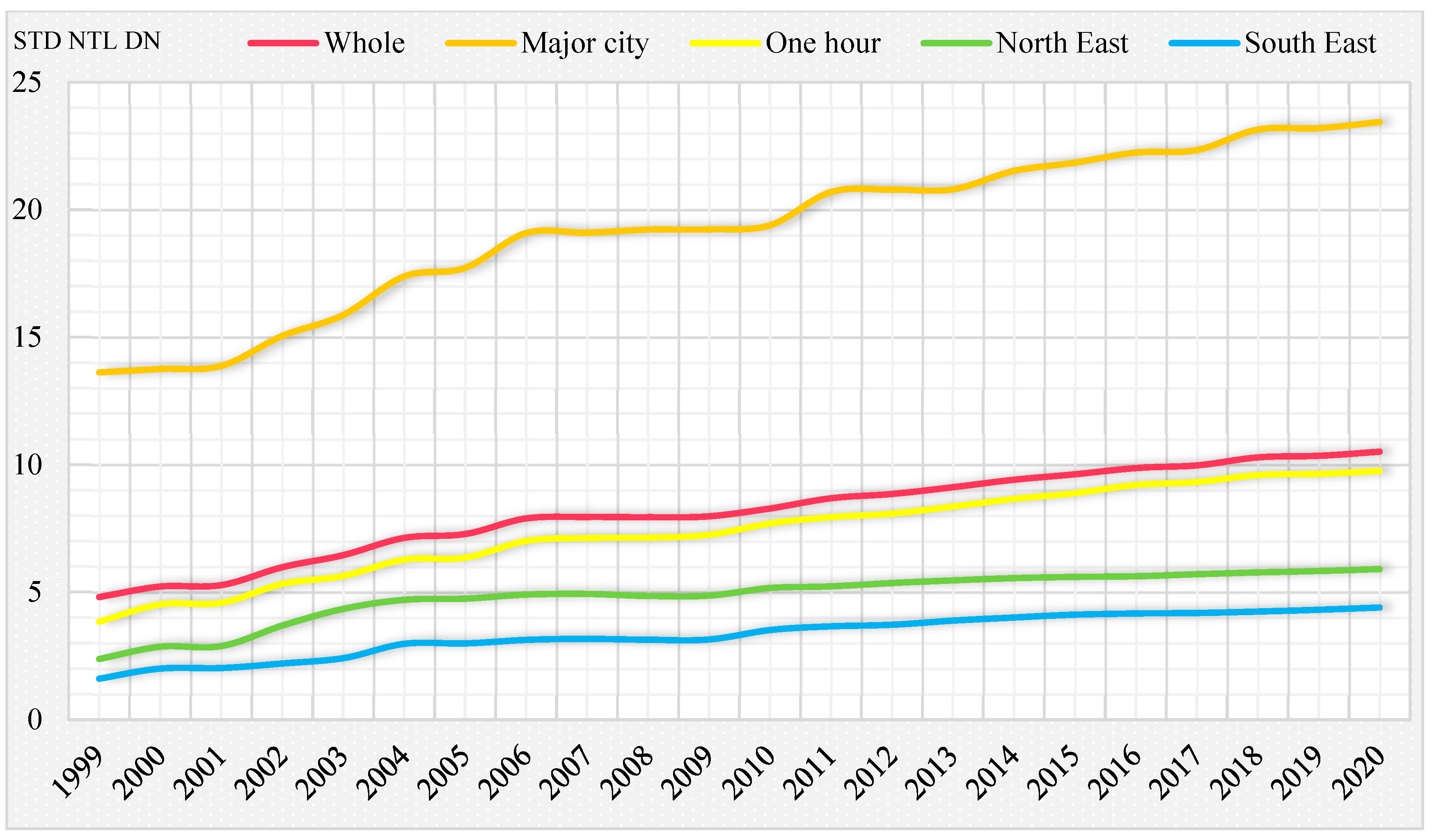
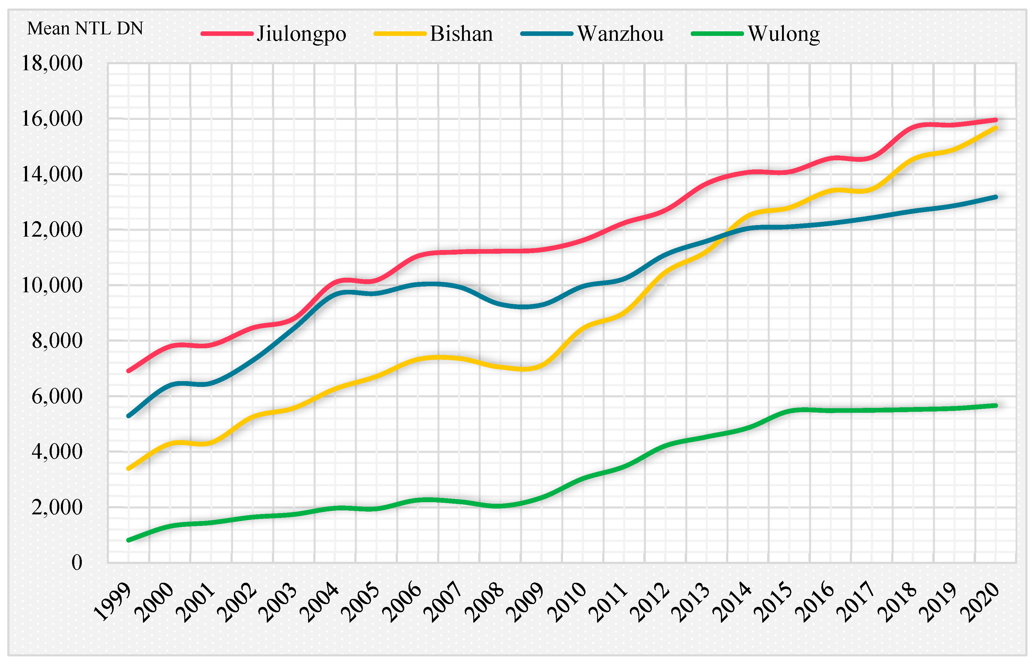
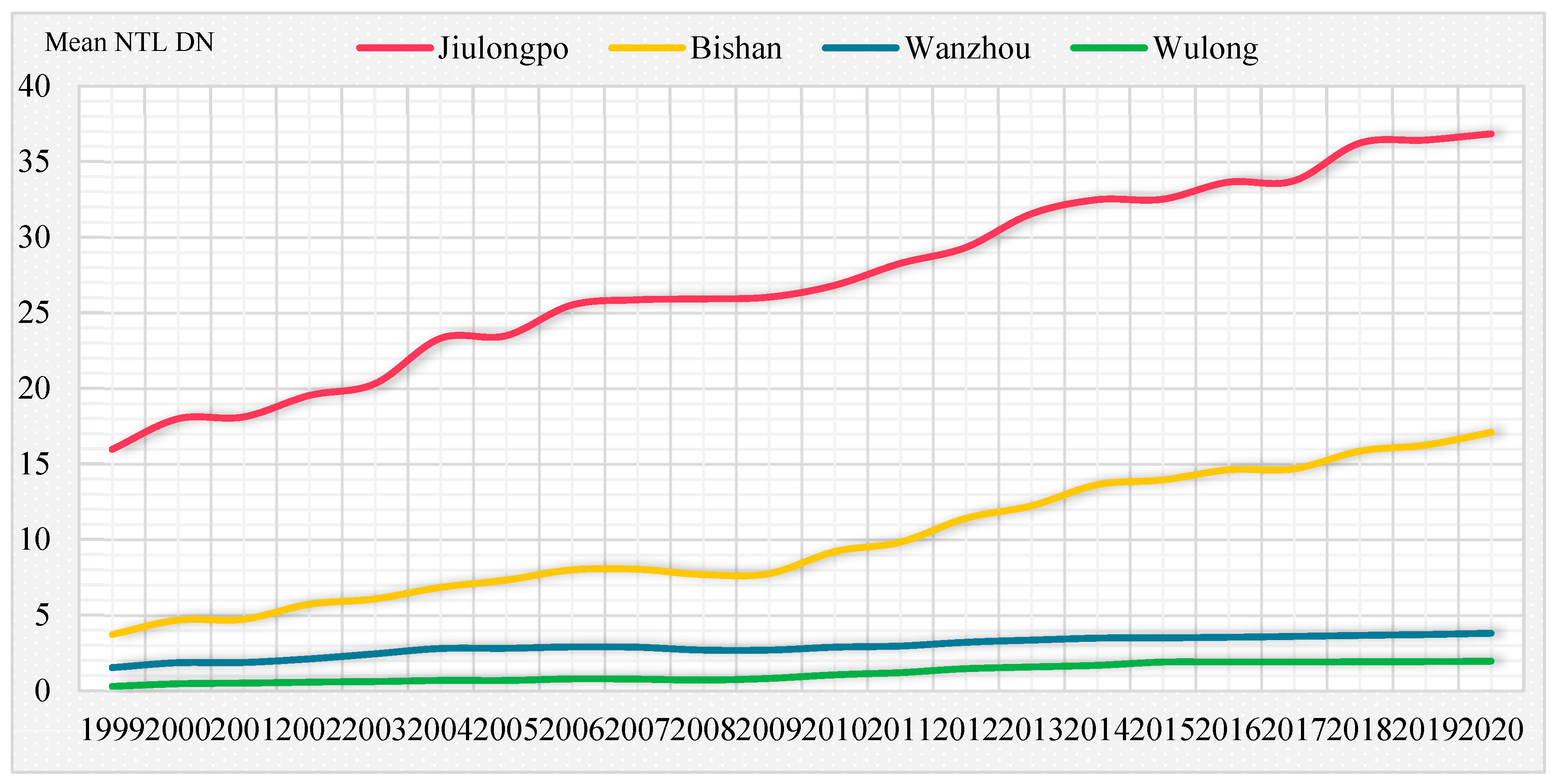
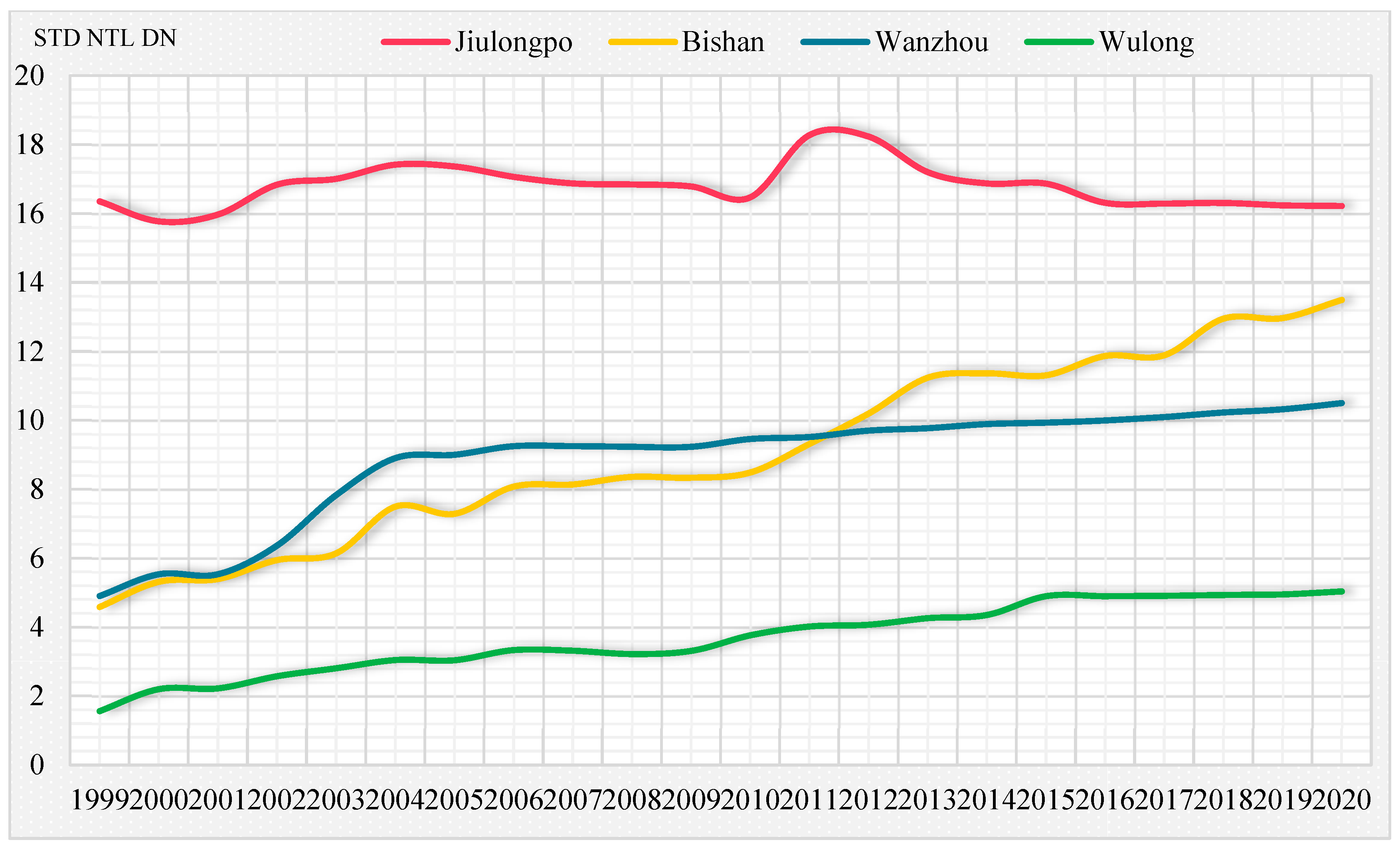
4.3. Multi-Scale Analysis of NTL Data
5. Discussion
6. Conclusions
Supplementary Materials
Author Contributions
Funding
Institutional Review Board Statement
Informed Consent Statement
Data Availability Statement
Acknowledgments
Conflicts of Interest
References
- Min, B.; Gaba, K.M.; Sarr, O.F.; Agalassou, A. Detection of rural electrification in africa using dmsp-ols night lights imagery. Int. J. Remote Sens. 2013, 34, 8118–8141. [Google Scholar] [CrossRef]
- Xu, T.; Coco, G.; Gao, J. Extraction of urban built-up areas from nighttime lights using artificial neural network. Geocarto Int. 2020, 35, 1049–1066. [Google Scholar]
- Zhu, Z.; Zhou, Y.; Seto, K.C.; Stokes, E.C.; Deng, C.; Pickett, S.T.; Taubenböck, H. Understanding an urbanizing planet: Strategic directions for remote sensing. Remote Sens. Environ. 2019, 228, 164–182. [Google Scholar] [CrossRef]
- Elvidge, C.D.; Baugh, K.E.; Kihn, E.A.; Kroehl, H.W.; Davis, E.R.; Davis, C.W. Relation between satellite observed visiblenear infrared emissions, population, economic activity and electric power consumption. Int. J. Remote Sens. 1997, 18, 1373–1379. [Google Scholar] [CrossRef]
- Aubrecht, C.; Elvidge, C.D.; Ziskin, D.; Baugh, K.E.; Tuttle, B.T.; Erwin, E.; Kerle, N. Observing power blackouts from space—A disaster related study. In EGU General Assembly: Geophysical Research Abstracts; European Geosciences Union: Vienna, Austria, 2009; pp. 1–2. [Google Scholar]
- Witmer, F.; Loughlin, O. Detecting the effects of wars in the caucasus regions of russia and georgia using radiometrically normalized dmsp-ols nighttime lights imagery. GISci. Remote Sens. 2022, 48, 478–500. [Google Scholar] [CrossRef]
- Xi, L.; Chen, F.; Chen, X. Satellite-observed nighttime light variation as evidence for global armed conflicts. IEEE J. Sel. Top. Appl. Earth Obs. Remote Sens. 2013, 6, 2302–2315. [Google Scholar]
- Bennie, J.; Davies, T.; Inger, R.; Gaston, K.J. Mapping artificial lightscapes for ecological studies. Methods Ecol. Evol. 2014, 5, 203–214. [Google Scholar] [CrossRef]
- Doll, C.H.; Muller, J.P.; Elvidge, C.D. Night-time imagery as a tool for global mapping of socioeconomic parameters and greenhouse gas emissions. Ambio 2000, 29, 157–162. [Google Scholar]
- Doll, C.N.; Muller, J.P.; Morley, J.G. Mapping regional economic activity from night-time light satellite imagery. Ecol. Econ. 2006, 57, 75–92. [Google Scholar] [CrossRef]
- Vernon, H.J.; Storeygard, A.; Weil, D.N. Measuring Economic Growth from Outer Space. Am. Econ. Rev. 2012, 102, 994–1028. [Google Scholar]
- Xu, P.; Jin, P.; Yang, Y.; Quan, W. Evaluating urbanization and spatial-temporal pattern using the dmsp/ols nighttime light data: A case study in zhejiang province. Math. Probl. Eng. 2016, 2016, 9850890. [Google Scholar] [CrossRef] [Green Version]
- Clark, H.; Pinkovskiy, M.; Sala-i-Martin, X. China’s GDP Growth Maybe Understated; National Bureau of Economic Research: Cambridge, MA, USA, 2017. [Google Scholar]
- Xi, L.; Xu, H.; Chen, X.; Li, C. Potential of npp-viirs nighttime light imagery for modeling the regional economy of china. Remote Sens. 2013, 5, 3057–3081. [Google Scholar]
- Ghosh, T.; Powell, R.L.; Elvidge, C.D.; Baugh, K.E.; Sutton, P.C.; Anderson, S. Shedding light on the global distribution of economic activity. Open Geogr. J. 2010, 3, 147–160. [Google Scholar]
- Liao, L.B.; Weiss, S.; Mills, S.; Hauss, B. Suomi npp viirs day-night band on-orbit performance. J. Geophys. Res. Atmos. 2013, 118, 12705–12718. [Google Scholar] [CrossRef]
- Elvidge, C.D.; Baugh, K.; Zhizhin, M.; Hsu, F.; Ghosh, T. VIIRS night-time lights. Int. J. Remote Sens. 2017, 38, 5860–5879. [Google Scholar] [CrossRef] [Green Version]
- Elvidge, C.D.; Baugh, K.; Zhizhin, M.; Hsu, F.C. Why viirs data are superior to dmsp for mapping nighttime lights. Proc. Asia Pac. Adv. Netw. 2013, 35, 62–69. [Google Scholar] [CrossRef]
- Zhao, M.; Cheng, W.; Zhou, C.; Li, M.; Nan, W.; Liu, Q. Gdp spatialization and economic differences in south china based on npp-viirs nighttime light imagery. Remote Sens. 2017, 9, 673. [Google Scholar] [CrossRef] [Green Version]
- Forbes, D.J. Multi-scale analysis of the relationship between economic statistics and dmsp-ols night light images. Mapp. Sci. Remote Sens. 2013, 50, 483–499. [Google Scholar] [CrossRef]
- Zhao, M.; Zhou, Y.; Li, X.; Zhou, C.; Huang, K. Building a series of consistent night-time light data (1992–2018) in southeast asia by integrating dmsp-ols and npp-viirs. IEEE Trans. Geosci. Remote Sens. 2019, 58, 1843–1856. [Google Scholar] [CrossRef]
- Bian, J.; Li, A.; Lei, G.; Zhang, Z.; Liang, L. Intercalibration of nighttime light data between dmsp/ols and npp/viirs in the economic corridors of belt and road initiative. In Proceedings of the IGARSS 2019—2019 IEEE International Geoscience and Remote Sensing Symposium, Yokohama, Japan, 28 July–2 August 2019. [Google Scholar]
- Li, X.; Li, D.; Xu, H.; Wu, C. Intercalibration between DMSP/OLS and VIIRS night-time light images to evaluate city light dynamics of Syria’s major human settlement during Syrian Civil War. Int. J. Remote Sens. 2017, 38, 5934–5951. [Google Scholar] [CrossRef]
- Yong, Z.; Li, K.; Xiong, J.; Cheng, W.; Wang, Z.; Sun, H.; Ye, C. Integrating DMSP-OLS and NPP-VIIRS Nighttime Light Data to Evaluate Poverty in Southeastern China. Remote Sens. 2022, 14, 600. [Google Scholar] [CrossRef]
- Levin, N.; Kyba, C.C.M.; Zhang, Q.; Sánchez de Miguel, A.; Román, M.O.; Li, X.; Portnov, B.A.; Molthan, A.L.; Jechow, A.; Miller, S.D.; et al. Remote sensing of night lights: A review and an outlook for the future. Remote Sens. Environ. 2020, 237, 111443. [Google Scholar] [CrossRef]
- Ma, J.; Guo, J.; Ahmad, S.; Li, Z.; Hong, J. Constructing a new inter-calibration method for DMSP-OLS and NPP-VIIRS nighttime light. Remote Sens. 2020, 12, 937. [Google Scholar] [CrossRef] [Green Version]
- Ge, X. Research on GDP Forecast Model Based on DMSP/OLS Night Light Image. Surv. Mapp. Spat. Geogr. Inf. 2019, 42, 181–183+190. [Google Scholar]
- Han, G.; Zhou, T.; Sun, Y.; Zhu, S. The relationship between night-time light and socioeconomic factors in China and India. PLoS ONE 2022, 17, e0262503. [Google Scholar] [CrossRef]
- Letu, H.; Hara, M.; Tana, G.; Nishio, F. A saturated light correction method for dmsp/ols nighttime satellite imagery. IEEE Trans. Geosci. Remote Sens. 2011, 50, 389–396. [Google Scholar] [CrossRef]
- Jiang, L.; Liu, Y.; Wu, S.; Yang, C. Study on Urban Spatial Pattern Based on DMSP/OLS and NPP/VIIRS in Democratic People’s Republic of Korea. Remote Sens. 2021, 13, 4879. [Google Scholar] [CrossRef]
- Wu, K.; Wang, X. Aligning Pixel Values of DMSP and VIIRS Nighttime Light Images to Evaluate Urban Dynamics. Remote Sens. 2019, 11, 1463–1478. [Google Scholar] [CrossRef] [Green Version]
- Hu, Y.; Zhang, Y. Global nighttime light change from 1992 to 2017: Brighter and more uniform. Sustainability 2020, 12, 4905. [Google Scholar] [CrossRef]
- Jiang, L.; Yang, C.; Liu, Y. Spatial and temporal changes of Laos’ economic and social development from 1992 to 2020 based on night light data. Resour. Sci. 2021, 43, 2381–2392. [Google Scholar]
- Xu, P.; Jin, P.; Cheng, Q.; Stanisławski, R. Monitoring Regional Urban Dynamics Using DMSP/OLS Nighttime Light Data in Zhejiang Province. Math. Probl. Eng. 2020, 2020, 9652808. [Google Scholar] [CrossRef]
- Shao, Z.; Tang, Y.; Huang, X.; Li, D. Monitoring Work Resumption of Wuhan in the COVID-19 Epidemic Using Daily Nighttime Light. Photogramm. Eng. Remote Sens. 2021, 87, 195–204. [Google Scholar] [CrossRef]
- Anoop, V.; Bipin, P.R. Retraction Note: Medical Image Enhancement by a Bilateral Filter Using Optimization Technique. J. Med. Syst. 2022, 46, 240. [Google Scholar] [CrossRef] [PubMed]
- Wei, Y.; Zhu, Y.; Cao, J. Research on multilevel median filtering algorithm for seismic data. J. Hebei Univ. Geosci. 2022, 45, 68–74. [Google Scholar]
- Li, X.; Lu, G. Correction and fitting of night light images of DMSP/OLS and VIIRS/DNB. Bull. Surv. Mapp. 2019, 7, 138–146. [Google Scholar]
- Wu, J.; He, S.; Peng, J.; Li, W.; Zhong, X. Intercalibration of DMSP-OLS night-time light data by the invariant region method. Int. J. Remote Sens. 2013, 34, 7356–7368. [Google Scholar] [CrossRef]
- Cao, Z.; Wu, Z.; Kuang, Y.Q.; Huang, N. Correction of dmsp/ols night-time light images and its application in china. J. Geo-Inf. Sci. 2015, 17, 1092–1102. [Google Scholar]
- Zhuo, L.; Zhang, X.; Zheng, J.; Tao, H.; Guo, Y. An evi-based method to reduce saturation of dmsp/ols nighttime light data. Acta Geogr. Sin. 2015, 70, 1339–1350. [Google Scholar]
- Wang, Q.; Yuan, T.; Zheng, X.Q. GDP gross analysis at province-level in China based on night-time light satellite imagery. Urban Dev. Stud. 2013, 20, 44–48. [Google Scholar]
- Safavian, S.; Landgrebe, D. A survey of decision tree classifier methodology. IEEE Trans. Syst. Man Cybern. 1991, 21, 660–674. [Google Scholar] [CrossRef] [Green Version]
- Tomasi, C.; Manduchi, R. Bilateral filtering for gray and color images. In Proceedings of the Sixth International Conference on Computer Vision (IEEE Cat. No. 98CH36271), Bombay, India, 7 January 1998; pp. 839–846. [Google Scholar]
- Walker, E. Applied Regression Analysis and Other Multivariable Methods. Technometrics 1989, 31, 117–118. [Google Scholar] [CrossRef]
- Xu, H.; Yang, H.; Li, X.; Jin, H.; Li, D. Multi-scale measurement of regional inequality in Mainland China during 2005–2010 using DMSP/OLS night light imagery and population density grid data. Sustainability 2015, 7, 13469–13499. [Google Scholar] [CrossRef] [Green Version]
- Small, C.; Elvidge, C.D. Night on Earth: Mapping decadal changes of anthropogenic night light in Asia. Int. J. Appl. Earth Obs. Geoinf. 2013, 22, 40–52. [Google Scholar] [CrossRef]
- Hopkins, G.R.; Gaston, K.J.; Visser, M.E.; Elgar, M.A.; Jones, T.M. Artificial light at night as a driver of evolution across urban–rural landscapes. Front. Ecol. Environ. 2018, 16, 472–479. [Google Scholar] [CrossRef] [Green Version]
- Chen, Z.; Yu, B.; Yang, C.; Zhou, Y.; Yao, S.; Qian, X.; Wang, C.; Wu, B.; Wu, J. An extended time series (2000–2018) of global NPP-VIIRS-like nighttime light data from a cross-sensor calibration. Earth Syst. Sci. Data 2021, 13, 889–906. [Google Scholar] [CrossRef]
- Cao, C.; Zhang, B.; Xia, F.; Bai, Y. Exploring VIIRS Night Light Long-Term Time Series with CNN/SI for Urban Change Detection and Aerosol Monitoring. Remote Sens. 2022, 14, 3126. [Google Scholar] [CrossRef]
- Cavazzani, S.; Ortolani, S.; Bertolo, A.; Binotto, R.; Fiorentin, P.; Carraro, G.; Zitelli, V. Satellite measurements of artificial light at night: Aerosol effects. Mon. Not. R. Astron. Soc. 2020, 499, 5075–5089. [Google Scholar] [CrossRef]


| Sensor | Year | a | b | c | R2 |
|---|---|---|---|---|---|
| F10 | 1992 | −0.0031 | 1.2854 | 0.5164 | 0.7972 |
| 1993 | −0.0014 | 1.1634 | 1.3032 | 0.8045 | |
| 1994 | 0.0022 | 0.9531 | 0.8577 | 0.8198 | |
| F12 | 1994 | 0.0021 | 0.9781 | 1.9929 | 0.7982 |
| 1995 | 0.0065 | 0.6991 | 3.9826 | 0.8016 | |
| 1996 | 0.0093 | 0.5627 | 4.2085 | 0.8156 | |
| 1997 | 0.0104 | 0.4209 | 6.9318 | 0.8104 | |
| 1998 | 0.0118 | 0.4764 | 6.2895 | 0.8139 | |
| 1999 | 0.0082 | 0.6057 | 3.9276 | 0.8348 | |
| F14 | 1997 | 0.0054 | 0.7886 | 2.5985 | 0.8268 |
| 1998 | 0.0061 | 0.7543 | 2.9812 | 0.7986 | |
| 1999 | 0.0009 | 1.0246 | 2.9390 | 0.8420 | |
| 2000 | 0.0054 | 0.7861 | 9.0337 | 0.8541 | |
| 2001 | 0.0003 | 1.2143 | 1.1397 | 0.8489 | |
| 2002 | 0.0000 | 1.2377 | 0.7930 | 0.8103 | |
| 2003 | −0.0032 | 1.4156 | 0.9545 | 0.8802 | |
| F15 | 2000 | 0.0075 | 0.6452 | 3.7070 | 0.8125 |
| 2001 | 0.0098 | 0.5019 | 1.4560 | 0.8520 | |
| 2002 | 0.0000 | 0.9901 | 2.4539 | 0.8379 | |
| 2003 | −0.0039 | 1.3917 | 1.8164 | 0.8357 | |
| 2004 | −0.0084 | 1.8061 | 0.9048 | 0.8298 | |
| 2005 | −0.0051 | 1.5328 | 0.9462 | 0.8298 | |
| 2006 | −0.0042 | 1.6072 | 1.0359 | 0.8039 | |
| 2007 | −0.0089 | 1.8307 | 0.6289 | 0.7961 | |
| F16 | 2004 | −0.0014 | 1.1668 | 1.0703 | 0.8679 |
| 2005 | −0.0028 | 1.4042 | 0.1650 | 0.9102 | |
| 2006 | −0.0051 | 1.5113 | 0.0195 | 0.9348 | |
| 2007 | −0.0000 | 0.0000 | 0.0000 | 0.0000 | |
| 2008 | 0.0056 | 0.6757 | 1.8309 | 0.9242 | |
| 2009 | 0.0071 | 0.5859 | 2.9597 | 0.9251 | |
| F18 | 2010 | 0.0085 | 0.4396 | 306207 | 0.8964 |
| 2011 | 0.0069 | 0.4996 | 3.9897 | 0.7945 | |
| 2012 | 0.0085 | 0.3987 | 4.0598 | 0.8223 | |
| 2013 | 0.0074 | 0.4833 | 2.8755 | 0.8031 |
| NTL Sum | 1st Order | 2nd Order | 3rd Order | Other | Frequency | Average F Score |
|---|---|---|---|---|---|---|
| TP | 30 | 7 | 1 | 0 | 38 | 145 |
| GDP | 8 | 16 | 6 | 2 | 32 | 68 |
| GIV | 0 | 1 | 8 | 12 | 21 | 24 |
| AVSS | 0 | 0 | 1 | 3 | 4 | 17 |
| AVTS | 0 | 0 | 1 | 3 | 4 | 10 |
| FSCB | 0 | 10 | 12 | 5 | 27 | 40 |
| Total | 38 | 34 | 29 | 25 | 126 | |
| NTL Mean | 1st Order | 2nd Order | 3rd Order | Other | Frequency | Average Score |
| TP | 34 | 3 | 1 | 0 | 38 | 282 |
| GDP | 4 | 14 | 9 | 6 | 33 | 104 |
| GIV | 0 | 3 | 5 | 17 | 25 | 64 |
| AVSS | 0 | 0 | 2 | 9 | 11 | 18 |
| AVTS | 0 | 0 | 3 | 5 | 8 | 22 |
| FSCB | 0 | 16 | 13 | 3 | 32 | 92 |
| Total | 38 | 36 | 33 | 40 | 147 | |
| NTL STD | 1st Order | 2nd Order | 3rd Order | Other | Frequency | Average Score |
| TP | 27 | 3 | 0 | 8 | 38 | 164 |
| GDP | 11 | 16 | 3 | 0 | 30 | 96 |
| GIV | 0 | 1 | 12 | 12 | 25 | 23 |
| AVSS | 0 | 2 | 2 | 5 | 9 | 37 |
| AVTS | 0 | 0 | 2 | 1 | 3 | 21 |
| FSCB | 0 | 7 | 11 | 7 | 25 | 43 |
| Total | 38 | 29 | 30 | 33 | 130 |
Disclaimer/Publisher’s Note: The statements, opinions and data contained in all publications are solely those of the individual author(s) and contributor(s) and not of MDPI and/or the editor(s). MDPI and/or the editor(s) disclaim responsibility for any injury to people or property resulting from any ideas, methods, instructions or products referred to in the content. |
© 2023 by the authors. Licensee MDPI, Basel, Switzerland. This article is an open access article distributed under the terms and conditions of the Creative Commons Attribution (CC BY) license (https://creativecommons.org/licenses/by/4.0/).
Share and Cite
Xu, T.; Zong, Y.; Su, H.; Tian, A.; Gao, J.; Wang, Y.; Su, R. Prediction of Multi-Scale Socioeconomic Parameters from Long-Term Nighttime Lights Satellite Data Using Decision Tree Regression: A Case Study of Chongqing, China. Land 2023, 12, 249. https://doi.org/10.3390/land12010249
Xu T, Zong Y, Su H, Tian A, Gao J, Wang Y, Su R. Prediction of Multi-Scale Socioeconomic Parameters from Long-Term Nighttime Lights Satellite Data Using Decision Tree Regression: A Case Study of Chongqing, China. Land. 2023; 12(1):249. https://doi.org/10.3390/land12010249
Chicago/Turabian StyleXu, Tingting, Yunting Zong, Heng Su, Aohua Tian, Jay Gao, Yurui Wang, and Ruiqi Su. 2023. "Prediction of Multi-Scale Socioeconomic Parameters from Long-Term Nighttime Lights Satellite Data Using Decision Tree Regression: A Case Study of Chongqing, China" Land 12, no. 1: 249. https://doi.org/10.3390/land12010249