Article

Reduction in Water Erosion and Soil Loss on Steep Land Managed by Controlled Traffic Farming

1
Institute of Agricultural Engineering, Transport and Bioenergetics, Faculty of Engineering, Slovak University of Agriculture in Nitra, Tr. A. Hlinku 2, 949 76 Nitra, Slovakia
2
Department of Agricultural Machines, Faculty of Engineering, Czech University of Life Sciences, Kamýcká 129, Suchdol, 165 21 Prague, Czech Republic
3
Institute of Landscape Engineering, Faculty of Horticulture and Landscape Engineering, Slovak University of Agriculture in Nitra, Tr. A. Hlinku 2, 949 76 Nitra, Slovakia
4
Department of Agriculture and Environment, Harper Adams University, Edgmond, Newport TF10 8NB, UK
*
Author to whom correspondence should be addressed.
Land 2023, 12(1), 239; https://doi.org/10.3390/land12010239
Submission received: 21 October 2022 / Revised: 31 December 2022 / Accepted: 9 January 2023 / Published: 12 January 2023

Abstract

:
Controlled traffic farming (CTF) is used to confine soil compaction to the least possible area of the field, thereby achieving economic and environmental benefits. In the context of climate change, soil erosion is one of the most discussed topics, and there is a research gap in understanding the effects of CTF on soil erosion in Central Europe. The aim of this work was to show the potential of CTF to reduce water erosion, in terms of water runoff and soil loss on steep land. A 16 ha experimental field with a CTF technology implemented since 2009 at the Slovak University of Agriculture was used in this research. Three traffic intensity locations were selected and watered using a rainfall simulator. The results showed that the soil which had not been wheeled for 12 years had the lowest water runoff: its intensity after 20 min of simulated rain was 10 times lower compared to the multiple traffic treatment. The soil loss, expressed as the total soil sediments collected after 35 min, in the no traffic area was lower by 70%, compared to the soil with one-pass treatment and only 25% of the loss in the multiple traffic areas. These results show that CTF can significantly reduce soil loss through water runoff on steep land.

1. Introduction

Soil compaction caused by machinery wheels affects the crop production role of soil, e.g., soil water and nutrient availability, natural biological activity, and vulnerability to soil erosion [1,2]. In traditional farming, almost all the field area is subjected to the traffic of agricultural machinery [3,4]. Controlled traffic farming (CTF) is a technology which minimises the compacted area of the field by using permanent tramlines to conduct all crop operations [5]. In random (conventional) traffic farming (RTF), machinery can wheel up to 88% of the soil yearly if ploughing is carried out. This area decreases to 73% and 56% of the field if a minimum or no tillage (direct drilling) system is implemented [3]. On the contrary, CTF leaves 80–90% of fields permanently without soil compaction. In order to achieve this, the implement and machinery widths must be matched. The main advantage of CTF is confining the soil compaction due to machinery movement to the least possible area. This area is constituted by permanent tramlines that can be cultivated (intermediate permanent tramlines) or used only for traffic without cultivation. In CTF, the traffic area of the field goes down to approximately 15%. Thus, the soil with no traffic benefits from better soil structure, lower fuel consumption, and higher crop yield. Published results report crop yield increases up to 25%, depending on the crop and location [4], together with yield stability increases, confirmed in dry growing seasons [6,7]. Other benefits of CTF are decreases of energy consumption, due to reduction of tilled areas; lower soil resistance, resulting from avoiding compaction; lower rolling resistance and wheel slip on permanent tramlines; and enhanced fertiliser use efficiency [8,9,10]. These have been summarised by Tullberg et al. [11] and Antille et al. [1].
CTF can be combined with soil conservation methods used for crop establishment [12]. Even if some farmers fear the initial decrease in crop yield when converting to a non-plough-based tillage, this decrease is compensated by lower production cost and yield increases after the initial 5–7 years [13,14,15]. The benefits from soil conservation methods increase when they are combined with CTF [14], as avoiding traffic increases the benefits from zero tillage.
Avoiding field traffic has positive effects on the environment, especially in terms of greenhouse gas (GHG) emissions reduction [16,17,18], which is critical in relation to climate change. Moreover, soil erosion and loss are a critical issue in today’s farming [15,19].
Gasso 2013 [16] summarised results from Australia and China showing that CTF causes, in general, significant reductions in water runoff (by 28–42%) [20,21,22]. Additionally, the direction of permanent traffic lines has been discussed in the literature with contradictory results. In 2004, Titmarch et al. [23] showed that water runoff and soil erosion levels were usually slightly higher on permanent tramlines with up/down orientation than for ones running across the slope. However, others reported that water runoff is stimulated when these are parallel to the slopes and inhibited when these are perpendicular to the slopes [13]. The positive effects of no traffic at bed growing systems in Mediterranean conditions were shown, wherein a permanent bed without traffic resulted in lower water runoff and soil loss compared to a conventionally tilled bed [24].
Moreover, the published results [1,20] show that traffic and tillage effects can be cumulative, wherein the mean yearly water runoff from controlled traffic and zero tillage plots, representing the best practice, was 112 mm (47.2%) lower than that from wheeled stubble mulch plots, representing the conventional practice. To summarise, CTF improves soil structure [25], which is expected to have a positive effect on the reduction of soil erosion resulting from high water infiltration and low runoff. This was shown for Australian and Mediterranean conditions. There is a research gap in information on the effect of CTF on erosion for Central European conditions.
Therefore, the aim of this work was to evaluate the effect of CTF on soil physical properties and soil erosion with the focus on rainfall erosion and soil loss.

2. Materials and Methods

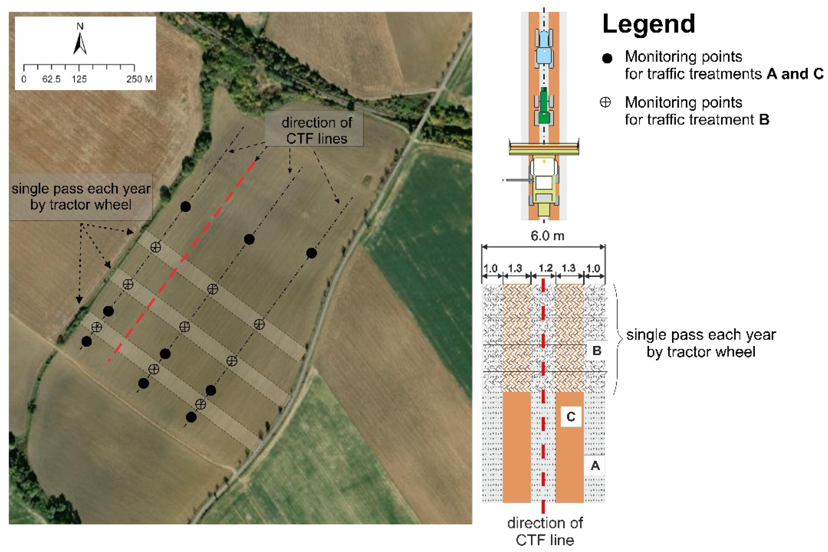
2.1. Experimental Field Characteristics

A long-term field scale experiment based on a 16 ha (48°37′17″ N, 18°20′75″ E) field converted to CTF together with soil conservation tillage was established in 2010. The CTF system was designed on the basis of a 6 m machinery module (Figure 1), resulting in 55% of the field being a no traffic area, 39% covered by a single pass (combine harvester), and 24% covered by permanent tramlines. The permanent tramlines were used for all field traffic, and thus they represent multiple traffic soil; their direction is shown in Figure 1. In order to obtain a larger area of single-pass traffic needed for sampling and analyses, three strips were trafficked by tractor wheel (single pass) each year (Figure 1). These areas were compacted by a wheeled tractor, which is also used for other field operations, during each year, after each harvest. The machinery traffic patterns and the layout of the experiment had been previously used [6,7]. Hereby, three different traffic intensity areas were found in the field, i.e., the soil with no traffic (soil which has not been subjected to the traffic of agricultural machinery since 2009), the soil with one traffic pass a year (RTF strips), and the soil with multiple traffic passes a year (permanent traffic lines).
For sampling and data collection, these refer to A, B, and C areas, where:
A is a no traffic area;
B is a single pass area;
C is a multiple pass/permanent tramline area.
In the long-term experiment, there are 9 locations in each area, i.e., A, B, and C, monitored in terms of yield and selected soil parameters since 2010 (Figure 1). However, these parameters were not the subject of this paper.
One location in each area, i.e., A, B, and C, was selected to conduct in situ measurements of soil erosion, as further explained in Section 2.2.
In terms of field management, before the CTF technology was implemented, a conventional plough was used. However, a soil conservation method based on crop residue distribution and shallow tillage has been used since 2009. Direct sowing (zero tillage) was implemented in the 2021 season. As this is a field scale experiment, the field was treated as a whole from an agronomic point of view: tillage and other crop operations were the same.
Field elevation varies between 196 and 212 m above sea level. The field exhibits a downward slope in the direction of east to west, which ranges between 3 and 7%. The soil texture was analysed on the basis of the Slovak Standards [26] and classified according to the Novak classification [27], being characterised as a silt loam (both the topsoil and subsoil). The only exception was the subsoil in the southwest corner, which has a slightly higher clay content than the rest of the field and, therefore, was characterised as a clay loam.

2.2. Field Measurements, Calculations, and Modelling

2.2.1. Soil Erosion Model

As it is not economically viable to carry out soil erosion measurements using a rain simulator in the whole field, one of the 9 locations for A, B, and C traffic intensity areas needed to be targeted. As the aim was to identify the field area having the highest erosion risk, the soil erosion was firstly modelled. The USLE (universal soil loss equation) model, which represents the average yearly soil erosion, was used, and defined as [28]
E = R × K × LS × C × P
where
  • E is the soil loss (t ha−1);
  • R is the rainfall erosivity (MJ mm ha–1);
  • K is the inherent erodibility of the soil (t ha−1 h ha–1 MJ–1 mm–1);
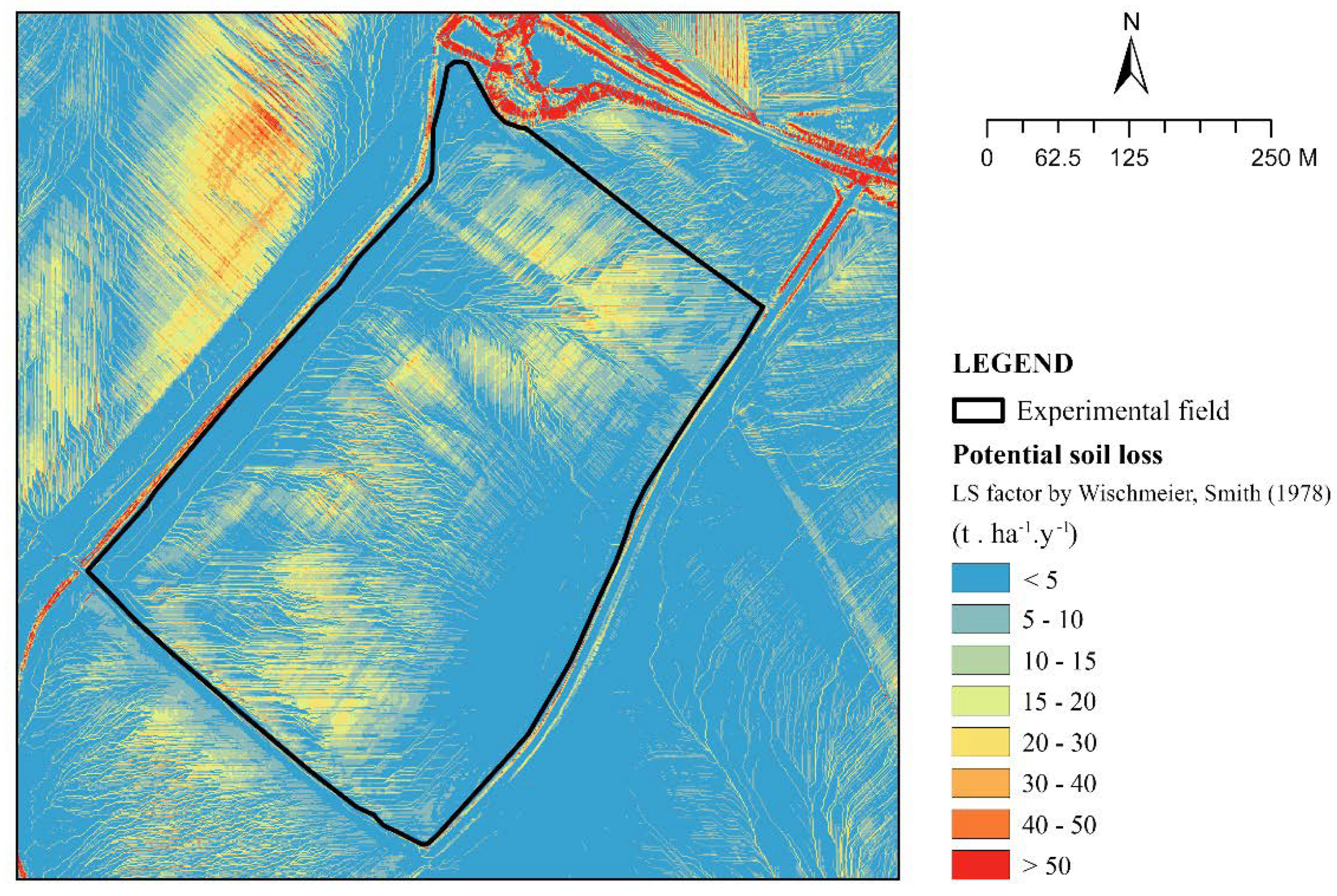
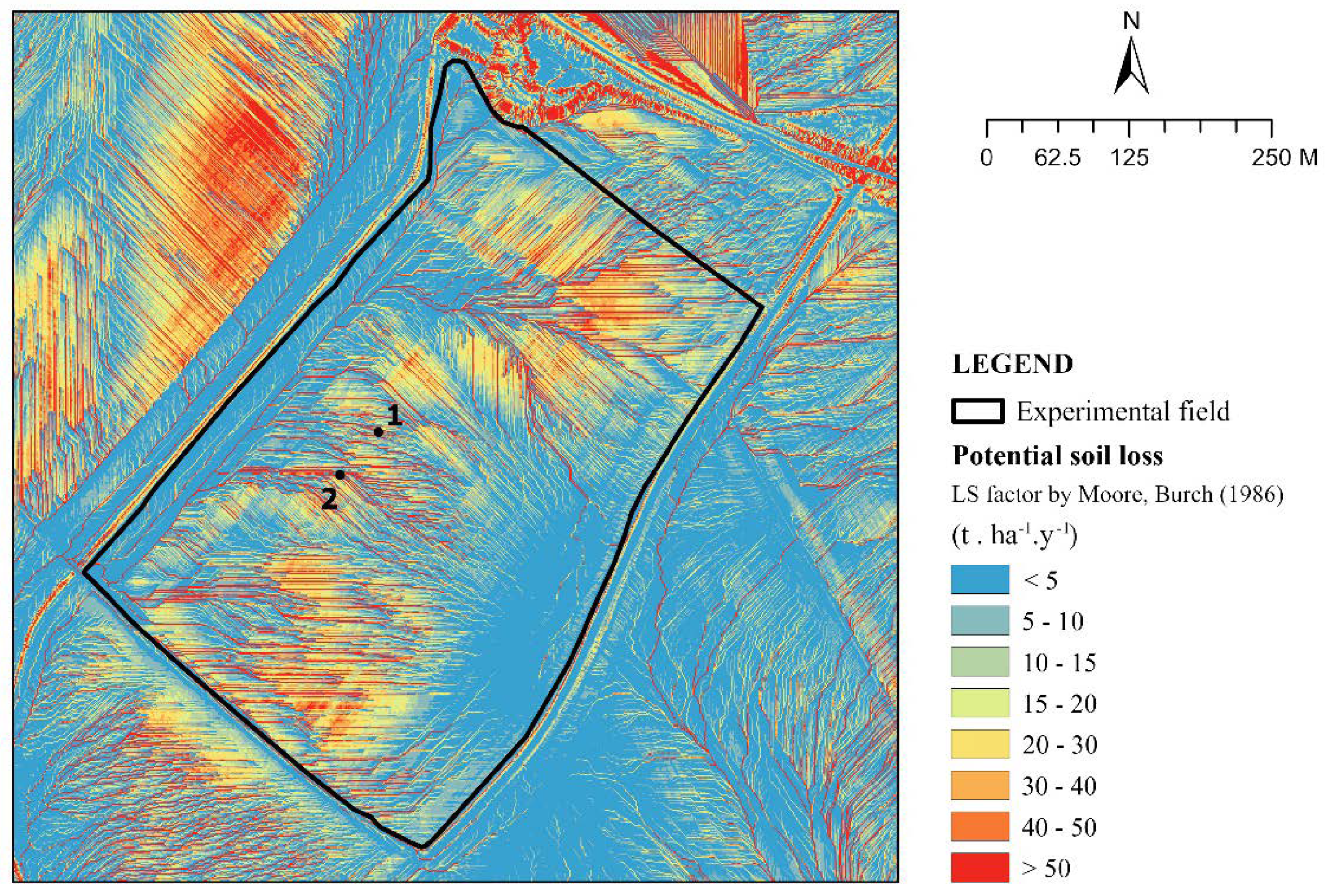
  • LS is a dimensionless topographic factor based on slope length and steepness (-);
  • C is a dimensionless factor representing vegetative cover (-);
  • P is a dimensionless conservation support practice factor (-).
The values of these erosion factors were determined from the long-term data of the total rainfall and its intensity (R-factor), the soil survey (K-factor), a high-resolution digital elevation model (LS-factor), the landscape structure (C-factor), and the land management (P-factor) were neglected as they would not affect the differences between the A, B, and C locations.
The evolution of USLE resulted in RUSLE (revised universal soil loss equation), derived by Moore and Burch [29] and applied by Desmet et al. [30] and Mitasova et al. [31]. This model includes a replacement of the slope length factor (L) (as a part of the topographic factor—LS), with 5 as the upslope contributing area (A), so that the model can predict an increased soil loss (by erosion) due to a concentrated flow, without the need to define these areas as individual inputs. The modified LS factor was calculated on the basis of the equation:
LS = Am × (sin β)n, (-)
where
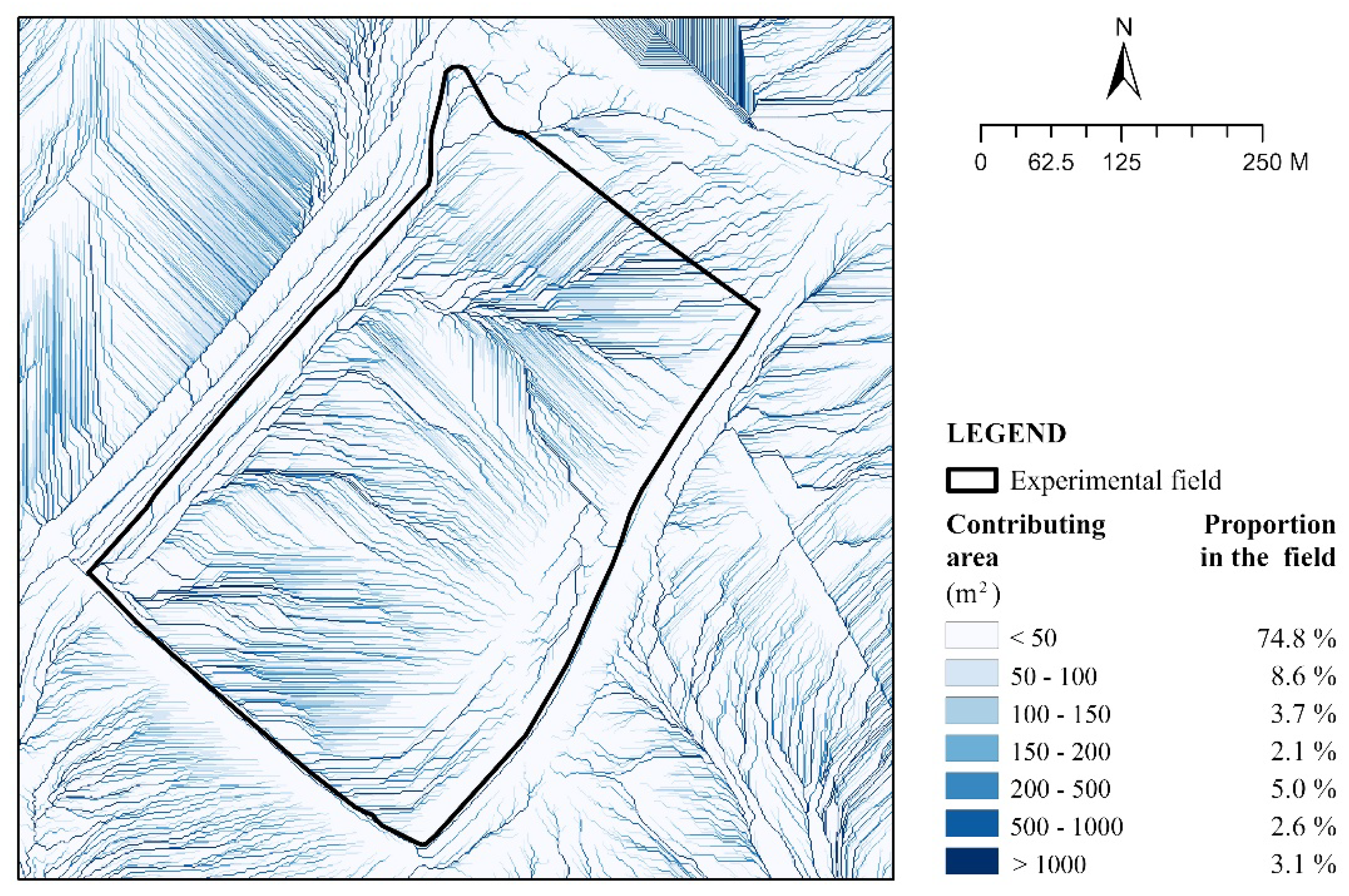
  • A is the upslope contributing area per width unit (m2 m−1);
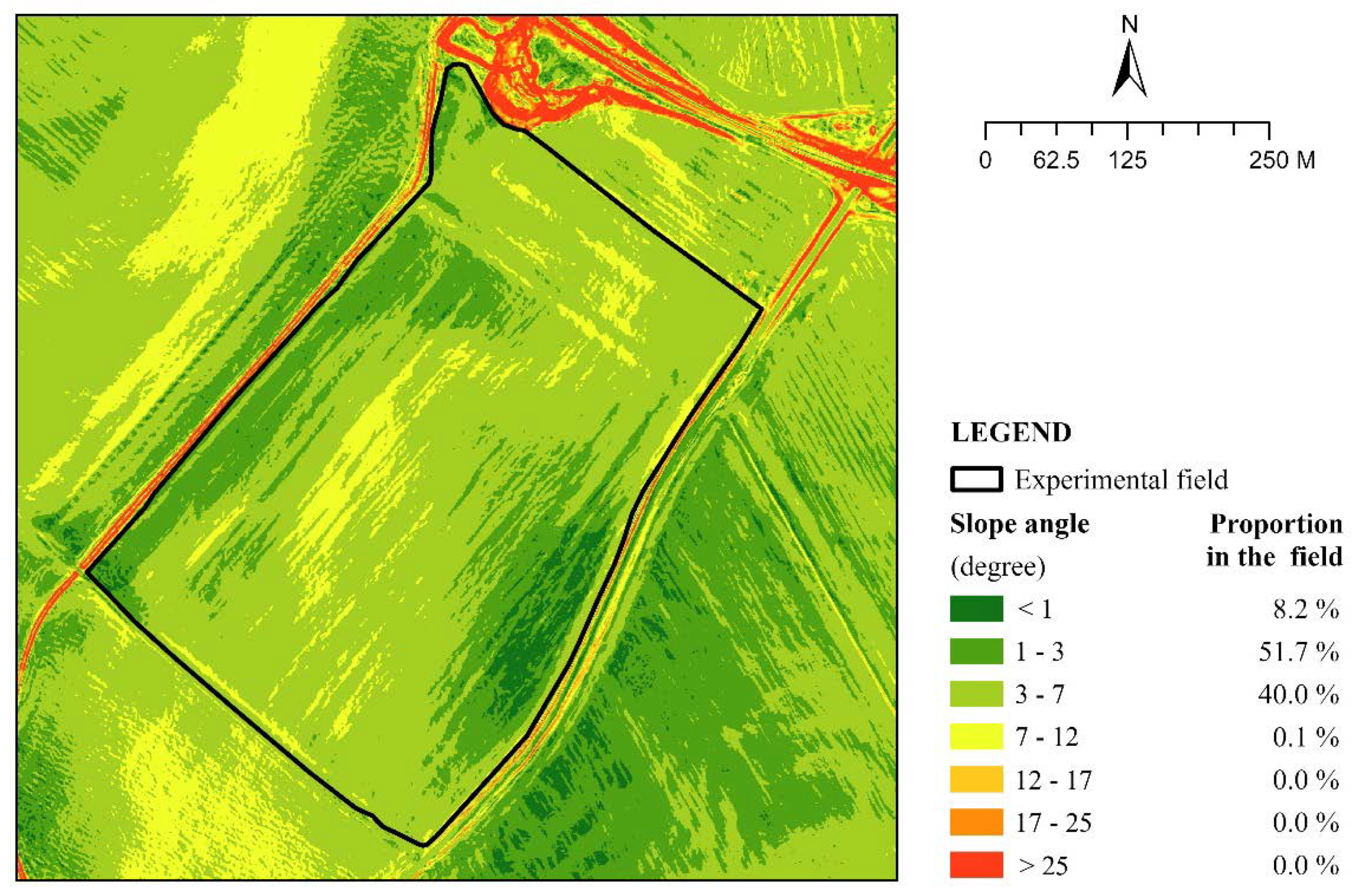
  • Β is the slope angle (°);
  • m and n are constants that depend on the type of flow and the soil parameters (-).
Where the rill soil erosion prevails, the constant values are usually defined as m = 1.6 and n = 1.3; where the sheet erosion dominates, they are set to m = n = 1.0 [32].
In order to process these models for the experimental area, the following data sources were used:
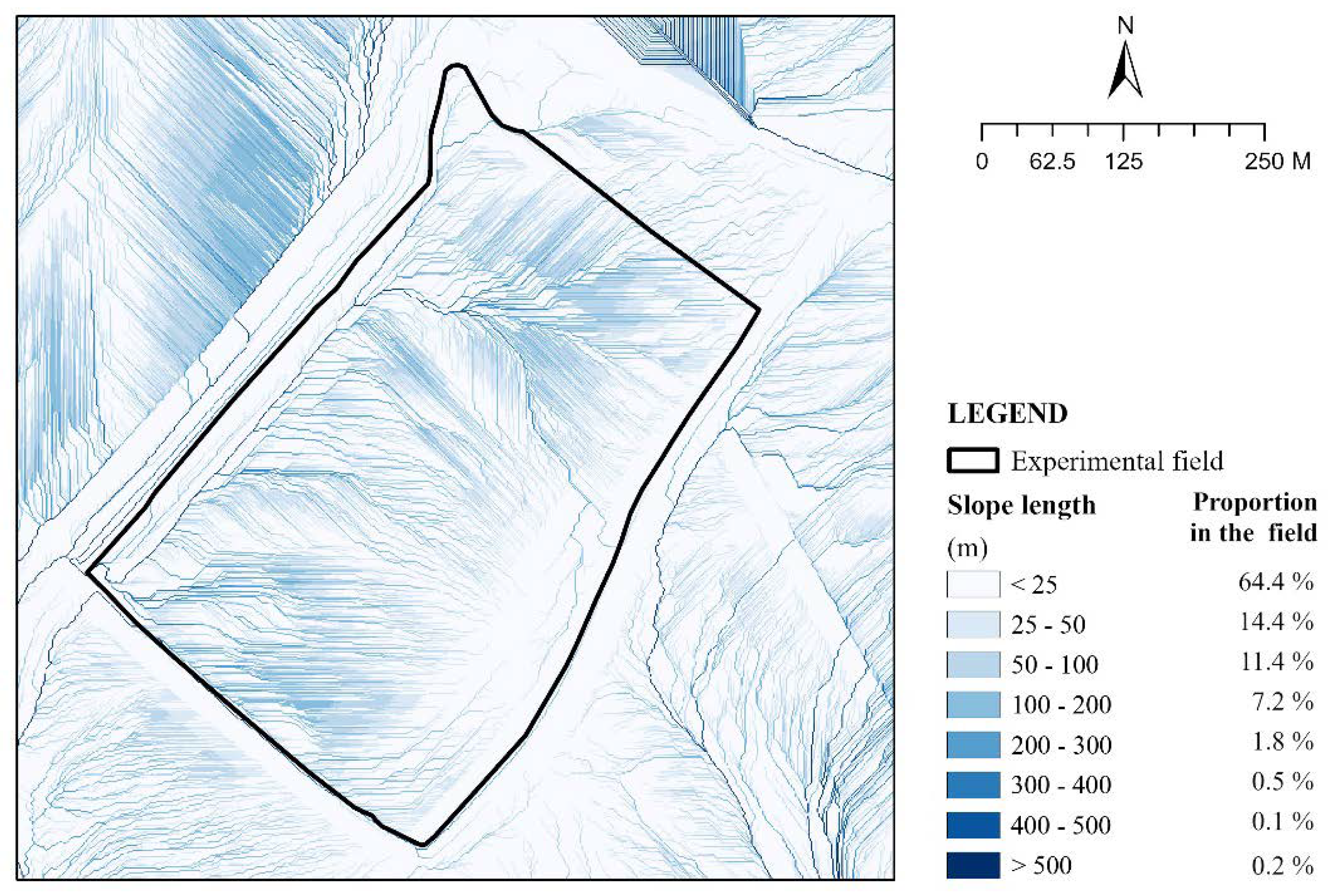
  • Digital Terrain Model 5.0 (DTM 5.0)—year 2018 (having a spatial resolution of 1 m), established in 2017 by the Geodesy, Cartography and Cadastre Authority of the Slovak Republic (ÚGKK SR) [33]; the output data from the airborne laser scanning (ALS) were used; they are characterised by the scanning density of 33 points per m2 and the absolute vertical accuracy of the point cloud of 0.03 m; the DTM 5.0, as a raster model having a spatial resolution of 1 × 1 m, was built up using the inverse distance weighting (IDW) interpolation method.
  • The flow direction (as an input raster for calculating the slope length and contributing area) was derived by the D8 algorithm [34].
Orthophotomosaic—year 2020 (having a spatial resolution of 0.20 m), provided by Geodetic and Cartographic Institute Bratislava (GKÚ) and National Forest Centre (NLC) [35]. The R-factor was determined according to the nearest precipitation gauge station (Nitra) as a constant value (24.62) from the published data [36]. The value was obtained by evaluating rainfall records for a 50-year observation period (since 1960). As the rain intensity changes during a rainstorm, the rainfall curves were divided into sections having approximately the same intensity, while the kinetic energy was calculated for each section. As Slovakia is located at the border of inland continental and coastal climates in variable weather conditions, thus rainstorms vary in intensity; for this reason, published rainfall records were used. The K-factor was defined according to the main soil unit in the experimental field, as well as a constant value (0.59) from the available source [37]. The determination of the value was preceded by a soil analysis performed by the Soil Science and Conservation Research Institute (SSCRI) in Bratislava between 1960 and 1970. The soil sample was taken from a depth of 20 cm. The current research from 2010 did not find any significant differences in the soil properties measured. On the basis of the calculated models, the locations for the in situ measurement of water runoff and soil loss were targeted. The details of these measurements are provided in Section 2.2.2.

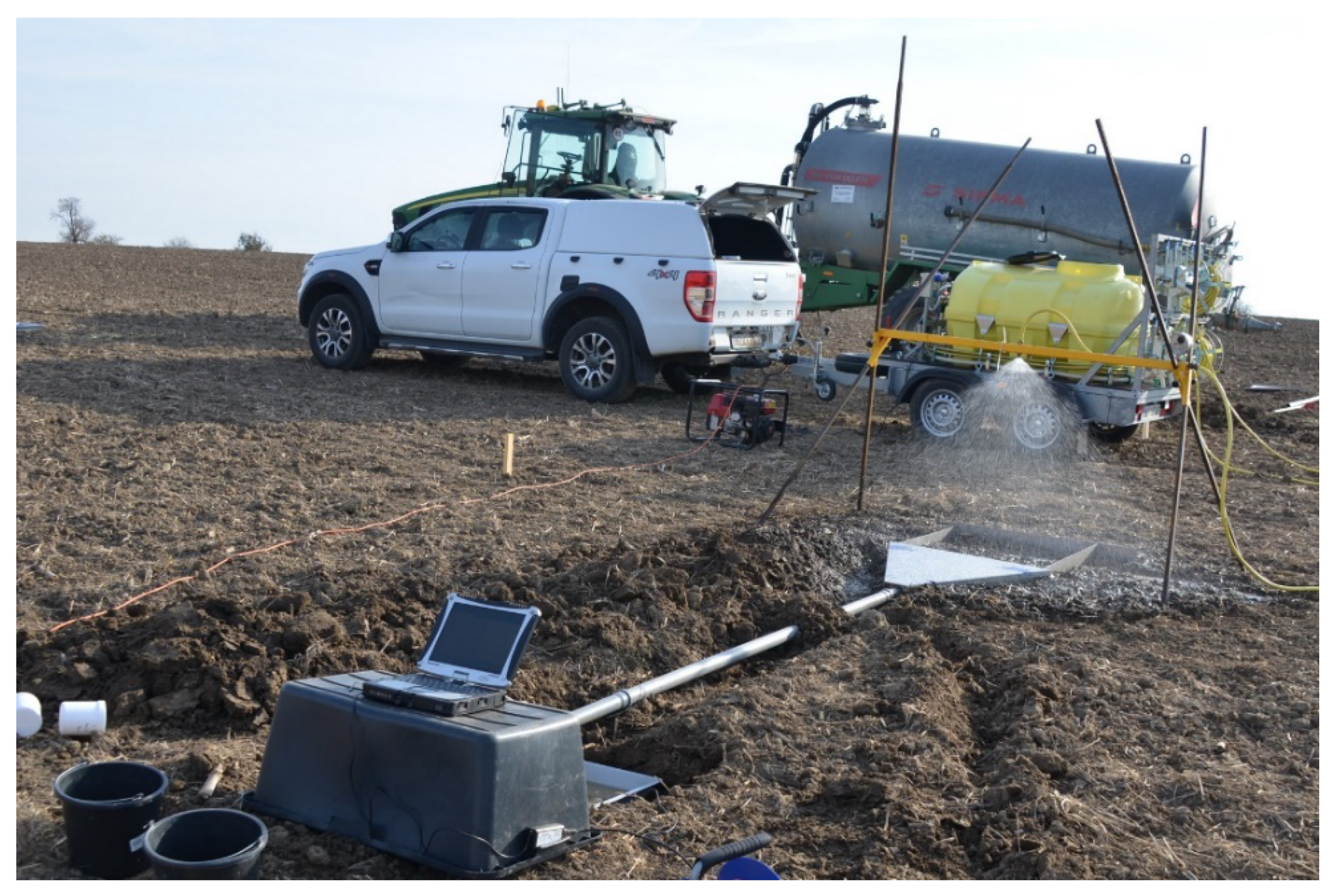
2.2.2. Field Measurements of Water Runoff and Soil Rainfall Loss

The soil erosion measurements were conducted in October 2021. The climate characteristics of the year are shown in Table 1 and Figure 2. In order to show the actual water regime conditions of the field, the actual soil moisture was determined following the same methodology described in Section 2.2.2.
On the basis of the soil erosion model (Section 3.2), the field area with the highest erosion risk was targeted. Within this area, three locations were selected to reflect the three different traffic intensities (A, B, and C) where the rainfall simulator assessments took place.
The rainfall simulator (Figure 3) was designed at the Czech University of Life Sciences in Prague [38] and consisted of a frame which could sprinkle a selected amount of water above the soil surface 1 m above the ground. The water which ran off the area of 0.5 m2 was collected and continuously weighted. Hereby, the water runoff from the area was determined every minute and interpreted as the water runoff intensity. The water was analysed in the laboratory. The collected soil sediments were dried and then weighted. Hereby, the soil loss caused by rain erosion was determined.
The measurements were conducted in the 3 locations with 4 replications (2 in each monitoring point). The rain intensity of 1.3 mL min−1 was simulated for 50 min, which is equal to the rainfall of 80 mm per hour.

2.2.3. Soil Compaction Measurements

In order to complete the information on the locations, soil compaction was measured in the study locations. The handheld soil cone penetrometer Eijlkelkamp 06.15.31.SA, having an accuracy of ±0.01 MPa (eijlkelkamp.com, accessed on 20 October 2022), was used during the tests. Soil cone penetrometer resistance was measured and recorded every centimetre until the depth of 80 cm. A cone tip having a bottom area of 1 cm2 and a vertex angle of 60° was used, according to the ASABE standard S313.3 [36]. In each location (A, B, and C), 45 replications were obtained. The sampling methodology followed the ASABE standard EP542.1 [39,40]. The actual soil moisture was measured at the same time using the gravimetric method following the standard ISO 11465 [41].
The statistical analysis was performed for all traffic treatments using Statistica software [42]. This analysis involved tests of normality (Shapiro–Wilk test), descriptive statistics followed by Levene’s test of variance homogeneity, and the analysis of variance (ANOVA) and least significant differences (LSD), in order to compare the means using probability levels of 5%.

3. Results

3.1. Soil Erosion Model of the Field

In order to calculate the erosion model, the slope length was firstly analysed (Figure 4). The slope length was lower than 25 m in 64.4% of the experimental area. However, there were some extreme lengths—the longest one was 700 m. As shown in Figure 4, the longest slope went from north to east, downhill, and along the western border. Moreover, it was clear that the field area was affected by the surrounding fields, as there was water coming from the other areas, especially the neighbouring area to the north. For the calculations of RUSLE, the contributing area was needed, as shown in Figure 5. Most of the field had a contributing area lower than 50 m2.
The slope angle of the land ranged from less than 1° to 12°.
It was evident that the middle part of the field was the steepest one, ranging from 3 to 7° (Figure 6).
On the basis of the above information, the potential yearly soil loss was calculated according to USLE, as well as its modification (RUSLE). The data are shown in Figure 7 and Figure 8. The highest risk of soil erosion causing the highest soil loss was identified on the steep areas. The areas which had different categories of soil loss risk are shown in Table 2. According to both calculations, the potential yearly soil loss ranged from less than 5 to 50 t ha−1. Even if most of the area of the experimental field had the lowest potential yearly soil loss, a yearly soil loss between 5 and 15 t ha−1 was found in almost 30% of the area itself.
As shown in Figure 7 and Figure 8, the D8 algorithm used to derive the flow direction caused a dense concentration in the outflow paths. Due to the high quality of the used data, the resampling the DTM grid with a cell size of 1 × 1 m to 5 × 5 m or 10 × 10 m spatial resolution was not viable. Indeed, such a change would reduce the density of water runoff concentration but degrade the quality of input data. As part of further research, a focus on the use of multiple flow direction (MFD) algorithms, such as the MD8 algorithm, is required. Alternatively, applying filters (i.e., generalisation) for the purpose of “editing” DTM 5.0 can be recommended for the needs of erosion–hydrological analyses.

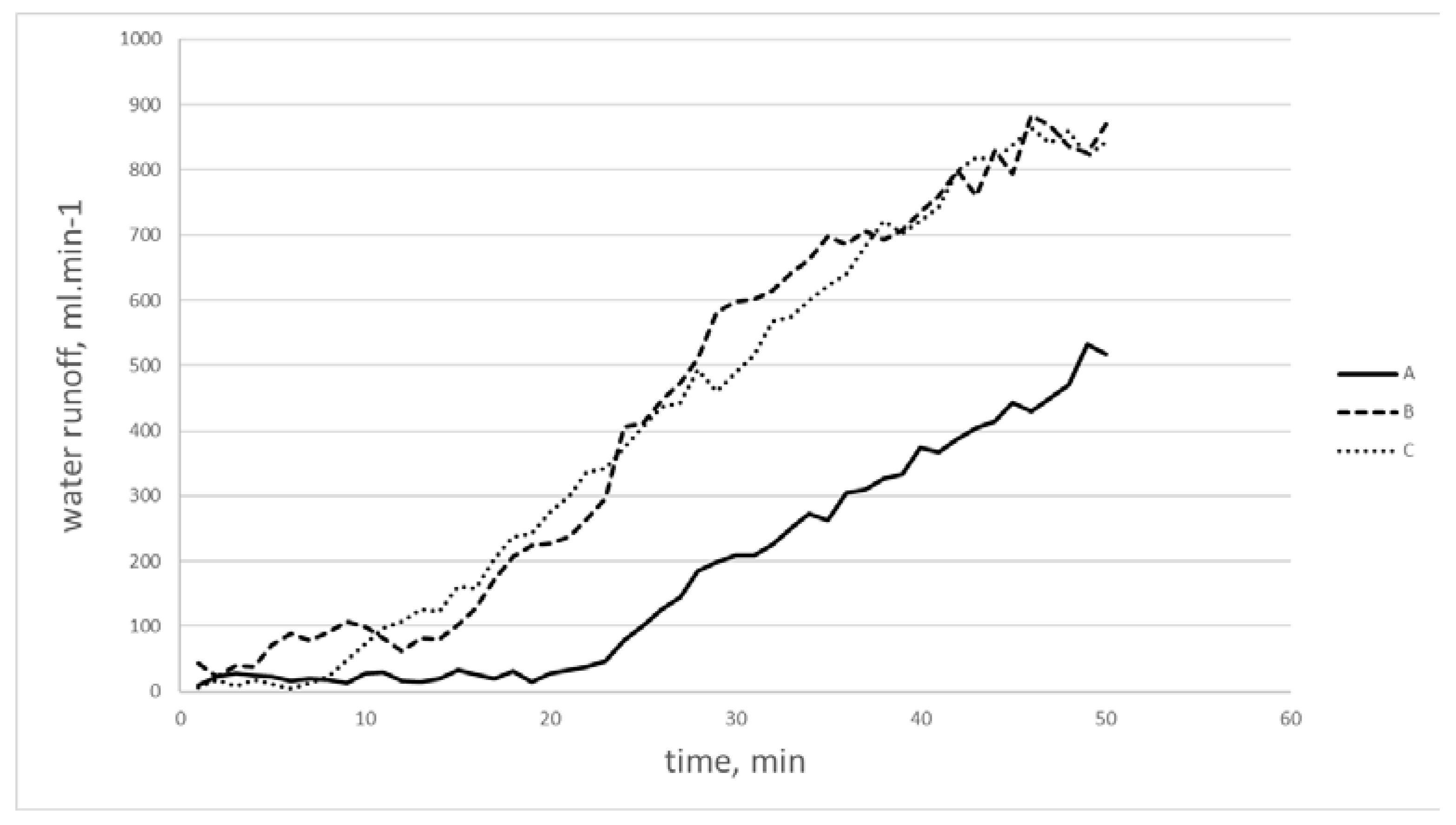
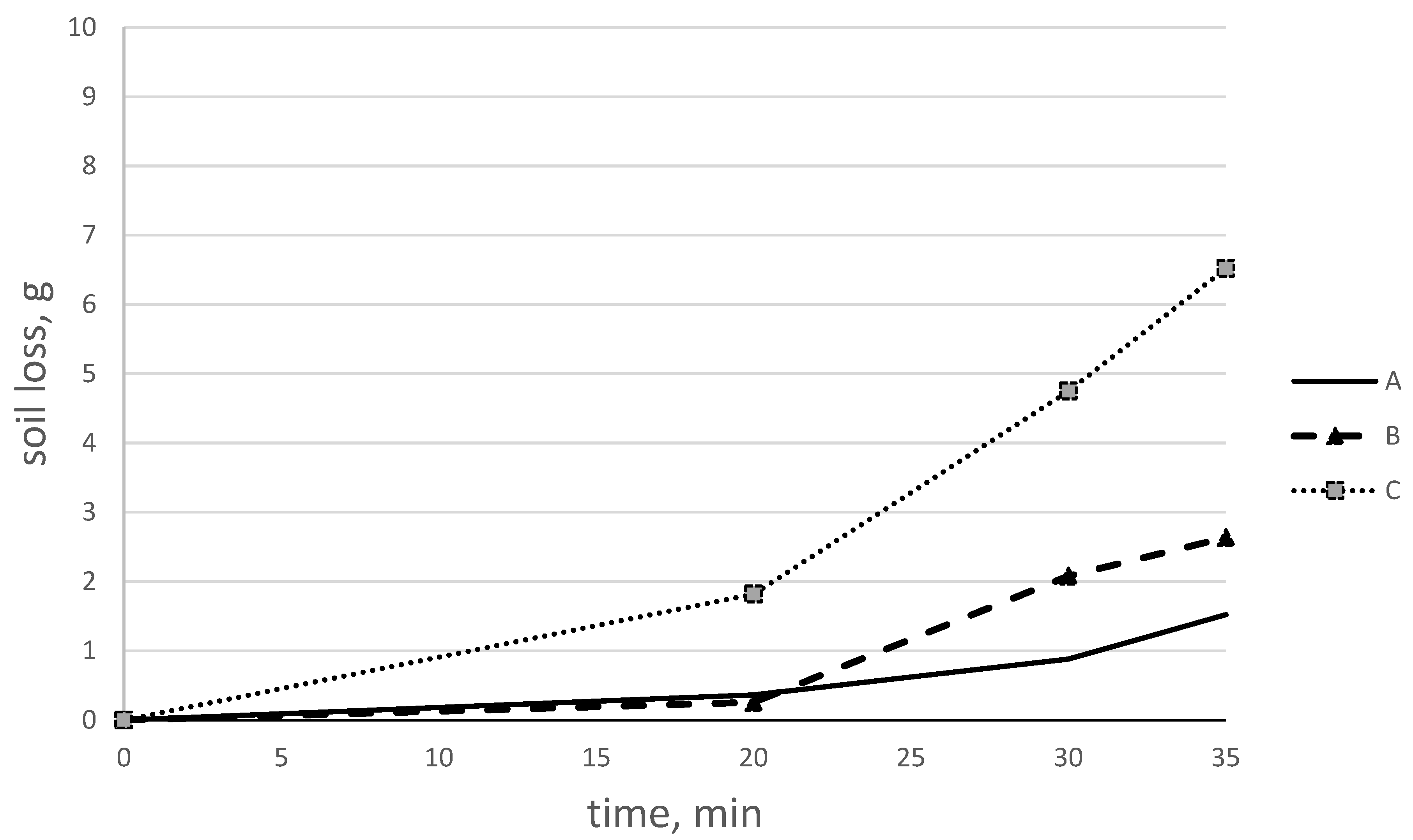
3.2. Calculation of Water Runoff and Soil Loss

On the basis of the erosion model derived from the available data, the field areas with the highest erosion risk were targeted. These areas are shown in Figure 8 as sites 1 and 2. In site 1, the rainfall simulator was used for measurements in location B, while in site 2, the locations A and C were targeted. The distance between A and C is shown in Figure 1.
The soil moisture content was measured before the rain simulation. The average soil moisture content was 22.14%, which indicates dry conditions, according to the climate parameters and calculated soil water limits shown in Table 3. This was also expected from the climate conditions of the year, which are shown in Figure 2.
The water runoff from the three locations (A, B, and C) is shown in Figure 9. The data show the amount of water which did not infiltrate into the soil from the applied amount (1300 mL min−1). In location A, almost all the water infiltrated within the first 20 min. Then, the water runoff started to increase, and after 50 min, it increased to 500 mL min−1. In location B, the water runoff started to increase after 15 min. In location C, the lowest infiltration and, consequently, the highest runoff were reached: the water started to flow on the soil surface 8 min after the simulated rain. For both compacted locations (single and multiple passes), the water which exceeded the infiltration rate and resulted in runoff exceeded the values of 800 mL min−1 50 min after the simulated rain.
Further, the dry weight of sediments was derived in laboratory conditions. Due to the operational circumstances during the measurements, the samples were not taken in the same minute of rainfall simulation in all three locations, and thus the timescale differed for the A, B, and C locations. Figure 10 shows the soil loss (sediment weight) measured in each location. The total weight of sediments was determined after 35 min and resulted in being 1.52 g in location A, 2.63 g in location B, and 6.52 g in location C.

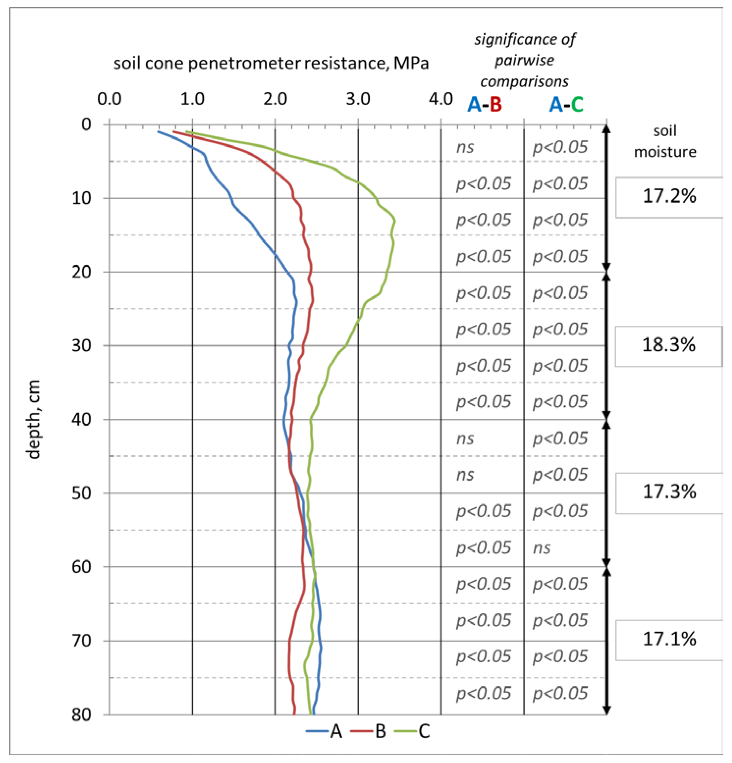
3.3. Determination of Soil Physical Parameters

In order to show the effect of using the permanent tramlines and avoiding soil compaction in the rest of the field, soil cone penetrometer resistance was measured in the three locations (Figure 11).
Soil moisture content was measured at three depths and ranged between 17.2 and 18.3%. The results confirmed that avoiding soil compaction significantly improved its structure in the topsoil, as it was expressed by significantly lower soil cone penetrometer resistance in location A, compared to locations B and C. In location C, the soil cone penetrometer resistance at the depth between 10 and 25 cm increased from 1.8 MPa, measured in location A, to 3.4 MPa. The subsoil conditions showed the effect of permanent tramlines, as location C was the most compacted area.

4. Discussion

Nowadays, in the conditions of climatic extremes, it is possible to observe more commonly occurring dry periods followed by heavy rainfalls in the continental climate. Even if GHG emissions, water restoration, and soil erosion have previously been investigated [1,14,19,21,43,44], the research on soil erosion itself is limited. Soil conservation methods include minimum or no tillage and soil coverage with crop residues [45]. Controlled traffic farming (CTF) increases these environmental benefits so that machinery traffic is confined to the least possible area (permanent tramlines), while the rest of the field is not compacted [45]. This study presents the benefits of CTF in terms of reduction in water erosion and soil loss. The long-term experiment, where CTF was implemented in 16 ha steep field, provides a unique experimental area. The layout of the experiment offered three areas with different traffic intensity: (A) no traffic; (B) single pass a year; (C) multiple passes/permanent tramlines a year.
In terms of soil erosion assessment, the experimental field was evaluated firstly as the whole 16 ha area, using the data from the long-term research. The erosion risk was determined by means of USLE and its revised version (RUSLE) using the LS factor, providing the potential yearly soil loss. Both approaches showed that almost 30% of the field had the erosion risk of 5–15 t ha−1, which is within the maximum value established by Slovak legislation, i.e., 15 t ha−1 [46]. On the basis of the compensation theory of soil erosion [47], the yearly soil gain was estimated to be 1.5 t ha−1.
Then, the area of highest erosion risk was targeted. Here, a series of in situ field measurements of water runoff and, consequently, soil loss was carried out in the three areas with different traffic intensities. Rain intensity of 1300 mL min−1 was simulated to evaluate the intensity of water runoff recorded in the locations after 20 and 40 min. In location A, almost all water infiltrated into the soil after the first 20 min. The water runoff intensity of 28 mm min−1 was recorded after 20 min. After another 20 min (40 min after the beginning of rain simulation), the water runoff intensity of 374 mL min−1 was recorded. In location B, with one machinery pass a year, after 15 min, the water runoff started to increase up to 227 mL min−1 after 20 min and further to 721 mL min−1 after 40 min. In location C, water runoff started to increase after 8 min, while after 20 min, its intensity reached the value of 276 mm min−1, and after 40 min, 722 mL min−1. It is evident that the soil subjected to the multiple forms of traffic of agricultural machinery reached the highest rates of runoff and the water started to flow on the surface earlier after the rain simulation.
These results are in agreement with the research conducted in the UK and Australia [21,48,49] and can be explained by damaged soil structure caused by heavy agriculture machinery passes [50]. The direction of permanent traffic lines (location C) is important to manage water runoff [16]. In the experimental field, the permanent tramlines were designed perpendicular to the slope, as this is the best practice of crop establishment used in Slovakia. However, some scientists [13] report that, when the permanent traffic lines are parallel to the slope, the water runoff is better stimulated.
Moreover, the infiltration rates can be determined from the obtained data when the water that runs off is subtracted from the applied water. The improved soil infiltration in location A results from the improved soil structure, compared to locations B and C. These results are consistent with others published on the improved infiltration rate [48,49,51]. The improved soil structure is proved by the soil cone penetrometer resistance measurements. The differences in the topsoil were statistically significant at p lower than 0.05. The highest difference between the locations A and C was at the depth of 15 cm, while the soil cone penetrometer resistance in location C was double the value in location A. The effect of the soil compaction caused by agriculture machinery was evident also in the subsoil (30–80 cm), where the highest soil cone penetrometer resistance was obtained after multiple passes (area C). Although the differences were lower than in the topsoil, they were still statistically significant (p < 0.05). Some studies reported that the stress from agricultural machinery is transferred down to 1 m depth [52].
The water samples collected in the three locations showed that one machinery pass a year caused an increase in water runoff by 50%, compared to no traffic soil. After multiple traffic passes, the area can lose almost triple its amount of water when compared to no traffic soil. Assessing the soil sediments in the water samples showed that in location B, 73% more sediments were found after 35 min of simulated rain, compared to location A. The soil compacted by multiple machinery passes (location C) recorded the worst results, i.e., 6.52 g of soil in the sample collected after 35 min, compared to 1.52 g in the location without any traffic applied for 12 years. The area which has the potential to benefit from better infiltration, lower water runoff, and soil loss differs on the basis of the adopted CTF system. The ratio of the areas with different traffic intensity differs depending on machinery width, tyre contact area, and traffic scheme in the field. In random traffic farming (RTF) systems, machinery can apply their weight to up to 88% of the field a year if ploughing is implemented. This area decreases to 73 and 56% for the field if minimum or no tillage (direct sowing) is implemented, respectively [3]. On the contrary, CTF systems used in Australia result in 85% of their area not being subjected to the traffic of agricultural machinery [8]. In Europe, different CTF systems are used, and the best system for reducing the area subjected to the traffic of agricultural machinery is based on an 8 m machinery module. When permanent traffic lines are used and 8 m wide machines are matched, 77% of the field is not subjected to traffic. Environmental and economic benefits can, then, be extrapolated on the basis of this ratio. A yield increase of 4% was recorded for a CTF system with a 30% traffic area, while a further improvement up to 7% yield was obtained for a CTF system with 15% of traffic soil [14].
The practical adoption of CTF in Europe follows the “tier” approach [48], beginning with low-cost conversion from RTF to CTF, on the basis of using standard farm machinery and respecting only the CTF layout (as is the case of the presented experimental site) up to the 8 m module, where machinery replacement would be needed. Therefore, the cost of technology implementation may vary from investments for only GNSS technology to those for tractor adjustments and implement replacement. However, these initial costs are compensated by the economic benefits derived from increased crop yields and decreased tillage costs, as shown by Godwin et al. [14] and Galambosova [53], who confirmed that even the most expensive conversion to an 8 m module would pay off within 4 years for an area of 500 ha, 2.5 years for 1000 ha, and within 1.5 years for 2000 ha [53].
However, the aim of this work was to show that the permanent reduction of field traffic significantly reduces the soil loss caused by water runoff, which is economically unmeasurable.

5. Conclusions

This work evaluated the effect of a controlled traffic farming (CTF) system (in field conditions) on water runoff and soil erosion, estimated using the USLE equation. The results showed that up to 30% of the field has a potential yearly soil loss of 5 to 15 t ha−1.
Furthermore, three areas with different traffic intensity were used to conduct a series of measurements by means of a rain simulator. The area where no traffic has been applied for 12 years (location A) showed significantly better conditions in terms of soil structure, which was reflected in the lower water runoff and soil loss. When comparing the data 35 min after rain simulation with an intensity of 1300 mL min−1, the following results were obtained:
-
the water runoff intensity was on average 2.5 times lower in the no traffic area (A), compared to the traffic areas (B and C);
-
the amount of total water and sediments collected after 35 min increased by 50% in the area with one machinery pass (B), compared to the A area; in the multiple traffic area (C), it tripled, compared to the no traffic area (A);
-
the weight of soil loss, expressed in terms of soil sediments, was 1.7 times higher in one machinery pass area (B) and 4.3 times higher in multiple pass area (C), compared to the no traffic area (A).
The results show that CTF offers the potential to significantly reduce water erosion and soil loss on steep land.

Author Contributions

Conceptualisation, J.G. and M.M.; methodology, J.G., M.K., F.K., M.M. and K.Š.; software, K.Š.; validation, J.G., M.M. and F.K.; formal analysis, K.Š., J.G. and M.M.; investigation, M.M., M.B., F.K., V.R. and P.N.; resources, M.M. and V.R.; data curation, M.K., M.B., F.K., K.Š. and M.M.; writing—original draft preparation, J.G.; writing—review and editing, P.A.M. and M.M.; visualisation, K.Š. and M.M.; supervision, J.G. and M.M.; project administration, V.R.; funding acquisition, V.R., M.M. and J.G. All authors have read and agreed to the published version of the manuscript.

Funding

This publication is the result of the project implementation “Scientific support of climate change adaptation in agriculture and mitigation of soil degradation” (ITMS2014 + 313011W580), supported by the Integrated Infrastructure Operational Programme funded by the European Regional Development Fund (ERDF). This publication was supported by the Operational Programme Integrated Infrastructure within the project “Sustainable smart farming systems taking into account the future challenges” (313011W112), co-financed by the European Regional Development Fund (ERDF). This publication was supported by the Grant Agency of Slovak University of Agriculture in Nitra, Slovakia, within the project “Effect of controlled traffic farming technology on water erosion of soil” (GA-SPU 28/2019).

Institutional Review Board Statement

This study did not require ethical approval.

Informed Consent Statement

This study did not involve humans.

Data Availability Statement

This study did not report any data.

Acknowledgments

The authors are grateful to the staff of the University Farm in Kolinany, Slovakia, for their technical and operational support during this research.

Conflicts of Interest

The authors declare no conflict of interest.

References

  1. Antille, D.L.; Peets, S.; Galambošová, J.; Botta, G.F.; Rataj, V.; Macák, M.; Tullberg, J.N.; Chamen, W.C.T.; White, D.R.; Misiewicz, P.A.; et al. Review: Soil compaction and controlled traffic farming in arable and grass cropping systems. Agron. Res. 2019, 17, 653–682. [Google Scholar] [CrossRef]
  2. Chamen, W.C.T.; Moxey, A.P.; Towers, W.; Balana, B.; Hallett, P.D. Mitigating arable soil compaction: A review and analysis of arable cost and benefit data. Soil Tillage Res. 2015, 146, 10–25. [Google Scholar] [CrossRef]
  3. Kroulík, M.; Kumhála, F.; Hůla, J.; Honzík, I. The evaluation of agricultural machines field trafficking intensity for different soil tillage technologies. Soil Tillage Res. 2009, 105, 171–175. [Google Scholar] [CrossRef]
  4. Tullberg, J.N. Tillage, traffic and sustainability—A challenge for ISTRO. Soil Tillage Res. 2010, 111, 26–32. [Google Scholar] [CrossRef]
  5. Chamen, T. Controlled traffic farming—From worldwide research to adoption in Europe and its future prospects. Acta Technol. Agric. 2015, 3, 64–73. [Google Scholar] [CrossRef] [Green Version]
  6. Rataj, V.; Kumhálová, J.; Macák, M.; Barát, M.; Galambošová, J.; Chyba, J.; Kumhála, F. Long-Term Monitoring of Different Field Traffic Management Practices in Cereals Production with Support of Satellite Images and Yield Data in Context of Climate Change. Agronomy 2022, 12, 128. [Google Scholar] [CrossRef]
  7. Galambošová, J.; Macák, M.; Rataj, V.; Antille, D.L.; Godwin, R.J.; Chamen, W.C.T.; Žitňák, M.; Vitázková, B.; Ďuďák, J.; Chlpík, J. Field evaluation of controlled traffic farming in central Europe using commercially available machinery. Trans. ASABE 2017, 60, 657–669. [Google Scholar] [CrossRef]
  8. Vermeulen, G.D.; Mosquera, J. Soil, crop and emission responses to seasonal-controlled traffic in organic vegetable farming on loam soil. Soil Tillage Res. 2009, 102, 126–134. [Google Scholar] [CrossRef]
  9. Torbert, H.A.; Wood, C.W. Effects of soil compaction and water-filled pore space on soil microbial activity and N losses. Commun. Soil Sci. Plant Anal. 1992, 23, 1321–1331. [Google Scholar] [CrossRef]
  10. Antille, D.L.; Chamen, W.C.T.; Tullberg, J.N.; Lal, R. The potential of controlled traffic farming to mitigate greenhouse gas emissions and enhance carbon sequestration in arable land: A critical review. Trans. ASABE 2015, 58, 707–731. [Google Scholar] [CrossRef]
  11. Tullberg, J.N.; Yule, D.F.; McGarry, D. Controlled traffic farming: From research to adoption in Australia. Soil Tillage Res. 2007, 97, 272–281. [Google Scholar] [CrossRef]
  12. Puccio, D.; Comparetti, A.; Greco, C.; Raimondi, S. Proposal of a Nomenclature for Hydrogeological Instability Risks and Case Studies of Conservative Soil Tillage for Environmental Protection. Land 2022, 11, 108. [Google Scholar] [CrossRef]
  13. Soane, B.D.; Ball, B.C.; Arvidsson, J.; Basch, G.; Moreno, F.; Roger-Estrade, J. No-till in northern, western and south-western Europe: A review of problems and opportunities for crop production and the environment. Soil Tillage Res. 2012, 118, 66–87. [Google Scholar] [CrossRef] [Green Version]
  14. Godwin, R.J.; White, D.R.; Dickin, E.T.; Kaczorowska-Dolowy, M.; Millington, W.A.J.; Pope, E.K.; Misiewicz, P.A. The effects of traffic management systems on the yield and economics of crops grown in deep, shallow and zero tilled sandy loam soil over eight years. Soil Tillage Res. 2022, 223, 105465. [Google Scholar] [CrossRef]
  15. Panagos, P.; Imeson, A.; Meusburger, K.; Borrelli, P.; Poesen, J.; Alewell, C. Soil Conservation in Europe: Wish or Reality? Land Degrad. Dev. 2016, 27, 1547–1551. [Google Scholar] [CrossRef] [Green Version]
  16. Gasso, V.; Sørensen, C.A.G.; Oudshoorn, F.W.; Green, O. Controlled traffic farming: A review of the environmental impacts. Eur. J. Agron. 2013, 48, 66–73. [Google Scholar] [CrossRef]
  17. Tullberg, J.; Antille, D.L.; Bluett, C.; Eberhard, J.; Scheer, C. Controlled traffic farming effects on soil emissions of nitrous oxide and methane. Soil Tillage Res. 2018, 176, 18–25. [Google Scholar] [CrossRef]
  18. Hussein, M.A.; Antille, D.L.; Kodur, S.; Chen, G.; Tullberg, J.N. Controlled traffic farming effects on productivity of grain sorghum, rainfall and fertiliser nitrogen use efficiency. J. Agric. Food Res. 2021, 3, 100111. [Google Scholar] [CrossRef]
  19. Novara, A.; Novara, A.; Comparetti, A.; Santoro, A.; Cerdà, A.; Rodrigo-Comino, J.; Gristina, L. Effect of Standard Disk Plough on Soil Translocation in Sloping Sicilian Vineyards. Land 2022, 11, 148. [Google Scholar] [CrossRef]
  20. Tullberg, J.N.; Ziebarth, P.J.; Yuxia, L. Tillage and traffic effects on runoff. Aust. J. Soil Res. 2001, 39, 249–257. [Google Scholar] [CrossRef]
  21. Li, Y.X.; Tullberg, J.N.; Freebairn, D.M. Wheel traffic and tillage effects on runoff and crop yield. Soil Tillage Res. 2007, 97, 282–292. [Google Scholar] [CrossRef]
  22. Wang, X.Y.; Gao, H.W.; Tullberg, J.N.; Li, H.W.; Kuhn, N.; Mchugh, A.D.; Li, Y.X. Traffic and tillage effects on runoff and soil loss on the Loess Plateau of northern China. Aust. J. Soil Res. 2008, 46, 667–675. [Google Scholar] [CrossRef]
  23. Titmarsh, G.; Wockner, G.; Waters, D. Controlled traffic farming and soil erosion considerations. In Proceedings of the ISCO 2004- 13 th International Soil Conservation Organisation Conference, Brisbane, Australia, 4–8 July 2004; Conserving Soil and Water for Society: Sharing Solutions. Available online: https://www.tucson.ars.ag.gov/isco/isco13/PAPERS%20R-Z/TITMARSH.pdf (accessed on 11 November 2022).
  24. Boulal, H.; Gómez-Macpherson, H.; Gómez, J.A.; Mateos, L. Effect of soil management and traffic on soil erosion in irrigated annual crops. Soil Tillage Res. 2011, 115–116, 62–70. [Google Scholar] [CrossRef]
  25. McHugh, A.D.; Tullberg, J.N.; Freebairn, D.M. Controlled traffic farming restores soil structure. Soil Tillage Res. 2009, 104, 164–172. [Google Scholar] [CrossRef]
  26. Hrivňáková, K.; Makovníková, J.; Barančíková, G.; Bezák, P.; Bezáková, Z.; Dodok, R.; Grečo, V.; Chlpík, J.; Kobza, J.; Lištjak, M.; et al. Unified Analytical Procedures for Soil (Jednotné Pracovné Postupy Rozborov Pôd), 1st ed.; Soil Science and Conservation Research Institute (Výskumný Ústav Pôdoznalectva A Ochrany Pôdy): Bratislava, Slovakia, 2011; p. 136. ISBN 978-80-89128-89-1. [Google Scholar]
  27. Hraško, J.; Červenka, L.; Facek, Z.; Komár, J.; Němeček, J.; Pospíšil, F.; Sirový, V. Methods for Soil Analyses (Rozbory Pôd), 1st ed.; Slovenské Vydavateľstvo Pôdohospodárskej Literatúry: Bratislava, Slovakia, 1962; p. 342. ISBN 64-028-62 04-17. [Google Scholar]
  28. Wischmeier, W.H.; Smith, D.D. Predicting Rainfall Erosion Losses—A Guide to Conservation Planning (Agriculture Handbook Number 537), 1st ed.; Science and Education Administration of U.S. Department of Agriculture: Washington, DC, USA, 1978; p. 60. Available online: https://naldc.nal.usda.gov/download/CAT79706928/PDF (accessed on 18 October 2022).
  29. Moore, I.D.; Burch. G. Physical basis of the length-slope factor in the Universal Soil Loss Equation. Soil Sci. Soc. Am. J. 1986, 50, 1294–1298. [Google Scholar] [CrossRef]
  30. Desmet, P.J.J.; Govers, G.; Poesen, J.; Goosens, D. GIS-based simulation of erosion and deposition patterns in an agricultural landscape: A comparison of model results with soil map information. Catena 1995, 25, 389–401. [Google Scholar] [CrossRef]
  31. Mitasova, H.; Hofierka, J.; Zlocha, M.; Iverson, L.R. Modelling topographic potential for erosion and deposition using GIS. Int. J. Geogr. Inf. Syst. 1996, 10, 629–641. [Google Scholar] [CrossRef] [Green Version]
  32. Foster, G.R. Comment on “Length-slope factors for the Revised Universal Soil Loss Equation: Simplified method of estimation”. J. Soil Water Conserv. 1992, 47, 423–428. Available online: https://www.jswconline.org/content/47/5/423 (accessed on 18 October 2022).
  33. DTM 5.0 (Spatial Data Set of Digital Terrain Model Version 5.0, Resolution 1m); Geodesy, Cartography and Cadastre Authority of the Slovak Republic–“ÚGKK SR”: Bratislava, Slovakia, 2018; Available online: https://www.geoportal.sk/en/zbgis/als_dmr/ (accessed on 14 February 2022).
  34. O’Callaghan, J.F.; Mark, D.M. The extraction of drainage networks from digital elevation data. Comput. Vis. Graph. Image Process. 1984, 28, 323–344. [Google Scholar] [CrossRef]
  35. Orthophotomosaic Map of Slovakia, (Digital Map of Slovak Republic, Resolution 0,20 m); Geodetic and Cartographic Institute Bratislava–“GKÚ” and National Forest Centre–“NLC”: Bratislava, Slovakia, 2020; Available online: https://www.geoportal.sk/en/zbgis/orthophotomosaic/ (accessed on 14 February 2022).
  36. Ilavská, B.; Jambor, P.; Lazúr, R. Identification of Soil Quality Degradation by Water and Wind Erosion and Proposals of Actions (Identifikácia Ohrozenia Kvality Pôdy Vodnou A Veternou Eróziou A Návrhy Opatrení), 1st ed.; Soil Science and Conservation Research Institute (Výskumný Ústav Pôdoznalectva A Ochrany Pôdy): Bratislava, Slovakia, 2005; p. 60. Available online: https://www.vupop.sk/dokumenty/rozne_identifikacia_ohrozenia_kvality.pdf (accessed on 19 October 2022).
  37. SHMÚ. Climate normal of atmospheric rain fall for period 1981–2010 in Slovakia. In Slovak Hydrometeorological Institute, National Climatologic Program–Roll 15; Ministry of Environment of Slovak Republic: Bratislava, Slovakia, 2020; ISBN 978–80–99929–04–4. [Google Scholar]
  38. Kuráž, M.; Kroulik, M.; Novák, P. Evaluation of Surface Contamination of the Hydrographic Network from Erosion, Detection and Quantification of the Degree of Pollution, Location of its Sources and Effective Prediction—Certificate Methodology; Czech University of Life Sciences: Prague, Czech Republic, 2020; ISBN 978-80-213-3071-9. Available online: https://drutes.org/~miguel/tacr-plos_kont/Hodnoceni_plosne_kontaminace_hydrograficke_site_metodika.pdf (accessed on 19 October 2022). (In Czech)
  39. ASABE S313.3; Soil Cone Penetrometer. Standard by The American Society of Agricultural and Biological Engineers: St. Joseph, MI, USA, 1999; p. 6. Available online: https://elibrary.asabe.org/abstract.asp?aid=44232&t=2&redir=&redirType= (accessed on 14 October 2022).
  40. ASABE EP542.1; Procedures for Using and Reporting Data Obtained with the Soil Cone Penetrometer. Standard by The American Society of Agricultural and Biological Engineers: St. Joseph, MI, USA, 2019; p. 6. Available online: https://elibrary.asabe.org/abstract.asp?aid=50970&t=3&redir=&redirType= (accessed on 14 October 2022).
  41. ISO 11465; Soil Quality—Determination of Dry Matter and Water Content on a Mass Basis—Gravimetric Method. 1st ed. Standard by the International Standard Organization: Geneva, Switzerland, 1993; p. 3. Available online: https://www.iso.org/obp/ui/#iso:std:iso:11465:ed-1:v1:en (accessed on 15 January 2022).
  42. StatSoft. Electronic Statistics Textbook; StatSoft, Inc.: Tulsa, OK, USA, 2013; Available online: http://www.statsoft.com/textbook/ (accessed on 20 January 2022).
  43. Mouazen, A.M.; Palmqvist, M. Development of a Framework for the Evaluation of the Environmental Benefits of Controlled Traffic Farming. Sustainability 2015, 7, 8684–8708. [Google Scholar] [CrossRef] [Green Version]
  44. Shubha, K.; Singh, N.R.; Mukherjee, A.; Maity, A. Controlled Traffic Farming: An Approach to Minimize Soil Compaction and Environmental Impact on Vegetable and Other Crops. Curr. Sci. 2020, 119, 1760–1766. [Google Scholar] [CrossRef]
  45. Vincent-Caboud, L.; Peigné, J.; Casagrande, M.; Silva, E.M. Overview of Organic Cover Crop-Based No-Tillage Technique in Europe: Farmers’ Practices and Research Challenges. Agriculture 2017, 7, 42. [Google Scholar] [CrossRef] [Green Version]
  46. 508/2004 Z.z.—Annex No. 6; Limit Values of Agricultural Soil Properties Degradation for Erosion, Compaction and Organic Matter Loses and Methods of Their Determination Loses (Limitné Hodnoty Poškodenia Vlastností Poľnohospodárskej Pôdy Pre Eróziu, Zhutnenie A Úbytok Pôdnej Organickej Hmoty A Metódy Ich Určenia Podľa Vybraných Ukazovateľov). 1st ed. Legislative Announcement of Ministry of Agriculture and Rural Develompment of the Slovak Republic: Bratislava, Slovakia, 2004; p. 48. Available online: https://www.slov-lex.sk/static/pdf/2004/508/ZZ_2004_508_20130401.pdf (accessed on 19 October 2022).
  47. Antal., J.; Streďanský, J. Soil Protection and Land Improvement (Ochrana A Zúrodňovanie Pôdy), 1st ed.; Slovak University of Agriculture: Nitra, Slovakia, 2013; p. 206. ISBN 9788055209661. [Google Scholar]
  48. Chamen, W.C.T. The Effects of Low and Controlled Traffic Systems on Soil Physical Properties, Yields and Profitability of Cereal Crops on a Range of Soil Types. Ph.D. Thesis, Cranfield University, Cranfield, UK, 2011; p. 290. Available online: https://dspace.lib.cranfield.ac.uk/handle/1826/7009 (accessed on 19 October 2022).
  49. Chyba, J. The Influence of Traffic Intensity and Soil Texture on Soil Water Infiltration Rate. Master’s Thesis, Harper Adams University College, Newport, UK, 2012. [Google Scholar]
  50. McPhee, J.E.; Antille, D.L.; Tullberg, J.N.; Doyle, R.B.; Boersma, M. Managing soil compaction—A choice of low-mass autonomous vehicles or controlled traffic? Biosyst. Eng. 2020, 195, 227–241. [Google Scholar] [CrossRef]
  51. Vermeulen, G.D.; Tullberg, J.N.; Chamen, W.C.T. Controlled traffic farming. In Soil Engineering (Soil Biology Book Series), 1st ed.; Dedousis, A.P.A., Bartzanas, T.B., Eds.; Springer: Berlin/Heidelberg, Germany, 2010; Volume 20, pp. 101–120. [Google Scholar] [CrossRef]
  52. Koolen, A.J. Chapter 2—Mechanics of Soil Compaction. Dev. Agric. Eng. 1994, 11, 23–44. [Google Scholar] [CrossRef]
  53. Galambošová, J. Precision Agriculture Technologies for Managing Variability of Selected Crop and Soil Parameters to Improve Production Efficiency. Inaugural Dissertation, Slovak University of Agriculture in Nitra, Nitra, Slovakia, 2017; p. 179. [Google Scholar]
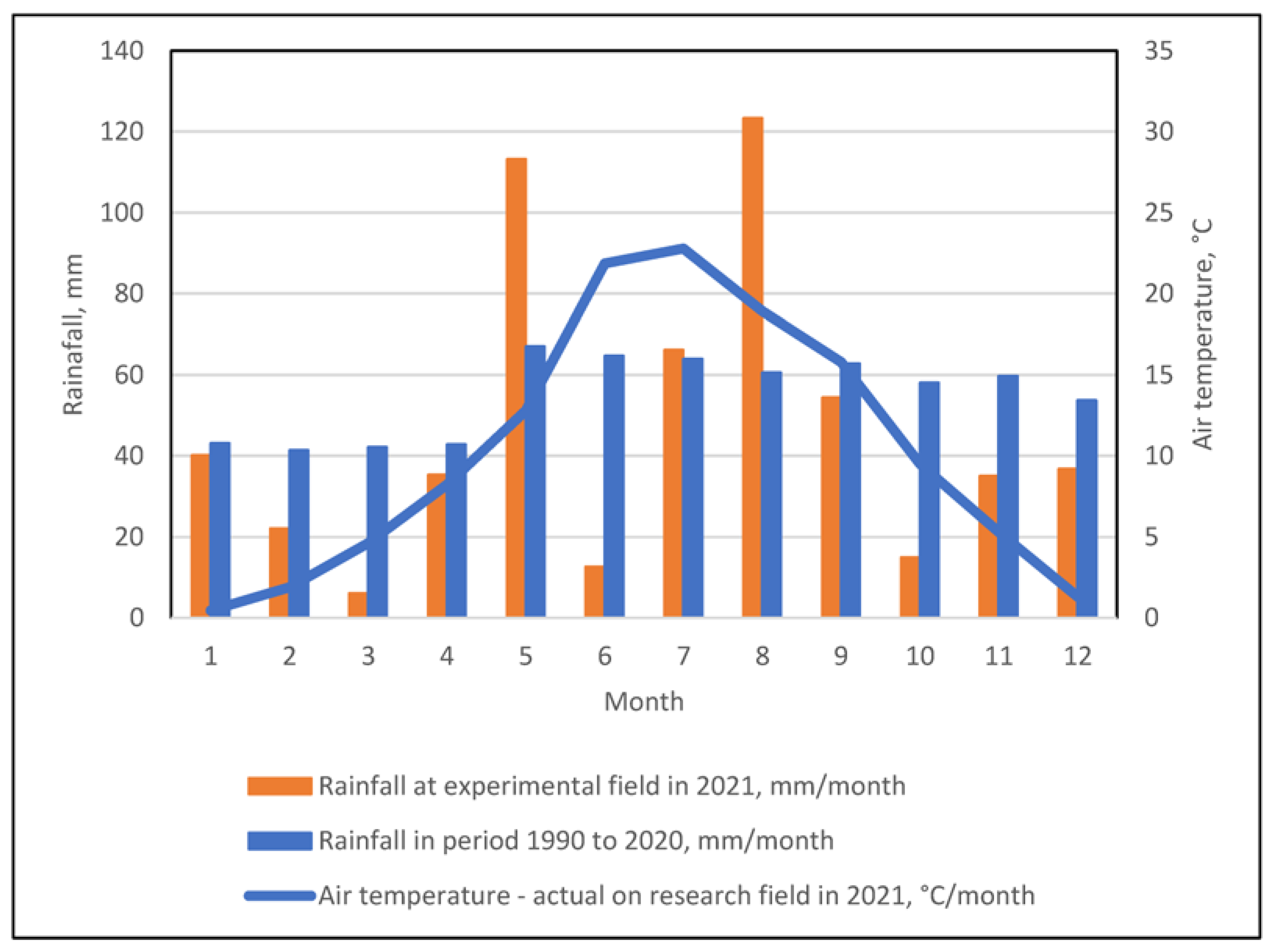
Figure 1. Experimental field showing the direction of the permanent tramlines and the three traffic intensity areas: (A) no traffic area; (B) single pass area; (C) multiple pass/permanent tramline area.
Land 12 00239 g001
Figure 2. Climate parameters of the experimental field, compared to the long-term average values.
Land 12 00239 g002
Figure 3. Rain simulator: a frame having a nozzle and an assembly for sampling water runoff.
Land 12 00239 g003
Figure 4. Slope length of the experimental field (determined from the raw data [33]).
Land 12 00239 g004
Figure 5. Contributing area used for the calculation of the potential soil loss (determined from the raw data [33]).
Land 12 00239 g005
Figure 6. Slope angle in the experimental field (determined from the raw data [33]).
Land 12 00239 g006
Figure 7. Potential yearly soil loss, determined by USLE equation.
Land 12 00239 g007
Figure 8. Potential yearly soil loss, determined by the modified USLE (RUSLE) equation, and targeted points 1 and 2 for in situ measurements.
Land 12 00239 g008
Figure 9. Intensity of water runoff measured in three locations during the simulated rain with the intensity of 1300 mL min−1: (A) no traffic area; (B) single pass area; (C) multiple pass/permanent tramline area.
Land 12 00239 g009
Figure 10. Weight of soil sediments sampled during the simulated rain in the three locations: (A) no traffic; (B) single pass; (C) multiple passes/permanent tramlines.
Land 12 00239 g010
Figure 11. Soil cone penetrometer resistance measured in October 2021 (A—no traffic; B—single pass; C—multiple passes/permanent tramlines) and comparison of differences between the areas (one way ANOVA, α = 0.05; ns = not significant).
Land 12 00239 g011
Table 1. Climate parameters of the study area in 2021, compared to the long-term average values.
ParameterAverage Yearly Value
in the Period 1991–2020, mm [37]
Actual Yearly Value
in Experimental
Field in 2021, mm
Difference,
mm
Relative to Average,
%
otal rainfall, mm660.00560.20−99.8084.88
Air temperature, °C10.7010.29−0.4196.16
Relative air humidity, %71.9075.773.87105.38
Table 2. Estimated soil loss in the experimental field.
CategoryYearly Soil Loss,
t ha−1
USLE [28]USLE [29]
(LS by Wischmeier and Smith, 1978)(LS by Moore and Burch, 1986)
Area, m2Area, %Area, m2Area, %
1<5107,38054.2084,32642.6
25.01–1044,90822.6733,85017.1
310.01–1524,32912.2820,17410.2
415.01–2012,6206.3713,8247.0
520.01–3077573.9216,4478.3
630.01–4010100.5184364.3
740.01–501030.0549332.5
850.01<100.0116,1278.1
Sum:198,117100.00198,117100.0
Table 3. Calculated soil water limits in the monitored locations.
Traffic TreatmentBulk Density, g cm−3Soil Moisture
Content
(Gravimetric), %
Soil Moisture Content
(Volumetric), %
Field Water
Capacity, mm
Point of Decreased
Availability, mm
Wilting Point, mm
A1.5322.8634.89348.9226.8167.7
B1.5522.1434.24342.4222.5164.6
C1.5721.4233.71337.1219.1162.0
Disclaimer/Publisher’s Note: The statements, opinions and data contained in all publications are solely those of the individual author(s) and contributor(s) and not of MDPI and/or the editor(s). MDPI and/or the editor(s) disclaim responsibility for any injury to people or property resulting from any ideas, methods, instructions or products referred to in the content.

