Ecosystem Service Trade-Offs and Spatial Pattern Optimisation under Different Land Use Scenarios: A Case Study in Guanzhong Region, China

Abstract

Understanding the complex interactions (i.e., trade-offs and synergies) among ecosystem services (ESs) and exploring land use optimisation are important to realize regional ecological governance and sustainable development. This study examined Guanzhong Region, Shaanxi Province, as the research object. We established 12 future land use scenarios and projected the future land use patterns under the future climate change scenarios and local development policies. Next, we assessed the four main ecosystem services—carbon sequestration (CS), habitat quality (HQ), soil conservation (SC), and food supply (FS) by using related formulas and the InVEST model. Furthermore, the production possibility frontier (PPF) was used to measure trade-offs and synergistic relationships among ESs, and extract the optimal ES group under the different target needs. The results are as follows: (1) In the future 12 land use scenarios of 2050 in Guanzhong Region, forested land increased evidently in the RCP2.6 ecological protection scenario (18,483.64 km). In the RCP6.0 rapid urban development scenario, construction land showed evident expansion in the central and northeastern areas (4764.52 km²). (2) Compared with the ESs under the future multiple scenarios, CS and HQ achieved the maximum value in the RCP8.5 ecological protection scenario. In the RCP2.6 ecological protection scenario, the amount of SC was the largest (3.81 × 10⁶ t). FS in the RCP2.6 business as usual scenario got the maximum value (18.53 × 10⁶ t). (3) By drawing the optimal PPF curve of multiple scenarios in 2050, trade-off relationships were found between FS and CS, HQ, and SC, and synergistic relationships were found between CS, HQ, and SC. Next, the optimal ES groups under the fitted curve were selected by comparing with the ESs of 2018, and adjusting the land use areas and spatial pattern to finally optimise the relationships between ES and achieve the best land use spatial pattern.

1. Introduction

Ecosystem services (ESs) are defined as “the direct and indirect people obtain from ecosystems” [1], with different types of such services distinguished: provisioning services, supporting services, regulating services, and culture services [2]. With the dramatic expansion of society’s needs, the ability of the natural ecosystem to provide food, fresh water, regulate the climate, and purify water has gradually decreased. Thus, balancing material needs and sustainable ecosystem provision is a big challenge for human society [3,4]. Additionally, ecosystem service is a dynamic process characterised by diversity, complexity, and spatio-temporal heterogeneity [5,6]. Because the supply values of ESs are strongly affected by natural ecological factors and socioeconomic factors, the spatial and temporal differentiation of ESs and their interaction occur [7]. Research on ESs has increasingly focused on exploring the complex interactions between ESs and attempting to optimise trade-off relationships, contributing to the sustainable development of society [8].

The complex relationship between ESs mainly depends on the interdependence of ecosystem function. Moreover, multiple services often interact showing interrelation or nonlinear relations. Research on interactions among ESs has been increasing [9,10,11], and the methods used are mainly statistical methods, spatial mapping, and scenario analysis [12,13,14]. The statistical method analyses the quantitative relationship among ESs [15]. Spatial mapping uses GIS or other tools for spatial analysis, such as spatial overlay and map operation [10]. Scenario analysis is used to construct climate change, ecological protection, and social development scenarios, to analyse the future dynamic changes in the interactions between multiple ESs [11]. The research on the relationship between ESs is mature and standardised, but problems remain. For example, relatively few suitable methods are available for trade-off and synergistic analysis, the spatio-temporal heterogeneity of trade-offs and synergistic relationships requires further research, and the relationships between future services based on scenario analysis have not been identified, and how to balance ESs quantitatively to maximise the ecological benefits remains unclear.

Research has also highlighted the need to consider the impact of land use change on ESs [16]. Constructing land use scenarios has been used to simulate temporal and spatial changes in ecosystem services [17,18]. Researchers have attempted to reveal the potential differences in the trade-offs between ESs [19] and determine which scenarios achieve the optimal ESs value, then the results of further research on these topics might provide a theoretical basis for decision-making regarding regional land use management [20]. Therefore, exploring the relationships between ESs based on land use scenarios facilitates local ecological civilisation construction [21]. However, some research has focused on the relationship between ESs or the influence of land use change on ES solely [22], without exploring the spatial structure optimisation of ESs or how to reasonably allocate land use resources to optimise ESs within a certain area. Therefore, this study focuses on how to select natural or human factors to construct land use scenarios and explore the influence on ESs and offers suggestions for optimising the land use spatial pattern are given.

Guanzhong Region, Shaanxi Province, is the research object. The land use scenarios for 2050 are constructed in combination with global climate change and local government development decisions, the spatial patterns of ESs under different scenarios are simulated, and the impacts of land use change on ESs are analysed based on future climate change and social development policy. Next, the maximum value of ESs in each scenario is extracted to draw the production possibility frontier curve and find the correlation between two ESs. Finally, the best land use pattern is obtained by adjusting recent land use areas and spatial patterns by using the optimal efficiency curve. To explore the balance between ecological protection and socioeconomic development and realise the optimal utilisation of regional resources, this study provides the theoretical and decision-making basis for weighting the increasing demand for ecosystem services and ameliorating ecological environment degradation.

2. Study Area and Data Sources

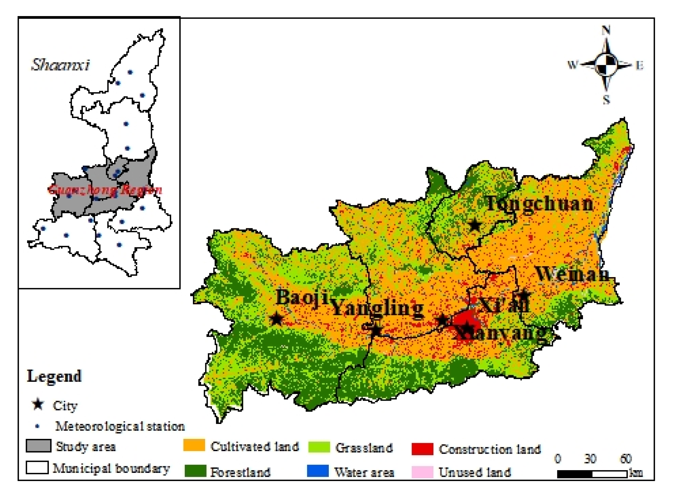
2.1. Study Area

Guanzhong Region is in Central Shaanxi Province, China, and Qinling Mountain traverses east–west in the south, and the Loess Plateau lies to the north. Guanzhong Region includes six city-level administrative divisions: Xi’an, Weinan, Tongchuan, Xiangyang, Baoji Cities, and Yangling. The total area is approximately 55,392.37 km², and the total population is approximately 25.89 million (until 2020). Guanzhong Region has a semi-humid warm temperate continental monsoon climate. The annual average temperature ranges from 12 °C to 14 °C, the average annual precipitation ranges from 550 to 700 mm, and approximately 60% of the annual precipitation falls between June and September [23,24]. Guanzhong Region is an important grain and cotton base and abounds with walnuts, apples, grapes, and other warm temperate fruits. The land use structure is mainly cultivated land (45.17%), followed by forested land and grassland (23.79% and 23.8%, respectively; Figure 1).

Because of implemented strategies, namely, the Western Region Development of China, The Guanzhong Plain Urban Agglomeration (GPUA), “One Belt and One Road,” and other national policies, Guanzhong Region becomes the political, economic, and cultural centre of Western China. Moreover, the GDP showes 62.41% increase from 2010 to 2020. However, because of the rapid economic development, Gaunzhong Region has wasted a substantial amount of its natural resources, and the excessive consumption of ecosystem services has caused irreversible damage. For example, there is a shortage and imbalance of water resources: its total amount accounts for 19% of the entire province, but per capita ownership is 15.4%, and the agricultural irrigation rate accounts for 54%. Regarding energy consumption, coal consumption was 67.46 million tons in 2019, which is 35.5% that of the province and 5.5% more than last year.

Figure 1. Geographical location and land over types of study areas in 2018.

Figure 1. Geographical location and land over types of study areas in 2018.

2.2. Data Sources

The basic data used in this study are as follows: (1) the land use dataset in 2018 was provided by the Resource and Environment Data Cloud Platform (http://www.resdc.cn/), accessed on 23 July 2019; (2) meteorological data, (i.e., average temperature, daily precipitation, maximum daily temperature, minimum daily temperature, sunshine duration, solar radiation) was provided by National Meteorological Information Center of China Meteorological Data Service Center (http://data.cma.cn/en), accessed on 3 September 2019; (3) the soil type map of Guanzhong Region was extracted from a 1:1,000,000 soil dataset of China, and a digital elevation model with a resolution of 30 m was downloaded from Geospatial Data Cloud (http://www.gscloud.cn/), accessed on 29 November 2019; (4) the grain yield and economic statistics of Xi’an City, Tongchuan City, Baoji City, Xianyang City, Weinan City, and 53 counties were from the Statistics Yearbook; and (5) field investigation data and other basic geographic datasets were used. The data sources and preprocessing procedures are listed in Table S1.

3. Methods

3.1. Ecosystem Services Estimation

In this research, considering the regional natural characters and the data availability, methodological capability, etc, we just selected four typical services, such as carbon sequestration, habitat quality as supporting services, soil conservation as regulating services, food supply as provisioning services.

3.1.1. Carbon Sequestration (CS)

CS is the process by which carbon dioxide (CO₂) is emitted and stored safely to replace the direct emission of CO₂ into the atmosphere [25]. By using the photosynthesis equation, the amount of CS can be calculated using the net primary productivity (NPP) to produce every kilogram of organic matter, that is, 1.63 kg of CO₂ can be fixed. The Carnegie Ames Stanford Approach (CASA) model is used to simulate the values of NPP. In the CASA model, two factors are used to represent NPP, the absorbed photosynthetically active radiation (APAR) and the actual solar energy utilisation efficiency (ε) [26]. The equation is as follows:

NPP(x,t) = APAR(x,t) × ε(x,t)

(1)

3.1.2. Habitat Quality (HQ)

HQ refers to the ability of ecosystems to provide sustainable survival and development conditions for individuals’ and populations’ persistence [27]. Generally, habitat quality depends on human activity and land use intensity. The Integrated Valuation of Environment Services and Trade-offs model (InVEST) is widely used to assess habitat quality. Habitat quality and rarity are used as proxies for biodiversity, ultimately estimating the extent of vegetation types across the landscape scale and the state of degradation [28,29]. The formula is as follows:

$$Q_{xj}=H_j\left(1-\left(\frac{D_{xj}^z}{D_{xj}^z+k^2}\right)\right)$$

(2)

where Q_xj represents the quality of habitat quality in parcel x within the LUCC j, D_xj is the total threat level in grid cell x with LULC j, H_j indicates the habitat suitability of LULC type j, z (z = 2.5) and k are scaling parameters, and the k constant is half of maximum D_xj.

3.1.3. Soil Conservation (SC)

Soil erosion directly affects land degradation, agricultural production, ecological degradation, and forest conservation [30,31]. The Revised Universal Soil Loss Equation (RUSLE) is the most empirical model for SC [32]. The RUSLE model is applied to calculate the mean annual SC, which requires land use data, meteorological data, vegetation cover data, soil types and properties, and topographic maps. The RUSLE model is as follows:

A_m = R × K × C × LS × P

(3)

Ap = R × K × C × LS

(4)

A_m = Ap − A_m

(5)

where A_m is the mean annual actual soil erosion (t·ha⁻¹·yr⁻¹), A_p is the potential soil erosion (t·ha⁻¹·yr⁻¹), A_c is the mean annual SC (t·ha⁻¹·yr⁻¹), R is the rainfall erosivity factor (MJ·mm·ha⁻¹·h⁻¹·yr⁻¹), K is the soil erodibility factor (t·h·MJ⁻¹∙mm⁻¹), C is the vegetation cover and management factor, LS includes the slope length factor (L) and the slope steepness factor (S), P is the soil and water conservation measure factor. The C, LS, and P values are dimensionless.

3.1.4. Food Supply (FS)

Provisioning services are the products directly obtained from ecosystems (e.g., food, fresh water, fibre, timber, herb) [33]. The FS is an important provisioning service in the agricultural ecosystem and is a basic material condition for human existence and social development [34]. In this study, land use data and statistical data are used to simulate the FS for each county. The formula is as follows:

G_i = N_i × f_i

(6)

$$f_i=\frac{F_i}{S_i}$$

(7)

where G_i indicates the amount of the ith FS in each grid; N_i is the ith FS area (km²), divided into the unit grid of 1 km × 1 km; f_i represents the yield of the ith food for the unit area (t/km²); F_i indicates total food yield (t·year⁻¹); and S_i represents the total area of the ith food (km²). The source of the FS is obtained from the agricultural yield, containing grain, oil-bearing, vegetable, meat, milk, and aquatic products. Additionally, according to different land use types, grain, oil-bearing, and vegetables belong to the cultivated land, meat and milk belong to the grassland, and aquatic products belong to the water areas.

3.2. Dynamic Changes and Simulation of Land Use Changes

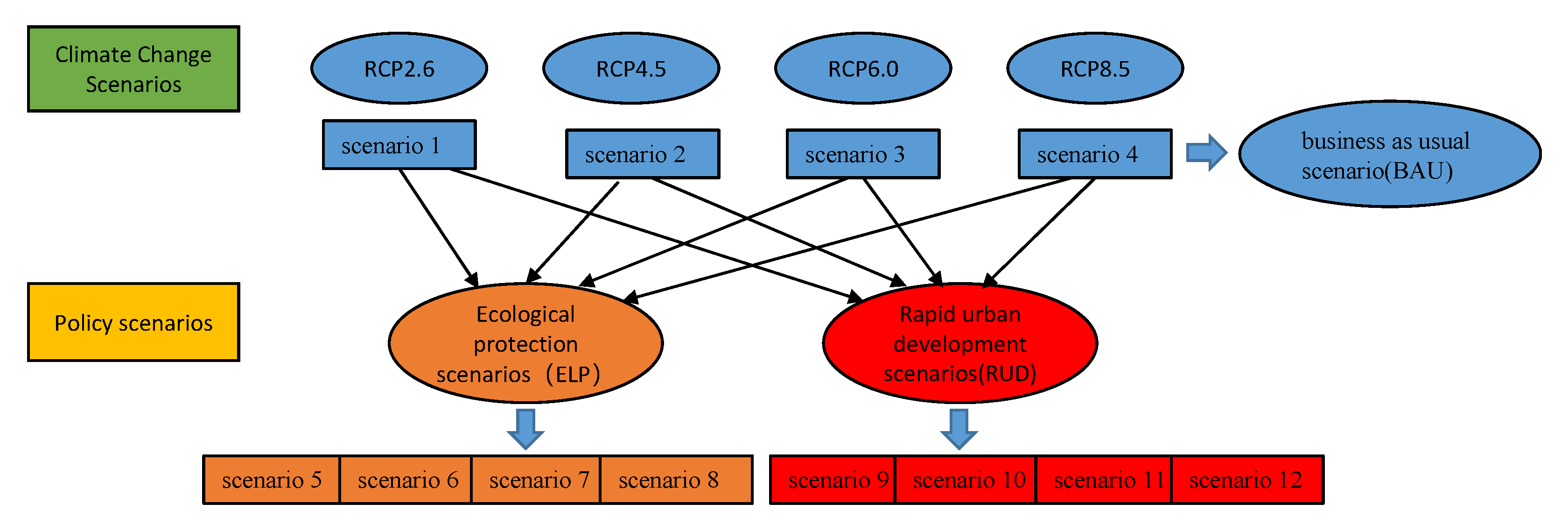
3.2.1. Settings for Land Use Scenarios

Various land use scenarios are established under the global climate change and government policy (e.g., the rapid urban development policy and the ecological protection policy). First, it is based on the four types of atmospheric radiation intensity in the Representative Concentration Pathways (RCPs) proposed in the Fifth Assessment Report of the Intergovernmental Panel on Climate Change (IPCC), and uses the corresponding land use demand scenarios in four scenarios [35]. Next, considering the human influence of land use change, policy scenarios are produced that balance the benefits of ecological protection and economic development.

(1)

Climate change scenarios

The IPCC Fifth Assessment Report (AR5) introduced a new method for developing scenarios. These scenarios span the range of plausible radiative forcing scenarios and are called RCPs. RCPs are characterised by radiative forcing, prescribed pathways for greenhouse gas and aerosol concentrations, and land use change. RCPs scenarios estimate the concentration of greenhouse gases at least 100 years from now and convert it to increased radiation force. Next, four representative climate scenarios are selected: one lower forcing level (RCP2.6), two medium stable scenarios (RCP4.5 and RCP 6.0), and one very high baseline emission scenario (RCP8.5).

(2)

Policy scenarios

The policy scenarios can be regarded as land use policies formulated by the local government, which might balance the interests of regional ecological protection and economic development. Therefore, two policy scenarios are set up. First, according to the policy of grain for green, combined with the characteristics of vegetation slope distribution, the ecological protection scenarios are proposed. Next, considering economic development policies, urban areas are sprawled out, and other factors remain unchanged, and rapid urban development scenarios are formulated. The detailed description is as follows:

① Ecological protection scenarios

Protecting the ecological environment is the primary task. Combined with the policy of returning farmland to forested land and grassland, this scenario reduces cultivated land areas and increases forested land and grassland areas. Thus, high-slope areas are suitable for planting forested land and grassland instead of cultivated land. Combined with the characteristics of the slope distribution of vegetation, the land use types with slopes above 15° will be changed. Therefore, land use conversion from cropland to forestland in the shady slope areas (north, northeast, and northwest) and the eastern slope, the sunny slope (south, southwest, and south), and the western slope would be returned to grassland.

② Rapid urban development scenarios

In the future, urban expansion is projected to accelerate. People will gradually converge in city central areas, resulting in the occupation of marginal land and increases in construction land. Therefore, assumpting that based on the baseline scenario, urban land is gradually expanded to the slower slope areas. That is, land use types with 1 km flat areas (slope less than 5°) adjacent to residential areas are more likely to be transformed into cultivated land.

Based on climate change, ecological protection, and rapid urban development policy, the construction of 12 land use scenarios for 2050 was performed: four climate change scenarios, namely, business-as-usual (BAU) Scenarios 1, 2, 3, 4; four ecological protection (ELP) scenarios, Scenarios 5, 6, 7, 8; and four rapid urban development (RUD) scenarios, Scenarios 9, 10, 11, 12. The detailed parameters of the 12 scenarios are presented in Table S1. The main flowchart is shown in Figure 2.

3.2.2. Land Use Simulation

The Land Change Modeler (LCM) in IDRISI Terrset software was applied to simulate future land use change and mainly contains Multi-Layer Perceptron (MLP), the Markov Chain, and the Soft and Hard Prediction Model. It is used to analyse historical land use to predict future land use change by establishing the spatial variable’s nonlinear relationship [36]. In addition, the major components of the LCM model include land use change analysis, transition modelling, change prediction, and the validation test. The LCM model is easy to operate and provides a better environment for land use change analysis and prediction [37].

We used the land use data under the future climate pattern in IPCC as the baseline scenarios. Next, the future land use in 2050 and the present land use in 2010 were compared and coordinated, the space scale was transformed as 1 km × 1 km, and the land use types were divided into six types (cultivated land, forested land, grassland, water area, construction land, and unused land). Next, the existing land use of 2000 and 2005 was used to predict the land use spatial pattern in 2010, and the predicted land use was compared with the actual land use in 2010. The validation of simulating land use change was provided by the IDRISI model. The standard Kappa coefficient was 0.8814, larger than 0.75, indicating little difference between the results and the actual land use data, and the prediction was relatively reliable. Furthermore, the DEM, slope, distance from settlements, distance from main roads, and distance from major water systems were selected as the drivers, and climate change, ecological protection, and rapid urban development were used as limiting factors.

3.3. Ecosystem Services Relationship Analysis and Spatial Optimisation

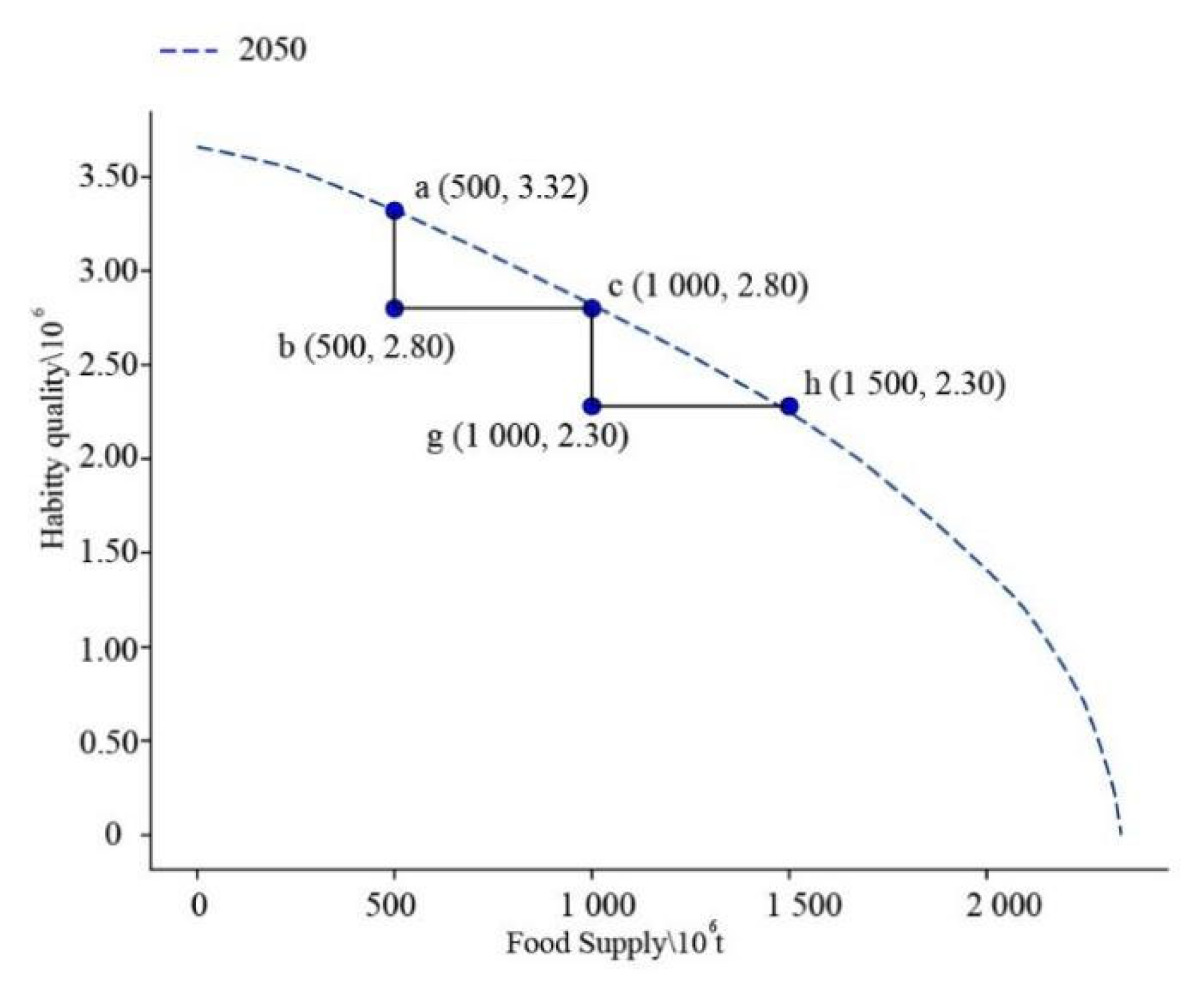
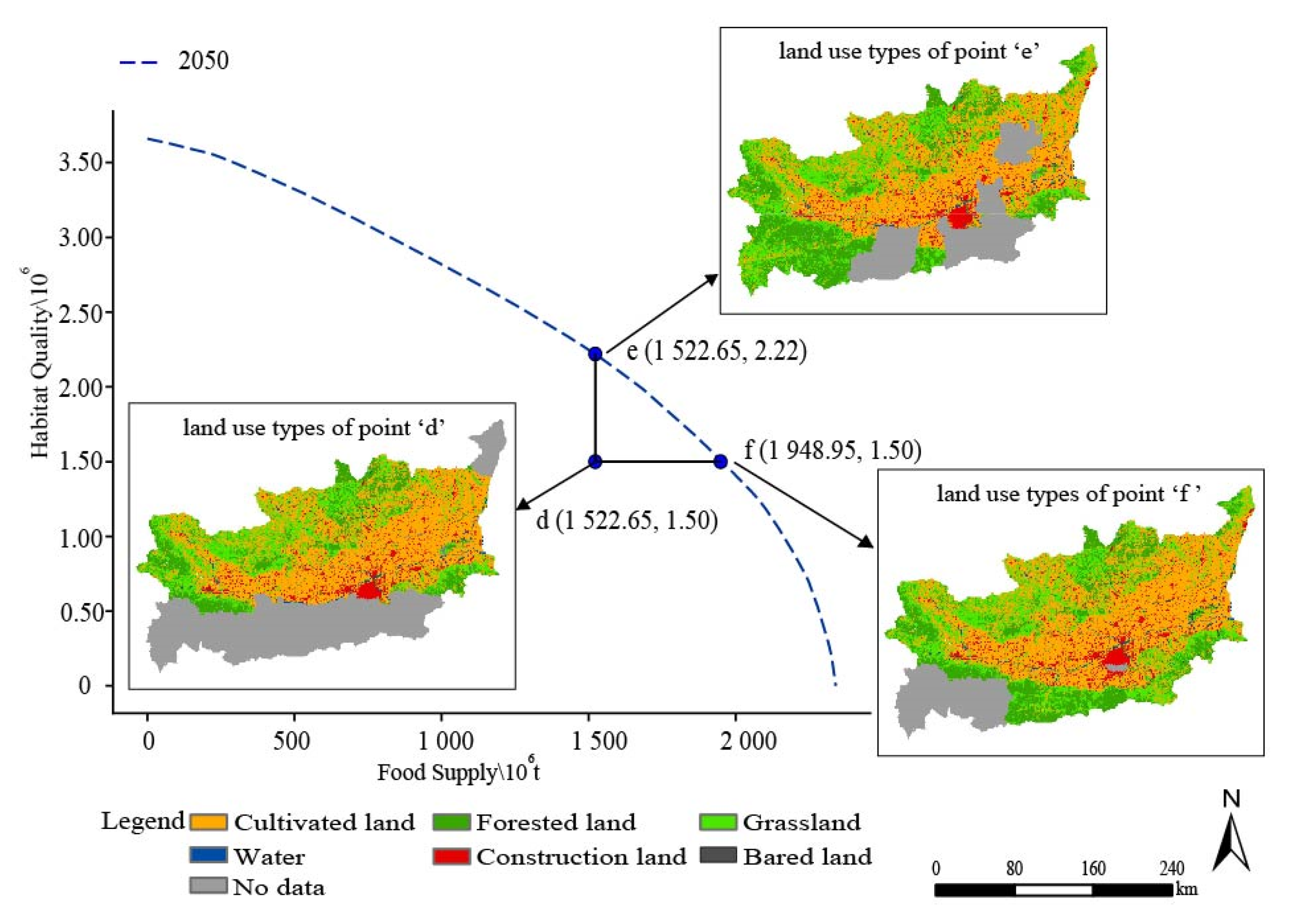
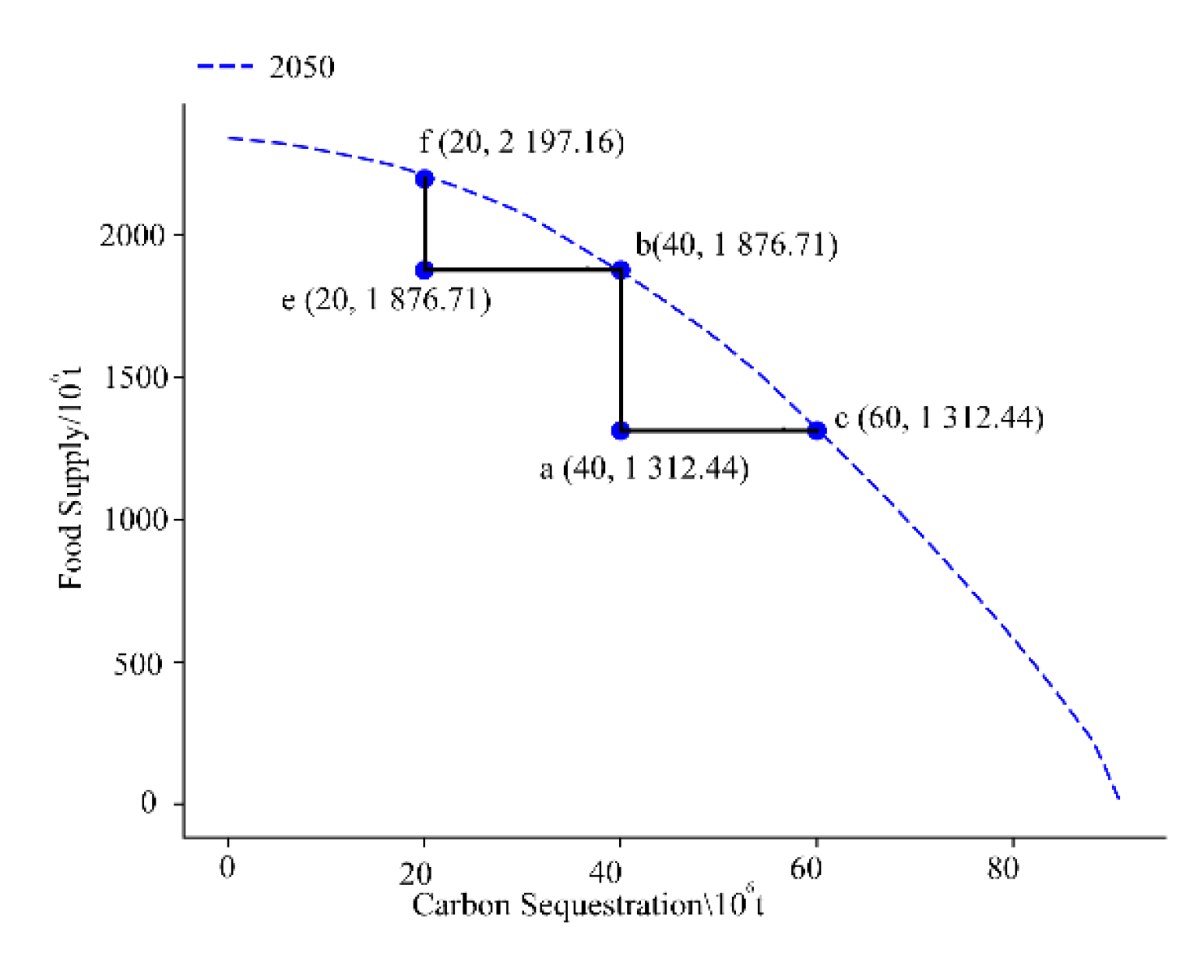
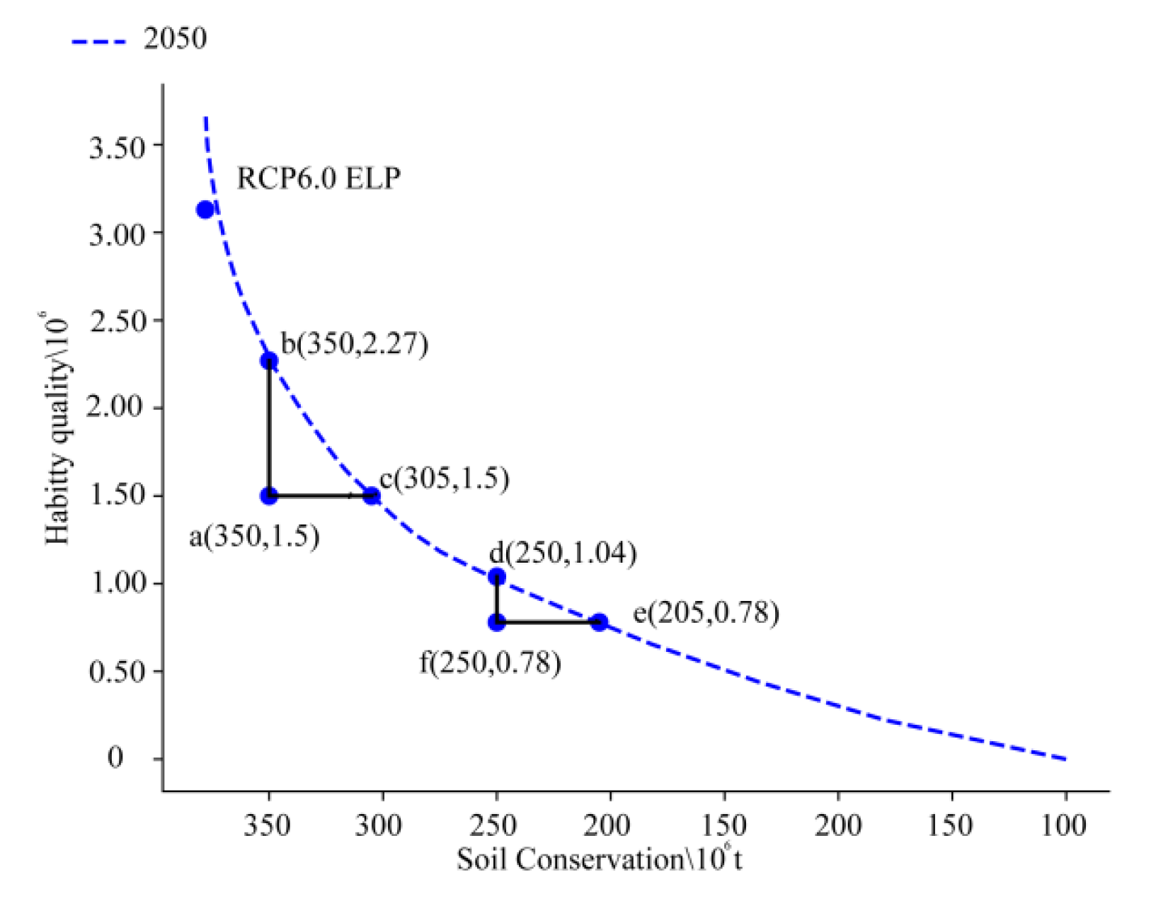
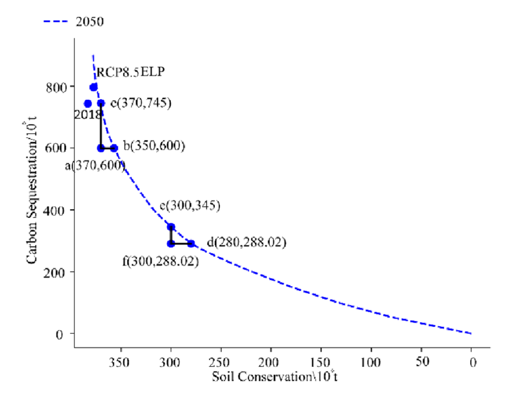
3.3.1. Production Possibility Frontier (PPF)

Ecosystem service optimisation is based on the PPF and is also known as the optimal Pareto efficiency curve. The PPF curve indicates the quantities of one or more products in the given conditions and reflects the potential or excessive problems [38]. In this research, each point on the curve represents the maximum ES values chosen by each scenario. By selecting the optimal ES group on the curve, which means the optimised relationship is exited between two ESs, the optimal land use allocation is achieved. That is, any change in one land use unit will not increase the quantity of one service at the expense of another [39]. The main flowchart is shown in Figure S1.

3.3.2. Measurement of Relationship between ESs

According to the PPF curve, a commonly used method that measures the trade-off and synergy between ESs. We assessed the relationship between ES by comparing the changes in the two services [5]. If the slope of the variation is greater than 0, both represent the same increasing or decreasing trend, and it is synergistic; otherwise, it is a trade-off.

4. Results

4.1. Land Use Changes under Different Future Scenarios in 2050

Combined with future climate change and local development policies, the future land use changes in 2050 were simulated (detailed results are shown in Table S1 and Figure S2). Next, we compared the land use changes under 12 different future scenarios: first, the transverse comparisons that are mainly in climate change scenarios, and next, vertical comparisons that concentrated on the policy development scenarios.

Horizontally, under the same government policy, the four climate change scenarios were compared. We found evident distinctions: Under RCP2.6 climate change scenarios, forested land has the largest increase, followed by cultivated land. For space, forested land shows a significant expansion in the areas of steeper slopes and higher elevation in the southwest of Guanzhong Region, and cultivated land is concentrated in the central areas. In the RCP4.5 climate change scenarios, forested land areas are transformed into cultivated land and grassland and cultivated land accounts for a large proportion. In the RCP6.0 climate change scenarios, the areas of construction land are significantly larger than those in other climate change scenarios. In the RCP8.5 climate change scenarios, grassland areas are relatively larger. This finding showed that much of the cultivated land is converted into grassland and construction land in the central areas, and some forestland is changed to grassland in the northern areas.

Vertically, under the same climate change scenarios, we compared the effects of ecological protection policies and rapid urban development policies. In the ELP scenarios cultivated areas are significantly reduced, and forested land and grassland show a significant increasing trend. In detail, the forested land has the maximum value, accounting for 18,483.64 km² in the RCP2.6 ELP (Scenario 5). The grassland areas have the greatest value, approximately 18,990.81 km² in the RCP8.5 ELP scenario (Scenario 8). The aforementioned results indicate that the policy of returning farmland to forested land and grassland, in which cultivated land with steep slopes is transformed into forested land and grassland, would improve the regional ecological environment level. Compared with the RUD scenarios, the proportion of construction land areas increases significantly. However, the areas of other land use types, such as cultivated land, forested land, grassland, and water areas, show a downward trend. Among them, the maximum area of construction land is in the RCP6.0 RUD scenarios (Scenario 11), which is 4771.88 km². Therefore, the acceleration of urbanisation and population growth result in city areas expanding to the marginal region, and much of the cultivated land, forested land, grassland, and other land use types are occupied by urban land.

4.2. Ecosystem Services Changed under Different Scenarios in 2050

Based on the future land use changes in various scenarios, we simulated the spatial pattern of CS, HQ, SC, and FS in 2050. Because of the lack of temperature, precipitation, sunshine, food yield and other basic data in 2050, we assumed that the changes in ESs are mainly caused by land use changes. So, estimating the ESs in various scenarios, except for the land use changes, the other factors remain unchanged. We took the data of 2018 as the baseline, and the grain yield of 2018 is used in calculating the food supply in 2050. The results of ESs in various scenarios are shown in Table S4 and Figures S3–S6. The results show that changes in ESs under multiple scenarios are closely related to land use changes. For CS, the maximum value of 7.96 × 10⁷ t is in Scenario 8, and the lowest value is in Scenario 11. Thus, the increase in forested land and grassland effectively improves vegetation CS in the ecological protection scenarios. For HQ, the value is larger in the RCP8.5 climate change scenarios but lower in the RCP6.0 climate change scenarios. The maximum value is also obtained in the ELP scenarios, that is, 0.62 in Scenario 8. In the RUD scenarios, the minimum value is 0.57 in Scenario 11. For the amount of SC, the total amount is larger in the RCP2.6 climate change scenarios because the increasing forested land areas can promote soil conservation and water conservation. However, in the RCP8.5 climate change scenarios, construction land areas increase, and some forested land areas are changed into grassland and cultivated land, reducing the capacity of water and soil conservation. For the FS, in the RCP2.6 and RCP4.5 climate change scenarios, the amount of the FS is relatively large because the cultivated land areas are expanded significantly and mainly concentrated in the central areas. The maximum value is 18.53 × 10⁶ t, obtained in Scenario 1. However, when that value is compared with the total amount of 19.89 × 10⁶ t in 2018, a decrease is observed.

For the four climate change scenarios, the most notable results are as follows: in the RCP2.6 climate change scenarios, the values of CS, SC, and FS are much larger. The increase in the proportion of forested land and cultivated land promotes the development of supporting services and regulation services. In the RCP6.0 climate change scenarios, the quantity of CS and HQ is low. In the RCP8.5 climate change scenarios, the amount of FS and SC is low. Almost invariably, the construction land in the two scenarios increases significantly, and the forested land and cultivated land are occupied by urban land. Thus, the abilities of ESs are reduced. On the other hand, the spatial distribution differences of the four ESs are compared in the BAU scenarios, ELP scenarios, and RUD scenarios. The ELP scenarios are conducive to improving the ecological environment and providing supporting services and regulation services. However, because of population growth and urban expansion, the local natural environment has been destroyed, and the value of ESs declined in the RUD scenarios.

4.3. Spatial Pattern Optimisation of Ecosystem Services

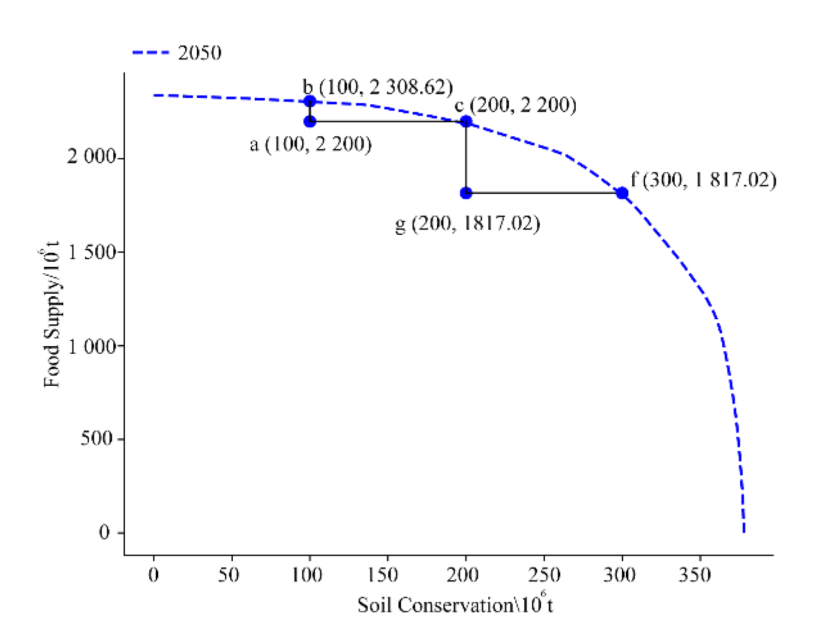
4.3.1. Optimisation of Trade-Off between HQ and FS

There are evident trade-off relationships between HQ and FS, which represents a convex curve (Figure 3). It shows that as FS increases or decreases, HQ decreases or increases, indicating a reverse trend. Details are as follows: The average slope from point “h” to point “c” is k = (2.3 − 2.8)/(1500 − 1000)= −0.5/500, indicating that reducing FS by 500 × 10⁶ t would increase HQ by 0.5 × 10⁶. Moreover, the average slope from point “c” to point “a” is k = (2.8 − 3.32)/(1000 − 500)= −0.52/500, showing that reducing FS with 500 × 10⁶ t will increase HQ to 0.52 × 10⁶.

Figure 4 point “d” (1522.65, 1.50) represents that the amount of FS and HQ is within a certain range of Guanzhong Region. For space, those areas are mainly concentrated in the northern region: cultivated land, 20,682.89 km²; forested land, 5966.30 km²; grassland, 8532.01 km²; water, 353.94 km²; construction land, 2454.43 km²; and unused land, 94.08 km². The land use patterns of point “d” can be optimised by making it fall on the optimal curve. Two extreme methods can be adopted. The first method is to improve the HQ values while not changing the FS values, that is, moving point “d” to point “e” (1522.65, 2.22), which could increase the values of HQ by 0.72 × 10⁶. At this time, the land use pattern of point “d” should be optimised to the land use pattern of point “e”. Specifically, in space, land use areas are expanded to the southwestern region, and some cultivated land areas are removed. The cultivated land areas are 20,422.13 km², forested land areas are 10,342.64 km², grassland areas are 11,006.05 km², water areas are 364.12 km², construction land areas are 2584.02 km², and unused land areas are 84.14 km². The results show that increasing the quality of HQ could decrease the areas of cultivated land and unused land but increase the areas of forested land, grassland, water area, and construction land.

The second method is not changing the amount of HQ and increasing the total amount of FS. Thus, point “d” is moved right to point “f” (1948.98, 1.50) on the curve, and the total amount of FS must be increased by 426.30 × 10⁶ t. Compared with the land use pattern of point “d”, the land use spatial pattern is expanded in the southeastern areas in point “f”, and the construction land is reduced in the central region. The areas of the land use types are as follows: cultivated land, 23,994.27 km²; forested land, 9464.86 km²; grassland, 11,001.91 km²; water, 411.73 km²; construction land, 3002.92 km²; and unused land, 99.09 km². The results show that the areas of cultivated land and grassland increased distinctly by 16.01% and 28.94%, respectively. In conclusion, the PPF curve can be used by changing the land use areas and spatial distribution in combination with the needs of regional ecological and economic development or government policy, and then optimising the spatial pattern of ESs and their relationships quantitatively to achieve the maximum benefits of ESs.

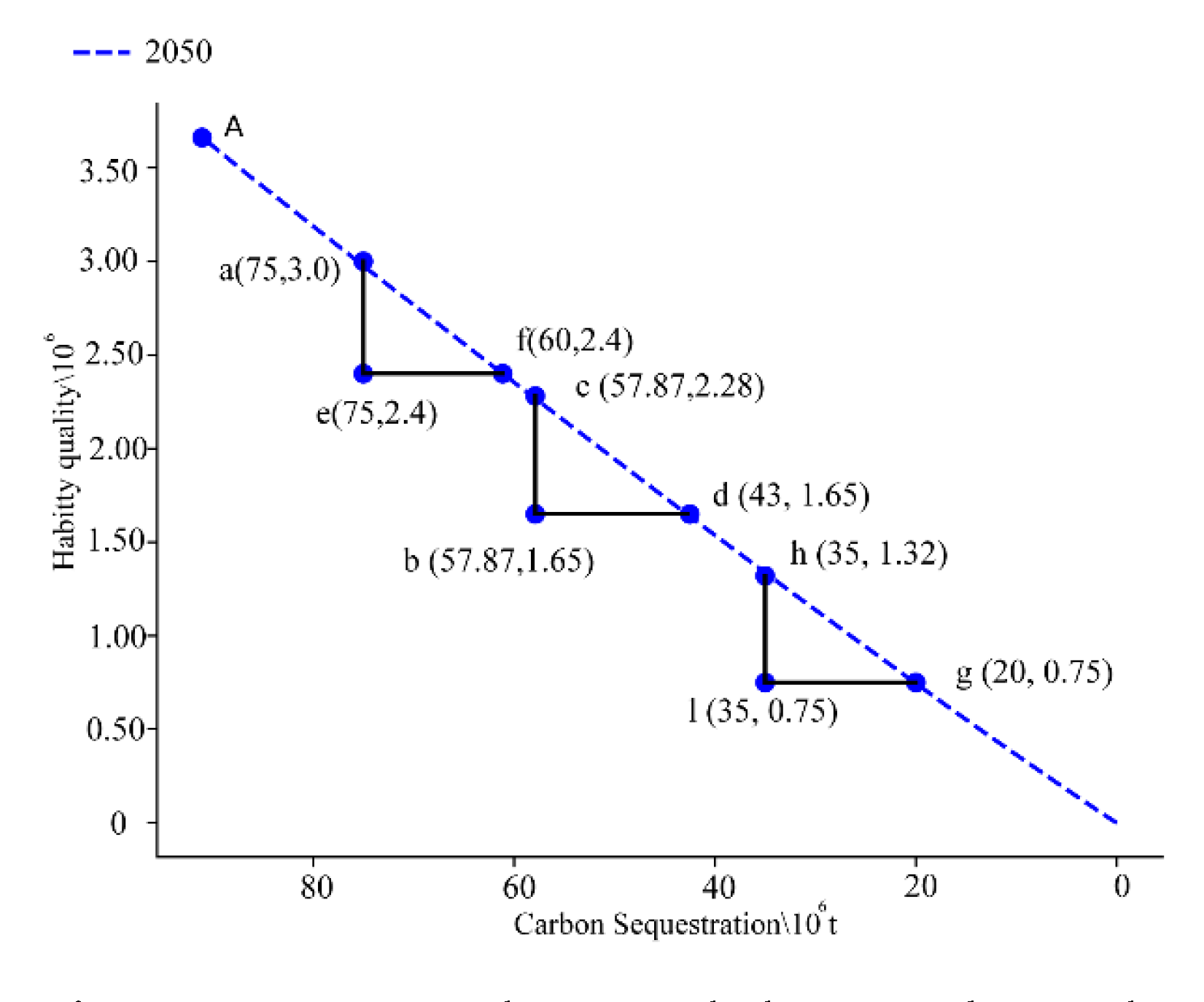
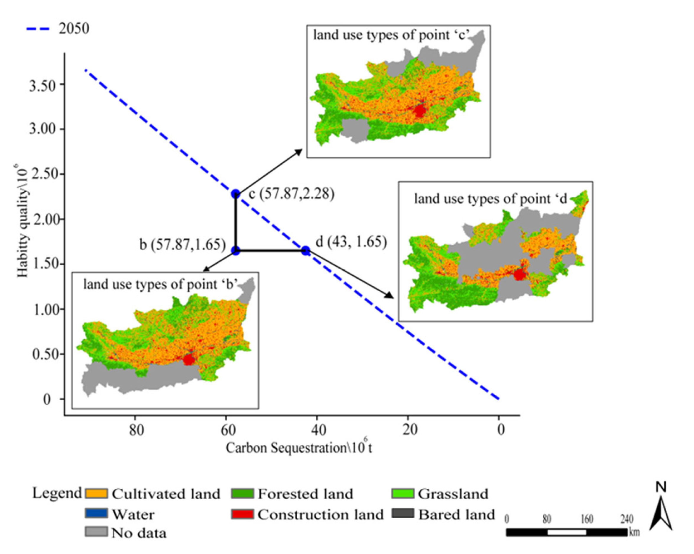
4.3.2. Optimisation of Synergy between HQ and CS

The synergy relationship between HQ and CS indicates a concave curve (Figure 5). As CS increases, HQ increases. On the curve, the average slope from point “g” to point “h” is k = (1.32 − 0.75)/(35 − 20) = 0.57/15, indicating that increasing CS by 15 × 10⁶ t would increase HQ by 0.57 × 10⁶. Additionally, the average slope from point “f” to point “a” is k = (3.0 − 2.4)/(75 − 60) = −0.6/15, showing that increasing CS by 15 × 10⁶ t would increase HQ by 0.6 × 10⁶. From “h”→”c” to “c”→”a”, the average slope will increase. Thus, as CS increases, the value of HQ increases, and both show the same development tendency.

Figure 6 shows that the optimal PPF curve is exited between HQ and CS, representing that the future land use spatial pattern can provide the greatest amount of ESs. It can be seen the values of ESs in 2018 are below the curve, indicating that it exists the potential values. In Figure 6, point “b” is selected as the potential optimisation point to explore the best land use patterns between HQ and CS on the optimal Pareto curve. On the curve, point “b” (57.87, 1.65) represents the amount of CS and HQ within a certain area. The areas are mainly in the north-central and southeastern areas: cultivated land, 21,774.57 km²; forested land, 6725.41 km²; grassland, 9439.48 km²; water, 374.91 km²; construction land, 2696.35 km²; and unused land, 94.08 km². Point “b” can be optimised by two methods. The first method is the total amount of CS remains unchanged, and the values of HQ are increased by moving point “b” to point “c” (57.87, 2.28); HQ is improved by 0.63 × 10⁶. Next, the land use pattern of point “d” can be transferred to point “c”, and the results for the areas are as follows: cultivated land, 20,459.57 km²; forested land, 9286.92 km²; grassland, 10,266.11 km²; water, 381.78 km²; construction land, 2853.91 km²; and unused land, 92.72 km². Therefore, the ESs value of point “b” is optimised to point “c”, and land use patterns would be changed, decreasing cultivated land and unused land but increasing forested land, grassland, water areas, and construction land. Moreover, in the space, it expands to the southwestern and south-central areas.

In the second method, the amount of HQ remains unchanged, and CS is reduced, namely, point “b” moves to the right to point “d” and falls on the optimal PPF, leading to CS decreasing by 14.87 × 10⁶ t. The land use spatial pattern of point “d” shows the areas as follows: cultivated land, 12,410.36 km²; forested land, 9338.86 km²; grassland, 8328.03 km²; water, 272.52 km²; construction land, 1881.53 km², and unused land, 75.13 km². Thus, the land use spatial changes represent that the central and eastern areas are removed, and the southwestern areas are filled. Moreover, the areas of cultivated land, grassland, water, construction land, and unused land decrease as the forested land increases.

Furthermore, the amount of CS and HQ in the Guanzhong Region is optimised. When CS reaches its maximum value in 2018, this phenomenon corresponds to the land use spatial pattern of point “e” (Figure 5). According to the optimal PPF, changing the land use pattern to obtain the optimal ESs combination is possible, that is, point “a” is the best on the optimal Pareto curve. Therefore, point “e” is optimised to point “a”: the method is that CS remains unchanged, HQ is adjusted, and the land use pattern of point “e” should be transferred to point “a”. As shown in Figure 7, the land use types of point “e” in 2018 show the areas as follows: cultivated land, 24,879.51 km²; forested land, 13,280.33 km²; grassland, 13,270.86 km²; water, 612.53 km²; construction land, 3171.22 km²; and unused land, 169.60 km². For land use spatial distribution of point “a” in 2050, the areas are as follows: cultivated land, 17,417.38 km²; forested land, 18,867.97 km²; grassland, 14,672.57 km²; water, 467.99 km²; construction land, 2373.53 km²; and unused land, 15.54 km². For optimising the synergistic relationship between CS and HQ in the whole region, a necessary step is to increase the areas of forested land and grassland and reduce cultivated land, water area, construction land, and unused land, resulting in the total amount of CS remaining unchanged and the values of HQ increasing.

4.3.3. Relationships between Ecosystem Services

As shown in Figure 8, the PPF curve of soil conservation and food supply, and carbon sequestration and food supply, show convex curves, indicating that SC and FS, CS and FS, present trade-off relationships. In the slope of the curve between SC and FS (Figure 8 top), the average slope is from point “f” to point “c” and point “c” to point “b”, that is, k = −382.98/100 and k = −108.62/100, respectively. Using point “d” as an example, the total amount of SC and FS reaches 300 × 10⁶ t and 1400 × 10⁶ t within a certain in 2018. Based on the PPF curve, by increasing FS to point “f” to 1817.02 × 10⁶ t or increasing SC to point “a” reached 343.08 × 10⁶ t. Thus, it depends on different stakeholder needs, and the best land use spatial pattern can be achieved.

Additionally, there is a trade-off relationship between CS and FS (Figure 8 bottom). The average slope indicates that the change rate from point “c” to point “b” and from point “b” to point “f” is −566.27/20 and −320.45/20, respectively. Next, point “a” is selected, which indicates that the total amount of FS and CS is 1312.44 × 10⁶ t and 40 × 10⁶ t, respectively, within a certain range in 2018. Similarly, according to local development objectives, the land use spatial pattern can be optimised by moving point “a” to point “b” or point “c”.

Figure 8. PPF curves between the food supply and soil conservation and carbon sequestration.

Figure 8. PPF curves between the food supply and soil conservation and carbon sequestration.

In addition, there are synergy relationships between SC and HQ. In Figure 9 top, the average slope from point “e” to point “d” and from point “c” is 0.26/45 and 0.77/45, respectively. Moreover, from e→d and c→b, SC increases by 45 × 10⁶ t, and HQ increases by 0.26 × 10⁶ and 0.77 × 10⁶, respectively. Therefore, in the same condition, it could receive more benefits from c→b, indicating that as the amount of SC increases, the increment of HQ will increase. Additionally, the RCP 6.0 ELP scenario is close to the optimal Pareto curve, showing that the relationship between SC and HQ is much better. Furthermore, based on the PPF curve, by changing the land use spatial pattern, point “a” (the amount of SC is 350 × 10⁶ t, HQ is 1.5 × 10⁶) can be optimised to point “b”, by increasing HQ to 2.27 × 10⁶ with the same amount of SC, or to point “c” by reducing SC to 305 × 10⁶ t with the same amount of HQ.

Additionally, it represents a synergy relationship between SC and CS. In Figure 9 bottom, the average slope from point “d” to point “e” and from point “b” to point “c” is 5.70/20 and 14.5/20, respectively, indicating that the cumulative increase in SC is more beneficial to CS. Moreover, the RCP8.5 ELP scenario is close to the optimal Pareto curve, showing that land use pattern is more optimised. The total amount of SC and CS in 2018 of the whole region is below the curve, indicating that the land use resource has great potential. Thus, based on the aforementioned research, SC and CS of point “a” can be optimised to point “c” or point “b” by changing the land use areas or space allocation.

Figure 9. PPF curves between soil conservation and habitat quality and carbon sequestration.

Figure 9. PPF curves between soil conservation and habitat quality and carbon sequestration.

5. Discussion and Conclusions

5.1. Ecosystem Services Trade-Offs and Spatial Optimisation

Understanding the interaction among ESs could promote the reasonable development and utilisation of natural resources from the social ecological system [40]. In this study, we quantitatively analysed the relationships among CS, HQ, SC, and FS using future scenario analysis and PPF. The results show synergistic relationships between CS, HQ, and SC, and the trade-offs between FS and CS, HQ, and SC, which is consistent with the previous research [41]. We also found that on a certain spatial scale, there are evident conflict relationships between provisioning services and regulation services in agricultural ecosystems, and regulation services are the material basis for the sustainable development. For example, the reliable and sufficient supply of fresh water resources is an unavoidable key ecosystem service for the sustainable development of the Guanzhong Region, water conservation play an important part of the local environment protection. Moreover, the growing population lead to the increasing amount of FS, which at the expense of regulation services such as erosion regulation and water purification. Then the trade-offs relationships could occur between the two services. However, considering the regional situation and lack of necessary and sufficient data, and the methodological limitations, we just selected four typical services, but out of cultural services and water conservation service. In the next study, we will break through method limitations, and pick up more indispensable ESs, then explore the complex relationships among multiple services.

Additionally, scenario simulation depends on the current situation to describe the future development trend. Considering uncertainty in the future inevitably affects the simulation accuracy of ESs and increases the uncertainty of trade-off and synergy analysis [42]. This research is based on the global climate change scenario pattern, and the ELP scenarios focus on alleviating the degradation of the ecological environment, and the RUD scenarios enlarge the urban expansion trend. Aiming to assess ecological environment degradation and unreasonable land management, we targeted future scenario analysis and trade-off optimisation to propose reasonable solutions and effective management measures to provide references for regional land use planning, biodiversity protection, and ecological compensation [43]. From the perspective of future scenarios, we explored the relationships between ESs trade-off relationships and land use changes, such as those of cultivated land, forested land, and grassland, respectively, and they play the important role of promoting the increase in FS, SC, and HQ. On the other hand, the increase in construction land could reduce the values of ESs and produce the conflict relationships between ESs. Therefore, human activities, such as afforestation, agricultural activities and urbanisation, could affect the balanced development of ESs [8]. In addition, government decisions comprehensively consider stakeholders’ preferences for different ES benefits or the protection degree, for example, the policy of converting farmland into forested land, nature reserve planning, and ecological compensation mechanism. In further research, establishing many scenarios by comprehensively considering natural or social economic factors would reduce the uncertainty of ES assessment and improve the spatial optimal allocations [44]. Thus, the ESs trade-off relationships should be balanced, and the fragile ecological environment improved to maximise the benefits of regional values of ESs [18,45].

5.2. Limitation and Outlook

This study assessed whether there were trade-offs and synergistic relationships between two services and then explored spatial optimisation by using future various scenarios. Previous studies have mainly used static spatial correlation coefficients to analyse the trade-offs and synergistic relationships among ESs [46]. However, static spatial correlation coefficients ignore the change process of land use patterns and cannot accurately indicate the process and interaction between ESs. Our study used PPF to measure the trade-offs and synergistic relationships and based on the differentiated management policies to establish various land use scenarios, deeply understand the cause of the complex interactions. Notably, this paper analysed the interrelation between two services but did not explore the relationships among multiple services. Moreover, because of the limitation on data sources, the spatial resolution of land use data is 1 km × 1 km, which might cause uncertainty in the spatial interaction between ESs. Future research will further discuss the relationships among multiple services in different spatial–temporal scales and clarify the mechanism of interactions among various ESs. Additionally, there are complicated trade-offs and synergistic relationships among multiple ESs, when the two ESs are optimised and realise the best land use spatial distribution, the third service will be affected. Therefore, to achieve the optimal protection efficiency of ESs and land use spatial optimisation, further research could use multi-objective planning, consider the constraints among various ESs, select priorities based on local development goals, and achieve the optimal pattern.

5.3. Conclusions

Considering future climate change, ecological protection, and government policy factors, this study constructed 12 future land use scenarios in Guanzhong Region. Based on the InVEST model and related equations, future ESs values were simulated under the different land use scenarios. Additionally, with the help of the optimal PPF curves, the maximum values of each ESs were chosen under the various scenarios, and we obtained the optimal ES combinations under the different demands. Finally, the best land use spatial pattern was achieved.

The results showed evident land use spatial pattern changes in different scenarios. Notably, under the RCP2.6 ELP scenario, forested land areas increase significantly, and the southwestern and northern areas with high altitudes and rugged terrain have an evident expansion trend. Under the RCP4.5 BAU scenario, cultivated land areas accounted for more than 38%, and in the RCP6.0 RUD scenario, construction land areas increase evidently and are mainly concentrated in the central and eastern areas. Regarding future ESs, the maximum values of CS and HQ appear in the RCP8.5 ELP scenario because of the better vegetation coverage. Under the RCP4.5 BAU scenario, the amount of SC reaches the maximum value, and in the RCP2.6 BAU scenario FS reaches the maximum value of 18.53 × 10⁶ t. Additionally, the trade-off and synergistic relationships are observed among various ES. We also compare the ESs values of 2018 with the future ES values, the amount of two services within a certain range is below the PPF curve, indicating exist optimisation potential. With the help of the optimal PPF curves, the relationships between ESs can be optimised by adjusting the values of ES, and the best land use spatial structure can be achieved. This study contributes a new idea to measure the trade-offs and synergistic relationships among ESs. This can act as a reference for studies on the optimisation of ES relationships in other regions and provide guidelines for local governments to distribute land use resources rationally.

References

1. Daily, G.C. Nature’s Services: Societal Dependence on Natural Ecosystems; Island Press: Washington, DC, USA, 1997. [Google Scholar]
2. Hassan, R.; Scholes, R.; Ash, N. (Eds.) Ecosystems and Human Well-Being: Current State and Trends; Island Press: Washington, DC, USA, 2005. [Google Scholar]
3. Foley, J.A.; Defries, R.; Asner, G.P.; Barford, C.; Bonan, G.; Carpenter, S.R.; Chapin, F.S.; Coe, M.T.; Daily, G.C.; Gibbs, H.K.; et al. Global consequences of land use. Science 2005, 309, 570–574. [Google Scholar] [CrossRef] [Green Version]
4. Wang, D.; Liang, Y.J.; Peng, S.Z.; Yin, Z.C.; Huang, J.J. Integrated assessment of the supply-demand relationship of ecosystem services in the Loess Plateau during 1992–2015. Ecosyst. Health Sustain. 2022, 8, 2130093. [Google Scholar] [CrossRef]
5. Deng, C.X.; Zhu, D.M.; Nie, X.D.; Liu, C.C.; Li, Z.W.; Liu, J.Y.; Zhang, G.Y.; Xiao, L.H.; Zhang, Y.T. Progress of research regarding the trade-offs of ecosystem services. Chin. J. Eco-Agric. 2020, 28, 1509–1522. (In Chinese) [Google Scholar] [CrossRef]
6. Wang, X.Y.; Peng, J.; Lou, Y.H.; Qiu, S.J.; Dong, J.Q.; Zhang, Z.M.; Vercruysse, K.; Grabowski, R.C.; Meersmans, J. Exploring social-ecological impacts on trade-offs and synergies among ecosystem services. Ecol. Econ. 2022, 197, 107438. [Google Scholar] [CrossRef]
7. Fairbrass, A.; Mace, G.; Ekins, P.; Milligan, B. The natural capital indicator framework (NCIF) for improved national natural capital reporting. Ecosyst. Serv. 2020, 46, 101198. [Google Scholar] [CrossRef]
8. Ran, F.W.; Luo, Z.J.; Wu, J.P.; Qi, S.; Cao, L.P.; Cai, Z.M.; Chen, Y.Y. Spatio temporal patterns of the trade-off and synergy relationship among ecosystem services in Poyang Lake Region, China. Chin. J. Appl. Ecol. 2019, 30, 995–1004. (In Chinese) [Google Scholar] [CrossRef]
9. Makwinja, R.; Kaunda, E.; Mengistou, S.; Alamirew, T. Impact of land use/land cover dynamics on ecosystem service value—A case from Lake Malombe, Southern Malawi. Environ. Monit. Assess. 2021, 193, 492. [Google Scholar] [CrossRef] [PubMed]
10. Fu, Q.; Hou, Y.; Wang, B.; Bi, X.; Li, B.; Zhang, X. Scenario analysis of ecosystem service changes and interactions in a mountain-oasis-desert system: A case study in Altay Prefecture, China. Sci. Rep. 2018, 8, 12939. [Google Scholar] [CrossRef] [Green Version]
11. Peng, K.F.; Jiang, W.G.; Ling, Z.Y.; Hou, P.; Deng, Y.W. Evaluating the potential impacts of land use changes on ecosystem service value under multiple scenarios in support of SDG reporting: A case study of the Wuhan urban agglomeration. J. Clean. Prod. 2021, 307, 127321. [Google Scholar] [CrossRef]
12. Wu, B.Q.; Wang, J.B.; Qi, S.H.; Wang, S.Q.; Li, Y.N. Review of methods to quantify trade-offs among ecosystem services and future model developments. J. Resour. Ecol. 2019, 10, 225–233. [Google Scholar] [CrossRef]
13. Wu, L.L.; Sun, C.G.; Fan, F.L. Multi-criteria framework for identifying the trade-offs and synergies relationship of ecosystem services based on ecosystem services bundles. Ecol. Indic. 2022, 144, 109453. [Google Scholar] [CrossRef]
14. Zhao, T.; Pan, J.H. Ecosystem service trade-offs and spatial non-stationary responses to influencing factors in the Loess hilly-gully region: Lanzhou City, China. Sci. Total Environ. 2022, 846, 157422. [Google Scholar] [CrossRef]
15. Xiao, Y.; Huang, M.; Xie, G.; Zhen, L. Evaluating the impacts of land use change on ecosystem service values under multiple scenarios in the Hunshandake region of China. Sci. Total Environ. 2022, 850, 158067. [Google Scholar] [CrossRef]
16. Bryan, B.A.; Ye, Y.Q.; Zhang, J.; Connor, J.D. Land-use change impacts on ecosystem services value: Incorporating the scarcity effects of supply and demand dynamics. Ecosyst. Serv. 2018, 32, 144–157. [Google Scholar] [CrossRef]
17. Li, C.; Wu, Y.M.; Gao, B.P.; Zheng, K.J.; Wu, Y.; Li, C. Multi-scenario simulation of ecosystem service value for optimization of land use in the Sichuan-Yunnan ecological barrier, China. Ecol. Indic. 2021, 132, 108328. [Google Scholar] [CrossRef]
18. Long, X.; Lin, H.; An, X.; Chen, S.D.; Qi, S.Y.; Zhang, M. Evaluation and analysis of ecosystem service value based on land use/cover change in Dongting Lake wetland. Ecol. Indic. 2022, 136, 108619. [Google Scholar] [CrossRef]
19. Peng, J.; Hu, X.X.; Wang, X.Y.; Meersmans, J.; Liu, Y.X.; Qiu, S.J. Simulating the impact of grain-for-green programme on ecosystem services trade-offs in Northwestern Yunnan, China. Ecosystem. Serv. 2019, 39, 100998. [Google Scholar] [CrossRef]
20. Wang, Y.; Li, X.M.; Zhang, Q.; Li, J.F.; Zhou, X.W. Projections of future land use changes: Multiple scenarios-based impacts analysis on ecosystem services for Wuhan city, China. Ecol. Indic. 2018, 94, 430–445. [Google Scholar] [CrossRef]
21. Bohensky, E.L.; Reyers, B.; Jarrsveld, A.S.V. Conservation in practice: Future ecosystem services in a Southern African River Basin: A scenario planning approach to uncertainty. Conserv. Biol. 2006, 20, 1051–1061. [Google Scholar] [CrossRef]
22. Yang, S.Q.; Zhao, W.W.; Liu, Y.X.; Wang, S.; Wang, J.; Zhai, R.J. Influence of land use change on the ecosystem service trade-offs in the ecological restoration area: Dynamics and scenarios in the Yanhe watershed, China. Sci. Total Environ. 2018, 644, 556–566. [Google Scholar] [CrossRef] [PubMed]
23. Zhang, D.J.; Yang, W.J.; Kang, D.R.; Zhang, H. Spatial-temporal characteristics and policy implication for non-grain production of cultivated land in Guanzhong Region. Land Use Policy 2023, 125, 106466. [Google Scholar] [CrossRef]
24. Shaanxi Local History Office. Shaanxi Yearbook. Xi’an, Shaanxi Province Yearbook Editorial Department. 2021. Available online: http://dfz.shaanxi.gov.cn/sqzlk/sxnj/sxnjwz/nj2021/ (accessed on 5 September 2019).
25. Wang, W.; Li, B.Y.; Ren, Z.Y. Ecosystem service function evaluation: A case study of the yinchuan basin in China. Ecol. Eng. 2017, 106, 333–339. [Google Scholar] [CrossRef]
26. Qin, K.Y.; Li, J.; Liu, J.Y.; Yan, L.W.; Huang, H.J. Setting conservation priorities based on ecosystem services—A case study of the Guanzhong-Tianshui Economic Region. Sci. Total Environ. 2019, 650, 3062–3074. [Google Scholar] [CrossRef] [PubMed]
27. Hall, L.S.; Krausman, P.R.; Morrison, M.L. The habitat concept and a plea for standard terminology. Wildl. Soc. Bull. 1997, 25, 173–182. Available online: https://www.jstor.org/stable/3783301 (accessed on 16 September 2019).
28. Song, Y.; Wang, M.; Sun, X.; Fan, Z.M. Quantitative assessment of the habitat quality dynamics in Yellow River Basin, China. Environ. Monit. Assess. 2021, 193, 614. [Google Scholar] [CrossRef] [PubMed]
29. Sun, X.; Jiang, Z.; Liu, F.; Zhang, D.Z. Monitoring spatio-temporal dynamics of habitat quality in Nansihu Lake basin, eastern China, from 1980 to 2015. Ecol. Indic. 2019, 102, 716–723. [Google Scholar] [CrossRef]
30. Chen, H.; Oguchi, T.; Wu, P. Assessment for soil loss by using a scheme of alterative sub-models based on the RUSLE in a Karst Basin of Southwest China. J. Integr. Agric. 2017, 16, 377–388. [Google Scholar] [CrossRef] [Green Version]
31. Wang, Z.; Wang, J. Changes of soil erosion and possible impacts from ecosystem recovery in the Three-River Headwaters Region, Qinghai, China from 2000 to 2015. J. Resour. Ecol. 2019, 10, 461–471. Available online: http://www.jorae.cn/EN/10.5814/j.issn.1674-764X.2019.05.001 (accessed on 6 September 2019).
32. Zerihun, M.; Mohammedyasin, M.S.; Sewnet, D.; Adem, A.A.; Lakew, M. Assessment of soil erosion using RUSLE, GIS and remote sensing in NW Ethiopia. Geoderma Reg. 2018, 12, 83–90. [Google Scholar] [CrossRef]
33. Costanza, R.; De Groot, R.; Braat, L.; Kubiszewski, L.; Fioramonti, L.; Sutton, P.; Farber, S.; Grasso, M. Twenty years of ecosystem services: How far have we come and how far do we still need to go? Ecosyst. Serv. 2017, 28, 1–16. [Google Scholar] [CrossRef]
34. Sun, Y.J.; Li, J.; Liu, X.F.; Ren, Z.Y.; Zhou, Z.X.; Duan, Y.F. Spatially explicit analysis of trade-offs and synergies among multiple ecosystem services in Shaanxi Valley Basins. Forests 2020, 11, 209. [Google Scholar] [CrossRef] [Green Version]
35. Liu, J.Y.; Li, J.; Qin, K.Q.; Zhou, Z.X.; Yang, X.N.; Li, T. Changes in land-uses and ecosystem services under multi-scenarios simulation. Sci. Total Environ. 2017, 586, 522–526. [Google Scholar] [CrossRef]
36. Gupta, R.; Sharma, L.K. Efficacy of Spatial Land Change Modeler as a forecasting indicator for anthropogenic change dynamics over five decades: A case study of Shoolpaneshwar Wildlife Sanctuary, Gujarat, India. Ecol. Indic. 2020, 112, 106171. [Google Scholar] [CrossRef]
37. Ansari, A.; Golabi, M.H. Prediction of spatial land use changes based on LCM in a GIS environment for Desert Wetlands-A case study: Meighan Wetland, Iran. Int. Soil Water Conserv. Res. 2019, 7, 64–70. [Google Scholar] [CrossRef]
38. Yang, X.N.; Li, J.; Qin, K.Y.; Li, T.; Liu, J.Y. Trade-offs between ecosystem services in Guanzhong-Tianshui economic region. Acta Geogr. Sin. 2015, 70, 1762–1773. [Google Scholar] [CrossRef]
39. Yang, W.; Jin, Y.W.; Sun, L.X.; Sun, T.; Shao, D.D. Determining the intensity of the trade-offs among ecosystem services based on production-possibility frontiers: Model development and a case study. J. Nat. Resour. 2019, 12, 2516–2528. (In Chinese) [Google Scholar] [CrossRef]
40. Zhang, Z.Y.; Liu, Y.F.; Wang, Y.H.; Liu, Y.L.; Zhang, Y.; Zhang, Y. What factors affect the synergy and tradeoff between ES, and how, from a geospatial perspective? J. Clean Prod. 2020, 257, 120454. [Google Scholar] [CrossRef]
41. Li, Z.Z.; Cheng, Q.; Han, H.R. Analyzing Land-Use change scenarios for ecosystem services and their trade-offs in the ecological conservation Area in Beijing, China. Int. J. Environ. Res. Public Health 2020, 17, 8632. [Google Scholar] [CrossRef]
42. Cord, A.F.; Bartkowski, B.; Beckmann, M.; Dittrich, A.; Hermans-Neumann, K.; Kaim, A.; Lienhoop, N.; Locher-Krause, K.; Priess, J.; Schroter-Schlaack, C.; et al. Towards systematic analyses of ecosystem service trade-offs and synergies: Main concepts, methods and the road ahead. Ecosyst. Serv. 2017, 28, 264–272. [Google Scholar] [CrossRef]
43. Hou, Y.; Lü, Y.H.; Chen, W.P.; Fu, B.J. Temporal variation and spatial scale dependency of ecosystem service interactions: A case study on the central Loess Plateau of China. Landsc. Ecol. 2017, 32, 1201–1217. [Google Scholar] [CrossRef]
44. Chen, D.S.; Li, J.; Yang, X.N.; Liu, Y. Trade-offs and optimization among ecosystem services in the Weihe River basin. Acta Ecol. Sin. 2018, 38, 3260–3271. (In Chinese) [Google Scholar] [CrossRef]
45. Dade, M.C.; Mitchell, M.G.E.; McAlpine, C.A.; Rhodes, J.R. Assessing ecosystem service trade-offs and synergies: The need for a more mechanistic approach. Ambio 2018, 48, 1116–1128. [Google Scholar] [CrossRef] [PubMed]
46. Tomscha, S.A.; Gergel, S.E. Ecosystem service trade-offs and synergies misunderstood without landscape history. Ecol. Soc. 2016, 21, 43. [Google Scholar] [CrossRef]
Figure 2. Flowchart of land use scenario setting.
Land 12 00236 g002
Figure 3. PPF curves between habitat quality and food supply.
Land 12 00236 g003
Figure 4. Land use patterns under optimal PPF curves between food supply and habitat quality.
Land 12 00236 g004
Figure 5. PPF curve between habitat quality and carbon sequestration.
Land 12 00236 g005
Figure 6. Land use pattern under optimal PPF curves between habitat quality and carbon sequestration.
Land 12 00236 g006
Figure 7. Land use patterns under optimal PPF curves of Guanzhong Region.
Land 12 00236 g007
Disclaimer/Publisher’s Note: The statements, opinions and data contained in all publications are solely those of the individual author(s) and contributor(s) and not of MDPI and/or the editor(s). MDPI and/or the editor(s) disclaim responsibility for any injury to people or property resulting from any ideas, methods, instructions or products referred to in the content.