
Application of the Optimal Parameter Geographic Detector Model in the Identification of Influencing Factors of Ecological Quality in Guangzhou, China

 ,
,  , ,
, ,
Abstract
:1. Introduction
2. Materials and Methods
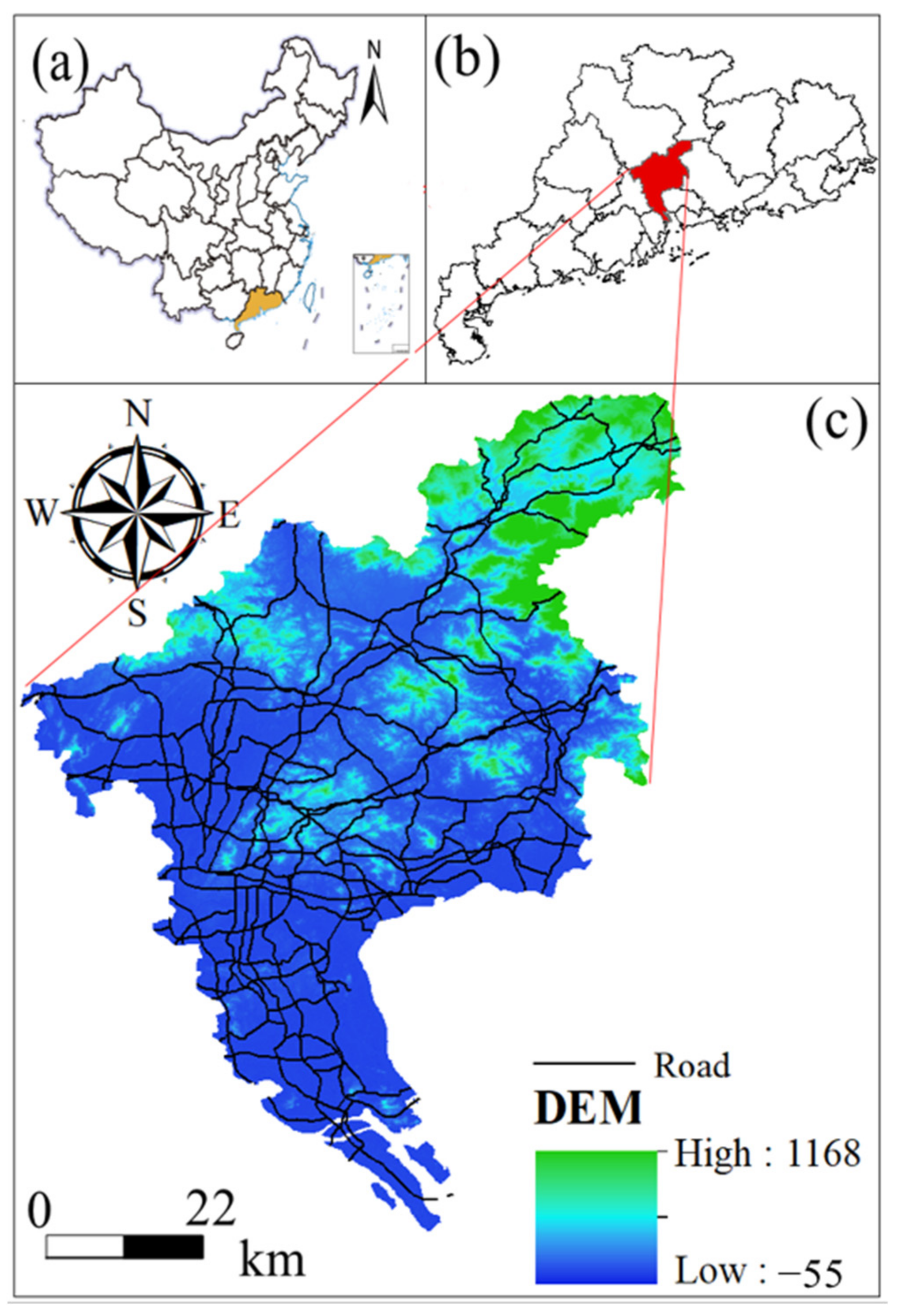
2.1. Study Area
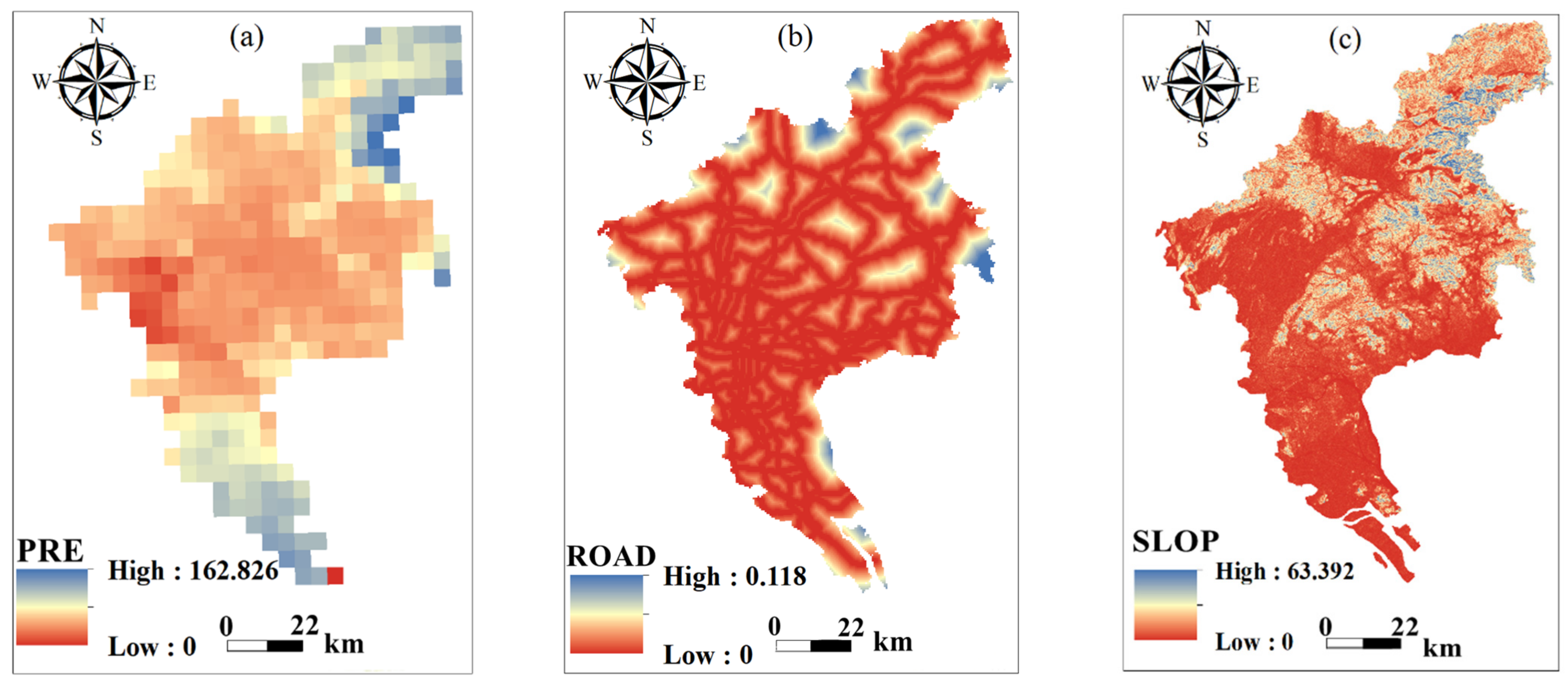
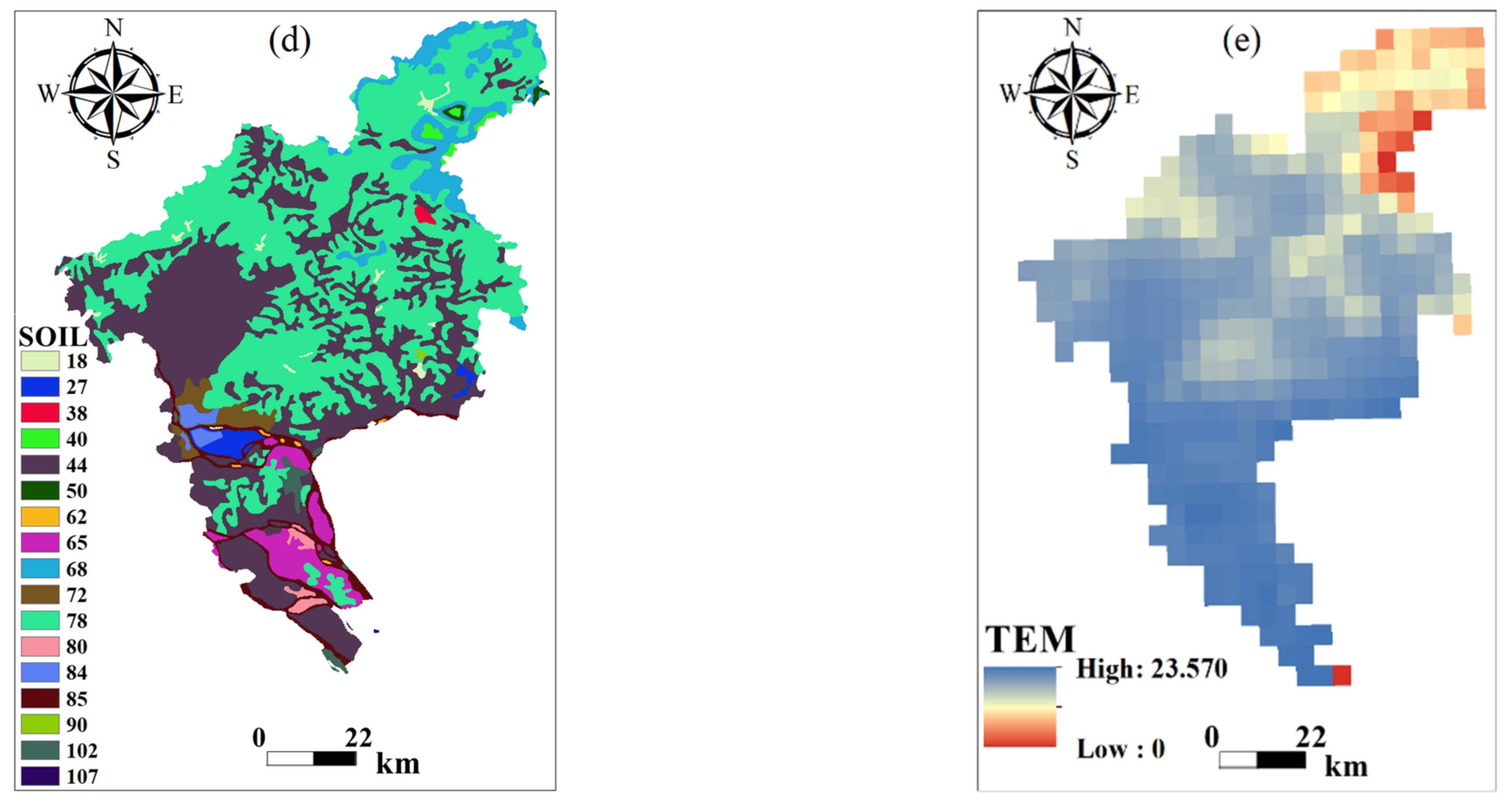
2.2. Data Sources
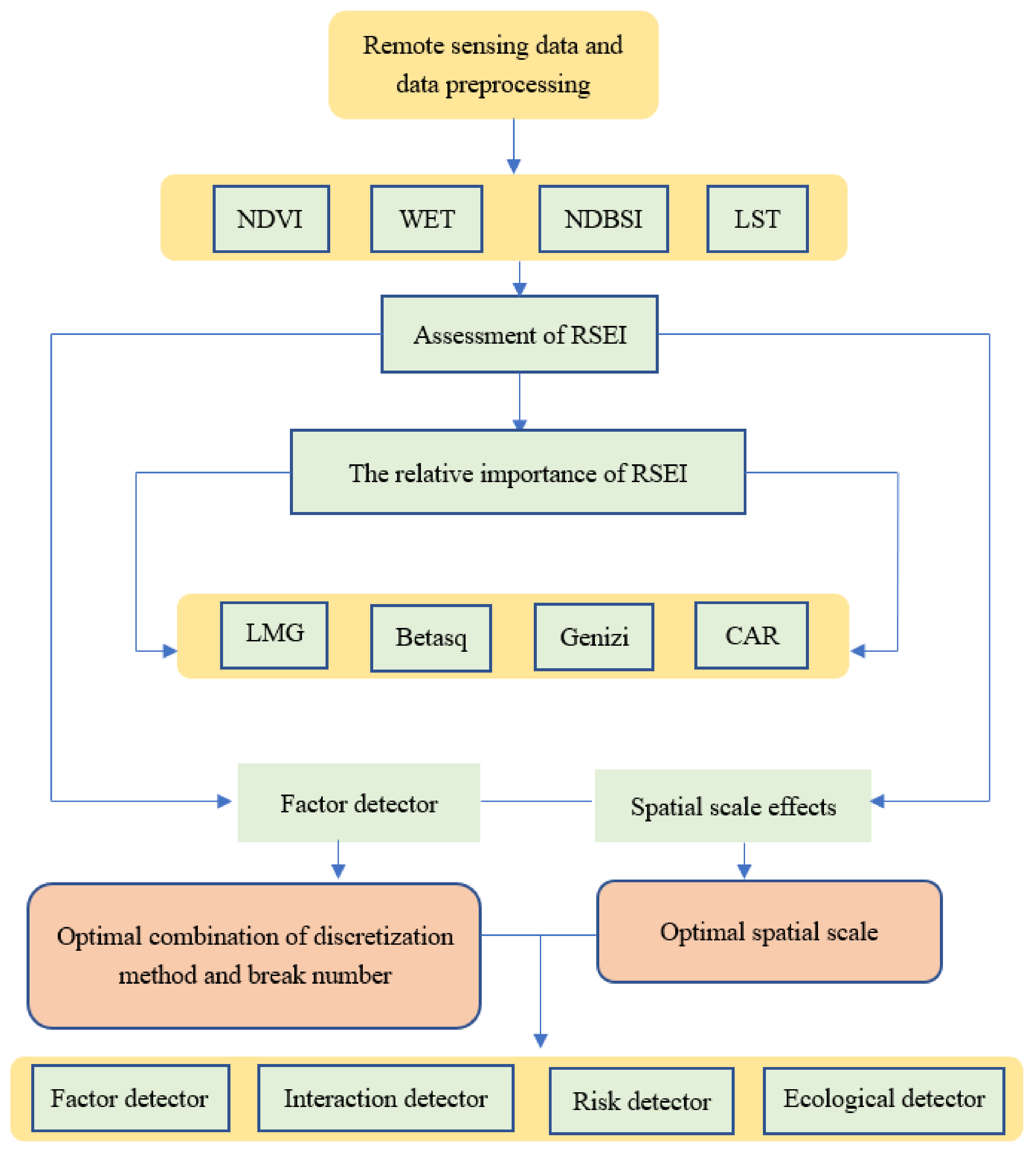
2.3. Research Framework
2.4. Remote Sensing Ecological Index (RSEI)
2.5. Analysis of the Relative Importance of the RSEI
2.6. Optimal Parameter Geographic Detector (OPGD)
2.6.1. Factor Detector
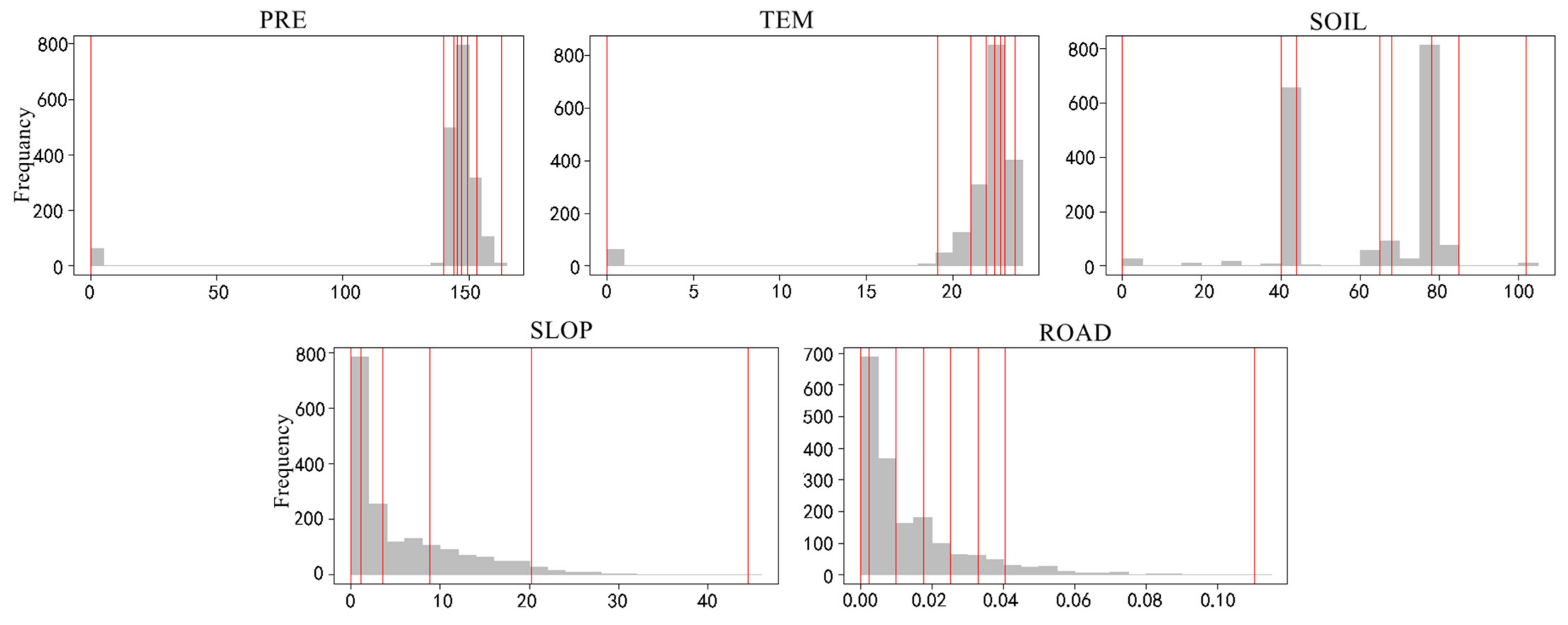
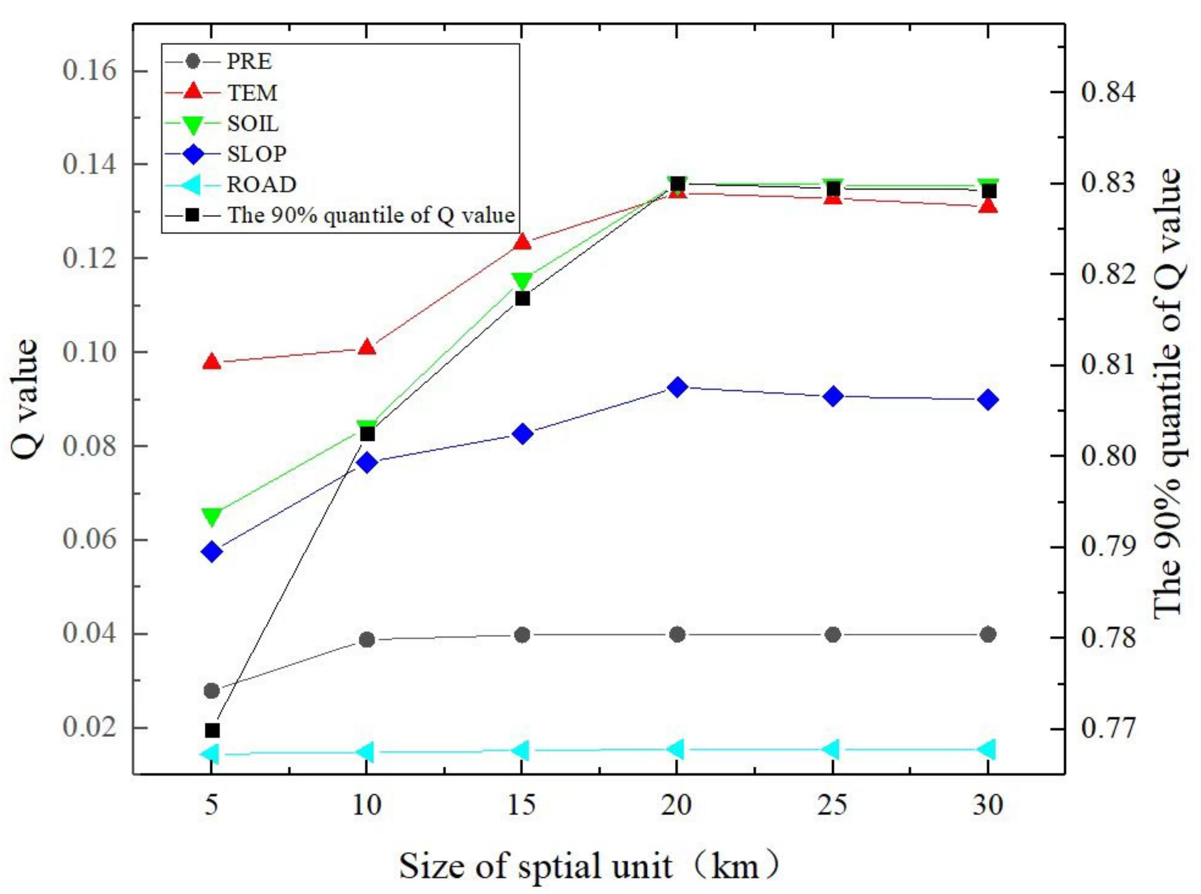
2.6.2. Parameter Optimization
2.6.3. Interaction Detector
2.6.4. Risk Detector
2.6.5. Ecological Detector
3. Results
3.1. Principal Component Analysis of Ecological Indicators
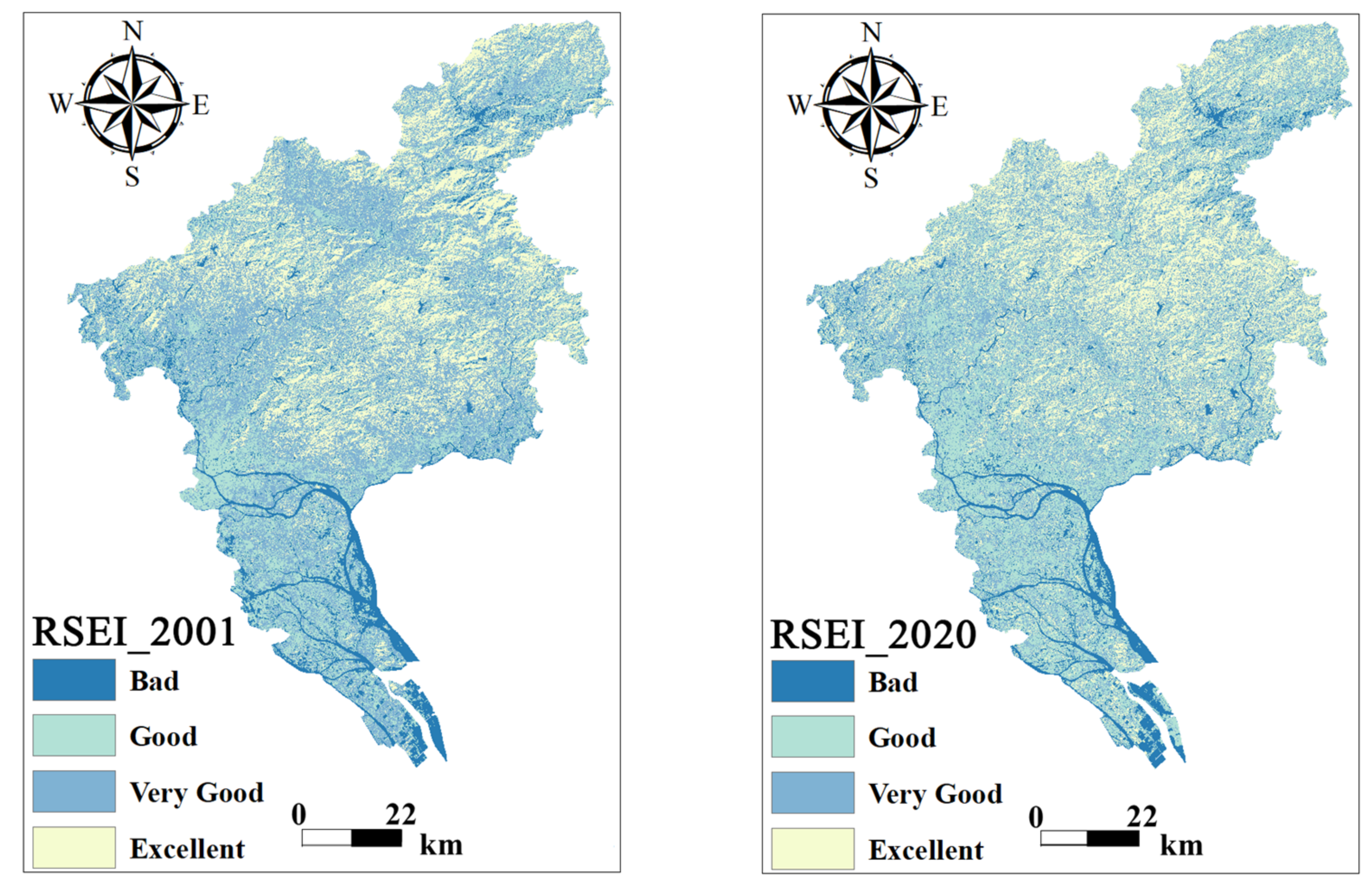
3.2. Temporal and Spatial Changes in Ecological Environment Quality
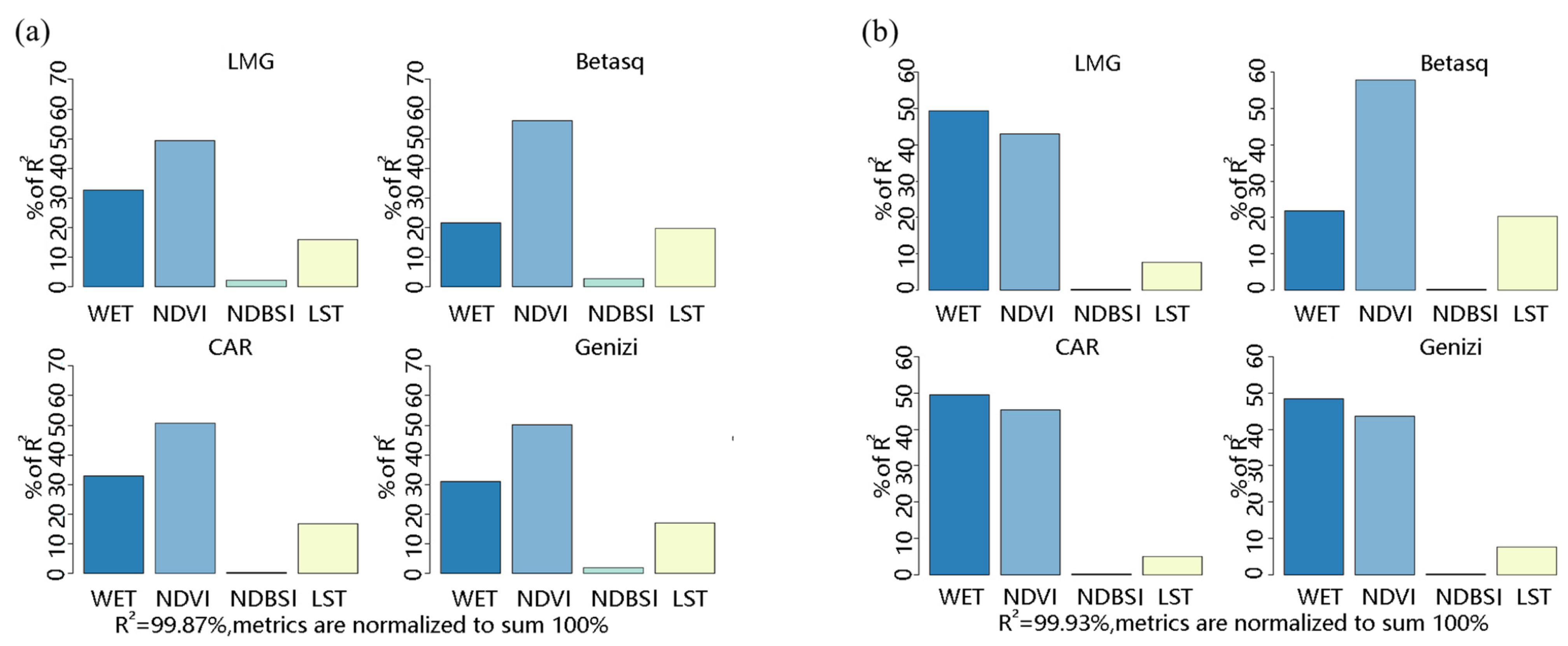
3.3. Analysis of the Relative Importance of the RSEI
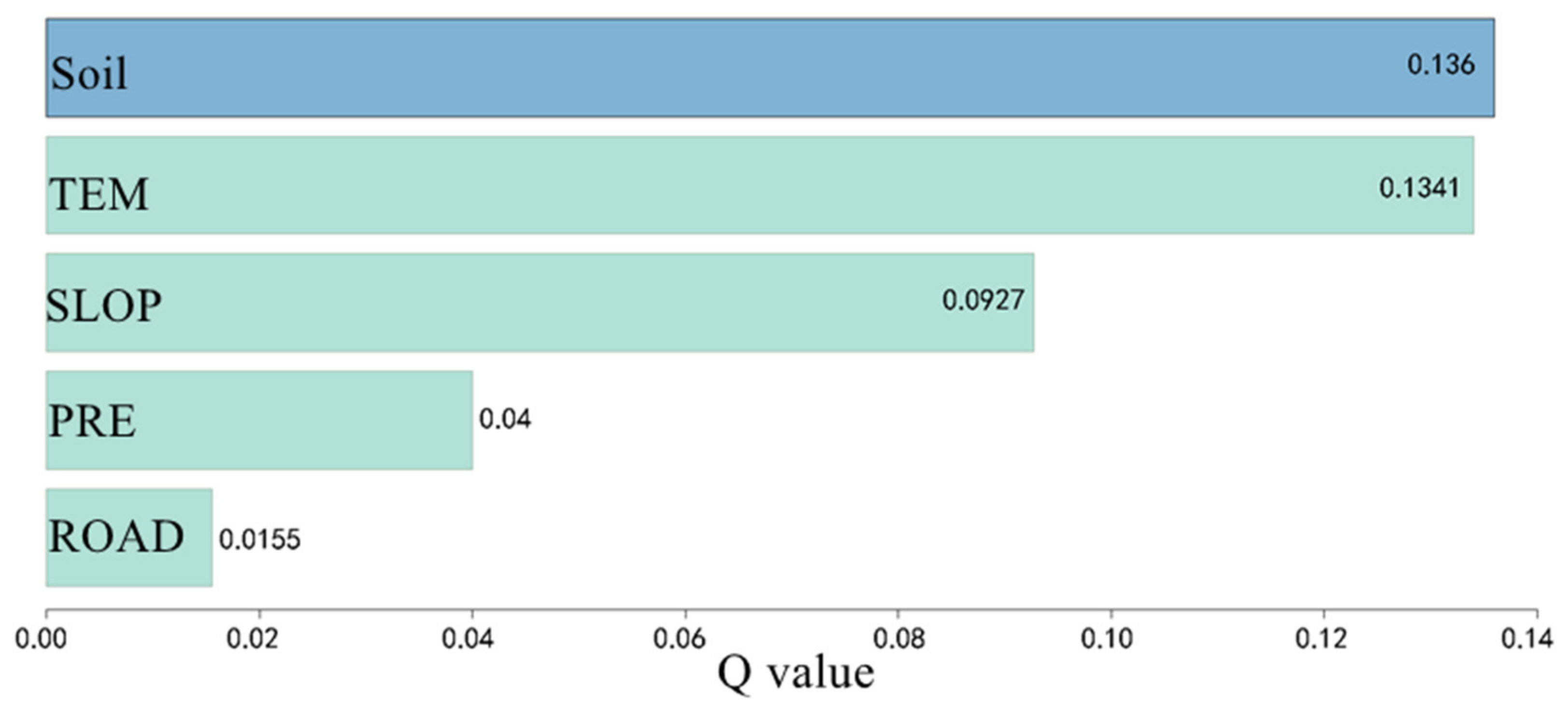
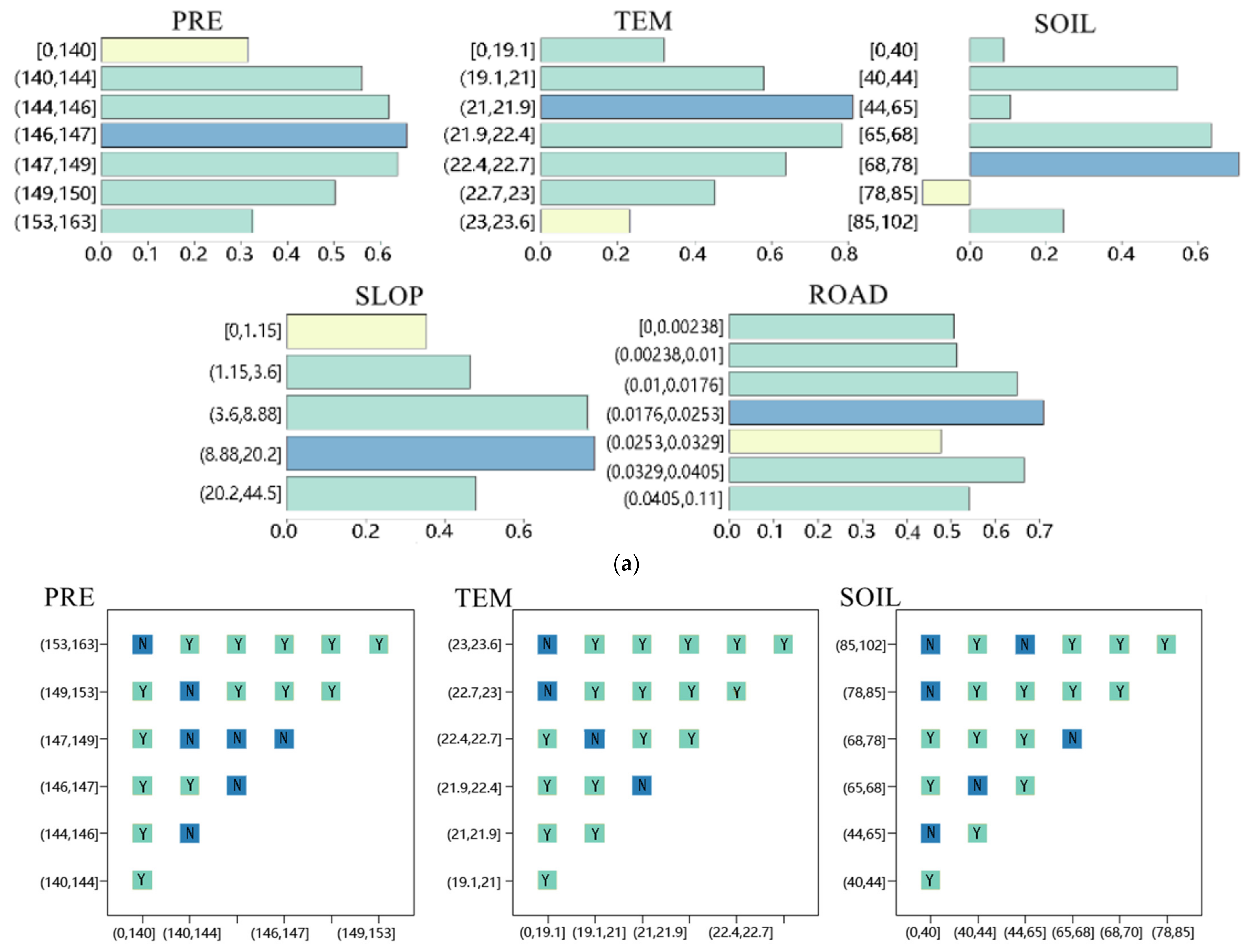
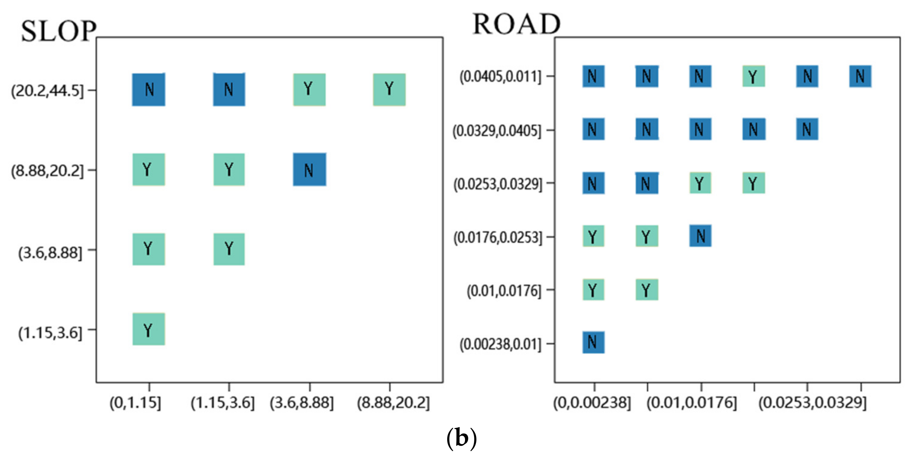
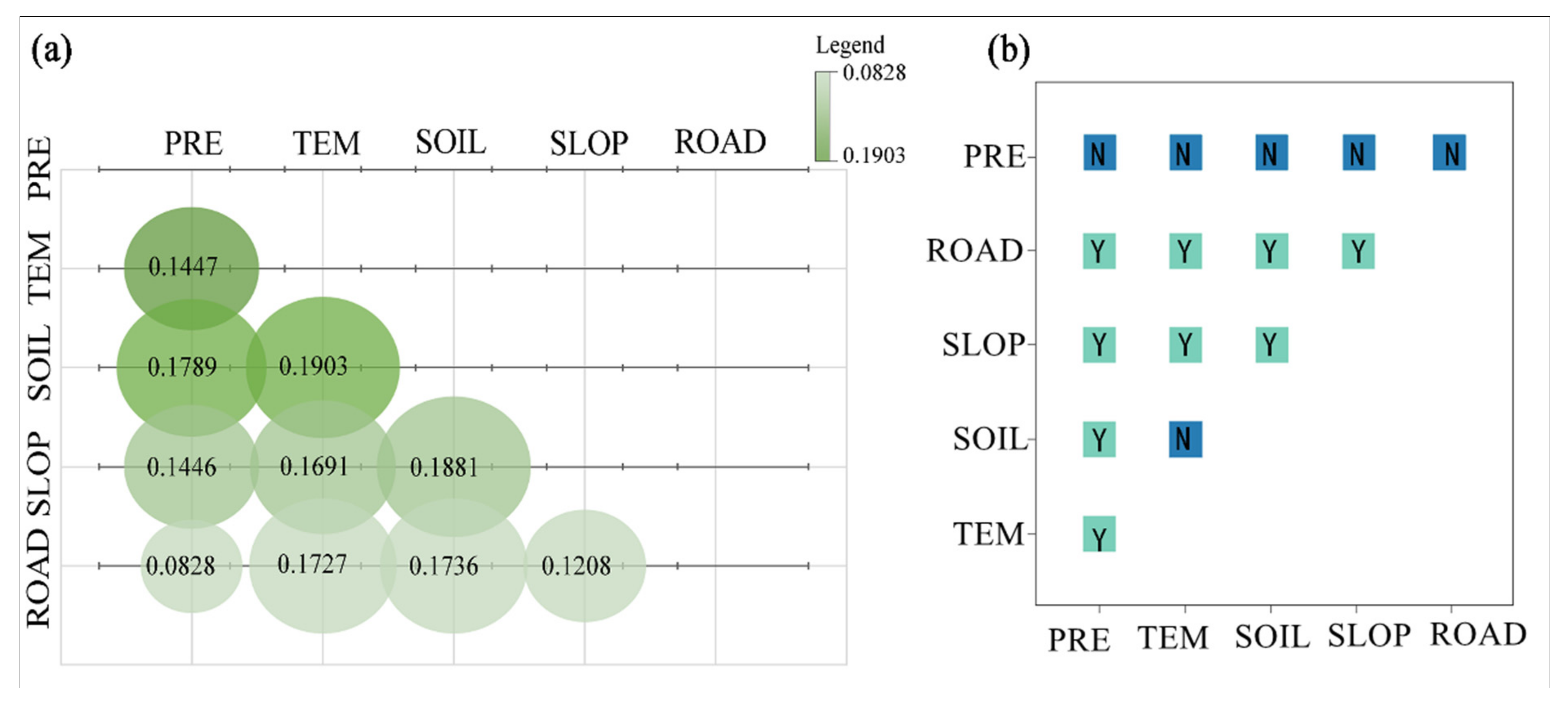
3.4. Analysis of the OPGD
4. Discussions
5. Conclusions
Author Contributions
Funding
Institutional Review Board Statement
Informed Consent Statement
Data Availability Statement
Acknowledgments
Conflicts of Interest
Appendix A
Appendix A.1

| Year | Item | LMG | Betasq | Genizi | CAR |
|---|---|---|---|---|---|
| 2001 | WET | 0.3254 | 0.2161 | 0.3104 | 0.3276 |
| NDVI | 0.4935 | 0.5615 | 0.5008 | 0.5057 | |
| NDBSI | 0.0217 | 0.0260 | 0.0184 | 0.0007 | |
| LST | 0.1594 | 0.1965 | 0.1703 | 0.1660 | |
| 2020 | WET | 0.4936 | 0.2180 | 0.4859 | 0.4953 |
| NDVI | 0.4299 | 0.5785 | 0.4373 | 0.4546 | |
| NDBSI | 0.0007 | 0.0007 | 0.0008 | 0.0007 | |
| LST | 0.0757 | 0.2028 | 0.0761 | 0.0494 |
Appendix A.2
| NO. | Name |
|---|---|
| 18 | Lakes and freshwater |
| 27 | Tide soil |
| 38 | Brown lime |
| 40 | Yellow soil |
| 44 | Rice soil |
| 50 | Yellow–red Soil |
| 62 | Riverine sand |
| 65 | Mizuna rice |
| 68 | Red soil |
| 72 | Grey tide soil |
| 78 | Crimson soil |
| 80 | Submerged rice |
| 84 | Urban area |
| 85 | River |
| 90 | Rice rinsing |
| 102 | Saline rice |
| 107 | Coastal wind and sand |
References
- Hanna, N.; Sun, P.; Sun, Q.; Li, X.; Yang, X.; Ji, X.; Zou, H.; Ottoson, J.; Nilsson, L.E.; Berglund, B.; et al. Presence of Antibiotic Residues in Various Environmental Compartments of Shandong Province in Eastern China: Its Potential for Resistance Development and Ecological and Human Risk. Environ. Int. 2018, 114, 131–142. [Google Scholar] [CrossRef] [PubMed]
- Folke, C.; Biggs, R.; Norström, A.V.; Reyers, B.; Rockström, J. Social-Ecological Resilience and Biosphere-Based Sustainability Science. Ecol. Soc. 2016, 21, 41. [Google Scholar] [CrossRef]
- Olander, L.P.; Johnston, R.J.; Tallis, H.; Kagan, J.; Maguire, L.A.; Polasky, S.; Urban, D.; Boyd, J.; Wainger, L.; Palmer, M. Benefit Relevant Indicators: Ecosystem Services Measures That Link Ecological and Social Outcomes. Ecol. Indic. 2018, 85, 1262–1272. [Google Scholar] [CrossRef]
- Soulsbury, C.D.; White, P.C.L. Human–Wildlife Interactions in Urban Areas: A Review of Conflicts, Benefits and Opportunities. Wildl. Res. 2015, 42, 541. [Google Scholar] [CrossRef]
- Zhang, M.; Zhang, C.; Kafy, A.-A.; Tan, S. Simulating the Relationship between Land Use/Cover Change and Urban Thermal Environment Using Machine Learning Algorithms in Wuhan City, China. Land 2022, 11, 14. [Google Scholar] [CrossRef]
- Lin, Z.; Wu, C.; Hong, W. Visualization Analysis of Ecological Assets/Values Research by Knowledge Mapping. Acta Ecol. Sin. 2015, 35, 142–154. [Google Scholar] [CrossRef]
- Raseduzzaman, M.D.; Jensen, E.S. Does Intercropping Enhance Yield Stability in Arable Crop Production? A Meta-Analysis. Eur. J. Agron. 2017, 91, 25–33. [Google Scholar] [CrossRef]
- Sun, Z.; Sun, W.; Tong, C.; Zeng, C.; Yu, X.; Mou, X. China’s Coastal Wetlands: Conservation History, Implementation Efforts, Existing Issues and Strategies for Future Improvement. Environ. Int. 2015, 79, 25–41. [Google Scholar] [CrossRef]
- Guan, X.; Wei, H.; Lu, S.; Dai, Q.; Su, H. Assessment on the Urbanization Strategy in China: Achievements, Challenges and Reflections. Habitat Int. 2018, 71, 97–109. [Google Scholar] [CrossRef]
- Peng, J.; Pan, Y.; Liu, Y.; Zhao, H.; Wang, Y. Linking Ecological Degradation Risk to Identify Ecological Security Patterns in a Rapidly Urbanizing Landscape. Habitat Int. 2018, 71, 110–124. [Google Scholar] [CrossRef]
- Wang, C.; Yu, C.; Chen, T.; Feng, Z.; Hu, Y.; Wu, K. Can the Establishment of Ecological Security Patterns Improve Ecological Protection? An Example of Nanchang, China. Sci. Total Environ. 2020, 740, 140051. [Google Scholar] [CrossRef] [PubMed]
- Zhang, M.; Chen, W.; Cai, K.; Gao, X.; Zhang, X.; Liu, J.; Wang, Z.; Li, D. Analysis of the Spatial Distribution Characteristics of Urban Resilience and Its Influencing Factors: A Case Study of 56 Cities in China. Int. J. Environ. Res. Public Health 2019, 16, 4442. [Google Scholar] [CrossRef] [PubMed]
- Vörösmarty, C.J.; Rodríguez Osuna, V.; Cak, A.D.; Bhaduri, A.; Bunn, S.E.; Corsi, F.; Gastelumendi, J.; Green, P.; Harrison, I.; Lawford, R.; et al. Ecosystem-Based Water Security and the Sustainable Development Goals (SDGs). Ecohydrol. Hydrobiol. 2018, 18, 317–333. [Google Scholar] [CrossRef]
- Chu, X.; Deng, X.; Jin, G.; Wang, Z.; Li, Z. Ecological Security Assessment Based on Ecological Footprint Approach in Beijing-Tianjin-Hebei Region, China. Phys. Chem. Earth Parts ABC 2017, 101, 43–51. [Google Scholar] [CrossRef]
- Bai, Y.; Jiang, B.; Wang, M.; Li, H.; Alatalo, J.M.; Huang, S. New Ecological Redline Policy (ERP) to Secure Ecosystem Services in China. Land Use Policy 2016, 55, 348–351. [Google Scholar] [CrossRef]
- Asif, M. Growth and Sustainability Trends in the Buildings Sector in the GCC Region with Particular Reference to the KSA and UAE. Renew. Sustain. Energy Rev. 2016, 55, 1267–1273. [Google Scholar] [CrossRef]
- Xu, D.; Yang, F.; Yu, L.; Zhou, Y.; Li, H.; Ma, J.; Huang, J.; Wei, J.; Xu, Y.; Zhang, C.; et al. Quantization of the Coupling Mechanism between Eco-Environmental Quality and Urbanization from Multisource Remote Sensing Data. J. Clean. Prod. 2021, 321, 128948. [Google Scholar] [CrossRef]
- Yue, H.; Liu, Y.; Li, Y.; Lu, Y. Eco-Environmental Quality Assessment in China’s 35 Major Cities Based on Remote Sensing Ecological Index. IEEE Access 2019, 7, 51295–51311. [Google Scholar] [CrossRef]
- Chen, D.; Lu, X.; Hu, W.; Zhang, C.; Lin, Y. How Urban Sprawl Influences Eco-Environmental Quality: Empirical Research in China by Using the Spatial Durbin Model. Ecol. Indic. 2021, 131, 108113. [Google Scholar] [CrossRef]
- Sun, R.; Wu, Z.; Chen, B.; Yang, C.; Qi, D.; Lan, G.; Fraedrich, K. Effects of Land-Use Change on Eco-Environmental Quality in Hainan Island, China. Ecol. Indic. 2020, 109, 105777. [Google Scholar] [CrossRef]
- Cao, H.; Qi, Y.; Chen, J.; Shao, S.; Lin, S. Incentive and Coordination: Ecological Fiscal Transfers’ Effects on Eco-Environmental Quality. Environ. Impact Assess. Rev. 2021, 87, 106518. [Google Scholar] [CrossRef]
- Boori, M.S.; Choudhary, K.; Paringer, R.; Kupriyanov, A. Eco-Environmental Quality Assessment Based on Pressure-State-Response Framework by Remote Sensing and GIS. Remote Sens. Appl. Soc. Environ. 2021, 23, 100530. [Google Scholar] [CrossRef]
- Wu, X.; Zhang, H. Evaluation of Ecological Environmental Quality and Factor Explanatory Power Analysis in Western Chongqing, China. Ecol. Indic. 2021, 132, 108311. [Google Scholar] [CrossRef]
- Lai, J.; Zou, Y.; Zhang, J.; Peres-Neto, P.R. Generalizing Hierarchical and Variation Partitioning in Multiple Regression and Canonical Analyses Using the Rdacca. Hp R Package. Methods Ecol. Evol. 2022, 13, 782–788. [Google Scholar] [CrossRef]
- Song, Y.; Wang, J.; Ge, Y.; Xu, C. An Optimal Parameters-Based Geographical Detector Model Enhances Geographic Characteristics of Explanatory Variables for Spatial Heterogeneity Analysis: Cases with Different Types of Spatial Data. GIScience Remote Sens. 2020, 57, 593–610. [Google Scholar] [CrossRef]
- Yan, Y.; Zhuang, Q.; Zan, C.; Ren, J.; Yang, L.; Wen, Y.; Zeng, S.; Zhang, Q.; Kong, L. Using the Google Earth Engine to Rapidly Monitor Impacts of Geohazards on Ecological Quality in Highly Susceptible Areas. Ecol. Indic. 2021, 132, 108258. [Google Scholar] [CrossRef]
- Roy, D.P.; Kovalskyy, V.; Zhang, H.K.; Vermote, E.F.; Yan, L.; Kumar, S.S.; Egorov, A. Characterization of Landsat-7 to Landsat-8 Reflective Wavelength and Normalized Difference Vegetation Index Continuity. Remote Sens. Environ. 2016, 185, 57–70. [Google Scholar] [CrossRef]
- Zhao, W.; Yan, T.; Ding, X.; Peng, S.; Chen, H.; Fu, Y.; Zhou, Z. Response of Ecological Quality to the Evolution of Land Use Structure in Taiyuan during 2003 to 2018. Alex. Eng. J. 2021, 60, 1777–1785. [Google Scholar] [CrossRef]
- Li, H.; Zhang, A.; Zhao, Y.; Li, J. Remote Sensing Evaluation of Environmental Quality—A Case Study of Cixian County in Handan City. In Proceedings of the International Conference on Geo-Informatics in Sustainable Ecosystem and Society, Guangzhou, China, 21–25 November 2019; Xie, Y., Zhang, A., Liu, H., Feng, L., Eds.; Communications in Computer and Information Science. Springer: Singapore, 2019; Volume 980, pp. 463–474, ISBN 9789811370243. [Google Scholar]
- Guha, S.; Govil, H. Annual Assessment on the Relationship between Land Surface Temperature and Six Remote Sensing Indices Using Landsat Data from 1988 to 2019. Geocarto Int. 2021, 1–20. [Google Scholar] [CrossRef]
- Roy, B.; Bari, E.; Nipa, N.J.; Ani, S.A. Comparison of Temporal Changes in Urban Settlements and Land Surface Temperature in Rangpur and Gazipur Sadar, Bangladesh after the Establishment of City Corporation. Remote Sens. Appl. Soc. Environ. 2021, 23, 100587. [Google Scholar] [CrossRef]
- Xiong, Y.; Xu, W.; Lu, N.; Huang, S.; Wu, C.; Wang, L.; Dai, F.; Kou, W. Assessment of Spatial–Temporal Changes of Ecological Environment Quality Based on RSEI and GEE: A Case Study in Erhai Lake Basin, Yunnan Province, China. Ecol. Indic. 2021, 125, 107518. [Google Scholar] [CrossRef]
- Li, Y.; Wu, L.; Han, Q.; Wang, X.; Zou, T.; Fan, C. Estimation of Remote Sensing Based Ecological Index along the Grand Canal Based on PCA-AHP-TOPSIS Methodology. Ecol. Indic. 2021, 122, 107214. [Google Scholar] [CrossRef]
- Boori, M.S.; Choudhary, K.; Paringer, R.; Kupriyanov, A. Spatiotemporal Ecological Vulnerability Analysis withStatistical Correlation Based on Satellite Remote Sensing in Samara, Russia. J. Environ. Manag. 2021, 285, 112138. [Google Scholar] [CrossRef] [PubMed]
- Ning, L.; Jiayao, W.; Fen, Q. The Improvement of Ecological Environment Index Model RSEI. Arab. J. Geosci. 2020, 13, 403. [Google Scholar] [CrossRef]
- Liu, H.; Jiang, Y.; Misa, R.; Gao, J.; Xia, M.; Preusse, A.; Sroka, A.; Jiang, Y. Ecological Environment Changes of Mining Areas around Nansi Lake with Remote Sensing Monitoring. Environ. Sci. Pollut. Res. 2021, 28, 44152–44164. [Google Scholar] [CrossRef]
- Dang, Y.; He, H.; Zhao, D.; Sunde, M.; Du, H. Quantifying the Relative Importance of Climate Change and Human Activities on Selected Wetland Ecosystems in China. Sustainability 2020, 12, 912. [Google Scholar] [CrossRef]
- Santé, I.; García, A.M.; Miranda, D.; Crecente, R. Cellular Automata Models for the Simulation of Real-World Urban Processes: A Review and Analysis. Landsc. Urban Plan. 2010, 96, 108–122. [Google Scholar] [CrossRef]
- Zhang, M.; Tan, S.; Zhang, Y.; He, J.; Ni, Q. Does land transfer promote the development of new-type urbaniza-tion? New evidence from urban agglomerations in the middle reaches of the Yangtze River. Ecol. Indic. 2022, 136, 108705. [Google Scholar] [CrossRef]
- El Aissaoui, O.; El Alami El Madani, Y.; Oughdir, L.; Dakkak, A.; El Allioui, Y. A Multiple Linear Regression-Based Approach to Predict Student Performance. In Advanced Intelligent Systems for Sustainable Development (AI2SD’2019); Ezziyyani, M., Ed.; Advances in Intelligent Systems and Computing; Springer International Publishing: Cham, Switzerland, 2020; Volume 1102, pp. 9–23. ISBN 978-3-030-36652-0. [Google Scholar]
- Wu, J.; Kobayashi, H.; Stark, S.C.; Meng, R.; Guan, K.; Tran, N.N.; Gao, S.; Yang, W.; Restrepo-Coupe, N.; Miura, T.; et al. Biological Processes Dominate Seasonality of Remotely Sensed Canopy Greenness in an Amazon Evergreen Forest. New Phytol. 2018, 217, 1507–1520. [Google Scholar] [CrossRef]
- Grömping, U. Variable Importance in Regression Models. Wiley Interdiscip. Rev. Comput. Stat. 2015, 7, 137–152. [Google Scholar] [CrossRef]
- Tian, W.; Liu, Y.; Heo, Y.; Yan, D.; Li, Z.; An, J.; Yang, S. Relative Importance of Factors Influencing Building Energy in Urban Environment. Energy 2016, 111, 237–250. [Google Scholar] [CrossRef]
- Luo, Y.; Sun, W.; Yang, K.; Zhao, L. China Urbanization Process Induced Vegetation Degradation and Improvement in Recent 20 Years. Cities 2021, 114, 103207. [Google Scholar] [CrossRef]
- Tan, S.; Zhang, M.; Wang, A.; Ni, Q. Spatio-Temporal Evolution and Driving Factors of Rural Settlements in Low Hilly Region—A Case Study of 17 Cities in Hubei Province, China. Int. J. Environ. Res. Public Health 2021, 18, 2387. [Google Scholar] [CrossRef] [PubMed]
- Zhao, R.; Zhan, L.; Yao, M.; Yang, L. A Geographically Weighted Regression Model Augmented by Geodetector Analysis and Principal Component Analysis for the Spatial Distribution of PM2.5. Sustain. Cities Soc. 2020, 56, 102106. [Google Scholar] [CrossRef]
- Liu, Y.; Zhang, W.; Zhang, Z.; Xu, Q.; Li, W. Risk Factor Detection and Landslide Susceptibility Mapping Using Geo-Detector and Random Forest Models: The 2018 Hokkaido Eastern Iburi Earthquake. Remote Sens. 2021, 13, 1157. [Google Scholar] [CrossRef]
- Wang, W.; Samat, A.; Abuduwaili, J.; Ge, Y. Quantifying the Influences of Land Surface Parameters on LST Variations Based on GeoDetector Model in Syr Darya Basin, Central Asia. J. Arid Environ. 2021, 186, 104415. [Google Scholar] [CrossRef]
- Gu, J.; Liang, L.; Song, H.; Kong, Y.; Ma, R.; Hou, Y.; Zhao, J.; Liu, J.; He, N.; Zhang, Y. A Method for Hand-Foot-Mouth Disease Prediction Using GeoDetector and LSTM Model in Guangxi, China. Sci. Rep. 2019, 9, 17928. [Google Scholar] [CrossRef]
- Sun, D.; Shi, S.; Wen, H.; Xu, J.; Zhou, X.; Wu, J. A Hybrid Optimization Method of Factor Screening Predicated on GeoDetector and Random Forest for Landslide Susceptibility Mapping. Geomorphology 2021, 379, 107623. [Google Scholar] [CrossRef]
- Cook, D.F.; Ragsdale, C.T.; Major, R.L. Combining a Neural Network with a Genetic Algorithm for Process Parameter Optimization. Eng. Appl. Artif. Intell. 2000, 13, 391–396. [Google Scholar] [CrossRef]
- Brest, J.; Maucec, M.S.; Boskovic, B. Single Objective Real-Parameter Optimization: Algorithm JSO. In Proceedings of the 2017 IEEE Congress on Evolutionary Computation (CEC), San Sebastián, Spain, 5–8 June 2017; pp. 1311–1318. [Google Scholar]
- Jayaraman, P.; Whittle, J.; Elkhodary, A.M.; Gomaa, H. Model Composition in Product Lines and Feature Interaction Detection Using Critical Pair Analysis. In Model Driven Engineering Languages and Systems; Engels, G., Opdyke, B., Schmidt, D.C., Weil, F., Eds.; Lecture Notes in Computer Science; Springer Berlin Heidelberg: Berlin/Heidelberg, Germany, 2007; Volume 4735, pp. 151–165. ISBN 978-3-540-75208-0. [Google Scholar]
- Siegmund, N.; Kolesnikov, S.S.; Kastner, C.; Apel, S.; Batory, D.; Rosenmuller, M.; Saake, G. Predicting Performance via Automated Feature-Interaction Detection. In Proceedings of the 2012 34th International Conference on Software Engineering (ICSE), Zurich, Switzerland, 2–9 June 2012; pp. 167–177. [Google Scholar]
- Zhao, Y.; Liu, L.; Kang, S.; Ao, Y.; Han, L.; Ma, C. Quantitative Analysis of Factors Influencing Spatial Distribution of Soil Erosion Based on Geo-Detector Model under Diverse Geomorphological Types. Land 2021, 10, 604. [Google Scholar] [CrossRef]
- Shi, T.; Hu, Z.; Shi, Z.; Guo, L.; Chen, Y.; Li, Q.; Wu, G. Geo-Detection of Factors Controlling Spatial Patterns of Heavy Metals in Urban Topsoil Using Multi-Source Data. Sci. Total Environ. 2018, 643, 451–459. [Google Scholar] [CrossRef] [PubMed]
- Zhu, L.; Meng, J.; Zhu, L. Applying Geodetector to Disentangle the Contributions of Natural and Anthropogenic Factors to NDVI Variations in the Middle Reaches of the Heihe River Basin. Ecol. Indic. 2020, 117, 106545. [Google Scholar] [CrossRef]
- Zha, X.; Gao, X. Ecological Analysis of Kashin-Beck Osteoarthropathy Risk Factors in Tibet’s Qamdo City, China. Sci. Rep. 2019, 9, 2471. [Google Scholar] [CrossRef]
- Xu, H.; Wang, M.; Shi, T.; Guan, H.; Fang, C.; Lin, Z. Prediction of Ecological Effects of Potential Population and Impervious Surface Increases Using a Remote Sensing Based Ecological Index (RSEI). Ecol. Indic. 2018, 93, 730–740. [Google Scholar] [CrossRef]
- Shan, W.; Jin, X.; Ren, J.; Wang, Y.; Xu, Z.; Fan, Y.; Gu, Z.; Hong, C.; Lin, J.; Zhou, Y. Ecological Environment Quality Assessment Based on Remote Sensing Data for Land Consolidation. J. Clean. Prod. 2019, 239, 118126. [Google Scholar] [CrossRef]
- Yuan, B.; Fu, L.; Zou, Y.; Zhang, S.; Chen, X.; Li, F.; Deng, Z.; Xie, Y. Spatiotemporal Change Detection of Ecological Quality and the Associated Affecting Factors in Dongting Lake Basin, Based on RSEI. J. Clean. Prod. 2021, 302, 126995. [Google Scholar] [CrossRef]
- Chen, W.Y. Environmental Externalities of Urban River Pollution and Restoration: A Hedonic Analysis in Guangzhou (China). Landsc. Urban Plan. 2017, 157, 170–179. [Google Scholar] [CrossRef]
- Xie, L.; Xia, B.; Hu, Y.; Shan, M.; Le, Y.; Chan, A.P.C. Public Participation Performance in Public Construction Projects of South China: A Case Study of the Guangzhou Games Venues Construction. Int. J. Proj. Manag. 2017, 35, 1391–1401. [Google Scholar] [CrossRef]
- Yibo, Y.; Ziyuan, C.; Xiaodong, Y.; Simayi, Z.; Shengtian, Y. The Temporal and Spatial Changes of the Ecological Environment Quality of the Urban Agglomeration on the Northern Slope of Tianshan Mountain and the Influencing Factors. Ecol. Indic. 2021, 133, 108380. [Google Scholar] [CrossRef]


| Number | Imaging Data | Satellite/Sensor | Track Number | Cloud Cover (%) |
|---|---|---|---|---|
| 1 | 30 December 2001 | Landsat-5/TM | 122-044 | ≤10 |
| 2 | 28 February 2020 | Landsat-8/OLI_TIRS | 122-044 | ≤10 |
| Year | Indicator | PC1 | PC2 | PC3 | PC4 |
|---|---|---|---|---|---|
| 2001 | NDVI | 0.6488 | 0.1954 | 0.4313 | 0.5957 |
| WET | 0.3282 | 0.7035 | 0.4436 | 0.4478 | |
| NDBSI | −0.6070 | −0.4453 | −0.3223 | −0.5739 | |
| LST | −0.3208 | −0.5182 | −0.7165 | −0.3395 | |
| Eigenvalue | 0.8197 | 0.2769 | 0.1995 | 0.0974 | |
| Percent (%) | 81.2400 | 10.7300 | 6.1500 | 1.8700 | |
| 2020 | NDVI | 0.4837 | 0.2436 | 0.5166 | 0.7065 |
| WET | 0.8748 | 0.1567 | 0.2606 | 0.4083 | |
| NDBSI | −0.0268 | −0.4362 | −0.8156 | −0.5780 | |
| LST | −0.2475 | −0.5321 | −0.2375 | −0.3741 | |
| Percent (%) | 82.5500 | 13.3600 | 3.1700 | 0.9300 | |
| Eigenvalue | 0.6954 | 0.3596 | 0.0417 | 0.0014 |
| Quality Level | 2001 | 2020 | ||
|---|---|---|---|---|
| Area (km2) | Proportion (%) | Area (km2) | Proportion (%) | |
| Bad | 719.2413 | 9.9600 | 660.4146 | 9.1500 |
| Good | 1762.1784 | 24.4000 | 2247.3468 | 31.1200 |
| Very Good | 2961.3069 | 41.0100 | 2334.8574 | 32.3300 |
| Excellent | 1778.8311 | 24.6300 | 1978.9389 | 27.4000 |
Publisher’s Note: MDPI stays neutral with regard to jurisdictional claims in published maps and institutional affiliations. |
© 2022 by the authors. Licensee MDPI, Basel, Switzerland. This article is an open access article distributed under the terms and conditions of the Creative Commons Attribution (CC BY) license (https://creativecommons.org/licenses/by/4.0/).
Share and Cite
Zhang, M.; Kafy, A.-A.; Ren, B.; Zhang, Y.; Tan, S.; Li, J. Application of the Optimal Parameter Geographic Detector Model in the Identification of Influencing Factors of Ecological Quality in Guangzhou, China. Land 2022, 11, 1303. https://doi.org/10.3390/land11081303
Zhang M, Kafy A-A, Ren B, Zhang Y, Tan S, Li J. Application of the Optimal Parameter Geographic Detector Model in the Identification of Influencing Factors of Ecological Quality in Guangzhou, China. Land. 2022; 11(8):1303. https://doi.org/10.3390/land11081303
Chicago/Turabian StyleZhang, Maomao, Abdulla-Al Kafy, Bing Ren, Yanwei Zhang, Shukui Tan, and Jianxing Li. 2022. "Application of the Optimal Parameter Geographic Detector Model in the Identification of Influencing Factors of Ecological Quality in Guangzhou, China" Land 11, no. 8: 1303. https://doi.org/10.3390/land11081303