Article

Analysis Model of the Relationship between Public Spatial Forms in Traditional Villages and Scenic Beauty Preference Based on LiDAR Point Cloud Data

1
College of Landscape Architecture, Nanjing Forestry University, 159 Longpan Rd., Nanjing 210037, China
2
College of Forestry, Nanjing Forestry University, 159 Longpan Rd., Nanjing 210037, China
*
Author to whom correspondence should be addressed.
Land 2022, 11(8), 1133; https://doi.org/10.3390/land11081133
Submission received: 27 June 2022 / Revised: 20 July 2022 / Accepted: 21 July 2022 / Published: 24 July 2022

Abstract

:
Traditional villages are historically, culturally, scientifically and aesthetically valuable, and a beautiful landscape is the primary embodiment of a traditional village environment. Urbanization and modernization have had a great impact on village landscapes. As an important aspect of traditional village landscapes, creating beautiful public spaces is an effective way to attract tourists and improve the well-being of residents. Landscape aesthetic activities are the result of the interaction between landscape objects and aesthetic subjects. Research on the relationship between the form of traditional village public spaces and subjective aesthetic preferences has long been neglected. This research examined 31 public spaces in traditional villages in the Dongshan and Xishan areas in Lake Taihu, Suzhou. An index system of public spatial forms in traditional villages was created, basic data of spatial forms were collected using a hand-held 3D laser scanner, and the value of the spatial forms index was calculated using R language. The scenic beauty estimation (SBE) method was improved, with the estimation of the beauty of the scenic environment based on VR panorama rather than traditional photo media. Parameter screening was performed using correlation analysis and full subset regression analysis, and four models were used to fit the SBE scores and grades. The results show that the majority of public spaces had lower than average SBE scores, and the four key indicators of average contour upper height, solid-space ratio, vegetation cover, and comprehensive closure predicted SBE. In addition, the linear model (R2 = 0.332, RMSE = 64.774) had the most accurate SBE level prediction and the stochastic forest model (R2 = 0.405, RMSE = 63.311) was better at predicting specific SBE scores. The model provides managers, designers, and researchers with a method for the quantitative evaluation of visual landscape preferences and quantitative landscape spatial forms and provides a reference for the protection and renewal of traditional village landscapes.

1. Introduction

Traditional villages are ecologically, historically, culturally, and aesthetically rich. They are places where people can escape the hustle and bustle of urban life, return to nature, and fight off physical and mental fatigue [1,2,3]. Driven by market economics, cultural tourism has developed into one of the main approaches for protecting and developing traditional villages. However, excessive commercial development has had an adverse impact on some traditional village landscapes. Beautiful scenery is a primary tourist attraction that also improves the well-being of village residents [4,5]. Therefore, creating a beautiful scenic environment is an important part of landscape planning and design in traditional villages. Scenic beauty is the subjective impression of features in the landscape and is the product of the interaction between the physical features of the landscape and the individuals observing those features [6,7]. Therefore, both subjective and objective factors affect aesthetic perception. Subjective factors include emotional experience, psychological needs, historical and cultural significance, and spiritual value [8,9,10,11], while objective factors include the physical form, texture, features, and colors of the environment [12,13,14,15]. This paper explores the relationship between objective spatial forms and subjective aesthetic preference in public spaces in traditional villages in Dongshan and Xishan on Lake Taihu.
At present, much research on public space focuses on the urban perspective, emphasizing “collectivity” and “visibility”, which can be understood as gathering places that promote and facilitate social interaction. There is no clear definition of public space in traditional villages, and relevant urban public space theories are used for reference. In this research, public space refers to outdoor open spaces composed of vertical interfaces, top interfaces and bottom interfaces built of natural and artificial materials. It includes such spaces as squares, plazas, parks, and pedestrian-friendly streets. These are spaces where villagers and tourists gather to engage in daily activities, communicate, and relax. “Space” is created by the interrelation between physical space and the individual who perceives it. Landscape aesthetic preference refers to an individual’s or group’s differentiated decision-making. It uses experience, psychological needs, and mental state to evaluate landscapes that reflect the subject’s aesthetic preferences for the scenic environment [6,16,17]. Existing research points to a significant correlation between spatial physical form and landscape aesthetic preference [18,19,20]. The key to exploring the relationship between these is developing effective scientific depictions of the physical variables that represent spatial forms and scientifically measure the landscape aesthetic preferences [15,21,22].

2. Related Works

Most existing studies are based on image data from Worldview, Quick Bird and Landsat [23,24,25], through RS, GIS, Fragstats, and other technical platforms [26,27,28]. Moran’s index of spatial correlation, landscape pattern index, morphological spatial analysis (MSPA), and gradient analysis are used for the quantitative study of landscape spatial forms at regional, urban, and city block or neighborhood levels [29,30,31,32]. This type of method can be used to rapidly obtain the top information data of the space, but the data below the top occluder are often not collected, or the accuracy is insufficient, and the data are distorted. Therefore, this approach is not suitable for the quantitative study of spatial forms at the micro-scale in rural landscapes. Quantitative research on small-scale spatial forms mainly relies on traditional surveying and mapping, using tools such as tape measures, perimeter and digital cameras to stay in two-dimensional paper space. The accuracy of these methods is low. Quantification of forms of public space in traditional villages, unlike in urban spaces, lacks accurate three-dimensional data sources. Compared to the generally more regular façades of urban architectural spaces, traditional manual measurement of smaller-scale village open space is less effective due to a greater abundance of vegetation, the irregularities of which make surveying and mapping more difficult. Laser scanning technology has been applied to resolve this problem, based on the principle of laser ranging. Today, LiDAR is drawing more attention in fields including site inspection and monitoring, retrofitting applications, cinematography, human–robot interaction-based applications, and surveillance and monitoring [33,34,35,36]. Recording three-dimensional coordinates, the reflectance and texture information of a large number of dense points on the surface of the measured object enables fast reconstruction of the measured target 3D model together with a variety of mapping data, providing an accurate three-dimensional spatial representation. Three-dimensional laser scanning technology, widely applied in landscape architecture for the mapping and recording of buildings, vegetation, natural landscapes, and cultural heritage [16,37,38,39], is uniquely suited to acquiring accurate three-dimensional spatial structure data, especially for irregular three-dimensional forms.
The most used landscape preference evaluation is the scenic beauty estimation (SBE). This method, proposed by Daniel and Boster, is based on the psychophysical paradigm [40]. It is widely used in national parks, agricultural landscapes, urban habitats, mountain landscapes, and rural landscapes, and has been shown to effectively mirror landscape aesthetic preferences [4,5,41,42,43,44]. Given time costs, economic costs, and operability, most studies use landscape photographs as the evaluation medium [5,40,42,43]. Research shows that panoramic photos have a better evaluation effect than traditional photos which, limited by visual angles, cannot effectively capture panoramic space [45,46]. In addition, shooting angle and content are greatly shaped by the personal preference of the photographer. Panoramic photos currently tend to assume the form of static extended images, with distortion found in some angles. By virtue of virtual reality technology and VR equipment that can deliver a dynamic panorama, this research effectively makes up for the deficiencies of the static display of traditional and panoramic photos by maximizing the physical morphological characteristics of the landscape [47]. Many studies have demonstrated the consistency of landscape aesthetic preference judgment based on photographic materials and site evaluation [5,43,44]. However, some researchers have objected to the use of photographic materials as evaluation media, arguing that photographs can only record visual sensations [48,49]. Given that the purpose of this research was to explore the relationship between landscape aesthetic preference and spatial form, we believe that panoramic shooting from the center of the scenic environment can capture all the physical morphological characteristics of the landscape. Therefore, SBE based on VR panoramic photos is a reliable method for the evaluation of the landscape preference for public spaces in traditional villages [50]. Most landscape preference modeling studies adopt a regression model based on principal component analysis, built by a single method and lacking precision comparison [5,51]. This research, however, on the basis of principal component analysis and correlation analysis, uses full subset regression to screen the optimum index. Quantitative analysis was conducted by virtue of a linear model, nonlinear model, machine learning model, and neural network model, and accuracy of the model results was verified to meet a variety of measurement criteria.
This study included the construction of an index system of traditional village public space morphological characteristics, and these characteristics were quantitatively analyzed. To improve the traditional SBE method, a relationship model between the objective morphological characteristics of space and subjective aesthetic preference was constructed. This provided a reference for traditional village landscape planning, management, and practice. This research makes four contributions to the field.
(1) An index system of the morphological characteristics of public space in traditional villages was established from spatial limiting factors (bottom-surface factor, vertical factor, and top-surface factor), providing a basis for the quantification of spatial forms.
(2) A 3D laser scanner was used to obtain basic data, and R language was used to quantify the morphological index, which improved quantification accuracy.
(3) The SBE method was improved, and traditional photo evaluation was replaced by a VR panoramic evaluation, thus improving evaluation accuracy.
(4) Morphological variables that have a significant impact on SBE were screened to fit four SBE prediction models to meet different types of needs.

3. Materials and Methods
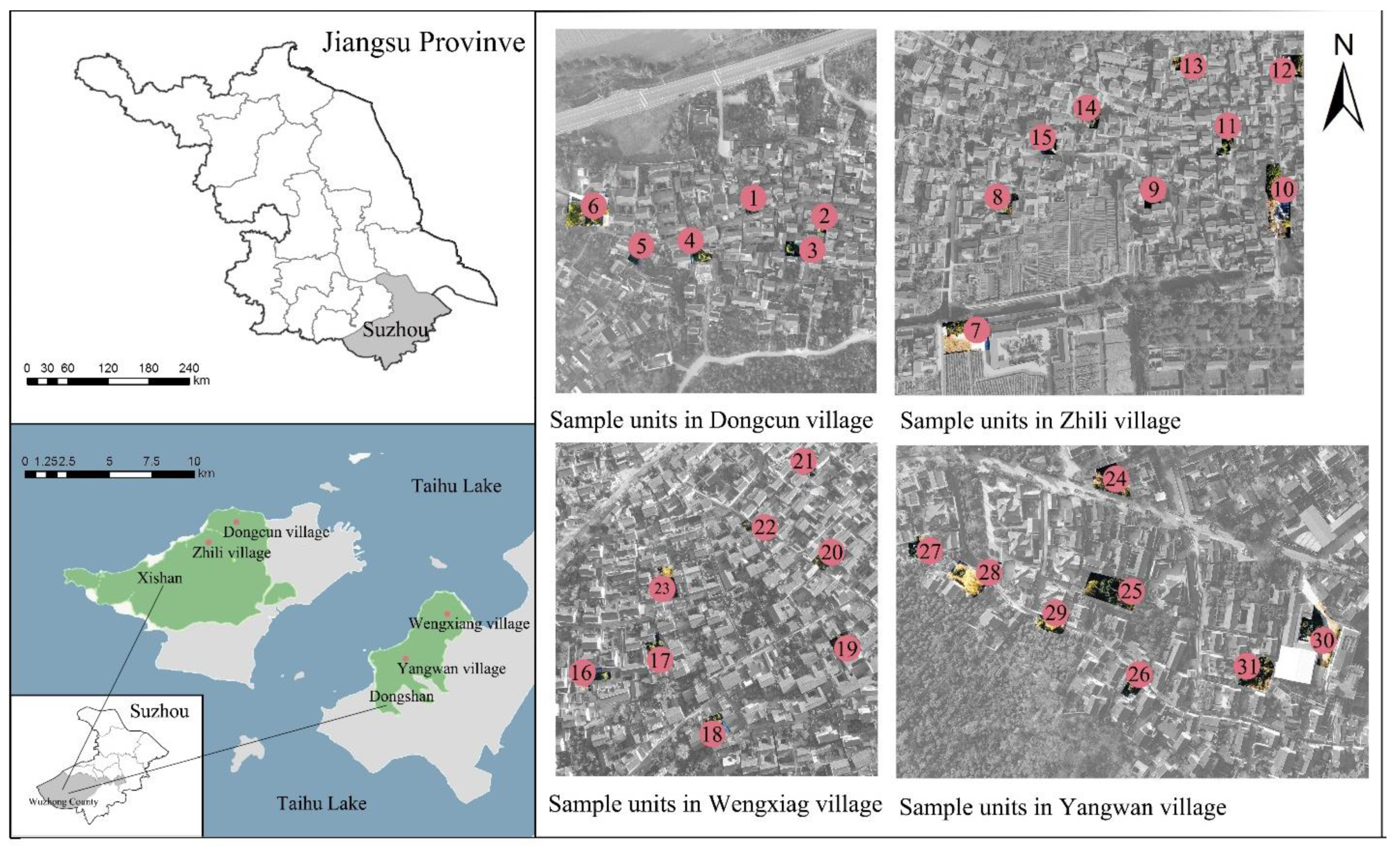
3.1. Research Area

Dongshan and Xishan are ancient towns, located on the east bank of Taihu Basin and west of Suzhou City. The region has a long history and the largest number and greatest concentration of traditional villages in Jiangsu Province. Dongshan is a peninsula extending into Taihu Lake, surrounded by water on three sides, with a total area of approximately 96 km2. In 2017, it had a permanent population of approximately 58,000. Xishan is an island in Taihu Lake, with an area of approximately 83.42 km2. In 2017, it had a population of approximately 45,600 people. The area has a subtropical monsoon humid climate. Coupled with the adjustment effect of Taihu Lake, it has warm and humid micro-climate characteristics, four distinct seasons, sufficient rainfall, and suitable light. The vegetation layers of Dongshan and Xishan are clear. At the highest altitude is a mixed area of conifers and broad-leaved trees and the foothills contain fruit forests and crop planting areas. Due to their pleasant climate, beautiful environment, rich historical relics, and deep cultural heritage, Dongshan and Xishan attract both domestic and international tourists. Yangwan Village, Wengxiang Village, Dongcun Village, and Zhili Village, four representative traditional villages at the national level, were selected as the objects of this research. Yangwan Village has a permanent population of more than 3600 people, Wengxiang Village has approximately 1000 residents, Dongcun Village has approximately 700, and Zhili Village has approximately 400. Field research was conducted during the COVID-19 pandemic, meaning that the villages experienced no tourist activity. Therefore, as an alternative, we interviewed the villagers to establish the main outdoor spaces for daily activities and where tourists congregate. At the same time, informed by the basic theory of space enclosure, we chose 31 typical public space plots to survey and map (Figure 1). These sample sites are public spaces that feature plant landscapes and flat terrain, with boundaries defined by forest edge, curbs or wall foot lines. Among the 31 plots, the smallest area was 90 m2, the largest 1550 m2, and the average area was 661 m2. These space types included parks, playgrounds, squares, and plazas.

3.2. Data Collection and Analysis Methods

The research method used in this study can be divided into the following four main steps (Figure 2). The first step was to quantify the spatial morphological characteristics of the sample plots, survey and map the sample plots with a 3D laser scanner, construct a traditional village public space morphological characteristic index system, preprocess the original point cloud data, and then calculate the value of each index. The second step was to evaluate the landscape aesthetic preference of the sample plot through the beauty degree evaluation method and obtain the beauty degree score of each site. The third step was index screening, which was performed through folding and cross validation, principal component analysis, and full subset regression analysis to screen out suitable morphological indicators. The last step was to fit the selected morphological indicators and beauty degrees according to four different models, which allowed the beauty degree prediction function.

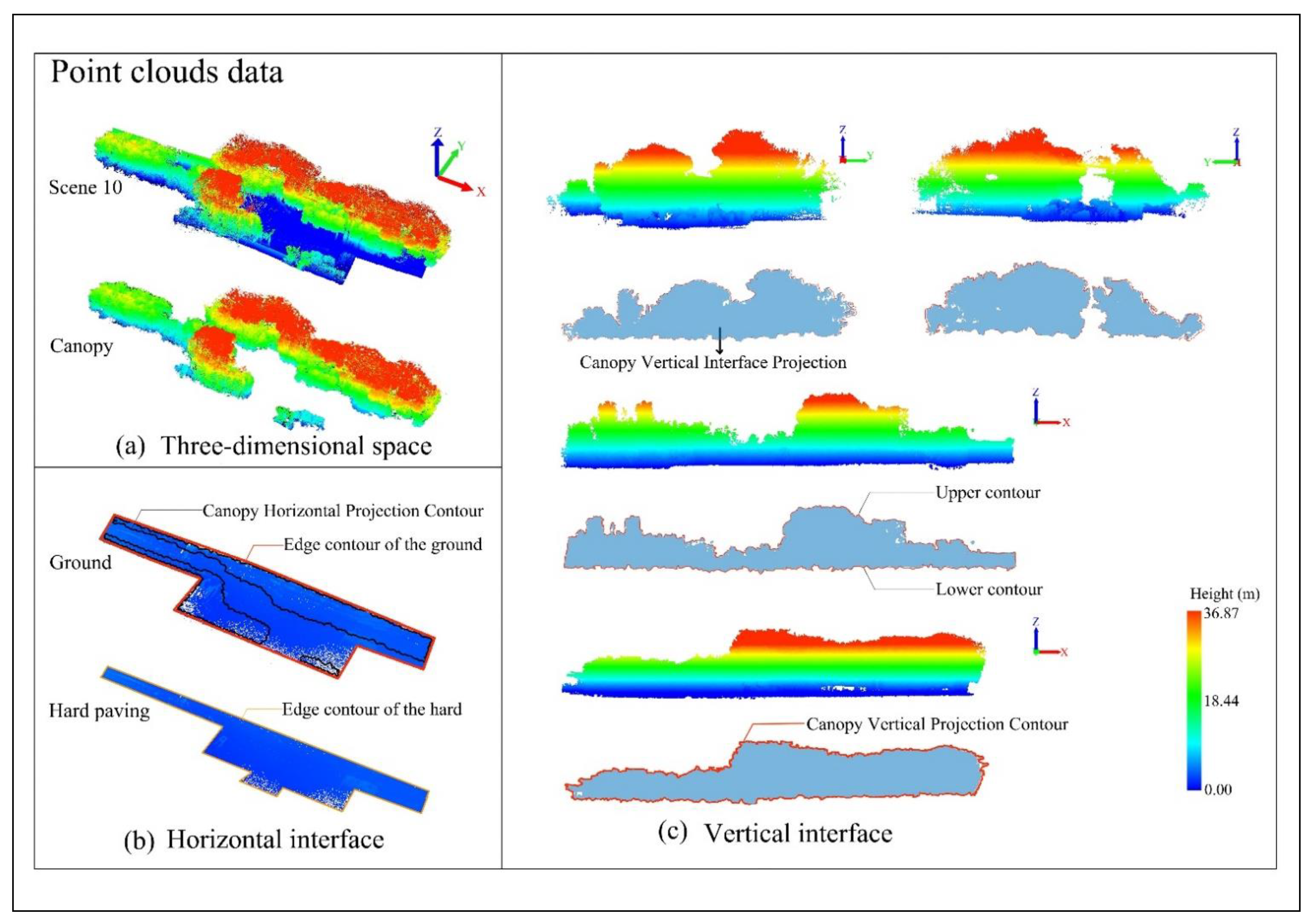
3.2.1. Quantification of Spatial Morphological Characteristics

(1) Surveying and mapping of sample sites
A GEOSLAM ZEB-Horizon handheld 3D laser scanner was used. Unlike airborne and vehicle-mounted radar equipment, this scanner is portable, less affected by weather conditions, and adaptable to traditional village operating environments. With 100 m measuring range and 3 cm scanning accuracy, it meets the accuracy requirements for calculating spatial morphological indicators, as required by this research. The operation method of this instrument is to hold the scanner in front of the chest and circle the field at a normal pace to form a closed loop to complete the scan. Data were collected from 23–25 November 2021.
(2) Establishing the spatial morphological characteristic index system
Factors limiting spatial forms include the bottom-surface factor, vertical interface factor, and top-surface factor [50,52], corresponding to the base plane, vertical separation plane, and covering surface of village landscape space. The combination of these three dimensions forms different spatial types. The base plane of rural landscape space is primarily composed of ground. Divided by pavement, green space, and bodies of water, the size, complexity, and length of the base plane all affect viewers’ visual perceptions. Referencing the quantitative indicators of street space, architectural space, and the base plane of garden plant space, this study used accessible area ratio (AAR), eccentricity (E) [53], and spatial shape index (SSI) [54] as the quantitative indicators of flat spatial forms. The vertical partition surface of village public space is primarily created by the exterior walls of buildings and plant façades. This not only determines the spatial scope and sense of enclosure, but also shapes the communication between the viewer’s vision and the external environment. Referencing the quantitative indicators of the façade forms of street space, waterfront space, and garden plant space, we selected average height of upper contour (hu), average height of lower contour (hl), solid-space ratio (SVR) [55], contour fluctuation range (FR), fluctuation variance of upper contour (FVU), and fluctuation variance of lower contour (FVL) [56,57] as quantitative indicators of façade forms. The top-surface factors of rural public space are primarily formed by the sky and by tree canopy coverage, which affects the height and degree of spatial enclosure. Therefore, in this study, vegetation coverage (VC) [32] was used as the quantitative index of top-surface forms. Base plane, vertical partition plane, and covering surface comprise the landscape space unit. The combination of these three creates a new integrated spatial experience. Based on other types of spatial studies and characteristics of rural landscape space, this study selected the plant diversity index (PDI) [58], 3D-GVI [59], enclosure degree (ED), and comprehensive closure (CC) [50] as the quantitative indicators of three-dimensional spatial forms. According to the definitions of these indicators, the 14 quantitative spatial indicators can be divided into three categories—horizontal interface quantification indicators, vertical interface quantification indicators, and quantification indicators of three-dimensional spatial forms, as shown in Table 1.
(3) Point cloud data preprocessing
Clipping, denoising, ground point extraction, and normalization of point cloud data were conducted to reduce the number of point clouds while preserving the relevant point clouds in the study area. Lidar360 v 3.2 software (Green Valley Team, Beijing, China) was used in this process. Necessary research objects were reserved during clipping, and hard paving decorative cloud and canopy point cloud were separately clipped for later calculation. Human activities, birds, and equipment interfering with the process and the acquired point cloud data were inevitably mixed with other outlier points, namely noise points. These noise points would otherwise impact data processing, reduce data accuracy and perhaps change the final result. We took the distance between points as the primary measurable indicator. Based on multiple experiments, with 10 points as a neighborhood, the median and standard deviation of the mean distance between points in the domain were calculated. We used a calculation formula to determine the maximum threshold of the distance. Points larger than the threshold were considered noise points, and points within the threshold were retained for subsequent calculation. The calculation formula is:
Tmax = M10 + 5 × σ
where T m a x is the threshold of the 10 points,   M is the median of the 10 points, and σ is the standard deviation of the 10 points.
Following pretreatment, the number of point clouds in each sample site reached tens of millions. Such a data redundancy greatly slowed down subsequent data processing. In order to improve computing efficiency, we reduced the number of point clouds by down-sampling. After several attempts, we set the box grid filer at 0.1 m for filtering. The resulting down-sampling brought the point cloud in each sample site down to within half a million.
(4) Spatial morphological indicator calculation
When calculating the above-mentioned morphological indicators, plant diversity indicators were determined using visual interpretation and field investigation. Other morphological indicators that could not be measured directly were calculated using Lidar360 v 3.2 software and R Programming language (R Core Team, Vienna, Austria). The accessible area point cloud was projected onto the XOY plane. Conducting an edge extraction of the point cloud, the edge contour was delineated and the area inside the contour (Aa) was calculated (Figure 3b). We projected the point cloud of the study area onto the XOY plane. By virtue of edge extraction, we outlined the edge contour and calculated the area (Ab) and perimeter (P) in the contour (Figure 3b). We used the traversal method to calculate the Euclidean distance between points, reserving the maximum value as Lmax. We calculated the length of point cloud on the X-axis and Y-axis of the study area, selecting the minimum value as Lmin. We projected the tree canopy point cloud onto the XOY plane, outlining the canopy edge and calculating the contour area through edge extraction of the point cloud. We also used the α-shape method to construct a convex hull for canopy point cloud, with the empirical value of α being 0.03 m, followed by a calculation of the volume of each convex hull, which added up to Vp (Figure 3a). For vertical interface indicators, we first calculated the center point, P0(x0,y0,z0), of the study area, taking Line 1 (xi,y0,zi) and Line 2 (x0,yi,zi), which pass through point P0 and are parallel to the X-axis and Y-axis, respectively, as the threshold values, and partitioning the point cloud in the study area by plane. After calculating indicators of the four partitions, the mean value of the indexes was taken as the indicator of the research area. Then, we projected the partitioned point cloud onto the threshold surface, outlining the edges by virtue of edge extraction of the point cloud, which were output as raster data for the calculation of the contour area (Sp) and the circumference of the upper contour (Pu) (Figure 3c). For h ¯ and h ¯ especially, we calculate the height of the edge inside each grid by the number of columns in the edge grid image and calculated the average height in the contour by integrating and averaging.

3.2.2. SBE Evaluation

(1) Image data collection
In this study, an Insta360 ONE X2 panorama camera was used to take panoramic shots. The main acquisition strategy is as follows: (1) minimize the influence of external environmental factors on the aesthetics of panoramic photos; and (2) ensure that the scene captured by the panoramic image is consistent with the spatial form of scanning and mapping. The shooting height was set as 1.6 m (average adult viewpoint height), and the shooting position was in the center of the scene, so that panoramic photos could fully show the morphological characteristics of the spatial unit. To minimize the impact of climate, temperature, season, and light on spatial appearance, and to ensure that the spatial morphological characteristics displayed in the panorama were consistent with those in the survey and mapping, panoramic shots were taken synchronously with 3D laser scanning mapping and were completed in three days from 23–25 November 2021, during a period of similar weather conditions. Panoramic shooting was conducted from 9:30 am to 11:30 am and from 2:00 pm to 4:00 pm to ensure similar lighting conditions.
(2) Evaluation process
Except for extreme landscapes, there is no statistically significant difference in aesthetic preferences between different groups or people from different cultural backgrounds [40]. This research gave comprehensive consideration to the evaluators’ abilities to operate VR equipment and sought to ensure that landscape rating was not influenced by the personal aesthetics of the evaluators, and selected 40 evaluators composed of landscape architecture postgraduates and people with doctorate degrees and 24 experts (including 14 associate professors, 5 professors and 5 senior engineers) as evaluation subjects. Each evaluator went alone into a room equipped with the devices needed for the evaluation. They were shown the video data and informed of the evaluation procedure and scoring method. A 5-level evaluation scale was used, with the corresponding score ranging from 1 to 5, indicating dislike very much, dislike, neutral, like, and like very much. Participants wore VR glasses (VIVE-VR) to watch the panorama and to score the scenic beauty according to their feelings (Figure 4).
(3) Data processing
Assuming a normal distribution of the evaluation score for each scene, we calculated the average Z value of each scene according to the formula, selected one spatial unit as the reference line to calculate the average Z-value difference between each scene and the reference line, and multiplied the difference by 100 to obtain the original SBE of each scene. The specific calculation steps are as follows:
MZi = 1 m 1 k = 2 m f ( C P i k )
where MZi is the average Z value of the scenic environment; CPik is the cumulative frequency at which the evaluators considered the SBE to be at or above K, when P = 1 or CP = 0, CP = 1 − 1/(2N) or CP = 1/(2N); f (CPik) is the unilateral quantile of normal distribution. In this study, NORMSINV in EXCEL (Microsoft, Redmond, WA, USA) was used for the calculation; m is the total number of grades evaluated; and k is the evaluation grade (1–5).
SBEi = (MZi − BMMZ) ×100
where SBEi is the original SBE of scene i; MZi the average Z value of scene i; and BMMZ the average Z value of the base line of the evaluation object.

3.2.3. Statistical analysis

(1) Index selection
Correlation between each indicator and SBE were analyzed, coupled with classification analysis of all indicators from the horizontal interface, vertical interface, and three-dimensional space. The appropriate number of indicators for model construction was obtained through folding and cross validation. Based on principal component analysis, indicators with a higher contribution rate were selected. Finally, the most suitable indicators were found according to a full subset regression.
(2) Model building and accuracy evaluation
According to the screened indicators, we divided all scenes into training scenes and test scenes. We randomly selected 20 scenes as training scenes for modelling, and all 31 scenes were used to verify model accuracy. We selected and constructed the linear model, nonlinear model, machine learning model, and neural network model. Parameters of the linear model were solved by virtue of the least square method. The exponential function model and polynomial equation model based on response surface analysis were empirically selected for the nonlinear model. As a common classifier of machine learning, random forest is often used for sample training and prediction. It has good prediction accuracy even when the relationship between parameters and sample values is more complex [60]. Neural network processes distribute parallel information by imitating the behavior characteristics of animal neural networks. The BP neural network, a multilayer feedforward neural network trained by an error backward propagation algorithm, is one of the most widely used neural network models [61]. The models are listed in Table 2.
The precision rate (Pr), determination coefficient (R2), and root-mean-square error (RMSE) were used to judge model accuracy. The formulae are as follows:
Pr = P c o r r e c t 11 × 100 %
R 2 = 1 i = 1 31 ( x i x ^ i ) 2 i = 1 31 ( x i x ¯ ) 2
R M S E = 1 31 i = 1 31 ( x i x ^ i ) 2
where Pcorrect is the number of SBEs correctly predicted; x i is the SBE of the ith scene obtained by the calculation; x ^ i is the SBE based on the feature model; and x ¯ is the average SBE of all scenes.

4. Results

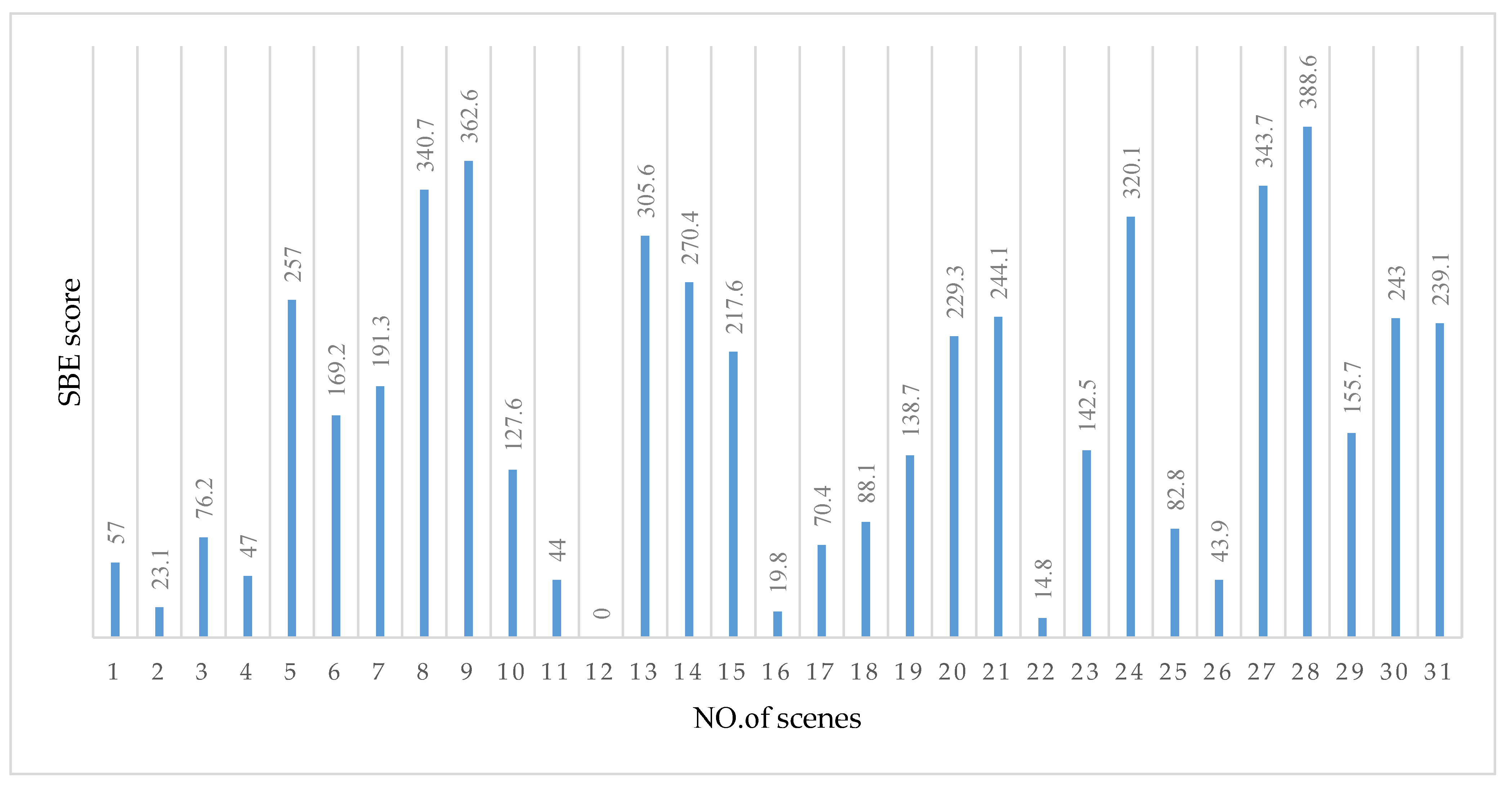
4.1. SBE Evaluation Result

The specific score of the SBE is shown in Figure 5. From high to low, the order is S28 > S9 > S27 > S8 > S24 > S13 > S14 > S5 > S21 > S30 > S31 > S20 > S15 > S7 > S29 > S23 > S19 > S10 > S18 > S25 > S3 > S17> S1 > S4 > S11 > S26 > S2 > S16 > S22 > S12. The extremum method was used to visually represent the SBE of each scene. Scores corresponding to grade 1–5 were calculated using the above formula. The SBE score interval corresponding to the interval of “dislike very much and dislike” was [−40.1, 80.8]; that corresponding to the interval of “dislike and neutral” was [80.8, 201.7]; that corresponding to the interval of “neutral and like” was [201.7, 322.6]; and that corresponding to the interval of “like and like very much” was [322.6, 443.5]. S28, S29, S27, and S8 were between “like and like very much”, S24, S13, S14, S5, S21, S30, S31, S20, and S15 were between “neutral and like”, S7, S29, S23, S19, S10, S18, S25, and S3 were between “dislike and neutral”, and S17, S1, S4, S11, S26, S2, S16, S22, and S12 were between “dislike very much and like”. The average SBE score for public space in Wengxiang Village and Yangwan Village, between “neutral and like,” was higher than that of the other two villages. However, the average SBE score for Wengxiang Village and Yangwan Village was some distance behind “like very much,” demonstrating that all four ancient villages have room for improvement.

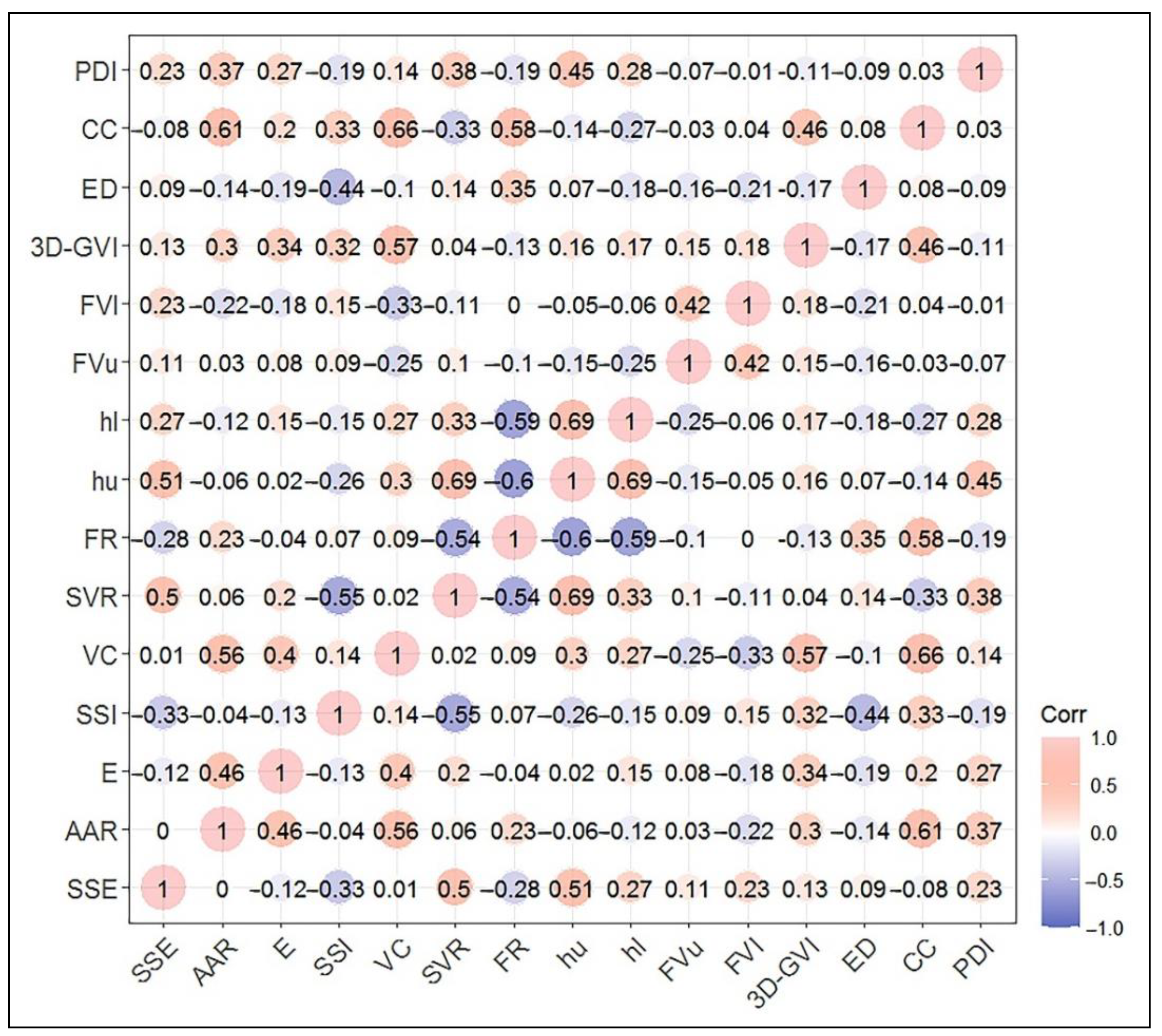
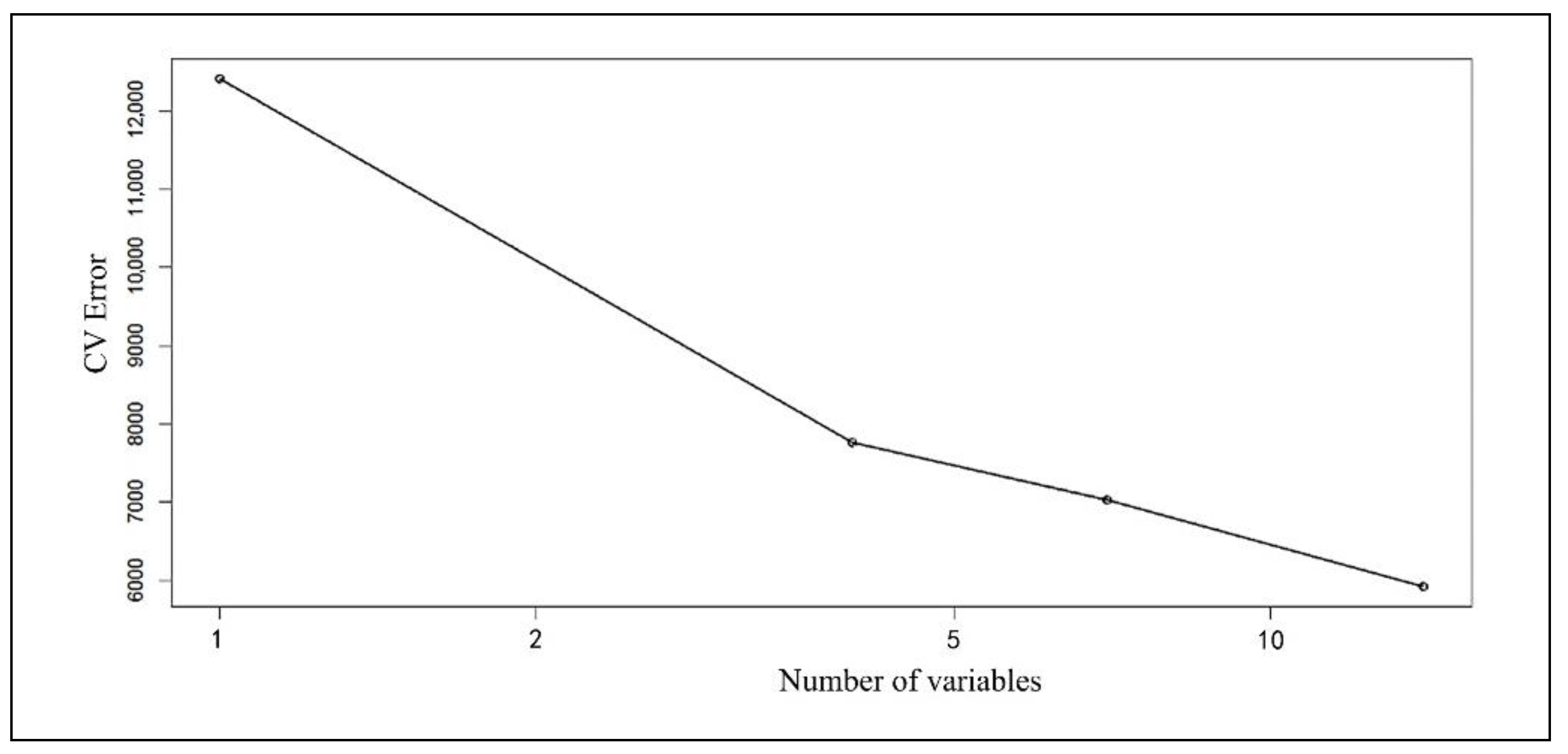
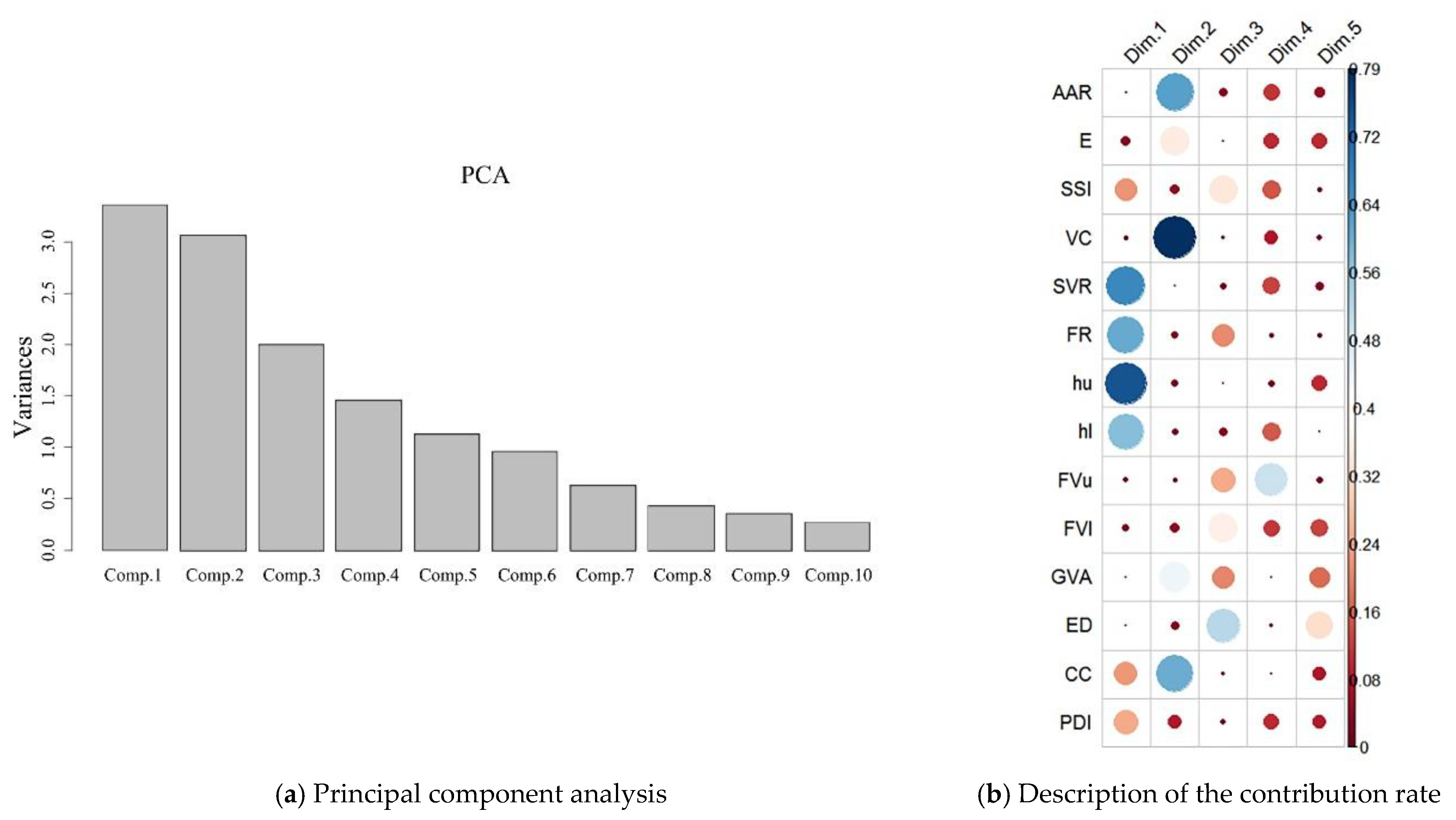
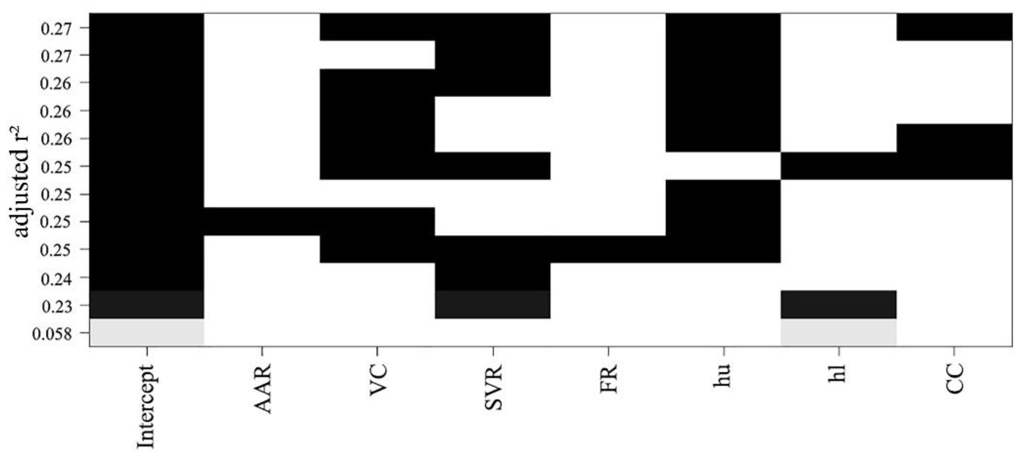
4.2. Parameter Screening

In this study, a correlation analysis of 14 spatial morphological characteristics and the SBE scores for 31 sample environments (Figure 6) show that vertical interface indicators had the greatest correlation with SBE among the three indicator levels. SVR and HU were strongly correlated with SBE value, with the correlation reaching 0.5. The correlation coefficients of spatial shape indicator (SSI), contour fluctuation range (FR), average height of lower contour (hl), fluctuation variance of lower contour (FVl), and plant diversity indicator (PDI) were above 0.2, showing a moderate correlation. Some indicators of horizontal interface and three-dimensional space were weakly correlated with SBE, and correlations between AAR, ED, CC, and SBE were less than 0.10. Weak correlation indicators will not be analyzed as the main research object in a follow-up study.
To ensure that the number of screening parameters was scientific, the influence of preserving different numbers of parameters on model accuracy was calculated according to 10-fold cross verification (Figure 7). This indicates that when the number of parameters is 4, there is an obvious turning point in the model error, meaning that the model error has reached its peak. Therefore, four indicators were selected as parameters for the subsequent model fitting.
Principal component analysis was carried out on indicators to reduce parameters and dimensions and to examine the contribution rates of indicators in different principal components (Figure 7). Significantly, the first principal component and the second principal component present more than 60% of the information (Figure 8a). Therefore, we only considered the index contribution rates in the first and second principal components. A description of the contribution rate of each indicator shows (Figure 8b) the seven indicators circled in blue, meaning they make a greater contribution within their respective principal components. Finally, seven indicators, AAR, VC, SVR, FR, hu, hl, and CC were screened.
These seven indicators were re-screened to decide on four indicators capable of higher model accuracy. A full subset regression analysis of the seven indicators (Figure 9) found that retaining four indicators, VC, SVR, hu, and CC, provided better accuracy, with the adjusted R2 reaching 0.272. We ultimately chose these four indicators.

4.3. Validation of Model Accuracy

Firstly, we established models and calculated the parameters of each model (Table 3), and the calculated object was the SBE score. We divided the predicted SBE score into grades, using the divided grades as a reference to verify the accuracy of each model. Noticeably, considering the accuracy of the random forest model and neural network model, that SBE grade was input as data, and the SBE grade of the scenes was directly predicted. For other models, the SBE score was the main input data. Model evaluation was conducted to judge the accuracy of the SBE grade and to evaluate the accuracy of the SBE score.
As the statistical results in Table 3 show, the linear model and random forest model show excellent prediction capability for SBE grade evaluation. Of the 31 scenes, Pr of the linear model was 70.97% and Pr of the random forest model was 64.52%, which was slightly smaller than the former. This shows that these two models are consistent with the SBE rating system. Among nonlinear models, the exponential function model shows the best Pr (58.06%). The accuracy of the multinomial model and the neural network model was 48.39%, the lowest among all models.
In addition, we evaluated the ability of all models to directly predict the SBE score (Table 4). This shows that all models have low accuracy for direct evaluation of SBE scores. We suspect that this may be due to insufficient sample data. This study, however, found the results of each model to be representative. Of all the models, the random forest model has the best prediction accuracy (R2 = 0.405, RMSE = 63.311). It also has the best result in terms of SBE score. The linear model is the second most accurate for SBE (R2 = 0.332, RMSE = 64.774), followed by the neural network model (R2 = 0.251, RMSE = 95.140) and the polynomial model (R2 = 0.257, RMSE = 117.800). The exponential function model had the worst accuracy (R2 = 0.187, RMSE = 119.517).
In short, both the linear model and the random forest model performed well in SBE grade evaluation and score prediction. The linear model is more suitable for SBE grade evaluation, and the random forest model is more accurate in SBE score prediction.

5. Discussion

5.1. Application Advantages of Handheld 3D Laser Scanners in Traditional Village Surveying and Mapping

As an active remote sensing technology, laser scanning is suitable for basic data collection, processing, and visualization at a variety of spatial scales. However, it is rarely used in the field of landscape architecture for surveying and mapping of micro-scale spaces. Wang et al. [50] quantified the form of 35 open spaces in 5 city parks in the Netherlands and explored the relationship between spatial form and beauty. The data source was the Current Dutch Elevation (AHN3) map and point cloud data were collected from 2014 to 2019, with large differences in the shooting time of the environment evaluation photos. Due to the dynamic characteristics of plant landscapes, differences between the spatial form shown in the photo and the spatial form presented by point cloud data can affect the accuracy of the research results. In this study, a handheld laser scanner was used to effectively solve this problem. The collection of point cloud data and the shooting of spatial images were carried out simultaneously to ensure that the spatial form displayed by the VR panorama was consistent with the spatial form presented by the point cloud data, and point cloud data accuracy was also improved, from 0.5 m to 0.03 m. In order to further verify the advantages of laser scanning technology in the quantitative analysis of traditional village public spaces, we took scene 10 as an example and conducted traditional surveying and mapping of the site on 26 November 2021, making comparisons from four perspectives—operation mode, data accuracy, achievement presentation, and application prospects. Table 5 shows that compared with traditional surveying and mapping, laser scanning technology adopts non-contact scanning, which is less affected by external factors, and which effectively protects the heritage of traditional village cultural landscapes. Handheld 3D laser scanners are portable and can be operated by one individual, which greatly reduces labor and time costs. The accuracy of data collection and analysis is higher than that of manual measurements and, at the same time, the data can be visualized in the form of a three-dimensional space model. The data expression is more intuitive and can be adapted to different quantitative analysis needs.

5.2. Indicator Selection and Model Accuracy

In the process of indicator screening, correlation analysis found that Hu, SVR, SSI, FR, Hl, FVL, and PDI were all correlated with SBE at an over 0.2 absolute value of correlation coefficient, a moderately high correlation. In a further full subset regression analysis, only HU and SVR were involved in the model construction, and the relationship between the other five indicators and the landscape preference score was not obvious. There are two explanations for this. One is that the narrow range of the five indicators in the 31 scene environments makes them incapable of having much of an impact on landscape preference. For example, the interval of FR was only 1.5 and that of PDI was only 1.9. Another explanation may be the relationship between these five indicators and the four indicators involved in model construction; that is, changes in one or several indicators may have led to changes in the remaining indicators.
A large number of previous studies have built models for the prediction of SBE in different scenarios based on a variety of influencing factors [5,44,62]; however, most used a single linear regression model to predict the SBE score. In the actual application process, it is difficult to directly quantify the popularity of the scene environment; only the relative level of beauty of each scene can be obtained, and the relationship between different data cannot be fully explained. In this study, four models were selected to fit the specific scores and grades of SBE, which effectively solved this problem and met different application needs. The random forest model has higher SBE score prediction accuracy and can quickly obtain the relative level of beauty for each scene. The linear model has better SBE grade prediction accuracy, can intuitively represent the popularity of each scene, and can provide guidance for the improvement of traditional village public space landscapes.
After correlation and full subset regression analysis, VC, SVR, hu, and CC were finally screened as having significant impact on predicting the beauty of public spaces in traditional villages in the Lake Taihu area. According to the linear measurement model, hu has positive feedback on SBE. The main elements of the vertical interface of public spaces in traditional villages are plants. Therefore, the average contour height on the vertical interface of a spatial unit reflects the overall plant growth and tree size in that unit. Misgav argues that the physical characteristics of individual plants influence aesthetic preferences, and that increasing plant height is the primary factor in improving landscape quality [63]. Therefore, the average height of the contour on the vertical interface should be in proportion to the size of the trees inside the unit and to the popularity of the scene environment. Our results confirm this. Over the long course of time, traditional villages had large, long-lived trees dotted around their public spaces. Reasonable protection and utilization of this vegetation can effectively improve the quality of the landscape environment. CC has a negative effect on landscape preferences. Openness is viewed as a significant factor influencing scenic beauty preference [64]; spaces with open boundaries, discontinuities, and gaps are more popular than confined spaces [3]. SVR is reflective of the closure of a vertical interface and is an important embodiment of the openness of a scene. The linear model shows that SR is in proportion to the popularity of a scene, contrary to the findings of previous studies [50]. An analysis of the SVR values of 31 landscape spatial units indicates a range between 0.08 and 0.15, which is far smaller than the half-open space preferred by the public (0.5) [9]. The positive feedback between SVR and landscape preference in this study may have been caused by the wide façade enclosure and lack of shelter at the 31 sites. This echoes Appleton’s “prospect-refuge” theory [65], which argues that people wish to see but not to be seen. Vegetation cover in the model may provide negative feedback on landscape preference. A place of greater coverage offers greater privacy. Coming to such a place may arouse feelings of owning the domain. Such a place will lose its appeal if it has to be shared with others. Traditional village public spaces are places for people to relax and communicate, so vegetation coverage should not be too high. Based on the above considerations, planning and management departments should reduce government intervention in the process of traditional village protection and renewal and encourage villagers and tourists to participate in the decision-making process. Starting from the above four indicators, we should enhance the vitality of the public relations space in traditional villages and focus on protecting ancient and famous trees in villages. In addition, the amount of vegetation in the public space should be increased. Attention should be paid to the integration of vegetation and the environment, and taking into account the social function, ecological function and aesthetic function of the public space can maximize the compound benefit.

5.3. Deficiencies and Prospects

This study has some limitations. First, while the experiments limited conditions affecting data acquisition, such as time, weather, and light, there was no way to completely avoid the influence of factors other than spatial morphological characteristics on landscape preference, such as color, texture, and emotion. In the follow-up research, index elements other than morphological indicators will be incorporated, and the selection of morphological indicators will be enriched to promote the refined management of traditional village landscapes. Thirty-one sites were selected for this research, and the function models we obtained were based on the morphological characteristic data and SBE of those thirty-one sites. Each indicator value had a certain range, making it difficult to discuss the relationship between spatial morphological characteristics and landscape preference beyond those numerical ranges. However, follow-up studies can expand the sample size. Second, this study focused on public spaces in traditional villages, the formation of which is shaped by natural and human factors, and obvious regional characteristics. The morphological characteristics of landscaped public space in different regions obviously differ. This research explored traditional villages in Dongshan and Xishan, Lake Taihu, Suzhou. The relationship between the public space characteristics of traditional village landscapes and landscape preferences in other regions requires further exploration. However, this methodology is applicable to other areas.
Third, in order to explore whether model accuracy can be improved, in addition by selecting more models, we started from the perspective of indicators, hoping to improve model accuracy by fusing more relevant indicators. We selected indicators with the highest correlation from the three types of indicators, namely SSI, HU, and PDI. Multiplying any two of these three indicators produces three fused indicators, namely SSI_hu, SSI_PDI, and hu_PDI. Correlation between all indicators, including the three fused indicators, and SBE was calculated, with parameters re-screened to establish the model. When modelling, the linear model was chosen as the basic model according to the findings of this study, with model accuracy verified by predicting SBE and ranking all the sites (Table 6). We found that, although fusion indicators were not very helpful in the evaluation of SBE grade, R2 was significantly improved in predicting the SBE score, suggesting that fused indicators can provide better accuracy for SBE score fitting. In future experiments, more consideration will be given to the influence of fused indicators on model accuracy.

6. Conclusions

In this study, a morphological characteristic index system of traditional village public space at the micro-scale was constructed based on spatial components, and a handheld 3D laser scanner was used to obtain spatial point cloud data, which solved the problem of the lack of spatial data sources at the micro-scale in rural areas. Using VR panoramic instead of traditional photo media to evaluate the beauty of the scene environments made result evaluation more closely resemble on-site scoring. Through correlation analysis and full subset regression analysis, four key indicators of beauty degree prediction were screened, namely hu, SVR, VC, and CC. Taking the four key indicators as variables, the linear model, nonlinear model, machine learning model, and BP neural network model were selected to fit SBE scores and grades. The degree level was found to have better prediction accuracy. The random forest model (R2 = 0.405, RMSE = 63.311) had the best effect on beauty degree score prediction and met different prediction needs. According to the prediction model, of the four key indicators, SVR and hu had positive feedback on scenic beauty preference, while VC and CC had negative feedback on landscape preference. The research offers a good explanation for the aesthetic preferences for public spatial forms in traditional villages in the research area. It thus provides guidance for the protection and renewal of traditional village public spaces in the area and offers management and design as the basis for government and design decision-making. The methods used in this paper to quantify spatial forms and evaluate landscape preference are applicable to studies of different types of landscape space in traditional villages in other regions, as well as research on landscape space in urban environments.

Author Contributions

Conceptualization, G.C.; methodology, G.C.; software, X.S. and W.Y.; validation, G.C.; formal analysis, G.C.; investigation, G.C. and W.Y.; resources, W.Y.; data curation, G.C.; writing—original draft preparation, G.C.; writing—review and editing, G.C.; visualization, X.S.; supervision, H.W.; project administration, H.W.; funding acquisition, H.W. All authors have read and agreed to the published version of the manuscript.

Funding

This research was funded by the “National Key Research and Development Program of China” (grant number 2019YFD1100404): Research on the construction and application technology of rural plant landscape.

Informed Consent Statement

Informed consent was obtained from all subjects involved in the study.

Data Availability Statement

The data presented in this study are available on request from the author. Images employed for the study will be available online for readers.

Conflicts of Interest

The authors declare no conflict of interest.

References

  1. Chhetri, P.; Arrowsmith, C. GIS-based Modelling of Recreational Potential of Nature-Based Tourist Destinations. Tour. Geogr. 2008, 10, 233–257. [Google Scholar] [CrossRef]
  2. Stoltz, J.; Grahn, P. Perceived Sensory Dimensions: An Evidence-based Approach to Greenspace Aesthetics. Urban For. Urban Green. 2021, 59, 126989. [Google Scholar] [CrossRef]
  3. Shulin, S.; Zhonghua, G.; Leslie, H.C. How does enclosure influence environmental preferences? A cognitive study on urban public open spaces in Hong Kong. Sustain. Cities Soc. 2014, 13, 148–156. [Google Scholar]
  4. Howley, P.; Donoghue, C.O.; Hynes, S. Exploring public preferences for traditional farming landscapes. Landsc. Urban Plan. 2012, 104, 66–74. [Google Scholar] [CrossRef]
  5. Schirpke, U.; Tasser, E.; Tappeiner, U. Predicting scenic beauty of mountain regions. Landsc. Urban Plan. 2013, 111, 1–12. [Google Scholar] [CrossRef]
  6. Daniel, T.C. Whither scenic beauty? Visual landscape quality assessment in the 21st century. Landsc. Urban Plan. 2001, 54, 267–281. [Google Scholar] [CrossRef]
  7. Zube, E.H.; Sell, J.L.; Taylor, J.G. Landscape perception: Research, application and theory. Landsc. Plan. 1982, 9, 1–33. [Google Scholar] [CrossRef]
  8. Zube, E.H.; Pitt, D.G. Cross-cultural perceptions of scenic and heritage landscapes. Landsc. Plan. 1981, 8, 69–87. [Google Scholar] [CrossRef]
  9. Tveit, M.S. Indicators of visual scale as predictors of landscape preference; a comparison between groups. J. Environ. Manag. 2009, 90, 2882–2888. [Google Scholar] [CrossRef] [PubMed]
  10. Hermes, J.; Berkel, D.V.; Burkhard, B.; Plieninger, T.; Fagerholm, N.; Haaren, C.V.; Albert, C. Assessment and valuation of recreational ecosystem services of landscapes. Ecosyst. Serv. 2018, 31, 289–295. [Google Scholar] [CrossRef] [PubMed]
  11. Wartmann, F.M.; Purves, S.R. Investigating sense of place as a cultural ecosystem service in different landscapes through the lens of language. Landscape Urban Plan 2018, 175, 169–183. [Google Scholar] [CrossRef]
  12. Hernández, J.; Garca, L.; Ayuga, F. Assessment of the visual impact made on the landscape by new buildings: A methodology for site selection. Landsc. Urban Plan. 2004, 68, 15–28. [Google Scholar] [CrossRef]
  13. Robinson, N. The planting design handbook. Arboric. J. 2011, 35, 59–60. [Google Scholar]
  14. De Vries, S.; De Groot, M.; Boers, J. Eyesores in sight: Quantifying the impact of man-made elements on the scenic beauty of Dutch landscapes. Landsc. Urban Plan. 2012, 105, 118–127. [Google Scholar] [CrossRef]
  15. Hagerhall, C.M.; Purcell, T.; Taylor, R. Fractal dimension of landscape silhouette outlines as a predictor of landscape preference. J. Environ. Psychol. 2004, 24, 247–255. [Google Scholar] [CrossRef]
  16. Liang, H.; Li, W.; Lai, S.; Zhu, L.; Jiang, W.; Zhang, Q. The integration of terrestrial laser scanning and terrestrial and unmanned aerial vehicle digital photogrammetry for the documentation of Chinese classical gardens—A case study of Huanxiu Shanzhuang, Suzhou, China. J. Cult. Heritage 2018, 33, S827726525. [Google Scholar] [CrossRef]
  17. Val, G.; Atauri, J.A.; Lucio, J. Relationship between landscape visual attributes and spatial pattern indices: A test study in Mediterranean-climate landscapes. Landsc. Urban Plan. 2006, 77, 393–407. [Google Scholar]
  18. Kempenaar, A.; Adri, V. Regional designing: A strategic design approach in landscape architecture. Des. Stud. 2018, 54, 80–95. [Google Scholar] [CrossRef]
  19. Guneroglu, N.; Bekar, M. A Methodology of Transformation from Concept to form in Landscape Design. J. Hist. Cult. Art Res. 2019, 8, 243–253. [Google Scholar] [CrossRef]
  20. Treib, M. The content of landscape form [The limits of formalism]. Landsc. J. 2001, 20, 119–140. [Google Scholar] [CrossRef] [Green Version]
  21. Polat, A.T.; Akay, A. Relationships between the visual preferences of urban recreation area users and various landscape design elements. Urban For. Urban Green. 2015, 14, 573–582. [Google Scholar] [CrossRef]
  22. Gobster, P.H.; Ribe, R.G.; Palmer, J.F. Themes and trends in visual assessment research: Introduction to the Landscape and Urban Planning special collection on the visual assessment of landscapes. Landsc. Urban Plan. 2019, 191, 103635. [Google Scholar] [CrossRef]
  23. Wu, C.; Xiao, Q.; Mcpherson, E.G. A method for locating potential tree-planting sites in urban areas: A case study of Los Angeles, USA. Urban For. Urban Green. 2008, 7, 65–76. [Google Scholar] [CrossRef]
  24. Yan, J.; Zhou, W.; Han, L.; Qian, Y. Mapping vegetation functional types in urban areas with WorldView-2 imagery: Integrating object-based classification with phenology. Urban For. Urban Green. 2018, 31, S945842183. [Google Scholar] [CrossRef]
  25. Ren, Z.; Zheng, H.; He, X.; Zhang, D.; Yu, X.; Shen, G. Spatial estimation of urban forest structures with Landsat TM data and field measurements. Urban For. Urban Green. 2015, 14, 336–344. [Google Scholar] [CrossRef]
  26. Gupta, K.; Roy, A.; Luthra, K.; Maithani, S.; Mahavir. GIS based analysis for assessing the accessibility at hierarchical levels of urban green spaces. Urban For. Urban Green. 2016, 19, 198–211. [Google Scholar] [CrossRef]
  27. Margaritis, E.; Kang, J. Relationship between urban green spaces and other features of urban morphology with traffic noise distribution. Urban For. Urban Green. 2016, 15, 174–185. [Google Scholar] [CrossRef]
  28. Zhao, S.M.; Ma, Y.F.; Wang, J.L.; You, X.Y. Landscape Pattern Analysis and Ecological Network Planning of Tianjin City. Urban For. Urban Green. 2019, 46, 126479. [Google Scholar] [CrossRef]
  29. Majumdar, D.D.; Biswas, A. Quantifying land surface temperature change from LISA clusters: An alternative approach to identifying urban land use transformation. Landsc. Urban Plan. 2016, 153, 51–65. [Google Scholar] [CrossRef]
  30. Shukla, A.; Jain, K. Analyzing the impact of changing landscape pattern and dynamics on land surface temperature in Lucknow city, India. Urban For. Urban Green. 2020, 58, 126877. [Google Scholar] [CrossRef]
  31. Zhang, R.; Zhang, L.; Zhong, Q.; Zhang, Q.; Ji, Y.; Song, P.; Wang, Q. An optimized evaluation method of an urban ecological network: The case of the Minhang District of Shanghai—ScienceDirect. Urban For. Urban Green. 2021, 62, 127158. [Google Scholar] [CrossRef]
  32. Fratarcangeli, C.; Fanelli, G.; Franceschini, S.; De Sanctis, M.; Travaglini, A. Beyond the urban-rural gradient: Self-Organizing Map detects the nine landscape types of the city of Rome. Urban For. Urban Green. 2019, 38, 354–370. [Google Scholar] [CrossRef]
  33. Peter, C.M.; Stigaard, L.M.; Nyholm, J.R.; Søren, S.; René, G. Designing and Testing a UAV Mapping System for Agricultural Field Surveying. Sensors 2017, 17, 2703. [Google Scholar]
  34. Kumar, P.B.; Patil, A.K.; Chethana, B.; Chai, Y.H. On-Site 4-in-1 Alignment: Visualization and Interactive CAD Model Retrofitting Using UAV, LiDAR’s Point Cloud Data, and Video. Sensors 2019, 19, 3908. [Google Scholar]
  35. Patrikar, J.; Moon, B.G.; Scherer, S. Wind and the City: Utilizing UAV-Based In-Situ Measurements for Estimating Urban Wind Fields. In Proceedings of the 2020 IEEE/RSJ International Conference on Intelligent Robots and Systems (IROS), Las Vegas, NV, USA, 24 October 2020–24 January 2021. [Google Scholar]
  36. Radoglou-Grammatikis, P.; Sarigiannidis, P.; Lagkas, T.; Moscholios, I. A compilation of UAV applications for precision agriculture. Comput. Netw. 2020, 172, 107148. [Google Scholar] [CrossRef]
  37. Godwin, C.; Chen, G.; Singh, K.K. The impact of urban residential development patterns on forest carbon density: An integration of LiDAR, aerial photography and field mensuration. Landsc. Urban Plan. 2015, 136, 97–109. [Google Scholar] [CrossRef]
  38. Ucar, Z.; Bettinger, P.; Merry, K.; Akbulut, R.; Siry, J. Estimation of urban woody vegetation cover using multispectral imagery and LiDAR. Urban For. Urban Green. 2017, 29, 248–260. [Google Scholar] [CrossRef]
  39. Qiang, Y.; Shen, S.; Chen, Q. Visibility analysis of oceanic blue space using digital elevation models. Landsc. Urban Plan. 2019, 181, 92–102. [Google Scholar] [CrossRef]
  40. Daniel, T.C.; Boster, R.S. Measuring Landscape Esthetics: The Scenic Beauty Estimation Method; Res. Pap. RM-RP-167; U.S. Department of Agriculture, Forest Service, Rocky Mountain Range and Experiment Station: Washington, DC, USA, 1976.
  41. Clay, G.R.; Daniel, T.C. Scenic landscape assessment: The effects of land management jurisdiction on public perception of scenic beauty. Landsc. Urban Plan. 2000, 25, 1–13. [Google Scholar] [CrossRef]
  42. Clay, G.R.; Smidt, R.K. Assessing the validity and reliability of descriptor variables used in scenic highway analysis. Landsc. Urban Plan. 2004, 66, 239–255. [Google Scholar] [CrossRef]
  43. Yao, Y.; Zhu, X.; Xu, Y.; Yang, H.; Xian, W.; Li, Y.; Zhang, Y. Assessing the visual quality of green landscaping in rural residential areas: The case of Changzhou, China. Environ. Monit. Assess 2012, 184, 951–967. [Google Scholar] [CrossRef] [PubMed]
  44. Arriaza, M.; Cañas-Ortega, J.F.; Cañas-Madueño, J.A.; Ruiz-Aviles, P. Assessing the visual quality of rural landscapes. Landsc. Urban Plan. 2004, 69, 115–125. [Google Scholar] [CrossRef]
  45. Rogge, E.; Nevens, F.; Gulinck, H. Perception of rural landscapes in Flanders: Looking beyond aesthetics. Landsc. Urban Plan. 2007, 82, 159–174. [Google Scholar] [CrossRef]
  46. Sevenant, M.; Antrop, M. Cognitive attributes and aesthetic preferences in assessment and differentiation of landscapes—ScienceDirect. J. Environ. Manag. 2009, 90, 2889–2899. [Google Scholar] [CrossRef]
  47. Sun, Y.N.; Zhao, X.; Wang, Y.H.; Li, F.Z.; Li, X. Study on the visual evaluation preference of rural landscape based on VR panorama. J. Beijing For. Univ. 2016, 38, 104–112. [Google Scholar]
  48. Daniel, T.C.; Meitner, M.M. Representational validity of landscape visualizations: The effects of graphical realism on perceived scenic beauty of forest vistas. J. Environ. Psychol. 2001, 21, 61–72. [Google Scholar] [CrossRef] [Green Version]
  49. Hull, R.B.; Stewart, W. Validity of photo-based scenic beauty judgments. J. Environ. Psychol. 2015, 12, 101–114. [Google Scholar] [CrossRef]
  50. Wang, Y.; Zlatanova, S.; Yan, J.; Huang, Z.; Cheng, Y. Exploring the relationship between spatial morphology characteristics and scenic beauty preference of landscape open space unit by using point cloud data. Environ. Plan. B Urban Anal. City Sci. 2020, 48, 1822–1840. [Google Scholar] [CrossRef]
  51. Gao, Y.; Zhang, T.; Sasaki, K.; Uehara, M.; Jin, Y.; Qin, L. The spatial cognition of a forest landscape and its relationship with tourist viewing intention in different walking passage stages. Urban For. Urban Green. 2021, 58, 126975. [Google Scholar] [CrossRef]
  52. Yan, J.; Diakité, A.A.; Zlatanova, S. An extraction approach of the top-bounded space formed by buildings for pedestrian navigation. ISPRS Ann. Photogramm. Remote Sens. Spat. Inf. Sci. 2018, 4. [Google Scholar] [CrossRef] [Green Version]
  53. Parisien, M.; Peters, V.S.; Wang, Y.; Little, J.M.; Bosch, E.M.; Stocks, B.J. Spatial patterns of forest fires in Canada, 1980–1999. Int. J. Wildland Fire 2006, 15, 361–374. [Google Scholar] [CrossRef]
  54. Ode, Å.; Fry, G.; Tveit, M.S.; Messager, P.; Miller, D. Indicators of perceived naturalness as drivers of landscape preference. J. Environ. Manag. 2007, 90, 375–383. [Google Scholar] [CrossRef] [PubMed]
  55. Casey, E.S. The Edge(s) of Landscape: A Study in Liminology. In The Place of Landscape: Concepts, Contexts, Studies; The MIT Press: Cambridge, MA, USA, 2011; pp. 99–109. [Google Scholar]
  56. Jakobsen, P. Shrubs and Groundcover. In Landscape Design with Plants; CRC Press: Boca Raton, FL, USA, 1990. [Google Scholar]
  57. Wöhrle, R.E.; Wöhrle, H.J. Basics Designing with Plants; Birkhäuser: Basel, Switzerland, 2008. [Google Scholar]
  58. Amaral, L.; Ferreira, R.A.; Lisboa, G.; Longhi, S.J.; Watzlawick, L.F. Variabilidade espacial do Índice de Diversidade de Shannon-Wiener em Floresta Ombrófila Mista. Emilio Montero Cartelle 2013, 1961–1972. [Google Scholar]
  59. Zheng, S.; Meng, C.; Xue, J.; Wu, Y.; Liang, J.; Xin, L.; Zhang, L. UAV-based spatial pattern of three-dimensional green volume and its influencing factors in Lingang New City in Shanghai, China. Front. Earth Sci. 2021, 15, 543–552. [Google Scholar] [CrossRef]
  60. Svetnik, V. Random forest: A classification and regression tool for compound classification and QSAR modeling. J. Chem. Inf. Comput. Sci. 2003, 43, 1947–1958. [Google Scholar] [CrossRef]
  61. Zhi, X.; Ye, S.-J.; Zhong, B.; Sun, C.-X. BP neural network with rough set for short term load forecasting. Expert Syst. Appl. Int. J. 2009, 36, 273–279. [Google Scholar]
  62. Fathi, M.; Masnavi, M.R. Assessing Environmental Aesthetics of Roadside Vegetation and Scenic Beauty of Highway Landscape: Preferences and Perception of Motorists. Int. J. Environ. Res. 2014, 8, 941–952. [Google Scholar]
  63. Misgav, A. Visual preference of the public for vegetation groups in Israel. Landsc. Urban Plan. 2000, 48, 143–159. [Google Scholar] [CrossRef]
  64. Kaplan, S. Aesthetics, Affect, and Cognition: Environmental Preference from an Evolutionary Perspective. Environ. Behav. 2016, 19, 3–32. [Google Scholar] [CrossRef] [Green Version]
  65. Appleton, J. Prospects and Refuges Revisited. Landsc. J. 1984, 3, 91–103. [Google Scholar] [CrossRef]
Figure 1. Thirty-one sample sites in four traditional villages.
Land 11 01133 g001
Figure 2. Technical flowchart.
Land 11 01133 g002
Figure 3. Schematic diagram of indicator calculation.
Land 11 01133 g003
Figure 4. Scenic beauty evaluation.
Land 11 01133 g004
Figure 5. SBE score of each scene.
Land 11 01133 g005
Figure 6. Results of correlation analysis.
Land 11 01133 g006
Figure 7. Ten-fold cross verification.
Land 11 01133 g007
Figure 8. Principal component analysis (PCA).
Land 11 01133 g008
Figure 9. Full subset regression analysis.
Land 11 01133 g009
Table 1. Quantitative index system of traditional village public space form.
Spatial CompositionQuantitative IndicatorsIndicator DefinitionComputational Formula
Horizontal interfaceAccessible area ratio (AAR)Representing the proportion of the area accessible to viewers of a spatial unit; the larger the value, the larger the area that can be accessed by viewers per unit areaAAR = Aa/Ab
Aa stands for the accessible area of a spatial unit, and Ab the base area of a spatial unit
Eccentricity (E)Representing the length and width of a spatial unit, the larger the value, the longer and narrower or shorter and wider the space.E = Lmax/Lmin
Lmax is the long axis length of the bottom surface of a spatial unit, while Lmin the broken axis length of the bottom surface of a spatial unit
Spatial Shape Index (SSI)Representing the complexity of the bottom surface of a spatial unit. The closer the index is to 1, the closer the bottom surface of the spatial unit is to a circle SSI = p 2 / 4 π A b  
p is the base perimeter of a spatial unit, and Ab the base area of the spatial unit
Vegetation coverage (VC)Proportion of vertical projection area of vegetation inside a spatial unit; the closer the value is to 1, the higher the green coverage rate in the spatial unitVC = Sveg/Ab
Sveg is the vertical projection area of vegetation in the spatial unit, and Ab the bottom area of the spatial unit
Vertical interfaceAverage height of upper contour (hu)Average height of upper contour of vertical interface of a spatial unit hu = 1 N i = 1 N h i
hi is the height of the ith point of the contour on the vertical interface of the spatial unit
Average height of lower contour (hl)Average height of lower contour of vertical interface of a spatial unit hl = 1 N i = 1 N h i
hi′ is the height of the ith point of the lower contour on the vertical interface of the spatial unit
Solid-space ratio (SVR)Proportion of vertical projection area of vegetation in a spatial unit, the closer the value is to 1, the higher green coverage rate in the spatial unitSVR = SP/(hmax × P)
SP is the area occupied by the vertical interface of the entity elements, hmax the maximum height of the contour on the vertical interface, and P the underside perimeter of the spatial unit
Contour fluctuation range (FR)Representing the fluctuation of the upper contour of the entity elements of the vertical interface. The closer the value is to 1, the more uniform the contour height changes on the vertical interface of the spatial unitFR = hmax/hu
hmax is the maximum height of the contour on the vertical interface of the spatial unit, hu the average height of contour on a vertical surface of the spatial unit
Fluctuation variance of upper contour (FVU)Representing the intensity of fluctuation of the upper contour of the vertical interface. The larger the value, the more intense the fluctuation of the contour height on the vertical interface of the spatial unit FVU = 1 N i = 1 N   ( hi hu )  
hi is the height of the ith point of the contour on the vertical interface of the spatial unit, hu the average height of contour on the vertical plane of the spatial unit
Fluctuation variance of lower contour (FVL)Representing the intensity of the fluctuation of the lower contour of the vertical interface. The larger the value, the more intense the fluctuation of the lower contour height on the vertical interface of the spatial unit FVL = 1 N i = 1 N   ( hi hl )  
hi′ is the height of the ith point of the lower contour on the vertical interface of the spatial unit, hl the average height of lower contour on the vertical interface of the spatial unit.
Three-dimensional spacePlant diversity Index (PDI)Representing the richness of vegetation in a spatial unit; the greater the value, the more diverse the plants PDI = i = 1 S P i ln P i
Pi = Ni/N, Ni is the number of individuals of species i, i = 1, 2, 3, …S, N is the total number of individuals
3D-green view index(3D-GVI)Volume of tree cover in a spatial unit; the larger the value, the larger the proportion of plants in a spatial unit3D-GVI = Vp/(hmax × Ab)
Vp is the volume of vegetation in a spatial unit, hmax the maximum height of contour on the vertical interface of the spatial unit, Ab the base area of the spatial unit
Enclosure degree (ED)Representing the enclosure of a spatial unit, and the higher the value, the higher the enclosureED = PU/P
PU is the perimeter of the upper contour on the vertical interface of a spatial unit, P the underside perimeter of the spatial unit
Comprehensive closure (CC)Representing the combined enclosure of a spatial unit; the larger the value, the higher the enclosure of the spatial unitCC = Sv/Ab
Sv is the area of interface between the upper contour and lower contour on the vertical interface of the spatial unit, Ab the bottom area of the spatial unit
Table 2. Model list.
ModelsTypesFunctions
LinearLeast Squares Y = p 1 x 1 + p 2 x 2 + p 3 x 3 + p 0
NonlinearExponential Function E X P ( p 1 x 1 p 2 x 2 + p 0 )
Polynomial Function a x 1 2 + b x 1 x 2 + c x 2 2 + d
Machine LearningRandom ForestR package randomForest
Neural NetworkBack PropagationR package nnet-
Table 3. Model parameter calculation and model establishment.
ModelsTypesFunctions/Parameters of ModelsNumber of Correct GradesPr
LinearLeast Squares S B E = 27.406 V C + 8500.683 S V R + 7.18 h u 3.225 C C 14.51 2270.97
NonlinearExponential Function E X P ( 0.02 V C + 70.135 S V R + 0.086 h u 1.106 C C + 3.138 ) 1858.06
Polynomial Function a x 1 2 + b x 1 x 2 + c x 2 2 + d 1548.39
Machine LearningRandom ForestImport Parameters: VC, SVR, hu, CC
Import Labels: SBE/Grades of SBE
Iterations: 1000
2064.52
Neural NetworkBack PropagationImport Parameters: VC, SVR, hu, CC
Import Labels: SBE/Grades of SBE
Iterations: 1000
Layers: 5
1548.39
Table 4. Ability of all models to directly predict SBE score.
ModelsTypesR-SquareRMSE/Score
LinearLeast Squares0.33264.774
NonlinearExponential Function0.187119.517
Polynomial Function0.257117.800
Machine LearningRandom Forest0.40563.311
Neural NetworkBack Propagation0.25195.140
Table 5. Comparison of laser scanning technology and traditional surveying and mapping.
Scene10 (419.39 m2)3D Laser Scanning TechnologyTraditional Mapping
Assignment styleEquipment: handheld laser scanner (GEOSLAM ZEB-Horizon)
Non-contact scanning, less interference from external factors
Time Consumption: 12 min for a single person
Equipment: tape measure, perimeter, digital camera
Contact measurement, greatly disturbed by external factors
Time consumption: 2 h for 3 people
Data precisionRange: 100 m, Relative accuracy: 1.5–3 cmMore random
Results presentation3D model
Data processing time: 28 min for a single person
2D photos, reports
Data processing time: 5 h for 2 people
Application prospectQuantitative analysis of three-dimensional space morphology, microclimate simulation, auxiliary scheme design2D interface analysis
Table 6. Model accuracy verification.
Number of ParametersModelsNumber of Correct GradesPrR-Square
14Linear2270.970.332
17 (including 3 mixed parameters)Linear2270.970.392
Publisher’s Note: MDPI stays neutral with regard to jurisdictional claims in published maps and institutional affiliations.

