Article

Spatiotemporal Change Analysis and Prediction of Future Land Use and Land Cover Changes Using QGIS MOLUSCE Plugin and Remote Sensing Big Data: A Case Study of Linyi, China

1
School of Information Science and Engineering, Linyi University, Linyi 276000, China
2
School of Geography, South China Normal University, Guangzhou 510631, China
3
Institut de Géographie Alpine (IGA), Université Grenoble Alpes, 38100 Grenoble, France
*
Author to whom correspondence should be addressed.
Land 2022, 11(3), 419; https://doi.org/10.3390/land11030419
Submission received: 14 February 2022 / Revised: 9 March 2022 / Accepted: 10 March 2022 / Published: 14 March 2022

Abstract

:
Land use and land cover (LULC) change analysis is a systematic technique that aids in the comprehension of physical and non-physical interaction with the natural habitat and the pursuit of environmental sustainability. Research regarding LULC’s spatiotemporal changing patterns and the simulation of future scenarios offers a complete view of present and future development possibilities. To simulate the spatiotemporal change transition potential and future LULC simulation, we utilized multi-temporal remotely sensed big data from 1990 to 2020 with a 10-year interval. Independent variables (DEM, slope, and distance from roads) and an integrated CA-ANN methodology within the MOLUSCE plugin of QGIS were utilized. The findings reveal that physical and socioeconomic driving variables have a substantial effect on the patterns of the terrain. In the last three decades, the study area had a significant rise in impervious surface from 10.48% to 26.91%, as well as a minor increase in water from 1.30% to 1.67%. As a result, forest cover decreased from 12.60% to 8.74%, green space decreased from 26.34% to 16.57%, and barren land decreased from 49.28% to 46.11%. Additionally, the predictions (2030–2050) support the increasing trend towards impervious surface at the expense of significant quantities of forest and green space.

1. Introduction

There is growing use of the term “big data” to characterize the various new data formats being generated by our increasingly digitized, linked, and GNSS-enabled lifestyles. There are enormous and frequently noisy collections of observations that are becoming increasingly geographic and time referenced, and changing the character of data analysis. From a time when all data were spatial, we are moving toward a time-and-space-collected era of spatial-temporal data. GIS research is centered on spatial–temporal relationships [1]. While the importance of closeness in geographical processes is widely established, its relevance in temporal processes is far more ambiguous. Numerous processes, however, exhibit distinct periodicities that require synchronization between the phase of the process being viewed and the time of observations, rather than just temporal proximity [2]. Identifying temporal patterns needs an informed treatment of time series to guarantee that the phase of observation (data) corresponds to the process’s frequency. Remote sensing data are enormous, with a significant deal of variety in addition to volume, from what is captured by sensors to how data are presented to users, with variations in pixel size, sampled spectral regions, revisit rate, and so on. Due to huge volume and variety, remote sensing data are considered “remote sensing big data” [3,4,5]. New analytical methodologies for large remote sensing data sets have been advocated, in part to address the pervasive challenge and need for real-time processing [6]. Thus, remote sensing big data are “modular” and ensure that a particular pixel depicts the same geographical ground location across time, allowing for the capturing of changes in environment [7]. Variations at the pixel level can be tied to temporal steps in order to quantify activities occurring within and between years (e.g., wildfire, harvesting, urban expansion, and other disasters), as well as seasonal processes (e.g., snowfall, foliage) [8]. Medium- to long-term processes (e.g., climate change, soil deterioration, and chemical deposition) can also present themselves as a shifting trend in the value of a particular attribute over time.
Changes in the external environment and sociodemographic characteristics contribute to the process of landscape transformation [9]. The fast pace of economic expansion and rising population results in substantial urbanization and land use and land cover (LULC) changes [10]. These shifts have a major effect on the dynamics of LULC, as well as on the cycle and structure of the ecosystem [11]. Human influence on landscapes is a major driver of regional LULC change mechanisms [12]. Human utilization of the natural habitat, such as urbanization, agricultural land segmentation, and the loss of green space, profoundly disrupts the local ecology [13]. Among these activities, increased urbanization is believed to be the primary driver of farmland and green space loss, which can have a significant impact on climate change and human existence. Urbanization processes and industrial development have resulted in a dramatic increase in built-up areas in peri-urban areas [14]. Increased impervious surfaces have had an effect on the urban environment [15]. To better understand complex LULC processes, long time series of satellite imagery are used. Short- and long-term patterns can be recognized, allowing for the investigation of periodic functions and feedback, so improving our understanding of the factors ranging from climate change to economic pressures [16]. Studying trends in such data enables the modeling and extrapolation of future prospects or processes, as well as large-scale scenario simulations over extended time periods, with attendant issues of geographical organization in prediction [17,18,19]. Globally, urbanization is expected to exceed 55%, and therefore more than the majority of the global population will reside in cities by 2050; this figure is expected to increase to about 70% by the end of 2050 [20,21]. However, urbanization is growing at a rate twice that of the worldwide population. In industrialized countries, the urbanization trend is more integrated, and the majority of these countries have stabilized their urbanization levels. Developing economies are either experiencing excessive or insufficient urbanization. Urban development and economic growth are inextricably linked, as socioeconomic growth serves as a catalyst for urbanization [22]. Nearly 80% of world GDP is created in cities, and economic expansion activities encourage migration, which is one of the primary drivers of urbanization [23]. Additionally, the world’s urban poverty is expanding, owing largely to increased migration (www.unfpa.org/urbanization, accessed on 17 July 2021). As a result of rapid urban and industrial expansion, and population growth, LULC changes occur, which may have environmental implications such as significant erosion, air pollution, global warming, and deterioration of water sources. Additionally, rapid urbanization and socioeconomic growth have increased the strain on resources, habitats, and agricultural land dispersion, resulting in substantial environmental disturbances, food security concerns, and adverse health effects around the world [24].
Rapid urbanization in China increased from 17.9% in 1978 to 56.7% in 2016, with an increment of 500 million residents in urban areas between 1980 and 2011. By 2050, urbanization is anticipated to rise to 70%, adding 255 million urban residents [25]. China’s farmland area has changed unevenly during the past four decades. While the fast expansion of built-up land has benefited the economic growth, it has also raised serious problems about meeting sustainable development goals. As a result, investigating and comprehending the complex link between internal environment and external environment requires a clear understanding of the LULC change process [26,27]. China has experienced tremendous urbanization since its economic reforms, leading to the loss of significant agricultural areas and greenery [28]. The Chinese government has implemented a number of land administration regulations aimed at minimizing fragmentation of agricultural land and greenery, but given that urbanization is the primary determinant of economic development, enforcing the policy without jeopardizing economic growth is difficult [29]. Additionally, urbanization has an effect on air pressure, precipitation, thermal diffusivity, and ultraviolet output, altering the surface temperature parameters dramatically [30]. As a result, man-made disasters tend to cause a greater degree of environmental deterioration than the adjacent LULC categories. All of these factors combine to make LULC change analysis a critical component of environmental sustainability [31]. It is critical in the study and management of natural resources, the ecosystem, and urbanization. Numerous studies [32,33,34,35,36,37] have demonstrated that LULC changes, particularly urbanization, forest and resource depletion, cropland segmentation, degraded aquatic environments, increasing carbon output, and heat, all contribute significantly to the exploitation of the environment. Thus, surveillance and recognizing LULC change trends over time, particularly under the impact of urban and environmental variables and their impact on local landscapes, is crucial for the ecosystem’s maintenance and integration, as well as for environmental sustainability [38,39].
Techniques for studying LULC mechanisms have advanced fast in terms of spatial analysis, simulation, and changing transition potentials. Effective and reproducible simulation models can be used to examine the determinants of past, present, and future projections and their importance in different contexts. Numerous spatially distributed models, including Dinamica [40], Markov-FLUS [41], SLEUTH cellular automata [42], artificial neural network-Markov chain [43], CA-ANN [44], and CLUE-S [45] have been proposed by researchers for analyzing and projecting LULC. Each model is unique in its approach to tackling the complex challenges of LULC. Neural network models are a popular method for simulating LULC because they accurately reflect nonlinear spatially probabilistic land-use transformation [46]. CA are an effective way to comprehend land-use systems and their underlying dynamics, particularly when combined with certain other tools, such as artificial neural networks. Because the CA-ANN is based on “what-if” scenarios, it is applicable to development and land change simulation studies [47,48,49]. Starting with transitions and change detection mechanisms, conventional methods for determining the spatial extent of a LULC change are used. Areal imaging and historic records have been utilized in tandem with geospatial technology and remote sensing big data to define landscape patterns and produce valid scientific findings and policy initiatives that have assisted authorities and planners in advancing sustainable development, particularly in fast expanding metropolitan contexts [50,51,52]. As a result, the methodologies of transitional potential modeling and anticipating potential LULC change under the effect of geographical variables aim to pinpoint the locations of changes that have occurred and may occur in the future. The majority of such models examine LULC transitions using temporal land-use data, which when combined with geographical characteristics can forecast future LULC situations [53].
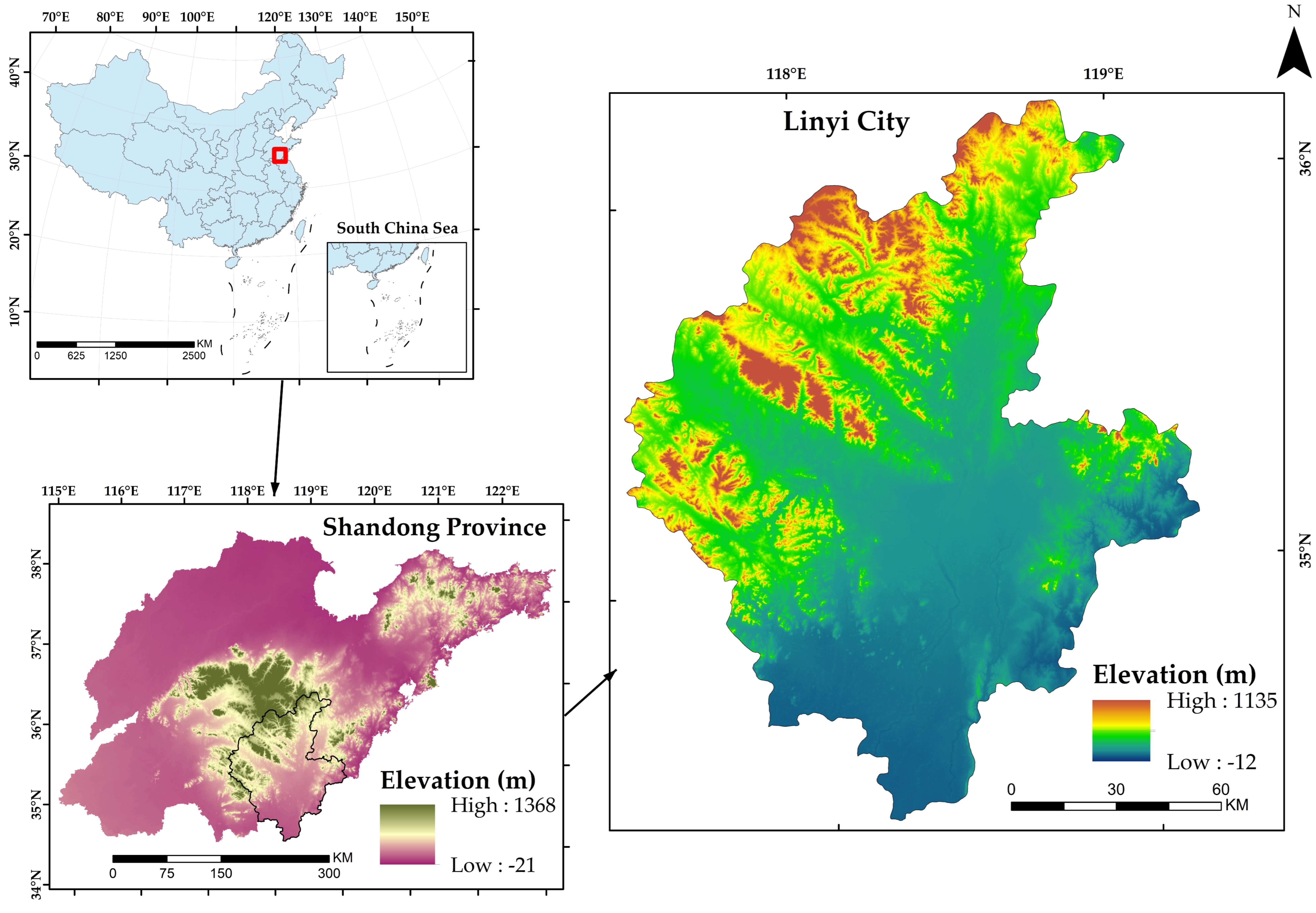
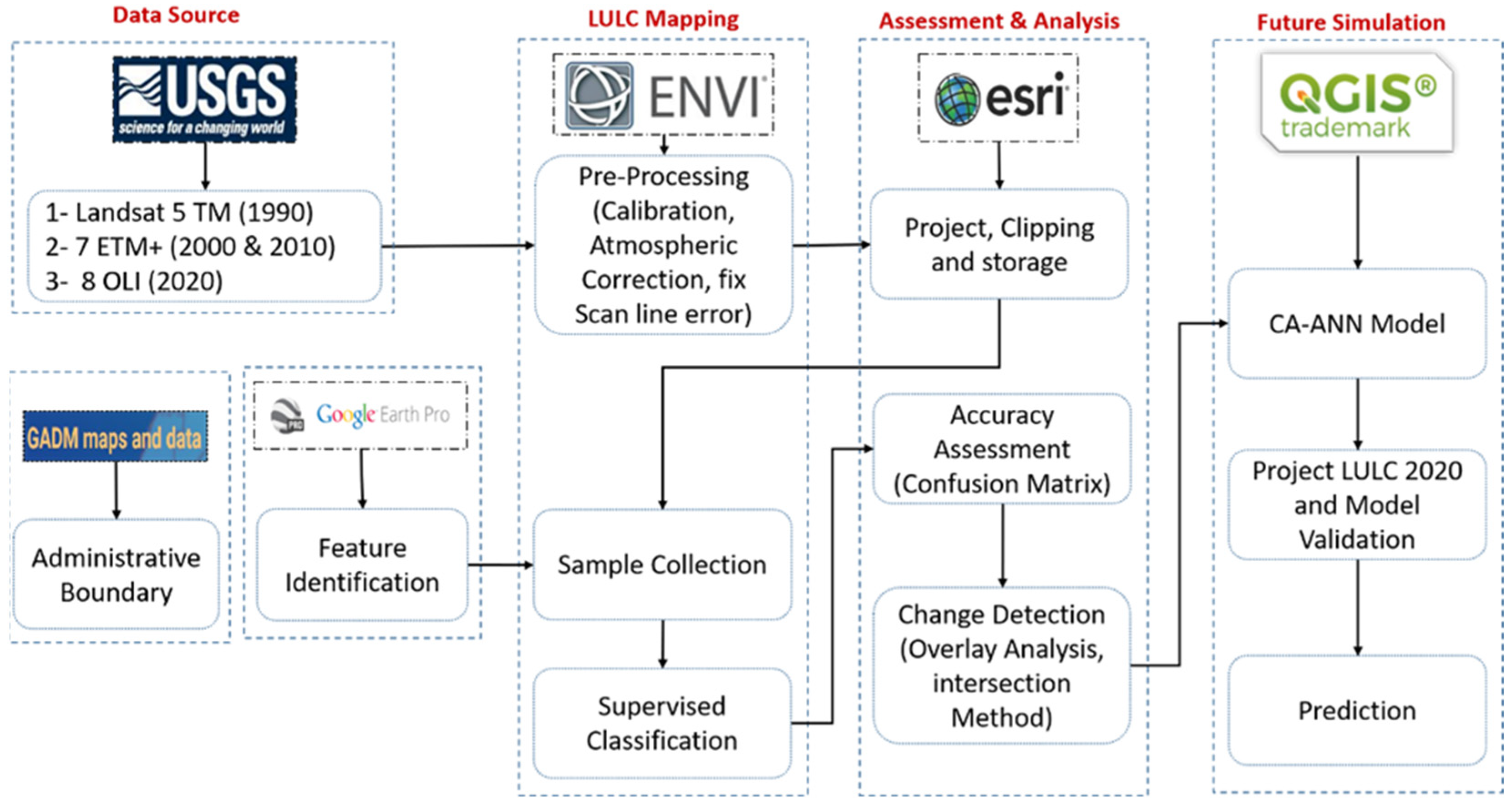
Linyi is among China’s fastest growing cities and has developed into the industrial and technological heart of Shandong province [
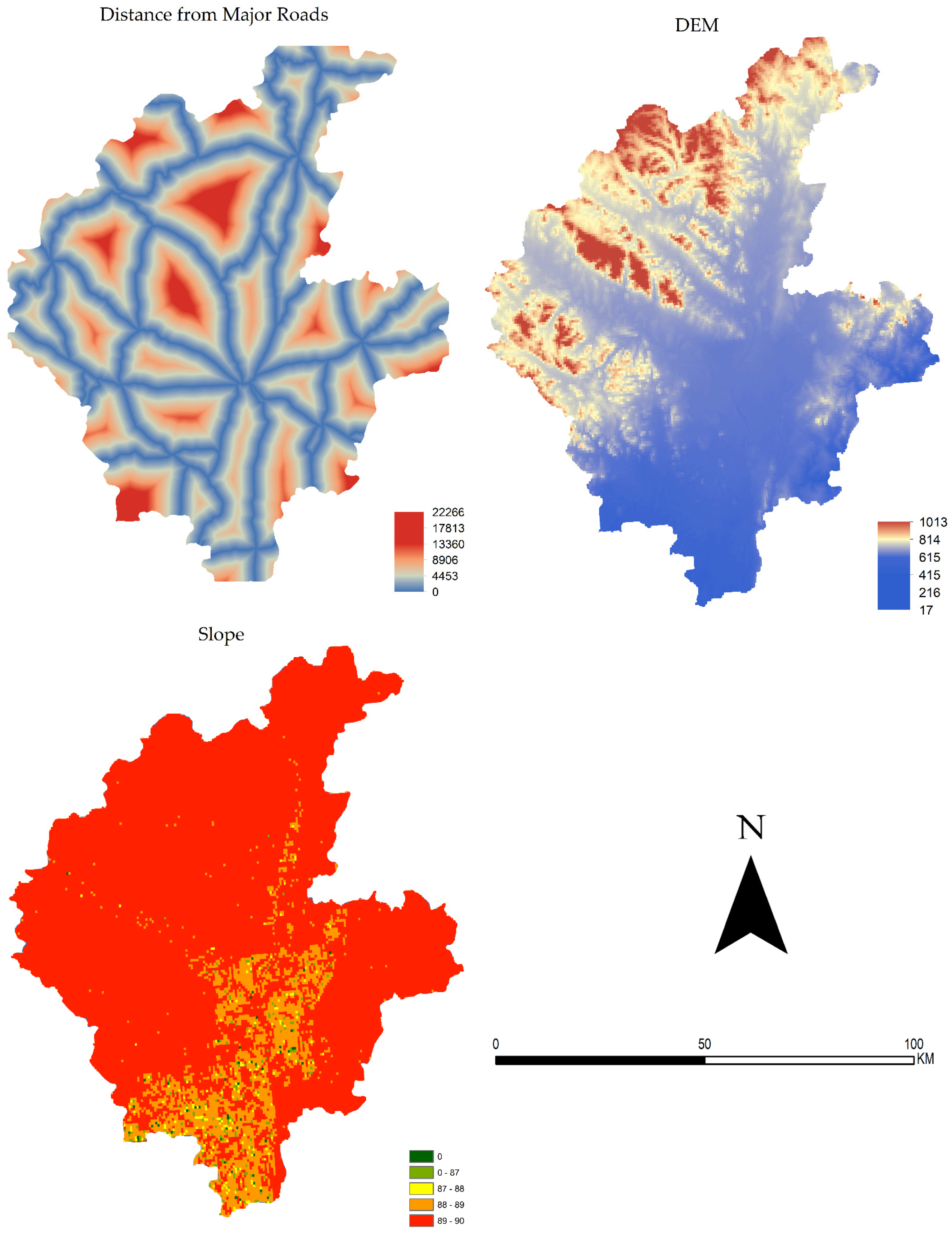
54]. Linyi city underwent a metamorphosis as a result of the recent regional socioeconomic and urban development, having a profound effect on the spatial structure of LULC alterations. We modeled the spatiotemporal transitioning prospects and future scenario of LULC in this work using the Modules for Land-Use Change Simulation (MOLUSCE) plugin underneath QGIS [55,56]. The MOLUSCE plugin is an open-source model for QGIS 2.0 and above, developed by Asia Air Survey to analyze, model, and simulate land use/cover changes (Asia Air Survey). The plugin incorporates a number of well-known algorithms, such as utility modules, cross tabulation techniques, and algorithmic modules, e.g., artificial neural networks (ANNs), multi-criteria evaluation (MCE), weights of evidence (WoE), logistic regression (LR), and Monte Carlo cellular automata (CA) models. To simulate spatiotemporal transitioning possibilities and future LULC predictions for 2030, 2040, and 2050, we used the CA-ANN technique with remotely sensed big data from 1990 to 2020 with a ten-year interval, along with spatial attributes, digital elevation model (DEM), slope, and closeness to roads. After simulating and forecasting the LULC, we supplemented it with indicators to estimate the annual rate of change in LULC classes. Taking all of these factors into consideration, we structured our research with the following specific objectives:
  • Analyzing the degree and change of spatiotemporal LULC trends over the previous four decades by modeling.
  • Forecasting future LULC using socioeconomic and environmental parameters as predictors.
  • Determining the magnitude of LULC change and its possible effects on the geographical pattern.
  • Determining the future LULC intensity scenario.

2. Materials and Methods

2.1. Study Area

Linyi is the biggest prefecture-level city in Shandong Province, China, stretching from 34°22′–36°13′ N and 117°24′–119°11′ E in the country’s southern region, near to the Yellow Sea (Figure 1), with a total area of 17,191.2 square kilometers [57]. The rate of urbanization is 52.75%. The Yi and Shu Rivers create the central axis of the terrain, which is flanked by Meng Shan Mountain to the west and other small ridges to the north and east, producing a fan-shaped alluvial plain to the south. Mountains, hills, and plains have an area ratio of 1:2:2. As of 2011, it is the province’s largest city, both in terms of land area and population [58]. According to the 2020 census, the population was 11,018,365, with an urban population of 3,651,868. Linyi city administers twelve county divisions, consisting of three districts and nine counties. Moreover, Linyi’s economy is based on wholesale marketplaces and is China’s third largest wholesale market, with an annual trading volume of 40 billion RMB (US$5 billion) [59]. In the Linyi prefecture, over 1500 specialized villages and almost 800 industrialized agriculture firms have been established. In 2014, the prefecture’s GDP was 369 billion RMB [60].

2.2. Data Collection

The administrative boundaries were downloaded from GADM. The LULC data for Linyi city were acquired from the Chinese Academy of Sciences’ Resources and Environment Science Data Center (RESDC) between 1990 and 2020 [61]. China’s remotely sensed land use monitoring database is a multi-temporal satellite land use database that spans the entire country. The data are obtained from temporal Landsat (MSS/TM/ETM+/OLI) images that have been artificially interpreted. Six major and twenty-three secondary land-use classes are included in the data, including arable land, wooded land, grassland, water, residential, and barren land, with a spatial resolution of 30 m. They use random sample methods, GPS field surveys, and kappa coefficient testing to ensure the LULC categorization remains accurate. Socioeconomic data are derived using statistics for national sub-counties and the multifactor weight distribution approach. The digital elevation model (DEM) was obtained from WorldClim with a spatial resolution of 30 m and was derived from SRTM elevation data [62]; the slope was estimated using the DEM, and proximity factors such as distance to roads were estimated using the Euclidean distance method in ArcGIS 10.4 (Table 1). The study area was trimmed and projected to WGS 1984 UTM Zone 49N following data collection. Figure 2 depicts the study’s methodological framework.

2.3. Collection of Spatial Variables

Researchers focus on the physical and socioeconomic elements that cause LULC alterations since their impact to the LULC change mechanism is greater. Landsat 5 TM (1990), Landsat 7 ETM+ (2000 & 2010), and Landsat 8 OLI (2020) images, path/row 121/35 and 121/36, and cloud coverage less than 10% were used, which were downloaded from the USGS official website. Physical variables such as geography and climate are seen to be the most significant in encouraging human behavior. Proximity to roadways aids in determining the driving forces behind the landscape design. We employed a variety of physical and proximity considerations (Table 1).
The MOLUSCE plugin provides various well-known methods for evaluating the correlation between LULC data and geographical variables, such as Pearson’s correlation and Cramer’s coefficient. Cramer’s V is a numerical measure of association that varies from 0 to 1, with 1 representing a ‘perfect relationship’ between LULC and the spatial driver and 0 representing ‘no association’. The numbers are not final, and they can only assist in choosing whether to include transition potential modeling or not, although a value greater than 0.1 is often deemed beneficial.

2.4. LULC Classification

After extraction and projection of the study area, we grouped the subtypes of land-use data to obtain five categories: urban land, rural settlements, and other construction land as built-up area; woodland and shrubs as forest; paddy fields, dry land, and cultivated land as cropland; pasture, parks, and green spaces as grassland; and rivers, lakes, reservoirs, and canals as water (Table 2), using the reclassifying tool in ArcGIS 10.4. Then, Google Earth high-resolution images from 2000 were used to interpret and verify the LULC categories. To use the data for transition potential modeling and prediction, we used resampling techniques in ArcGIS to fix the spatial resolution differences between the LULC data and spatial variables.

2.5. Change Analysis and Transition Potential Modeling

We utilized the Modules for Land-Use Change Simulation (MOLUSCE) plugin inside QGIS to estimate spatiotemporal changes and compute the LULC transition between the research intervals (1990–2000, 2000–2010, and 2010–2020), and generated three LULC change maps. We created an area change and transition probability matrix using the LULC data and contextual factors, which included rows and columns of landscape categories in the start and end years. For transition potential modeling, we used the ANN multilayer perceptron approach. As explanatory factors, the DEM, slope, and distance from highways were used (Table 1). These variables are often utilized in LULC change analysis because they give reproducible data on the physical and anthropogenic influences on LULC dynamics.

2.6. Prediction and Model Validation

Simulated models are used to reduce the dynamics of composite urban structures and make them intelligible in a simple manner. We used the CA-ANN technique inside the MOLUSCE plugin to model transition potentials and simulate the future, as many scholars feel the CA-ANN approach is more effective than linear regression [63]. The MOLUSCE plugin efficiently computes land use change analyses [64] and is well-suited for assessing spatiotemporal forest and land-use changes, predicting transition prospects, and simulating future scenarios.
Based on the LULC data for 2000, 2010, explanatory variables, and transition matrices, we projected the LULC for 2020. To validate the model and prediction accuracy, the MOLUSCE plugin offers a kappa validation technique and comparison of actual and projected LULC images. In the ANN learning process, 100 iterations and a neighborhood value of 3 × 3 pixels, a learning rate of 0.001, 12 hidden layers, and 0.05 of momentum were chosen to project the LULC for 2020. After obtaining satisfactory results from the model validation, we employed LULC data from 2010 and 2020 to forecast the LULC in 2030, and the LULC of 2000 and 2020 for 2040. The predicted data for 2030 and 2040 were used to forecast LULC for 2050 (Figure 2).

2.7. Annual Rate of Change Analysis

To obtain the annual rate of change for each land use type, the difference between the final year to initial year, which represents magnitude of change between corresponding years, was divided by the initial year and time period. We used Equation (1) to assess the spatiotemporal magnitude and rate of change in LULC categories:
A R C   ( % ) = F y I y I y × t × 100
where ARC is the annual rate of change in LULC categories. Iy and Fy are the initial and final year areas, respectively, and t is the time interval.

3. Results

3.1. Spatiotemporal Change Analysis

The LULC maps, area statistics, and annual rate of change are shown in Figure 3 and Table 3. During the study period, we observed an uneven shift in land use due to rapid urban expansion (Figure 4), especially a continuous increase in impervious surface from 1815.98 km2 to 4612.60 km2, with an annual increase rate of 5.13%. There was a linear decrease in forest from 2183.52 km2 to 1498.62 km2, with an annual decrease rate of −1.05%. Similarly, green area decreased from 4563.49 km2 to 2841.12 km2, with an annual decrease rate of −1.26%, and barren land from 8538.31 km2 to 7905.13 km2, with an annual decrease rate of −0.25%. In contrast, water faced a linear increase from 224.84 km2 to 286.19 km2, with an annual increase rate of 0.91%. Forest decreased (12.06–4.62%) during 1990–2000 and increased (4.62–8.74%) during 2000–2020. Green area increased (26.34–30.92%) during 1990–2000 and decreased (30.92–16.57%) during 2000–2020. However, impervious surface faced a continuous increasing phenomenon (10.48–26.91%) during the whole study period (1990–2020). Additionally, water decreased (1.30–0.76%) during 1990–2000, increased (0.76–1.97%) during 2000–2010, and decreased (1.97–1.67%) during 2010–2020.
The LULC change analysis explores the spatial dynamic variations in the LULC pattern during the study period. The results from 1990 to 2020 show a notable expansion in impervious surface and a shrinking phenomenon in the forest, green area, and barren land. Figure 5 and Table 4 show the spatiotemporal area and percentage change in all LULC categories. Forest, green area, water, and barren land contributed 5.72%, 21.24%, 0.44%, and 19.45% to the impervious surface, respectively. Figure 6 and Table 5 represent the inter-transition and contribution of LULC categories to changing phenomena from 1990 to 2020. Green area was the largest contributor to the change from 1990–2020, with 21.24% to impervious surface and 9.61% to barren land, while barren land contributed 19.45% to impervious surface, 9.04% to forest, and 5.50% to green area during 1990–2020. However, the contribution of water is very small for the change.

3.2. LULC Transition Analysis

The transition matrix plays an essential role in analyzing temporal changes within a set of LULC categories. The matrix represents the proportions of pixels changing from one land use category to another. The rows of the matrix table represent the categories in the initial year, while the columns show the same order of LULC categories in the final year. The diagonal entries show the size of class stability, and each off-diagonal entry represents the size of the transition from one class to different classes. Values close to 1 in diagonal entries represent the stability of a category. Researchers mostly use transition matrices to compare the temporal changes in different regions [65]. To show how each LULC type was projected to change in our study area, we calculated the transition potential matrix with the help of the MOLUSCE plugin during the periods 1990–2000, 2000–2010, and 2010–2020 based on the existing LULC conditions and explanatory variables.
Table 6 shows the transition potential matrix during 1990–2000, in which barren land and green area were the most stable categories with probabilities of 0.765 and 0.763, respectively, and contributed 0.095 and 0.124 to impervious surface, while water and forest decreased with transition probabilities of 0.642 and 0.204, respectively, and contributed 0.093 and 0.094, respectively, to built-up land. During 2000–2010 (Table 7), the transition values of impervious surface and forest were 0.437 and 0.572, respectively, those of green area and barren land were 0.544 and 0.790, respectively, and that of water was 0.898. Green area and barren land contributed 0.121 and 0.082 to the impervious surface, respectively. Accordingly, during 2010–2020 (Table 8), the transition values of impervious surface and forest were 0.732 and 0.512, respectively, those of green area and barren land were 0.568 and 0.692, respectively, and that of water was 0.657. Green area, barren land, and water contributed 0.279, 0.182, and 0.175 to the impervious surface, respectively. Here, forest contributed 0.094 of the transition to impervious surface. During the study period, only water and forest were stable because of the conservation, afforestation, and reforestation policy of the Chinese government, but significant pressure was on green area and barren land, which donated the largest share to other LULC categories.
Moreover, as we used LULC data from 2000–2020 along with spatial factors for the prediction of 2050 and the transition probability matrix, the transition matrix between 2000 and 2020 (Table 9) showed that water was still stable with a value of 0.816, while forest, green area, barren land, and impervious surface had fragmentation values of 0.598, 0.405, 0.693 and 0.595, respectively. During 2020–2030, forest, green area, and barren land will still experience a decreasing phenomenon (Table 10), while water shows comparatively stable behavior. During 2030–2040, forest and barren land will still experience a decreasing phenomenon (Table 11), while other classes will show comparatively stable behavior. Table 12 represents the transition probability matrix during 2040–2050. Here, we observed that forest and water were the most stable categories, while cropland will experience rapid fragmentation. Table 13 and Figure 7 elaborate the gained and lost areas of each category over each time interval.

3.3. Selection of Spatial Variables

According to transition matrix analysis, we observed that the significant growth in impervious surface was mainly due to green area and barren land fragmentation. All these transitions were based on physical and socioeconomic driving factors. Researchers mostly use these spatial factors to investigate LULC dynamics.
Table 14 shows the prospective Cramer’s V value of each spatial variable. The Cramer’s V value suggests that the variables are ideal for transition potential modeling, as their values are more significant. According to the values, the selection of physical and socioeconomic explanatory variables is more effectual, i.e., DEM: 0.37; slope: 0.22; and distance from road: 0.09. Figure 8 shows the spatial variables used in this study.

3.4. Transition Potential Modeling and Model Validation

The MOLUSCE plugin integrates some well-known algorithms for transition potential modeling, such as the ANN (multilayer perceptron), weights of evidence, multicriteria evaluation, logistic regression, and CA algorithm, for future simulation. The spatial variables for model calibration were chosen based on their relatively strong association with LULC, as measured by Cramer’s coefficient.
We used the CA-ANN approach for transition potential modeling and prediction. We employed LULC data from 2000–2010 along with spatial variables to project LULC for 2020 and obtained a validation kappa value of 0.97. After obtaining the projected LULC, we compared the actual LULC of 2020 with the projected data and obtained an overall accuracy of 65.80% and an overall kappa value of 0.48. Figure 9 and Table 15 show the actual and forecasted maps and statistics for 2020.

3.5. Prediction of LULC

After obtaining satisfactory results from model validation, we predicted the LULC for 2030, 2040, and 2050. We employed the temporal LULC data from 2010 and 2020, the spatial variables, and the transition probability matrix (Table 9) to predict the LULC for 2030 and obtained a kappa value of 0.61. Furthermore, the LULC of 2000 and 2020, including the explanatory variables and transition matrix (Table 10), were used for the prediction of 2040, and we obtained a kappa value of 0.51. Finally, we predicted the LULC for 2050 based on the projected data for 2030–2040 and the transition matrix (Table 11) and obtained a kappa value of 0.51. Figure 10 and Table 16 represent the map, area statistics, and overall validation kappa of the predicted LULC of 2030, 2040, and 2050.

3.6. Prediction of Change

The LULC change analysis explores the spatial dynamic variations in the LULC pattern during the study period. The results from 2020 to 2050 show a notable expansion in impervious surface and a shrinking phenomenon in the green area and barren land. Figure 11 and Table 17 show the spatiotemporal area and percentage change in all LULC categories. Green area and water contributed 5.19 and 1.69 to the impervious surface, respectively. Table 18 represents the inter-transition and contribution of LULC categories to changing phenomena from 2020 to 2050. Green area is the largest contributor to the change from 2020–2050, with 5.19% to impervious surface and 0.56% to barren land, while barren land contributed 1.69% to impervious surface and 3.95% to forest.

4. Discussion

Globally, and particularly in the 21st century, enormous urbanization processes have altered the natural habitat and landscape layout. Urbanization is primarily driven by physical and socioeconomic reasons such as geography, demography, and economic expansion. Socioeconomic development, however, has a higher impact on the urban expansion than overpopulation. The size and speed with which cities are expanding and fragmenting landscape patterns has raised worries about climate change, food security, and natural resource shortages.
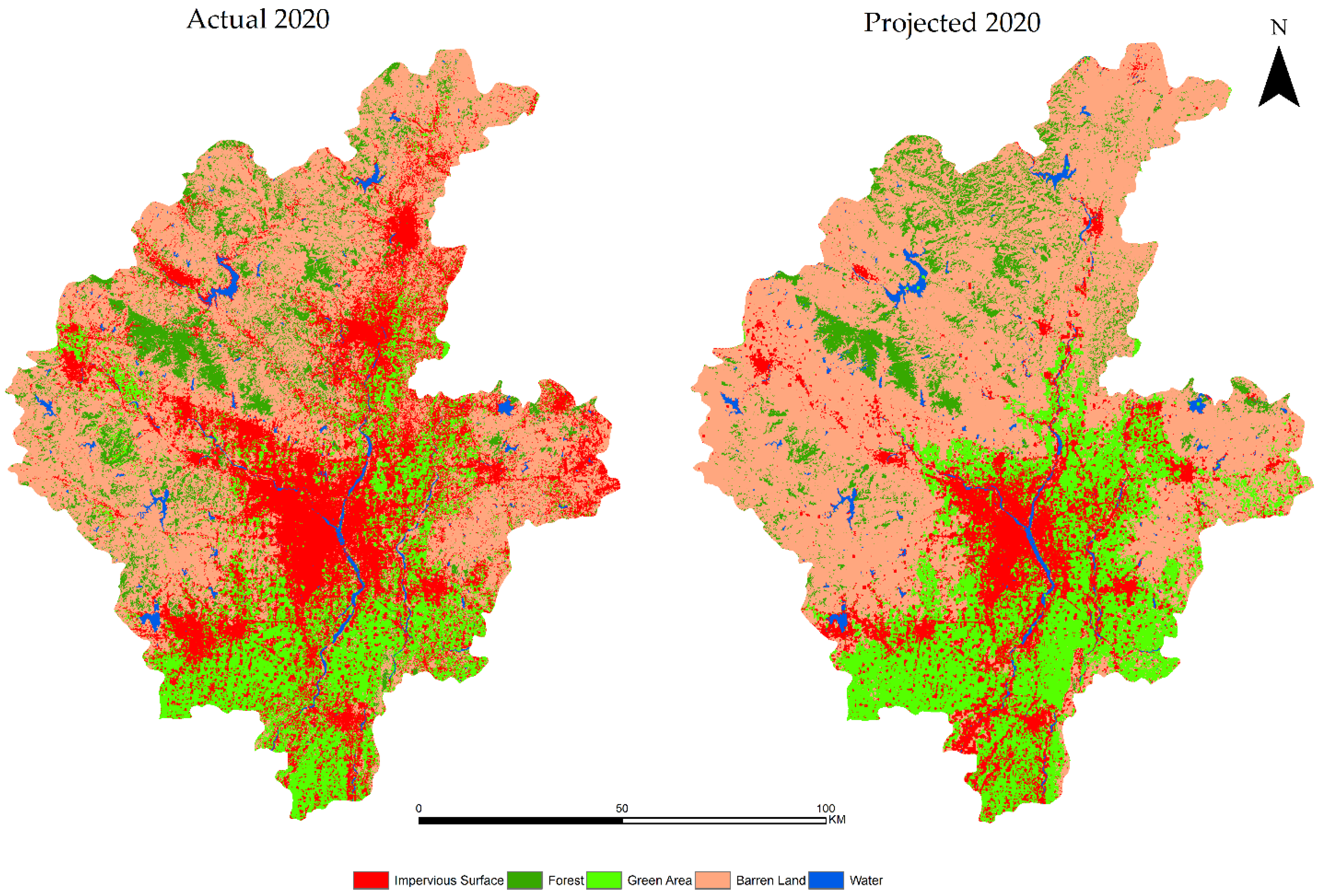
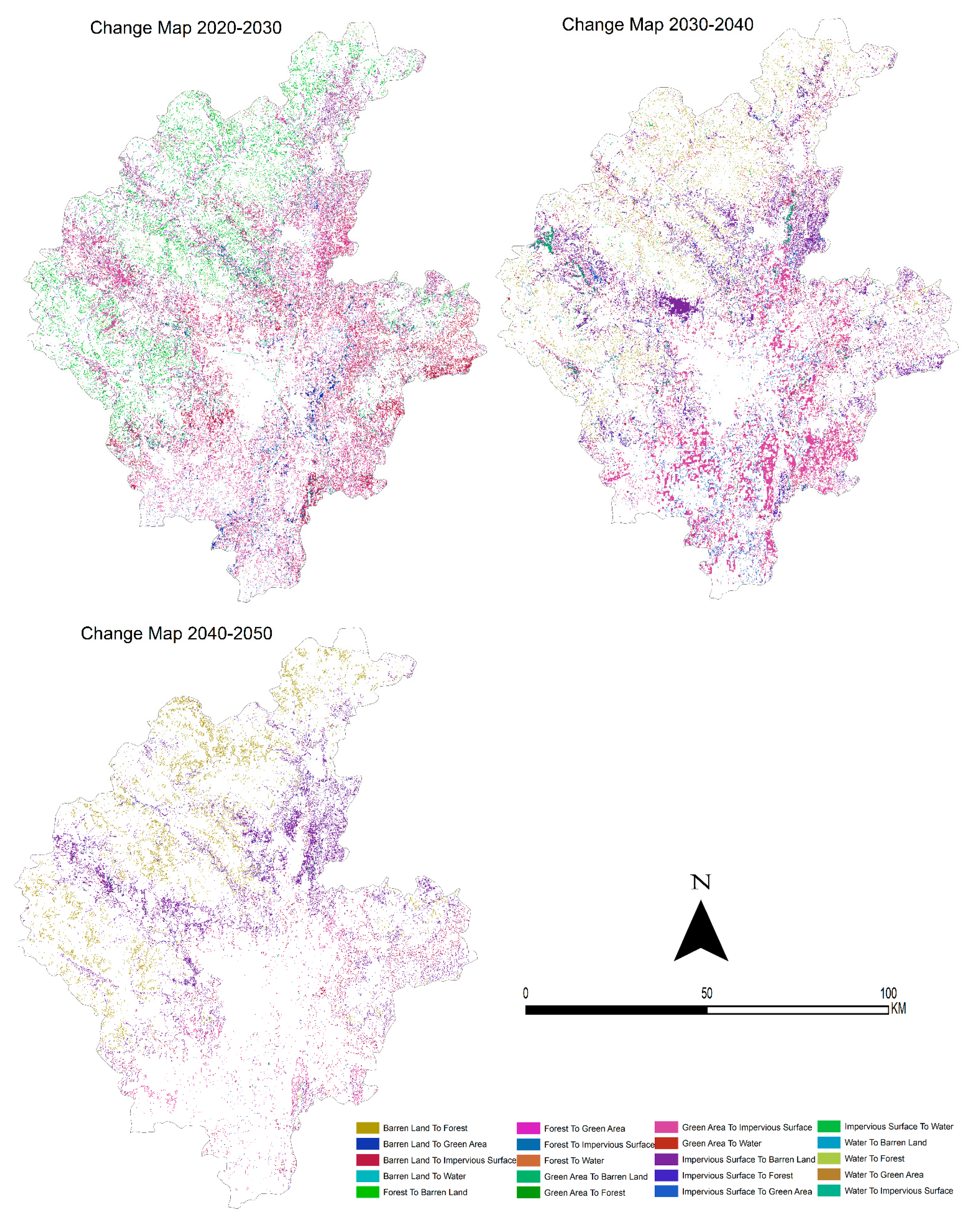
Changes in LULC are inextricably tied to geography and development policies. Following China’s late 1970s ‘opening up’ strategy, economic reforms resulted in huge movement, immigration, and urban expansion. We examined the shift from 1990 to 2020 using spatiotemporal LULC data and physical and socioeconomic driving factors, and produced a transition probability matrix for each interval using the MOLUSCE plugin within QGIS software. Additionally, we predicted the LULC for 2030, 2040, and 2050 using the CA-ANN multilayer perceptron technique included in the MOLUSCE plugin.
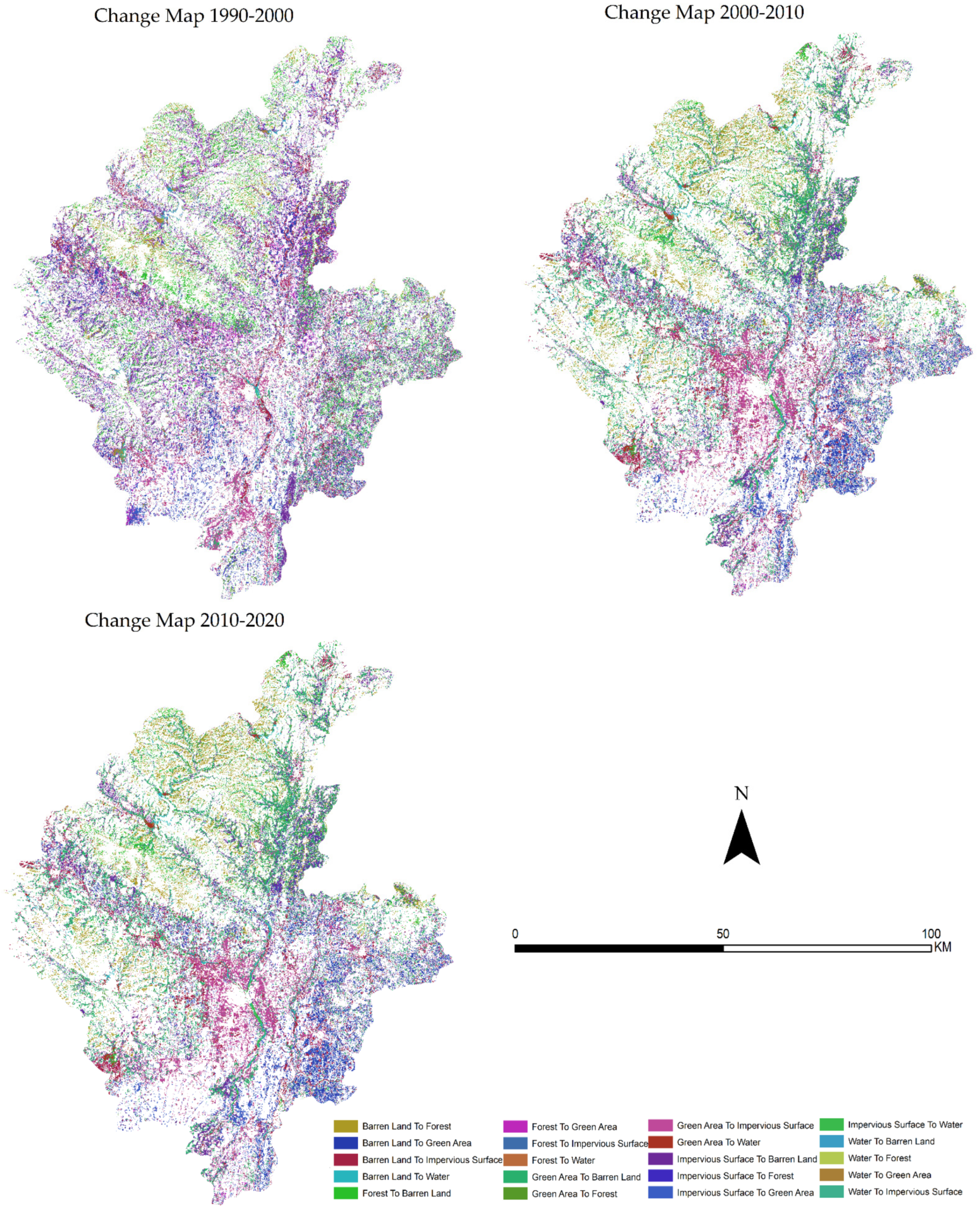
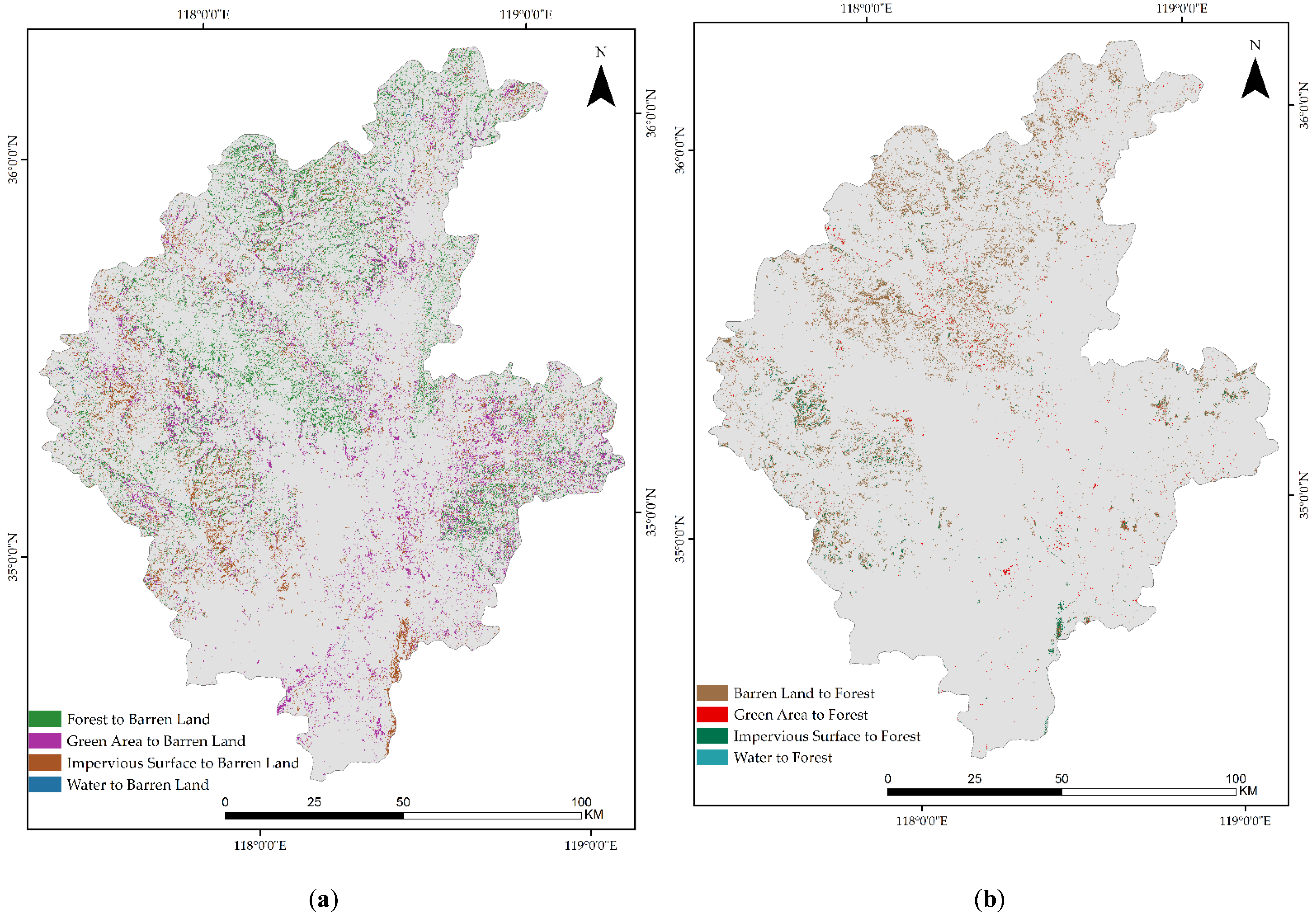
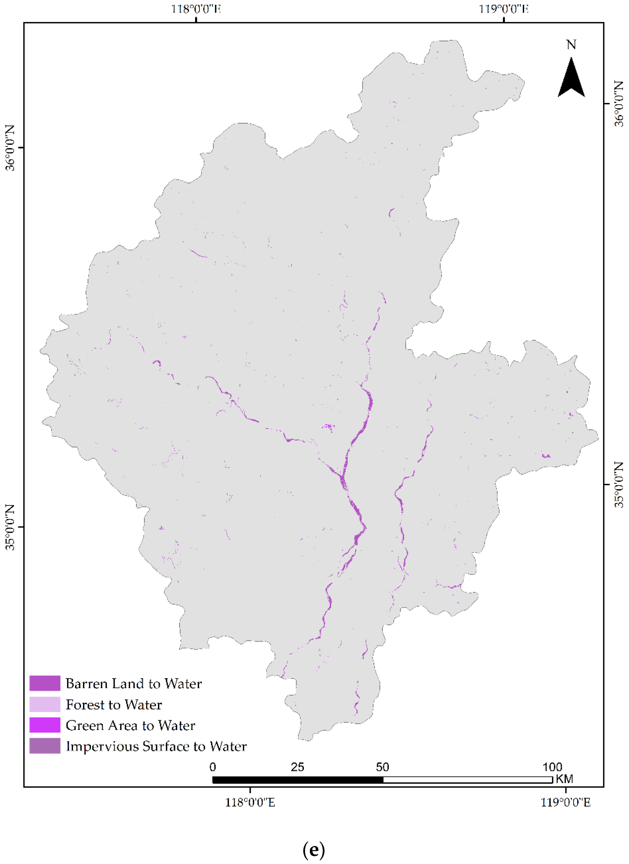
Our findings suggest that during the research period, physical and socioeconomic factors had a substantial impact on landscape patterns. In general, locations with lower elevations have more rapid LULC changes, as their geography is more conducive to human activity. The greatest modifications happened in Linyi’s plain sections, particularly along the Yi River, where the slope is relatively lower than in other parts. The northern, eastern, and western regions, which are mountainous and hilly, do not suffer from rapid fragmentation.
Linyi’s vision of a trade gateway encapsulates broader objectives of market-oriented reforms and cooperation in the socioeconomic sector, education, innovation, international business, and technical advancement. Numerous studies have demonstrated that population increase and economic development are the primary factors driving built-up expansion [66,
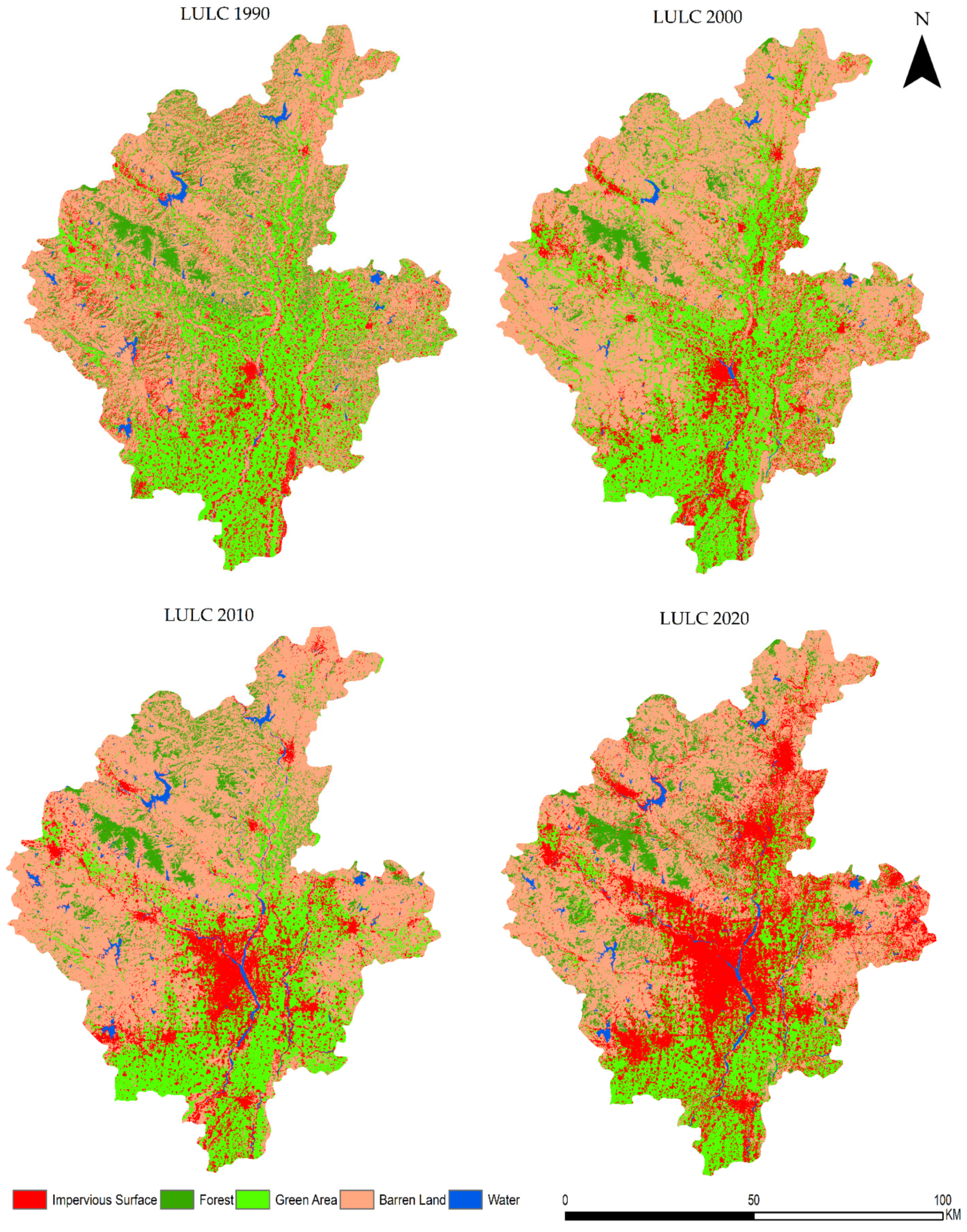
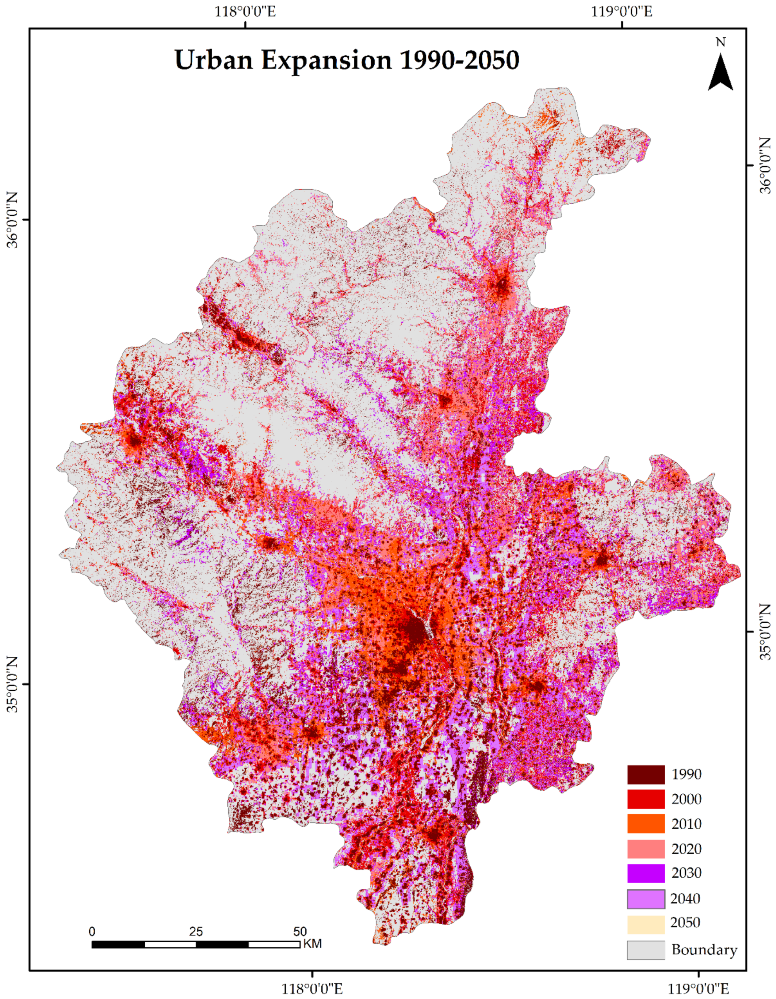
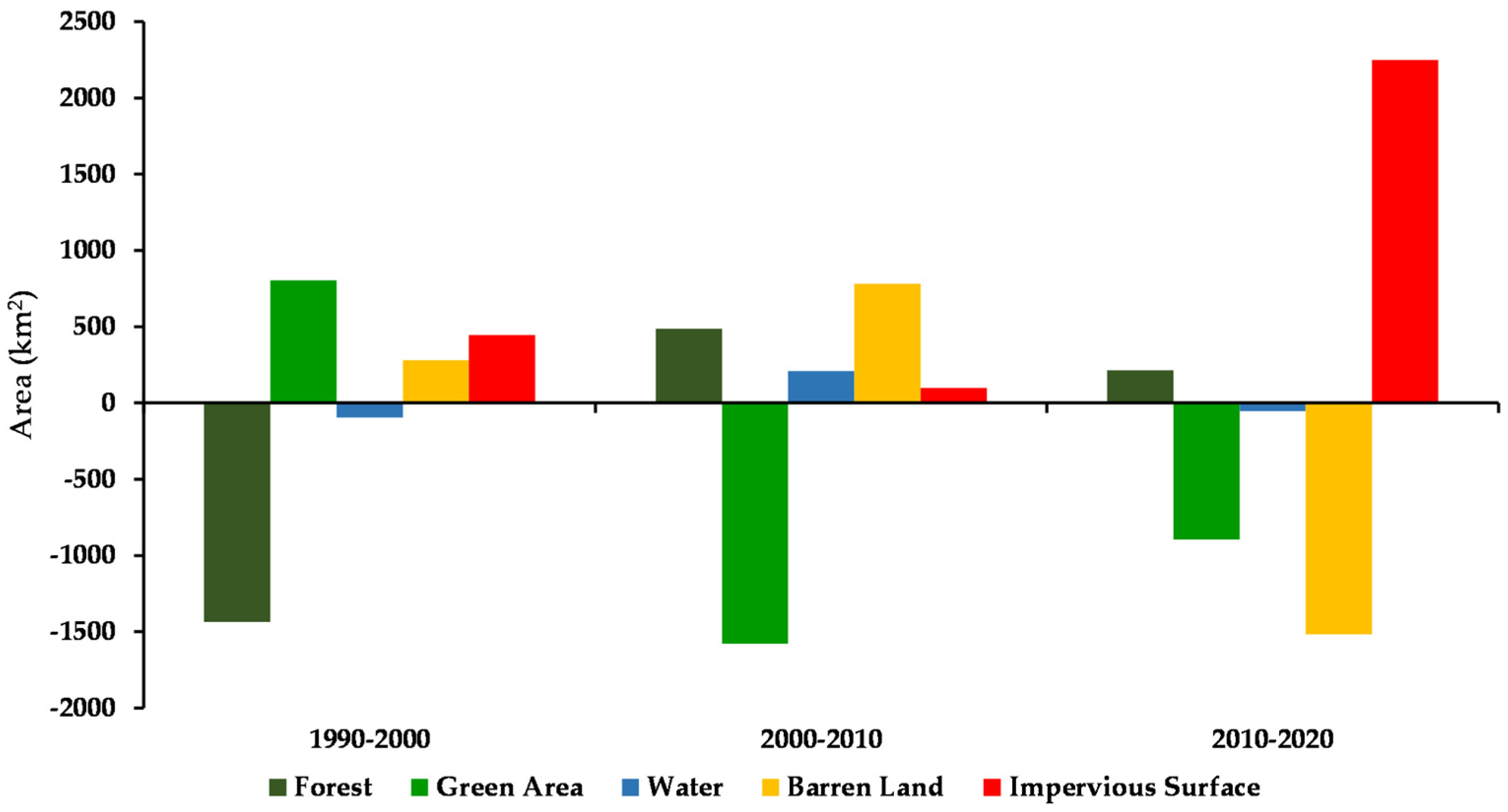
67]. The growing urban area has a detrimental influence on the environment, aquatic habitat, and biodiversity. According to our findings, Linyi’s LULC has undergone a remarkable transformation over the last three decades due to rapid urbanization, most notably in the rapid conversion of green space and barren land to impervious surface during the last decade. From 1990 to 2020, the impervious surface increased from 10.48 to 26.91%, and forest contributed 5.72%, green area contributed 21.24%, barren land contributed 19.45%, and water contributed 0.44%. Additionally, the future simulation results show that impervious surface will continue to increase from 2030 to 2040 with percentages of 34.36% to 34.50%, and decrease from 2040–2050 with percentages of 34.50% to 30.75%. However, the green area will continue to decrease from 2030–2050 with percentages of 11.79% to 6.97%.
Ultimately, dramatic changes in LULC, particularly urban growth and fragmentation of green space, could jeopardize natural resources, the environment, and food security. Thus, the spatiotemporal and prospective LULC simulation results will aid policymakers in analyzing the change in LULC intensity and the socioeconomic elements that influence it, as well as in promoting environmental conservation and sustainable development policies. Additionally, we modeled and predicted LULC using solely physical and socioeconomic characteristics. However, future research can incorporate development policies and climate variables.

5. Conclusions

In this study, we analyzed spatiotemporal LULC changes based on temporal Landsat data, and projected future scenarios based on driving factors in Linyi city, China. Linyi city faces the challenge of agricultural land, environmental deterioration, and water quality depletion as a result of fast urban growth and fragmentation of forest and green areas. These factors exacerbate the difficulties associated with sustaining regional development and environmental conservation. We modeled and predicted landscape patterns using solely physical and socioeconomic elements in this study, although development policies, migration, immigration, and climatic conditions may all have an effect on landscape patterns. Additionally, agriculture and development policies can be linked to promote sustainable urbanization. It is advised that future studies use more factors and data to investigate their effects on landscape patterns.

Author Contributions

R.M. and W.Z. designed the approaches and proposed the basic idea. R.M. and Z.A. processed the data, performed the analysis, and wrote the manuscript. W.Z. supervised the study. F.G. and L.G. helped to modify the manuscript and provided useful suggestions. All authors have read and agreed to the published version of the manuscript.

Funding

This work was partially funded by the Key Research and Development Program of Shandong Province (2019GNC106027, 2019JZZY010134) and the Natural Science Foundation of Shandong Province (ZR2020MF058, ZR2020MF029).

Institutional Review Board Statement

Not applicable.

Informed Consent Statement

Not applicable.

Data Availability Statement

Data can be obtained on request to the Corresponding Author.

Conflicts of Interest

The authors declare no conflict of interest.

References

  1. Shaw, S.-L.; Tsou, M.-H.; Ye, X. Human dynamics in the mobile and big data era. Int. J. Geogr. Inf. Sci. 2016, 30, 1687–1693. [Google Scholar] [CrossRef]
  2. Zheng, Z.; Wu, Z.; Chen, Y.; Yang, Z.; Marinello, F. Detection of City Integration Processes in Rapidly Urbanizing Areas Based on Remote Sensing Imagery. Land 2020, 9, 378. [Google Scholar] [CrossRef]
  3. Chi, M.; Plaza, A.; Benediktsson, J.A.; Sun, Z.; Shen, J.; Zhu, Y. Big Data for Remote Sensing: Challenges and Opportunities. Proc. IEEE 2016, 104, 2207–2219. [Google Scholar] [CrossRef]
  4. Dey, N.; Bhatt, C.; Ashour, A.S. Big Data for Remote Sensing: Visualization, Analysis and Interpretation; Springer: Cham, Switzerland, 2018; p. 104. [Google Scholar]
  5. Sedona, R.; Cavallaro, G.; Jitsev, J.; Strube, A.; Riedel, M.; Benediktsson, J.A. Remote Sensing Big Data Classification with High Performance Distributed Deep Learning. Remote Sens. 2019, 11, 3056. [Google Scholar] [CrossRef] [Green Version]
  6. Li, S.; Dragicevic, S.; Anton, F.; Sester, M.; Winter, S.; Çöltekin, A.; Pettit, C.; Jiang, B.; Haworth, J.; Stein, A.; et al. Geospatial big data handling theory and methods: A review and research challenges. ISPRS J. Photogramm. Remote Sens. 2016, 115, 119–133. [Google Scholar] [CrossRef] [Green Version]
  7. Jiang, Z.; Shekhar, S. Spatial Big Data Science; Springer International Publishing AG: Cham, Switzerland, 2017. [Google Scholar]
  8. Roy, D.P.; Wulder, M.A.; Loveland, T.R.; Woodcock, C.E.; Allen, R.G.; Anderson, M.C.; Helder, D.; Irons, J.R.; Johnson, D.M.; Kennedy, R.; et al. Landsat-8: Science and product vision for terrestrial global change research. Remote Sens. Environ. 2014, 145, 154–172. [Google Scholar] [CrossRef] [Green Version]
  9. Agarwal, C.; Green, G.M.; Grove, J.M.; Evans, T.P.; Schweik, C.M. A Review and Assessment of Land-Use Change Models: Dynamics of Space, Time, and Human Choice; General Technical Report; U.S. Department of Agriculture, Forest Service, Northeastern Research Station: Newton Square, PA, USA, 2002. [Google Scholar]
  10. Halefom, A.; Teshome, A.; Sisay, E.; Ahmad, I. Dynamics of Land Use and Land Cover Change Using Remote Sensing and GIS: A Case Study of Debre Tabor Town, South Gondar, Ethiopia. J. Geogr. Inf. Syst. 2018, 10, 165–174. [Google Scholar] [CrossRef] [Green Version]
  11. Mondal, M.S.; Sharma, N.; Garg, P.K.; Kappas, M. Statistical independence test and validation of CA Markov land use land cover (LULC) prediction results. Egypt. J. Remote Sens. Space Sci. 2016, 19, 259–272. [Google Scholar] [CrossRef] [Green Version]
  12. Tasser, E.; Leitinger, G.; Tappeiner, U. Climate change versus land-use change—What affects the mountain landscapes more? Land Use Policy 2017, 60, 60–72. [Google Scholar] [CrossRef]
  13. Bhunia, G.S.; Chatterjee, U.; Shit, P.K. Emergence and challenges of land reclamation: Issues and prospect. Mod. Cartogr. Ser. 2021, 10, 1–15. [Google Scholar] [CrossRef]
  14. Pribadi, D.O.; Pauleit, S. The dynamics of peri-urban agriculture during rapid urbanization of Jabodetabek Metropolitan Area. Land Use Policy 2015, 48, 13–24. [Google Scholar] [CrossRef]
  15. Slonecker, E.T.; Jennings, D.B.; Garofalo, D. Remote sensing of impervious surfaces: A review. Remote Sens. Rev. 2001, 20, 227–255. [Google Scholar] [CrossRef]
  16. Wongsai, N.; Wongsai, S.; Lim, A.; McNeil, D.; Huete, A.R. Impacts of spatial heterogeneity patterns on long-term trends of Moderate Resolution Imaging Spectroradiometer (MODIS) land surface temperature time series. J. Appl. Remote Sens. 2020, 14, 014513. [Google Scholar] [CrossRef]
  17. Iqbal, M.F.; Khan, I.A. Spatiotemporal land use land cover change analysis and erosion risk mapping of Azad Jammu and Kashmir, Pakistan. Egypt. J. Remote Sens. Space Sci. 2014, 17, 209–229. [Google Scholar]
  18. Journals, I.; Al Mamun, A.; Mahmood, A.; Rahman, M. Identification and Monitoring the Change of Land Use Pattern Using Remote Sensing and GIS: A Case Study of Dhaka City. OSR J. Mech. Civ. Eng. 2013, 6, 20–28. [Google Scholar] [CrossRef]
  19. Gao, J.; Liu, Y. Determination of land degradation causes in Tongyu County, Northeast China via land cover change detection. Int. J. Appl. Earth Obs. Geoinf. 2010, 12, 9–16. [Google Scholar] [CrossRef]
  20. Huang, K.; Li, X.; Liu, X.; Seto, K.C. Projecting global urban land expansion and heat island intensification through 2050. Environ. Res. Lett. 2019, 14, 114037. [Google Scholar] [CrossRef] [Green Version]
  21. Leeson, G.W. The Growth, Ageing and Urbanisation of our World. J. Popul. Ageing 2018, 11, 107–115. [Google Scholar] [CrossRef] [Green Version]
  22. Lang, W.; Long, Y.; Chen, T. Rediscovering Chinese cities through the lens of land-use patterns. Land Use Policy 2018, 79, 362–374. [Google Scholar] [CrossRef]
  23. Gu, C. Urbanization: Processes and driving forces. Sci. China Earth Sci. 2019, 62, 1351–1360. [Google Scholar] [CrossRef]
  24. Vanbergen, A.J.; Aizen, M.A.; Cordeau, S.; Garibaldi, L.A.; Garratt, M.P.; Kovács-Hostyánszki, A.; Lecuyer, L.; Ngo, H.T.; Potts, S.G.; Settele, J.; et al. Transformation of agricultural landscapes in the Anthropocene: Nature’s contributions to people, agriculture and food security. Adv. Ecol. Res. 2020, 63, 193–253. [Google Scholar] [CrossRef]
  25. Abbas, Z.; Yang, G.; Zhong, Y.; Zhao, Y. Spatiotemporal Change Analysis and Future Scenario of LULC Using the CA-ANN Approach: A Case Study of the Greater Bay Area, China. Land 2021, 10, 584. [Google Scholar] [CrossRef]
  26. Yue, W.; Fan, P.; Wei, Y.D.; Qi, J. Economic development, urban expansion, and sustainable development in Shanghai. Stoch. Hydrol. Hydraul. 2012, 28, 783–799. [Google Scholar] [CrossRef]
  27. Wu, Y.; Luo, J.; Zhang, X.; Skitmore, M. Urban growth dilemmas and solutions in China: Looking forward to 2030. Habitat Int. 2016, 56, 42–51. [Google Scholar] [CrossRef] [Green Version]
  28. Wei, Y.D.; Ye, X. Urbanization, urban land expansion and environmental change in China. Stoch. Hydrol. Hydraul. 2014, 28, 757–765. [Google Scholar] [CrossRef]
  29. Liu, J.; Coomes, D.A.; Gibson, L.; Hu, G.; Liu, J.; Luo, Y.; Wu, C.; Yu, M. Forest fragmentation in China and its effect on biodiversity. Biol. Rev. 2019, 94, 1636–1657. [Google Scholar] [CrossRef]
  30. Tao, W.; Liu, J.; Ban-Weiss, G.A.; Zhang, L.; Zhang, J.; Yi, K.; Tao, S. Potential impacts of urban land expansion on Asian airborne pollutant outflows. J. Geophys. Res. Atmos. 2017, 122, 7646–7663. [Google Scholar] [CrossRef]
  31. Jacobson, M.Z.; Nghiem, S.V.; Sorichetta, A.; Whitney, N. Ring of impact from the mega-urbanization of Beijing between 2000 and 2009. J. Geophys. Res. Atmos. 2015, 120, 5740–5756. [Google Scholar] [CrossRef]
  32. Mahmoud, S.H.; Gan, T.Y. Impact of anthropogenic climate change and human activities on environment and ecosystem services in arid regions. Sci. Total Environ. 2018, 633, 1329–1344. [Google Scholar] [CrossRef]
  33. Puplampu, D.A.; Boafo, Y.A. Exploring the impacts of urban expansion on green spaces availability and delivery of ecosystem services in the Accra metropolis. Environ. Chall. 2021, 5, 100283. [Google Scholar] [CrossRef]
  34. Vasenev, V.; Stoorvogel, J.; Leemans, R.; Valentini, R.; Hajiaghayeva, R. Projection of urban expansion and related changes in soil carbon stocks in the Moscow Region. J. Clean. Prod. 2018, 170, 902–914. [Google Scholar] [CrossRef]
  35. Ometto, J.P.; Sousa-Neto, E.R.; Tejada, G. Land Use, Land Cover and Land Use Change in the Brazilian Amazon (1960–2013). In Interactions between Biosphere, Atmosphere and Human Land Use in the Amazon Basin; Springer: Berlin/Heidelberg, Germany, 2016; pp. 369–383. [Google Scholar]
  36. Adhikari, A.; Hansen, A.J. Land use change and habitat fragmentation of wildland ecosystems of the North Central United States. Landsc. Urban Plan. 2018, 177, 196–216. [Google Scholar] [CrossRef]
  37. Wolff, N.H.; Masuda, Y.J.; Meijaard, E.; Wells, J.; Game, E. Impacts of tropical deforestation on local temperature and human well-being perceptions. Glob. Environ. Chang. 2018, 52, 181–189. [Google Scholar] [CrossRef]
  38. Hatab, A.A.; Cavinato, M.E.R.; Lindemer, A.; Lagerkvist, C.J. Urban sprawl, food security and agricultural systems in developing countries: A systematic review of the literature. Cities 2019, 94, 129–142. [Google Scholar] [CrossRef]
  39. Akın, A.; Sunar, F.; Berberoglu, S. Urban change analysis and future growth of Istanbul. Environ. Monit. Assess. 2015, 187, 1–15. [Google Scholar] [CrossRef]
  40. Soares-Filho, B.S.; Cerqueira, G.C.; Pennachin, C.L. dinamica—a stochastic cellular automata model designed to simulate the landscape dynamics in an Amazonian colonization frontier. Ecol. Model. 2002, 154, 217–235. [Google Scholar] [CrossRef]
  41. Chen, Z.; Huang, M.; Zhu, D.; Altan, O. Integrating Remote Sensing and a Markov-FLUS Model to Simulate Future Land Use Changes in Hokkaido, Japan. Remote Sens. 2021, 13, 2621. [Google Scholar] [CrossRef]
  42. Liu, X.; Sun, R.; Yang, Q.; Su, G.; Qi, W. Simulating urban expansion using an improved SLEUTH model. J. Appl. Remote Sens. 2012, 6, 061709. [Google Scholar] [CrossRef] [Green Version]
  43. Pahlavani, P.; Omran, H.A.; Bigdeli, B. A multiple land use change model based on artificial neural network, Markov chain, and multi objective land allocation. Earth Obs. Geomat. Eng. 2017, 1, 82–99. [Google Scholar]
  44. Rahman, M.T.U.; Tabassum, F.; Rasheduzzaman, M.; Saba, H.; Sarkar, L.; Ferdous, J.; Uddin, S.Z.; Islam, A.Z.M.Z. Temporal dynamics of land use/land cover change and its prediction using CA-ANN model for southwestern coastal Bangladesh. Environ. Monit. Assess. 2017, 189, 1–18. [Google Scholar] [CrossRef] [PubMed]
  45. Cheng, L.; Sun, H.; Zhang, Y.; Zhen, S. Spatial structure optimization of mountainous abandoned mine land reuse based on system dynamics model and CLUE-S model. Int. J. Coal Sci. Technol. 2019, 6, 113–126. [Google Scholar] [CrossRef] [Green Version]
  46. Pu, R. Mapping Tree Species Using Advanced Remote Sensing Technologies: A State-of-the-Art Review and Perspective. J. Remote Sens. 2021, 2021, 9812624. [Google Scholar] [CrossRef]
  47. Li, X.; Chen, Y.; Liu, X.; Xu, X.; Chen, G. Experiences and issues of using cellular automata for assisting urban and regional planning in China. Int. J. Geogr. Inf. Sci. 2017, 31, 1606–1629. [Google Scholar] [CrossRef]
  48. Ngie, A.; Abutaleb, K.; Ahmed, F.; Taiwo, O.-J. Spatial modelling of urban change using satellite remote sensing: A review. Life Chang. Urban Landsc. 2013, 1, 3. [Google Scholar] [CrossRef]
  49. Gomes, E.; Banos, A.; Abrantes, P.; Rocha, J.; Schläpfer, M. Future land use changes in a peri-urban context: Local stakeholder views. Sci. Total Environ. 2020, 718, 137381. [Google Scholar] [CrossRef]
  50. Tamiminia, H.; Salehi, B.; Mahdianpari, M.; Quackenbush, L.; Adeli, S.; Brisco, B. Google Earth Engine for geo-big data applications: A meta-analysis and systematic review. ISPRS J. Photogramm. Remote Sens. 2020, 164, 152–170. [Google Scholar] [CrossRef]
  51. Lillesand, T.; Kiefer, R.; Chipman, J. Remote Sensing and Image Interpretation, 6th ed.; John Wiley & Sons: Hoboken, NJ, USA, 2015. [Google Scholar]
  52. Nagendra, H.; Lucas, R.; Honrado, J.P.; Jongman, R.H.; Tarantino, C.; Adamo, M.; Mairota, P. Remote sensing for conservation monitoring: Assessing protected areas, habitat extent, habitat condition, species diversity, and threats. Ecol. Indic. 2013, 33, 45–59. [Google Scholar] [CrossRef]
  53. Halmy, M.W.A.; Gessler, P.E.; Hicke, J.A.; Salem, B. Land use/land cover change detection and prediction in the north-western coastal desert of Egypt using Markov-CA. Appl. Geogr. 2015, 63, 101–112. [Google Scholar] [CrossRef]
  54. Qianyi, W.; Ran, L.; Kee-Cheok, C. Alternative Globalisations and the Role of China’s Secondary Cities: Three Case Studies. China Int. J. 2019, 17, 95–111. [Google Scholar]
  55. Perović, V.; Jakšić, D.; Jaramaz, D.; Koković, N.; Čakmak, D.; Mitrović, M.; Pavlović, P. Spatio-temporal analysis of land use/land cover change and its effects on soil erosion (Case study in the Oplenac wine-producing area, Serbia). Environ. Monit. Assess. 2018, 190, 1–18. [Google Scholar] [CrossRef] [PubMed]
  56. Satya, B.A.; Shashi, M.; Deva, P. Future land use land cover scenario simulation using open source GIS for the city of Warangal, Telangana, India. Appl. Geomatics 2020, 12, 281–290. [Google Scholar] [CrossRef]
  57. Zhong, S.; Zheng, Z.; Liu, Z. The Impact of Government Development Policy on Land Investment and Land Price: Evidences from Linyi. J. Korea Contents Assoc. 2021, 21, 337–347. [Google Scholar]
  58. Xun, F.; Hu, Y. Evaluation of ecological sustainability based on a revised three-dimensional ecological footprint model in Shandong Province, China. Sci. Total Environ. 2019, 649, 582–591. [Google Scholar] [CrossRef]
  59. Zhu, H.; Huang, X.; He, Q.; Li, J.; Ren, L. Sustaining Competitiveness: Moving Towards Upstream Manufacturing in Specialized-Market-Based Clusters in the Chinese Toy Industry. Sustainability 2016, 8, 176. [Google Scholar] [CrossRef] [Green Version]
  60. Schneider, M. Dragon Head Enterprises and the State of Agribusiness in China. J. Agrar. Chang. 2017, 17, 3–21. [Google Scholar] [CrossRef]
  61. Brudvig, L.A.; Damschen, E.I.; Haddad, N.M.; Levey, D.J.; Tewksbury, J.J. The influence of habitat fragmentation on multiple plant-animal interactions and plant reproduction. Ecology 2015, 96, 2669–2678. [Google Scholar] [CrossRef]
  62. WorldClim. Available online: http://www.worldclim.org/ (accessed on 16 July 2020).
  63. El-Tantawi, A.M.; Bao, A.; Chang, C.; Liu, Y. Monitoring and predicting land use/cover changes in the Aksu-Tarim River Basin, Xinjiang-China (1990–2030). Environ. Monit. Assess. 2019, 191, 1–18. [Google Scholar] [CrossRef]
  64. Gismondi, M. MOLUSCE-an Open Source Land Use Change Analyst. 2013. Available online: https://2013.foss4g.org/conf/programme/presentations/107/ (accessed on 17 July 2021).
  65. Xiao, J.; Watanabe, T.; Lu, X.; Chand, M.B.; Umarhadi, D.A.; Chen, X.; Avtar, R. Integrating land use/land cover change with change in functional zones’ boundary of the East Dongting Lake National Nature Reserve, China. Phys. Chem. Earth Parts A/B/C 2021, 103041. [Google Scholar] [CrossRef]
  66. Li, G.; Sun, S.; Fang, C. The varying driving forces of urban expansion in China: Insights from a spatial-temporal analysis. Landsc. Urban Plan. 2018, 174, 63–77. [Google Scholar] [CrossRef]
  67. Seto, K.C.; Sánchez-Rodríguez, R.; Fragkias, M. The New Geography of Contemporary Urbanization and the Environment. Annu. Rev. Environ. Resour. 2010, 35, 167–194. [Google Scholar] [CrossRef] [Green Version]
Figure 1. Study area.
Land 11 00419 g001
Figure 2. Methodological workflow chart.
Land 11 00419 g002
Figure 3. Linyi LULC maps.
Land 11 00419 g003
Figure 4. Linyi urban expansion (1990–2050).
Land 11 00419 g004
Figure 5. Linyi change maps 1990–2020.
Land 11 00419 g005
Figure 6. LULC transition in 1990–2020: (a) transition to barren land, (b) transition to forest, (c) transition to green area, (d) transition to impervious surface, and (e) transition to water.
Land 11 00419 g006aLand 11 00419 g006bLand 11 00419 g006c
Figure 7. LULC gains and losses (1990–2020).
Land 11 00419 g007
Figure 8. Spatial variables used in the study.
Land 11 00419 g008
Figure 9. Actual and projected LULC 2020.
Land 11 00419 g009
Figure 10. LULC prediction 2030–2050.
Land 11 00419 g010
Figure 11. Linyi change maps 2030–2050.
Land 11 00419 g011
Table 1. Data sources.
SatelliteAcquisition DatePath/RowResolution
Landsat 5 TM25 December 1990121/3530 m
25 December 1990121/36
Landsat 7 ETM+2 May 2000121/35
16 April 2000121/36
Landsat 8 OLI24 December 2010121/35
8 December 2010121/36
15 April 2020121/35
15 April 2020121/36
DataSource
DEMhttps://worldclim.org, accessed on 21 March 2021
SlopeCalculated from DEM
RoadsSEDAC NASA
Distance from roadsCalculated from road network
Table 2. LULC classification scheme.
LULC TypeDescription
Impervious surfaceBuilt-up area, residential, commercial, and other infrastructure
ForestAll types of forest cover land
Green areaAgricultural, farmland, parks, green spaces, and pasture
Barren landAll types of barren land
WaterRivers, lakes, ponds, and dams
Table 3. LULC area from 1990–2020 (km2) and annual rate of change (ARC).
LULC Type1990200020102020ARC %
km2%km2%km2%km2%
Forest2183.5212.60800.514.621287.987.441498.628.74−1.05%
Green area4563.4926.345356.2230.923765.3321.742841.1216.57−1.26%
Water224.841.30131.940.76341.181.97286.191.67%0.91%
Barren land8538.3149.288753.5250.539526.6455.007905.1346.11−0.25%
Impervious surface1815.9810.482282.7713.182400.9913.864612.6026.915.13%
Table 4. Temporal changes 1990–2020.
LULC Category1990–20002000–20102010–2020
km2%km2%km2%
Forest−1434.550.84487.132.81213.521.23
Green area804.36−0.28−1577.50−9.11−895.12−5.18
Water−94.21−1.34209.961.21−52.55−0.30
Barren land279.510.20781.564.51−1515.85−8.76
Impervious surface444.890.5898.850.572250.0013.01
Table 5. Contribution of LULC categories to change 1990–2020 (%).
LULC CategoryForestGreen AreaWaterBarren LandImpervious Surface
Forest0.002.500.1012.055.72
Green area0.780.000.099.6121.24
Water0.070.060.000.260.44
Barren land9.045.501.180.0019.45
Impervious surface1.342.750.267.570.00
Table 6. Transition matrix from 1990–2000.
Year2000
1990LULC CategoryForestGreen AreaWaterBarren LandImpervious Surface
Forest0.2040.3060.0010.3950.094
Green area0.0100.7630.0000.1030.124
Water0.0150.1260.4620.3040.093
Barren land0.0330.1050.0020.7650.095
Impervious surface0.0150.1480.0040.4520.381
Table 7. Transition matrix from 2000–2010.
Year2010
2000LULC CategoryForestGreen AreaWaterBarren LandImpervious Surface
Forest0.5720.0440.0140.3340.036
Green area0.0420.5440.0060.2870.121
Water0.0040.0010.8980.0290.068
Barren land0.0640.0490.0150.7900.082
Impervious surface0.0210.1720.0210.3480.437
Table 8. Transition matrix from 2010–2020.
Year2020
2010LULC CategoryForestGreen AreaWaterBarren LandImpervious Surface
Forest0.5120.0550.0010.3380.094
Green area0.0070.5680.0010.1450.279
Water0.0500.0110.6570.1000.182
Barren land0.0800.0510.0030.6920.175
Impervious surface0.0190.0730.0140.1630.732
Table 9. Transition matrix from 2000–2020.
Year2020
2000LULC CategoryForestGreen AreaWaterBarren LandImpervious Surface
Forest0.5980.0490.0040.2700.079
Green area0.0200.4050.0060.2180.351
Water0.0090.0080.8160.0540.114
Barren land0.1020.0400.0120.6930.153
Impervious surface0.0130.1370.0180.2360.595
Table 10. Transition matrix from 2020–2030.
Year2030
2020LULC CategoryForestGreen AreaWaterBarren LandImpervious Surface
Forest0.9940.0000.0000.0020.003
Green area0.0000.9320.0000.0630.006
Water0.0000.0000.9980.0000.002
Barren land0.0540.0030.0000.8950.048
Impervious surface0.0250.1580.0040.0980.714
Table 11. Transition matrix from 2030–2040.
Year2040
2030LULC CategoryForestGreen AreaWaterBarren LandImpervious Surface
Forest0.9690.0000.0000.0210.010
Green area0.0000.5430.0000.0400.418
Water0.0000.0000.9520.0140.034
Barren land0.0340.0000.0000.9180.048
Impervious surface0.0210.3080.0040.1520.792
Table 12. Transition matrix from 2040–2050.
Year2050
2040LULC CategoryForestGreen AreaWaterBarren LandImpervious Surface
Forest0.9980.0010.0000.0000.001
Green area0.0010.9280.0000.0060.065
Water0.0130.0000.9700.0080.008
Barren land0.0540.0000.0000.9290.018
Impervious surface0.0150.0010.0000.1320.852
Table 13. Gains and losses of each category (km2).
LULC Category1990–20002000–20102010–2020
Forest−1383.01487.47210.64
Green area792.73−1590.89−924.21
Water−92.90209.25−54.99
Barren land215.21773.12−1621.51
Impervious surface466.79118.222211.60
Table 14. Cramer’s V value of spatial variables.
Spatial VariablesCramer’s V
DEM0.37
Slope0.22
Distance from roads0.09
Table 15. Actual and projected LULC of 2020.
LULC CategoryActualProjectedAccuracyKappa Value
km2%km2%ANNValidation
Forest1498.628.741301.087.5165.800.970.48
Green area2841.1216.573486.920.13
Water286.191.67302.71.75
Barren land7905.1346.119819.3756.68
Impervious surface4612.6026.912415.3613.94
Table 16. Predicted area statistics (2030, 2040, and 2050).
LULC Category203020402050
km2%Kappakm2%Kappakm2%Kappa
Forest 934.375.390.611308.947.560.511854.3310.710.51
Green area 2042.6611.791292.327.461208.126.97
Water 260.861.51271.911.57263.951.52
Barren land 8131.2246.948472.7548.918668.550.04
Impervious surface 5952.5034.365975.6734.505326.7130.75
Table 17. Temporal changes 2030–2050.
LULC Category2020–20302030–20402040–2050
km2%km2%km2%
Forest213.521.23700.084.05−732.65−4.24
Green area−895.12−5.18−2473.28−14.30−1668.89−9.65
Water−52.55−0.30157.430.9163.330.37
Barren land−1515.85−8.76−736.12−4.26−455.56−2.63
Impervious surface2250.0013.012351.8913.602793.7716.15
Table 18. Contribution of LULC categories to change 2030–2050 (%).
LULC CategoryForestGreen AreaWaterBarren LandImpervious Surface
Forest0.000.000.000.090.05
Green area0.010.000.000.565.19
Water0.010.000.000.030.06
Barren land3.950.000.010.001.69
Impervious surface1.470.950.128.060.00
Publisher’s Note: MDPI stays neutral with regard to jurisdictional claims in published maps and institutional affiliations.

