
Conterminous United States Land-Cover Change (1985–2016): New Insights from Annual Time Series

 , ,
, ,  ,
,
Abstract
:1. Introduction
2. Materials and Methods
Sample-Based Estimators
3. Results
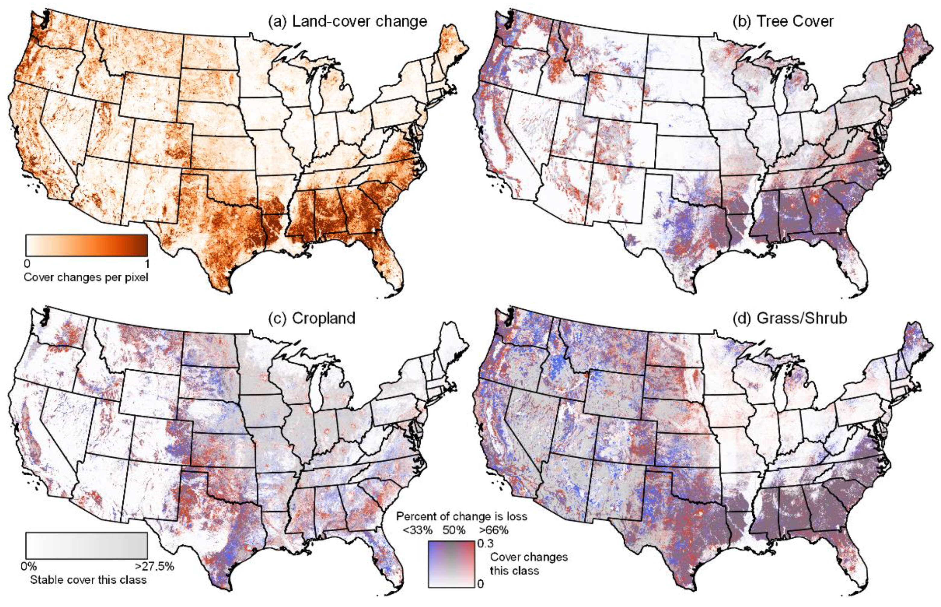
3.1. U.S. Land-Cover Change over Three Decades
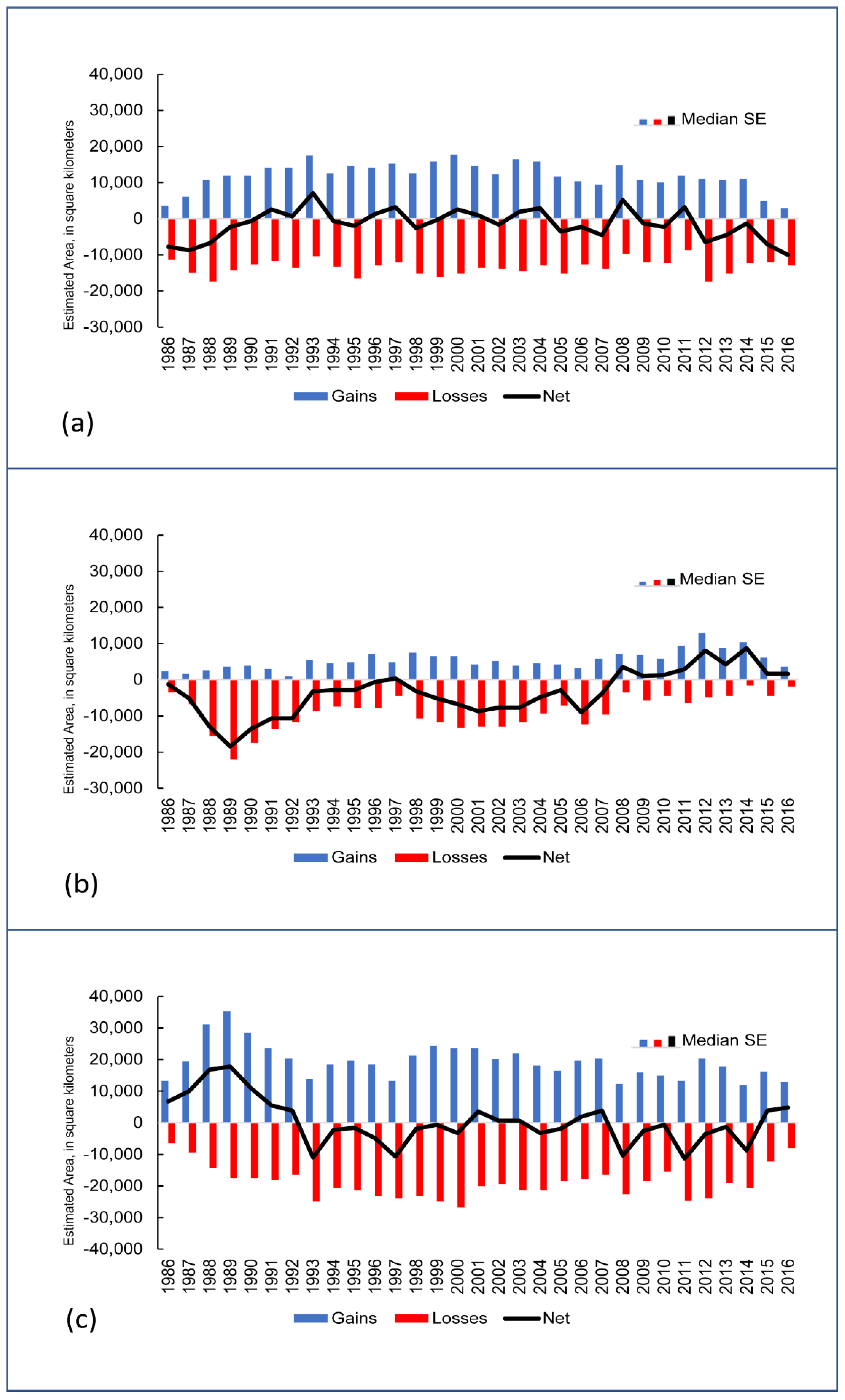
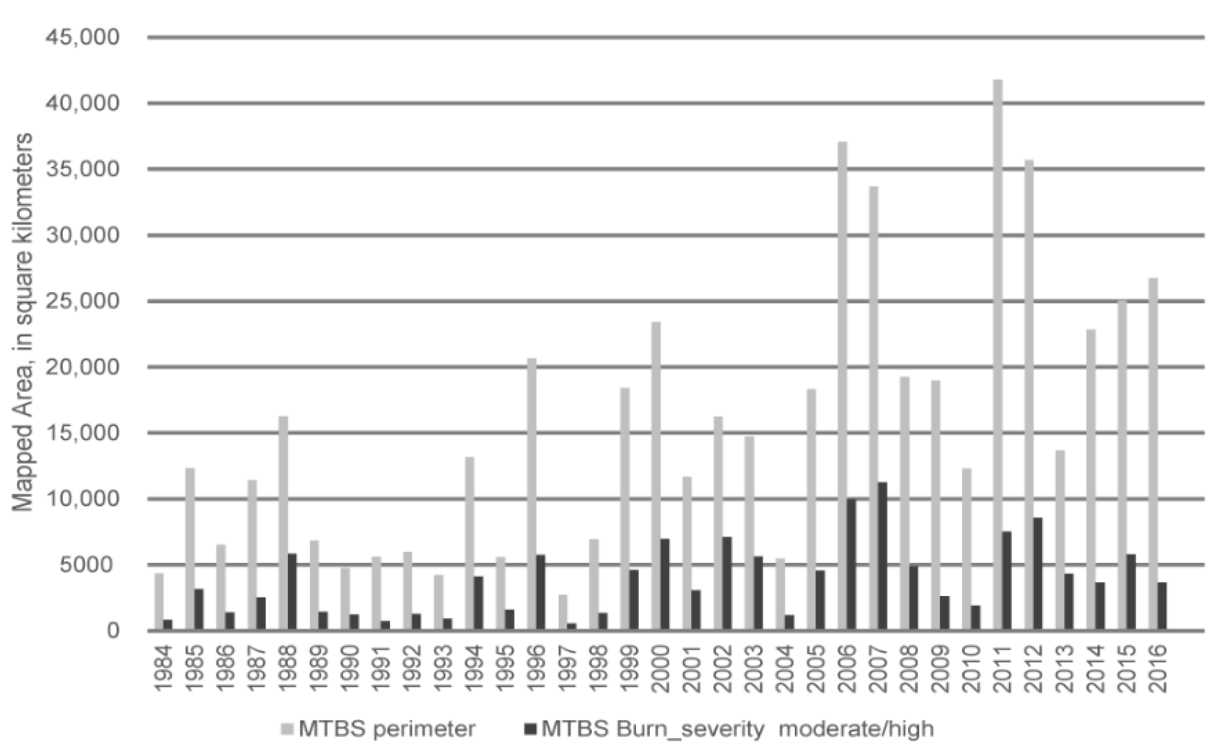
3.2. Natural Resource Cycles
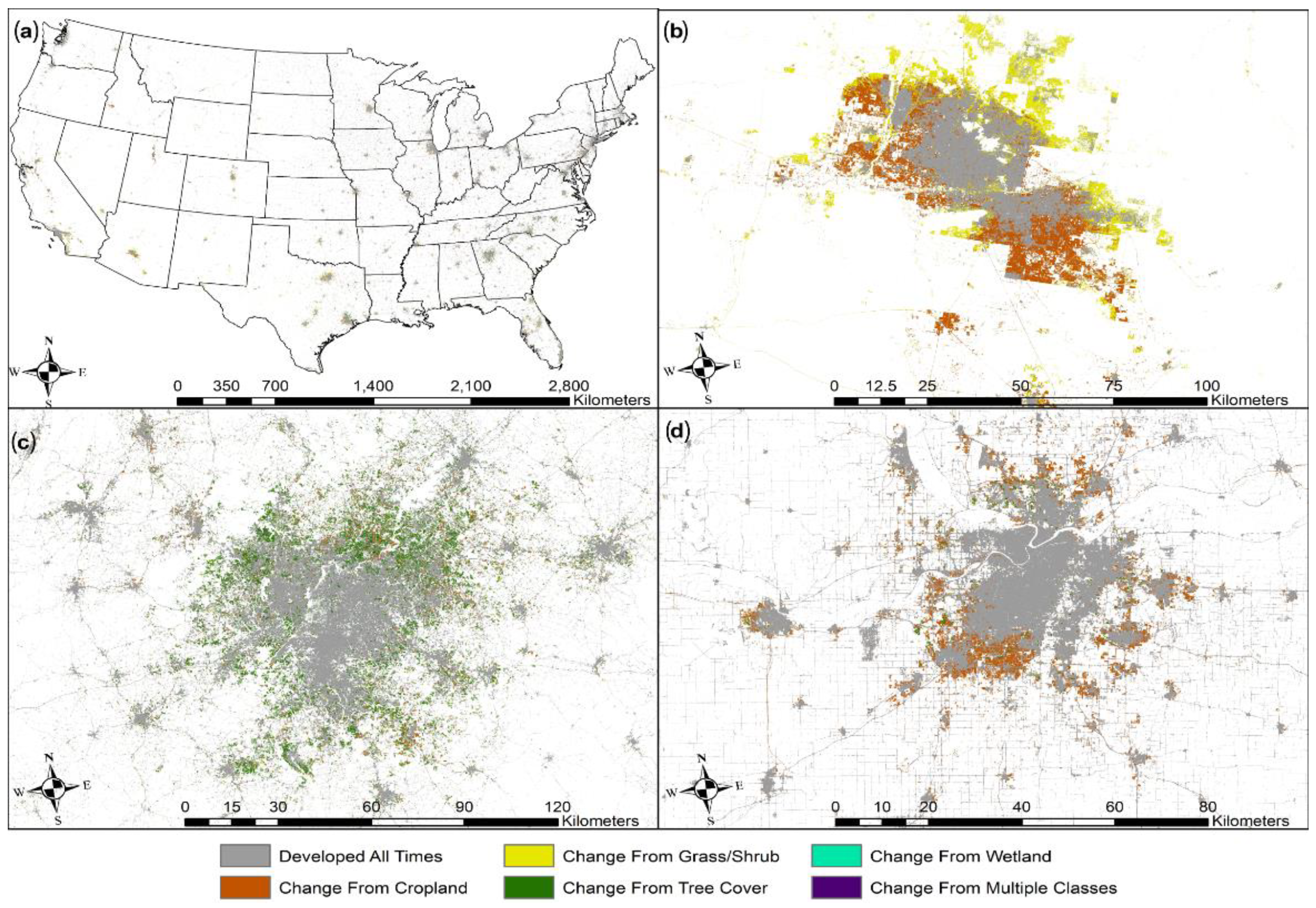
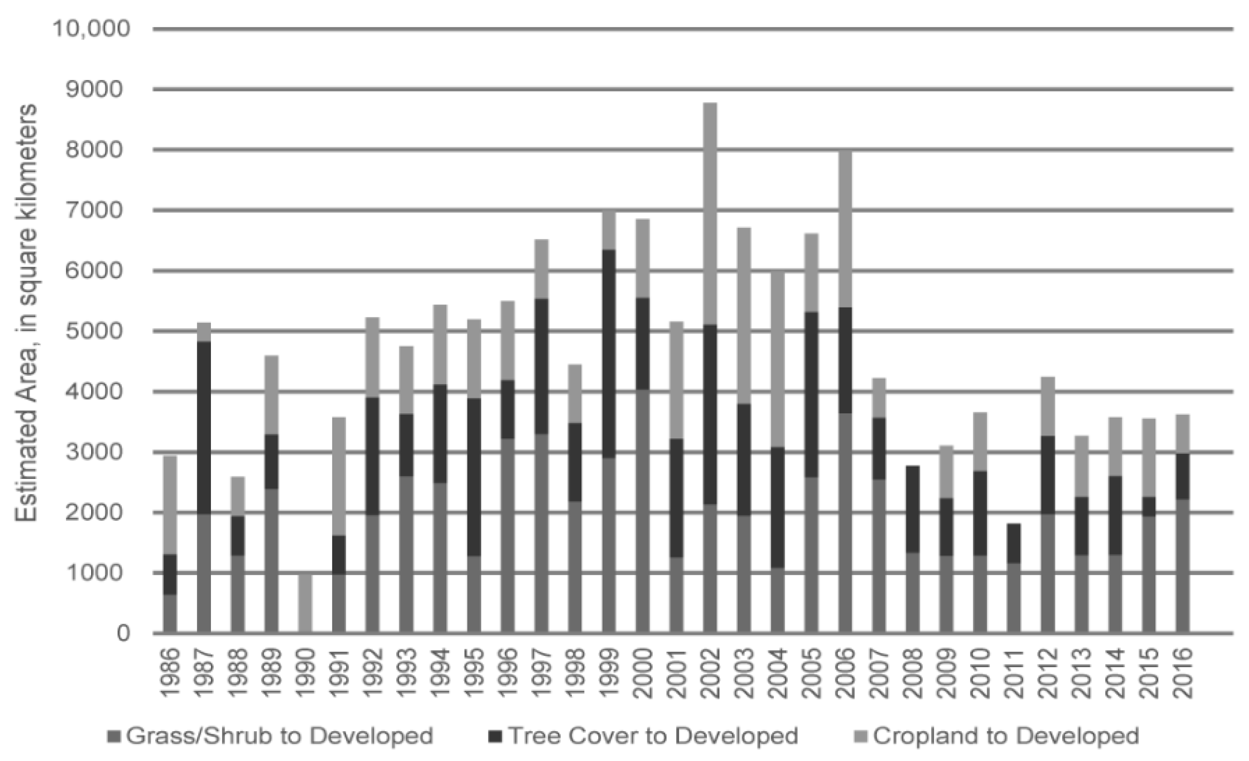
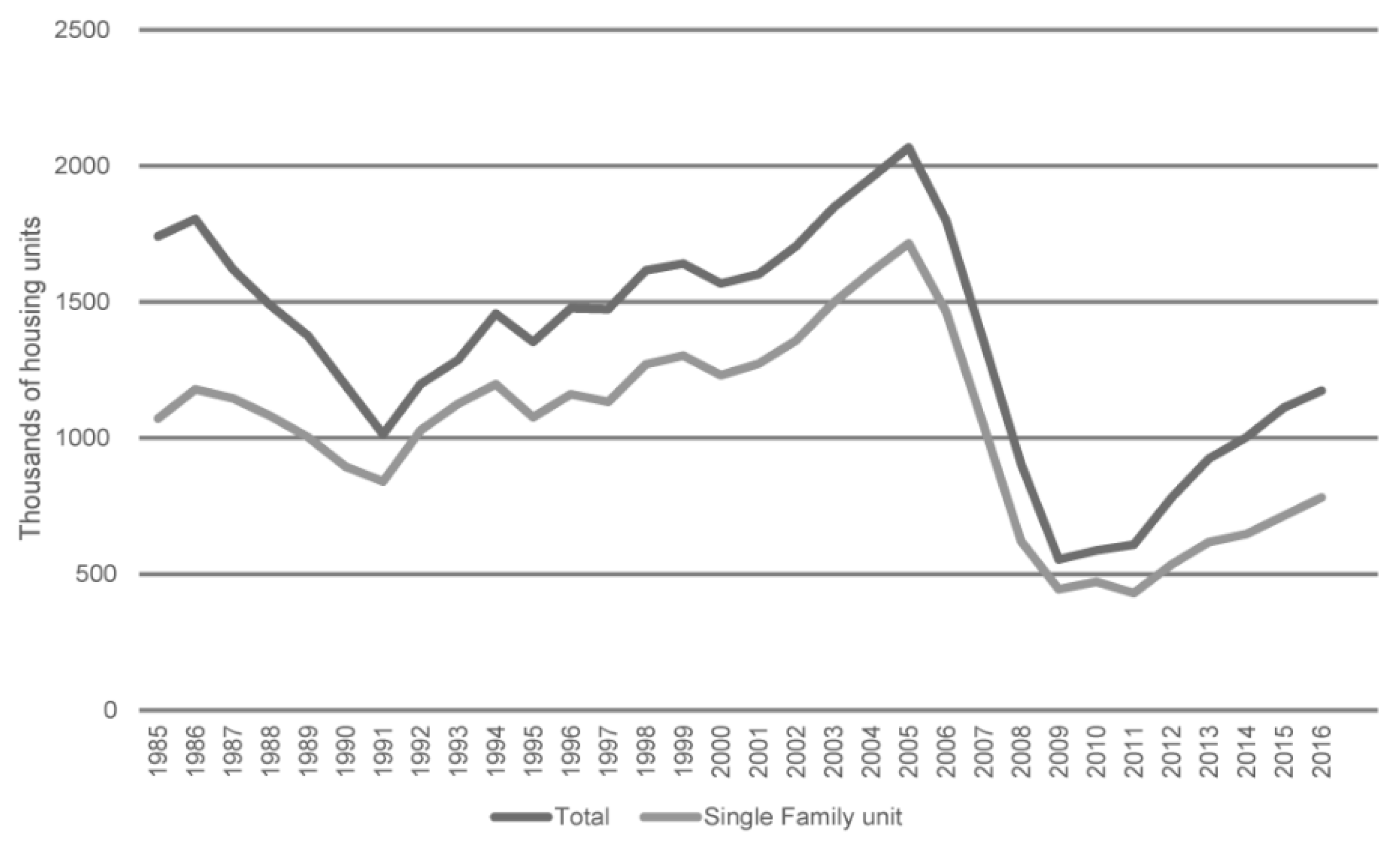
3.3. Developed Land-Cover Change
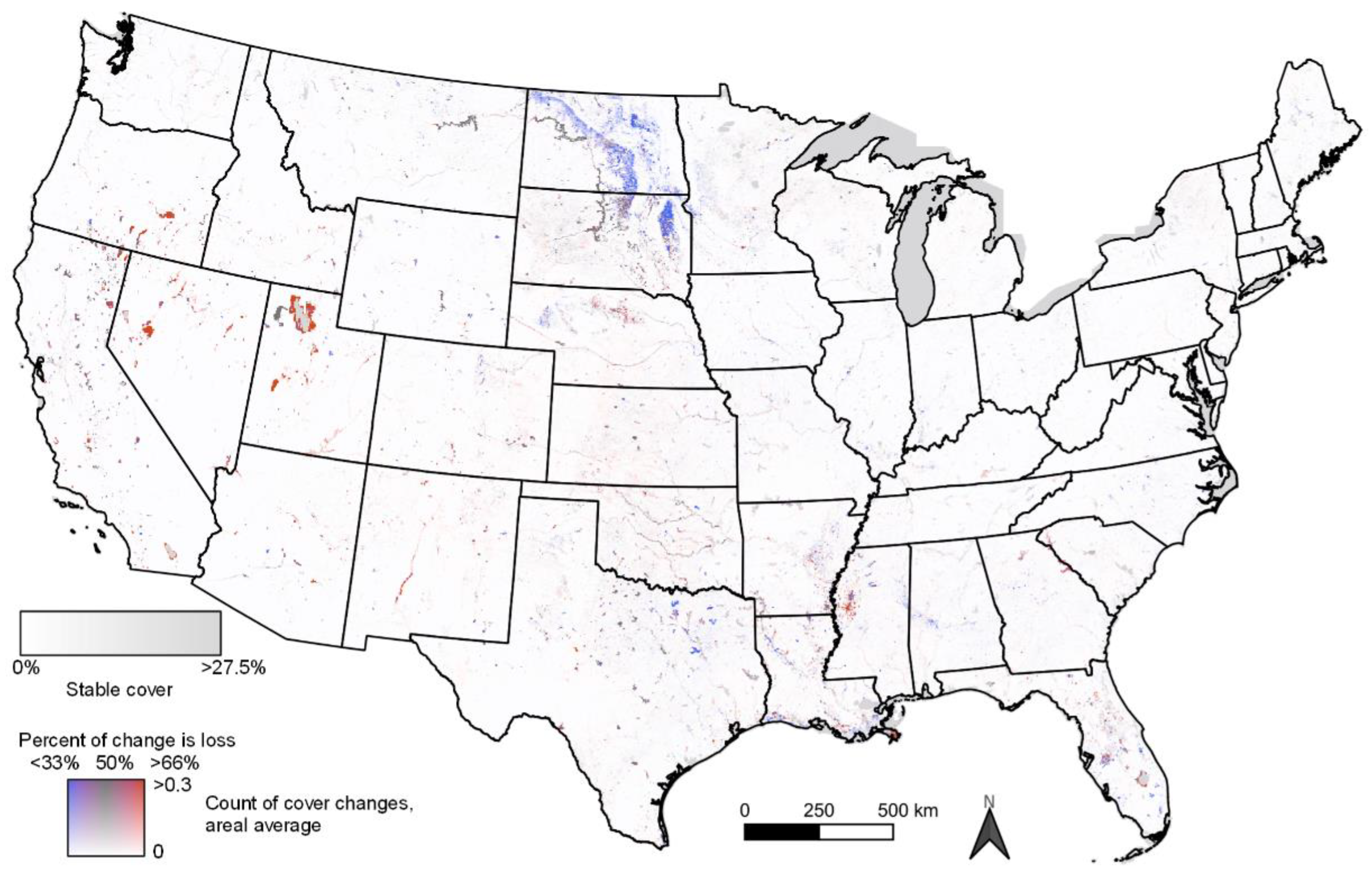
3.4. Surface-Water Dynamics
4. Discussion and Conclusions
Supplementary Materials
Author Contributions
Funding
Data Availability Statement
Acknowledgments
Conflicts of Interest
Appendix A

| Land-Cover Class Definition | |
|---|---|
| Developed | Areas of intensive use with much of the land covered with structures (e.g., high density residential, commercial, industrial, or transportation), or less intensive uses where the land-cover matrix includes vegetation, bare ground, and structures (e.g., low density residential, recreational facilities, cemeteries, transportation/utility corridors), including any land functionally related to the developed or built-up activity. |
| Cropland | Land in either a vegetated or unvegetated state used in production of food, fiber, and fuels. This includes cultivated and uncultivated croplands, hay lands, orchards, vineyards, and confined livestock operations. Forest plantations are considered as forests or woodlands (Tree Cover class) regardless of the use of the wood products. |
| Grass/Shrub | Land predominantly covered with shrubs and perennial or annual natural and domesticated grasses (e.g., pasture), forbs, or other forms of herbaceous vegetation. The grass and shrub cover must comprise at least 10% of the area and tree cover is less than 10% of the area. |
| Tree Cover | Tree-covered land where the tree-cover density is greater than 10%. Cleared or harvested trees (i.e., clearcuts) will be mapped according to current cover (e.g., Barren, Grass/Shrub). |
| Water | Areas covered with water, such as streams, canals, lakes, reservoirs, bays, or oceans. |
| Wetland | Where water saturation is the determining factor in soil characteristics, vegetation types, and animal communities. Wetlands are composed of mosaics of water, bare soil, and herbaceous or wooded vegetated cover. |
| Ice/Snow | Land where accumulated snow and ice does not completely melt during the summer period (i.e., perennial ice/snow). |
| Barren | Land composed of natural occurrences of soils, sand, or rocks where less than 10% of the area is vegetated. |
References
- Homer, C.; Dewitz, J.; Jin, S.; Xian, G.; Costello, C.; Danielson, P.; Gass, L.; Funk, M.; Wickham, J.; Stehman, S.; et al. Conterminous United States land cover change patterns 2001–2016 from the 2016 National Land Cover Database. ISPRS J. Photogramm. Remote Sens. 2020, 162, 184–199. [Google Scholar] [CrossRef]
- Marques, A.; Martins, I.S.; Kastner, T.; Plutzer, C.; Theurl, M.C.; Eisenmenger, N.; Huijbregts, M.A.J.; Wood, R.; Stadler, K.; Bruckner, M.; et al. Increasing impacts of land use on biodiversity and carbon sequestration driven by population and economic growth. Nat. Ecol. Evol. 2019, 3, 628–637. [Google Scholar] [CrossRef]
- Loveland, T.R.; Acevedo, W.; Sayler, K.L. Land-Cover Trends in the Eastern United States—1973 to 2000. In Status and Trends of Land Change in the Eastern United States—1973 to 2000; Sayler, K.L., Acevedo, W., Taylor, J.L., Auch, R.F., Eds.; US Department of the Interior, US Geological Survey: Washington, DC, USA, 2016; pp. 3–16. [Google Scholar] [CrossRef] [Green Version]
- McDonald, R.I.; Weber, K.F.; Padowski, J.; Boucher, T.; Shemie, D. Estimating watershed degradation over the last century and its impact on water-treatment costs for the world’s large cities. Proc. Natl. Acad. Sci. USA 2016, 113, 9117–9122. [Google Scholar] [CrossRef] [PubMed] [Green Version]
- Modernel, P.; Rossing, W.A.H.; Corbeels, M.; Dogliotti, S.; Picasso, V.; Tittonell, P. Land use change and ecosystem service provision in Pampas and Campos grasslands of southern South America. Environ. Res. Lett. 2016, 11, 113002. [Google Scholar] [CrossRef]
- Law, B.E.; Hudiburg, T.W.; Berner, L.T.; Kent, J.J.; Buotte, P.C.; Harmon, M.E. Land use strategies to mitigate climate change in carbon dense temperate forests. Proc. Natl. Acad. Sci. USA 2018, 115, 3663–3668. [Google Scholar] [CrossRef] [Green Version]
- Ouyang, Y.; Leininger, T.D.; Moran, M. Impacts of reforestation upon sediment load and water outflow in the Lower Yazoo River watershed, Mississippi. Ecol. Eng. 2013, 61, 394–406. [Google Scholar] [CrossRef]
- Hille, S.; Andersen, D.K.; Kronvang, B.; Baattrup-Pedersen, A. Structural and functional characteristics of buffer strip vegetation in an agricultural landscape—High potential for nutrient removal but low potential for plant biodiversity. Sci. Total Environ. 2018, 628–629, 805–814. [Google Scholar] [CrossRef]
- Lind, L.; Hasselquist, E.M.; Laudon, H. Towards ecologically functional riparian zones: A meta-analysis to develop guidelines for protecting ecosystem functions and biodiversity in agricultural landscapes. J. Environ. Manag. 2019, 249, 109391. [Google Scholar] [CrossRef]
- Bigelow, D.P.; Borchers, A. Major Uses of Land in the United States, 2012; United States Department of Agriculture Economic Research Service: Washington, DC, USA, 2012.
- Brown, J.F.; Tollerud, H.J.; Barber, C.P.; Zhou, Q.; Dwyer, J.L.; Vogelmann, J.E.; Loveland, T.R.; Woodcock, C.E.; Stehman, S.V.; Zhu, Z.; et al. Lessons learned implementing an operational continuous United States national land change monitoring capability—The Land Change Monitoring, Assessment, and Projection (LCMAP) approach. Remote Sens. Environ. 2020, 238, 111356. [Google Scholar] [CrossRef]
- Loveland, T.R.; Sohl, T.L.; Stehman, S.V.; Gallant, A.L.; Sayler, K.L.; Napton, D.E. A strategy for estimating the rates of recent United States land-cover changes. Photogramm. Eng. Remote Sens. 2002, 68, 1091–1099. [Google Scholar]
- Estes, J.E.; Loveland, T.R. Toward the use of remote sensing and other data to delineate functional types in terrestrial and aquatic systems. Dev. Atmos. 1999, 24, 125–150. [Google Scholar] [CrossRef]
- Wulder, M.A.; White, A.C.; Goward, S.N.; Masek, J.G.; Irons, J.R.; Herold, M.; Cohen, W.B.; Loveland, T.R.; Woodcock, C.E. Landsat continuity: Issues and opportunities for land cover monitoring. Remote Sens. Environ. 2008, 112, 955–969. [Google Scholar] [CrossRef]
- Woodcock, C.E.; Allen, R.; Anderson, M.; Belward, A.; Bindschadler, R.; Cohen, W.; Gao, F.; Goward, S.N.; Helder, D.; Helmer, E.; et al. Free access to Landsat imagery. Science 2008, 320, 1011. [Google Scholar] [CrossRef] [PubMed]
- Wulder, M.A.; Masek, J.G.; Cohen, W.B.; Loveland, T.R.; Woodcock, C.E. Opening the archive—How free data has enabled the science and monitoring promise of Landsat. Remote Sens. Environ. 2013, 122, 2–10. [Google Scholar] [CrossRef]
- Zhu, Z.; Woodcock, C.E. Continuous change detection and classification of land cover using all available Landsat data. Remote Sens. Environ. 2014, 144, 152–171. [Google Scholar] [CrossRef] [Green Version]
- Zhu, Z.; Gallant, A.L.; Woodcock, C.E.; Pengra, B.; Olofsson, P.; Loveland, T.R.; Jin, S.; Dahal, D.; Yang, L.; Auch, R.F. Optimizing selection of training and auxiliary data for operational land cover classification for the LCMAP initiative. ISPR J. Photogramm. Remote Sens. 2016, 122, 206–221. [Google Scholar] [CrossRef] [Green Version]
- Chen, L.; Dirmeyer, P.A. Impacts of land-use/land-cover change on afternoon precipitation over North America. J. Clim. 2017, 30, 2121–2140. [Google Scholar] [CrossRef]
- Liu, J.; Sleeter, B.M.; Zhu, Z.; Loveland, T.R.; Sohl, T.; Howard, S.M.; Key, C.H.; Hawbaker, T.; Liu, S.; Reed, B.; et al. Critical land change information enhances the understanding of carbon balance in the United States. Glob. Chang. Biol. 2020, 26, 3920–3929. [Google Scholar] [CrossRef]
- Li, C.; Sun, G.; Caldwell, P.V.; Cohen, E.; Fang, Y.; Zhang, Y.; Oudin, L.; Sanchez, G.M.; Meentemeyer, R.K. Impacts of urbanization on watershed water balances across the conterminous United States. Water Resour. Res. 2020, 56, e2019WR026574. [Google Scholar] [CrossRef]
- Moisen, G.G.; McConville, K.S.; Schroeder, T.A.; Healey, S.P.; Finco, M.V.; Frescino, T.S. Estimating land use and land cover change in north central Georgia: Can remote sensing observations augment traditional forest inventory data? Forests 2020, 11, 856. [Google Scholar] [CrossRef]
- Rodgers, W.; Mahmood, R.; Leeper, R.; Yan, J. Land cover change, surface mining, and their impacts on a heavy rain event in the Appalachia. Ann. Am. Assoc. Geogr. 2018, 108, 1187–1209. [Google Scholar] [CrossRef]
- Rittenhouse, C.D.; Pidegeon, A.M.; Albright, T.P.; Culbert, P.D.; Clayton, M.K.; Flater, C.H.; Masek, J.G.; Radeloff, V.C. Land-Cover change and avian diversity in the conterminous United States. Conserv. Biol. 2012, 26, 821–829. [Google Scholar] [CrossRef] [PubMed]
- Hansen, M.C.; Egorov, A.; Potapov, P.V.; Stehman, S.V.; Tyukavina, A.; Turubanova, S.A.; Roy, D.P.; Goetz, S.J.; Loveland, T.R.; Ju, J.; et al. Monitoring conterminous United States (CONUS) land cover change with Web-Enabled Landsat Data (WELD). Remote Sens. Environ. 2014, 140, 466–484. [Google Scholar] [CrossRef] [Green Version]
- Wright, C.K.; Wimberly, M.C. Recent land use change in the Western Corn Belt threatens grasslands and wetlands. Proc. Natl. Acad. Sci. USA 2013, 110, 4134–4139. [Google Scholar] [CrossRef] [PubMed] [Green Version]
- Gong, P.; Li, X.; Wang, J.; Bai, Y.; Chen, B.; Hu, T.; Liu, X.; Xu, B.; Yang, J.; Zhang, W.; et al. Annual maps of global artificial imperious area (GAIA) between 1985 and 2018. Remote Sens. Environ. 2020, 236, 111510. [Google Scholar] [CrossRef]
- Li, Y.; Zhou, Y.; Zhu, Z.; Cao, W. A national dataset of 30 m annual urban extent dynamics (1985–2015) in the conterminous United States. Earth Sys. Sci. Data 2020, 12, 357–371. [Google Scholar] [CrossRef] [Green Version]
- US Department of Agriculture. Summary Report: 2017 National Resources Inventory, Natural Resources Conservation Service, Washington, DC, and Center for Survey Statistics and Methodology; Iowa State University: Ames, IA, USA, 2020. Available online: https://www.nrcs.usda.gov/wps/portal/nrcs/main/national/technical/nra/nri/results/ (accessed on 10 September 2021).
- Lark, T.J.; Salmon, J.M.; Gibbs, H.K. Cropland expansion outpaces agricultural and biofuel policies in the United States. Environ. Res. Lett. 2015, 10, 044003. [Google Scholar] [CrossRef] [Green Version]
- Radwan, T.M.; Blackburn, G.A.; Whyatt, J.D.; Atkinson, P.M. Global land cover trajectories and transitions. Sci. Rep. 2021, 11, 12814. [Google Scholar] [CrossRef]
- Sleeter, B.M.; Sohl, T.L.; Loveland, T.R.; Auch, R.F.; Acevedo, W.; Drummond, M.A.; Sayler, K.L.; Stehman, S.V. Land-Cover change in the conterminous United States from 1973 to 2000. Glob. Environ. Chang. 2013, 23, 733–748. [Google Scholar] [CrossRef] [Green Version]
- Pontius, R.G., Jr.; Krithivasan, R.; Sauls, L.; Yan, Y.; Zhang, Y. Methods to summarize change among land categories across time intervals. J. Land Use Sci. 2017, 12, 218–230. [Google Scholar] [CrossRef]
- Pengra, B.W.; Stehman, S.V.; Horton, J.A.; Dockter, D.J.; Schroeder, T.A.; Yang, Z.; Cohen, W.B.; Healey, S.P.; Loveland, T.R. Quality control and assessment of interpreter consistency of annual land cover reference data in an operational national monitoring program. Remote Sens. Environ. 2020, 238, 111261. [Google Scholar] [CrossRef]
- Cohen, W.B.; Yang, Z.; Kennedy, R. Detecting trends in forest disturbance and recovery using yearly Landsat time series: 2. TimeSync—Tools for calibration and validation. Remote Sens. Environ. 2010, 114, 2911–2924. [Google Scholar] [CrossRef]
- Pengra, B.W.; Stehman, S.V.; Horton, J.A.; Wellington, D.F. LCMAP Collection 1 Annual Land Cover and Land Cover Change Validation Tables. U.S. Geol. Surv. Data Release 2020. [Google Scholar] [CrossRef]
- Stehman, S.V.; Pengra, B.W.; Horton, J.A.; Wellington, D.F. Validation of the U.S. Geological Survey’s Land Change Monitoring, Assessment and Projection (LCMAP) collection 1.0 annual land cover products 1985–2017. Remote Sens. Environ. 2021, 265, 112646. [Google Scholar] [CrossRef]
- Olofsson, P.; Foody, G.M.; Herold, M.; Stehman, S.V.; Woodcock, C.E.; Wulder, M.A. Good practices for estimating area and assessing accuracy of land change. Remote Sens. Environ. 2014, 148, 42–57. [Google Scholar] [CrossRef]
- Cochran, W.G. Sampling Techniques, 3rd ed.; Wiley: New York, NY, USA, 1977; p. 413. [Google Scholar]
- Stehman, S.V. Estimating area from an accuracy assessment error matrix. Remote Sens. Environ. 2013, 132, 202–211. [Google Scholar] [CrossRef]
- Oswalt, S.N.; Smith, W.B.; Miles, P.D.; Pugh, S.A. Forest Resources of the United States, 2017: A technical document supporting the Forest Service 2020 RPA Assessment. USDA USFS Gen. Tech. Rep. 2019, 97, 223. [Google Scholar] [CrossRef] [Green Version]
- Wright Parmenter, A.; Hansen, A.; Kennedy, R.E.; Cohen, W.; Langner, U.; Lawrence, R.; Maxwell, B.; Gallant, A.; Aspinall, R. Land use and land cover change in the greater Yellowstone ecosystem: 1975–1995. Ecol. Appl. 2003, 13, 687–703. [Google Scholar] [CrossRef]
- Cox, T.R. The Lumberman’s Frontier: Three Centuries of Land Use, Society, and Change in America’s Forests; Oregon State University Press: Corvallis, OR, USA, 2010; p. 510. [Google Scholar]
- Wear, D.N.; Greis, J.G. (Eds.) The Southern Forest Futures Project: Technical Report; Gen. Tech. Rep. SRS-GTR-178; United States Department of Agriculture, Forest Service, Southern Research Station: Asheville, NC, USA, 2013; 542p. [Google Scholar] [CrossRef]
- Berg, E.; Morgan, T.; Simmons, E. Timber Products Output (TPO)—Forest Inventory, Timber Harvest, Mill and Logging Residue—Essential Feedstock Information Needed to Characterize the NARA Supply Chain, Final Report; Northwest Advanced Renewables Alliance; Washington State University: Pullman, WA, USA, 2016; Available online: http://www.bber.umt.edu/pubs/forest/biomass/NARATimberProdOutputfinal.pdf (accessed on 17 November 2020).
- USGS; USFS. Burned Area Boundaries Dataset 1984–2017. Monitoring Trends in Burn Severity. Available online: https://mtbs.gov/direct-download (accessed on 13 April 2020).
- Dwomoh, F.K.; Brown, J.F.; Tollerud, H.J.; Auch, R.F. Hotter drought escalates tree cover declines in blue oak woodlands of California. Front. Clim. 2021, 3, 689945. [Google Scholar] [CrossRef]
- Laingen, C.R. A geo-temporal analysis of the conservation reserve program: Net vs. gross change, 1986–2013. Pap. Appl. Geogr. 2013, 36, 37–46. [Google Scholar]
- USDA; FSA. CRP Enrollment and Rental Payment by State, 1986–2018 (xls). Available online: https://www.fsa.usda.gov/programs-and-services/conservation-programs/reports-and-statistics/conservation-reserve-program-statistics/index (accessed on 13 April 2020).
- Soulard, C.E.; Wilson, T.S. Recent land-use/land-cover change in the central California Valley. J. Land Use Sci. 2015, 10, 59–80. [Google Scholar] [CrossRef] [Green Version]
- Brown, J.F.; Pervez, M.S. Merging remote sensing data and national agricultural statistics to model change in irrigated agriculture. Agric. Syst. 2014, 127, 28–40. [Google Scholar] [CrossRef] [Green Version]
- Auch, R.F.; Xian, G.; Laingen, C.R.; Sayler, K.L.; Reker, R.R. Human drivers, biophysical changes, and climatic variation affecting contemporary cropping proportions in the northern prairie of the U.S. J. Land Use Sci. 2018, 13, 32–58. [Google Scholar] [CrossRef]
- USDA; ERS. Major Land Uses, Summary Table 3: Cropland Used for Crops: Cropland Harvested (including Double-Cropped), Crop Failure, and Cultivated Summer Fallow for the United States, Annual, 1910–2019. Available online: https://www.ers.usda.gov/webdocs/DataFiles/52096/Summary_Table_1_major_uses_of_land_by_region_and_state_2012.xls?v=0 (accessed on 28 September 2021).
- USGAO. 1983 Payment-in-Kind Program Overview: Its Design, Impact, and Cost; RCED-85-89. 1985. Available online: https://www.gao.gov/products/rced-85-89 (accessed on 28 September 2021).
- USDA; FSA. Farmable Wetlands Program. Available online: https://www.fsa.usda.gov/programs-and-services/conservation-programs/farmable-wetlands/index (accessed on 14 April 2020).
- USDA; NRCS. Wetland Conservation Provisions (Swampbuster). Available online: https://www.nrcs.usda.gov/wps/portal/nrcs/detailfull/national/programs/alphabetical/camr/?cid=stelprdb1043554. (accessed on 14 April 2020).
- Verhoeven, J.T.A.; Setter, T.L. Agricultural use of wetlands: Opportunities and limitations. Ann. Bot. 2010, 105, 155–163. [Google Scholar] [CrossRef] [Green Version]
- USCB. Map-U.S. Metropolitan and Micropolitan Counties. 2017. Available online: https://www2.census.gov/geo/maps/metroarea/us_wall/Aug2017/cbsa_us_0817.pdf?# (accessed on 14 April 2020).
- USCB. U.S. Population by Year, July 1 Estimates. Available online: https://www.multpl.com/united-states-population/table/by-year (accessed on 14 April 2020).
- USCB. New Residential Construction, Historical Data, Housing Unit Started (xls). Available online: https://www.census.gov/construction/nrc/historical_data/index.html (accessed on 14 April 2020).
- Lee, H. Are millennials coming to town? Residential location choice of young adults. Urban Aff. Rev. 2020, 56, 564–604. [Google Scholar] [CrossRef]
- Liu, G.; Schwartz, F.W. An integrated observational and model-based analysis of the hydrologic response of prairie pothole systems to variability in climate. Water Resour. Res. 2011, 47, W02504. [Google Scholar] [CrossRef]
- Todhunter, P.E. A volumetric water budget of Devils Lake (USA): Non-Stationary precipitation–runoff relationships in an amplifier terminal lake. Hydrol. Sci. J. 2018, 63, 1275–1291. [Google Scholar] [CrossRef]
- Svoboda, M.; LeComte, D.; Hayes, M.; Heim, R.; Gleason, K.; Angel, J.; Rippey, B.; Tinker, R.; Palecki, M.; Stooksbury, D.; et al. The Drought Monitor. Bull. Am. Meteorol. Soc. 2002, 83, 1181–1190. [Google Scholar] [CrossRef] [Green Version]
- Baxter, B.K.; Butler, J.K. Climate Change and Great Salt Lake. In Great Salt Lake Biology; Baxter, B.K., Butler, J.K., Eds.; Springer: Cham, Switzerland, 2020; pp. 23–52. [Google Scholar] [CrossRef]
- Roberts, S. A Rank that Rankles: New York Slips to No. 3; Now Texas is 2nd Most Populous State; The New York Times: New York, NY, USA, 19 May 1994; Section B; p. 1. [Google Scholar]
- Gooch, T.; Albright, J.; Ickert, R.A. Water availability modeling for regional water planning. In Texas in World Environmental and Water Resources Congress 2011—Bearing Knowledge for Sustainability Proceedings; Beighley, E.R., Killgore, M.W., Eds.; American Society of Civil Engineers: New York, NY, USA, 2011; pp. 2987–2996. [Google Scholar] [CrossRef]
- Kumar, G.; Engle, C.; Hegde, S.; van Senten, J. Economics of U.S. catfish farming practices: Profitability, economies of size, and liquidity. J. World Aquac. Soc. 2020, 51, 829–846. [Google Scholar] [CrossRef]
- USGS. Land Change Monitoring, Assessment, and Projection (LCMAP Data Format Control Book (DFCB): U.S. Geological Survey, LSDS 1424. 2020. Available online: https://www.usgs.gov/media/files/lcmap-dfcb (accessed on 15 December 2021).


| Land Cover | Area (km2) | SE (km2) | Area (%) | SE (%) |
|---|---|---|---|---|
| Developed | 131,209 | 6866 | 1.63 | 0.09 |
| Cropland | −109,233 | 9485 | −1.35 | 0.12 |
| Grass/Shrub | 11,311 | 12,479 | 0.14 | 0.15 |
| Tree Cover | −44,921 | 9878 | −0.56 | 0.12 |
| Water | 7756 | 3166 | 0.10 | 0.04 |
| Wetland | 970 | 2685 | 0.01 | 0.03 |
| Ice/Snow | 0 | 0 | 0.00 | 0.00 |
| Barren | 2909 | 1409 | 0.04 | 0.02 |
| Change Frequency | Area (%) | SE (%) | Area (km2) | SE (km2) |
|---|---|---|---|---|
| 0 | 88.50 | 0.18 | 7,142,174 | 14,607 |
| 1+ | 11.50 | 0.18 | 927,806 | 14,607 |
| 1 | 6.85 | 0.16 | 552,951 | 12,902 |
| 2 | 3.75 | 0.12 | 302,491 | 9700 |
| 3 | 0.52 | 0.05 | 41,690 | 3661 |
| 4 | 0.22 | 0.03 | 18,098 | 2416 |
| 5 | 0.05 | 0.01 | 3878 | 1119 |
| 6 | 0.03 | 0.01 | 2585 | 914 |
| 7 | 0.01 | 0.01 | 646 | 457 |
| 8 | 0.01 | 0.01 | 970 | 560 |
| 9 | 0.01 | 0.01 | 646 | 457 |
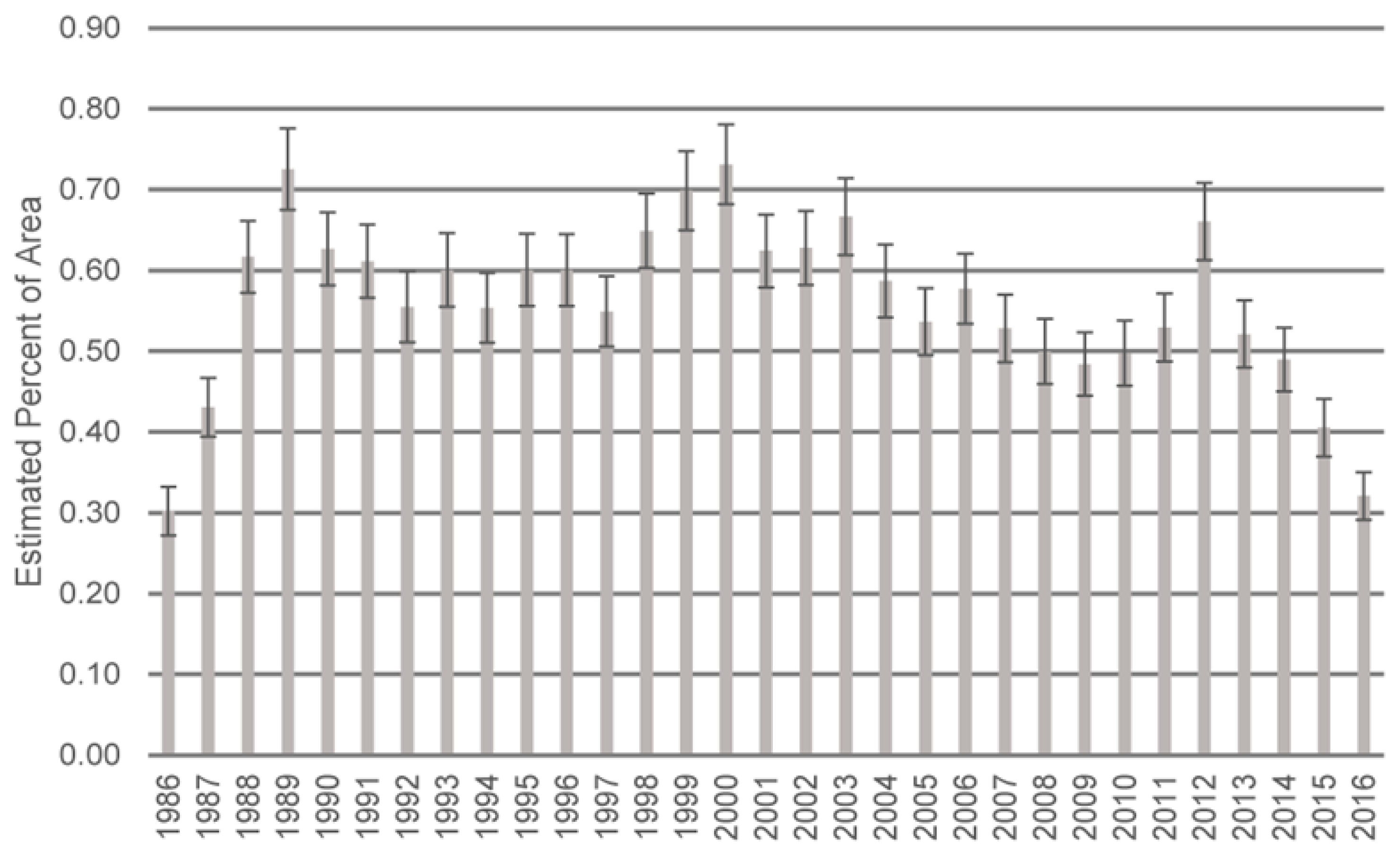
| Year | Change Area of CONUS (%) | SE Change (%) | Change Area (km2) | SE Change (km2) |
|---|---|---|---|---|
| 1986 | 0.3020 | 0.0344 | 24,374 | 2776 |
| 1987 | 0.4308 | 0.0407 | 34,764 | 3288 |
| 1988 | 0.6208 | 0.0488 | 50,097 | 3937 |
| 1989 | 0.7251 | 0.0534 | 58,518 | 4308 |
| 1990 | 0.6266 | 0.0489 | 50,566 | 3944 |
| 1991 | 0.6111 | 0.0488 | 49,319 | 3942 |
| 1992 | 0.5551 | 0.0470 | 44,796 | 3792 |
| 1993 | 0.6005 | 0.0493 | 48,459 | 3976 |
| 1994 | 0.5537 | 0.0463 | 44,681 | 3734 |
| 1995 | 0.6005 | 0.0479 | 48,463 | 3868 |
| 1996 | 0.6004 | 0.0480 | 48,454 | 3871 |
| 1997 | 0.5491 | 0.0462 | 44,314 | 3730 |
| 1998 | 0.6490 | 0.0499 | 52,376 | 4028 |
| 1999 | 0.6988 | 0.0521 | 56,390 | 4202 |
| 2000 | 0.7311 | 0.0535 | 59,004 | 4320 |
| 2001 | 0.6282 | 0.0492 | 50,693 | 3972 |
| 2002 | 0.6276 | 0.0498 | 50,650 | 4020 |
| 2003 | 0.6665 | 0.0509 | 53,790 | 4112 |
| 2004 | 0.5871 | 0.0481 | 47,380 | 3885 |
| 2005 | 0.5326 | 0.0452 | 42,980 | 3650 |
| 2006 | 0.5774 | 0.0475 | 46,598 | 3835 |
| 2007 | 0.5322 | 0.0453 | 42,952 | 3659 |
| 2008 | 0.5037 | 0.0441 | 40,650 | 3559 |
| 2009 | 0.4882 | 0.0433 | 39,397 | 3490 |
| 2010 | 0.4935 | 0.0446 | 39,827 | 3595 |
| 2011 | 0.5333 | 0.0459 | 43,039 | 3701 |
| 2012 | 0.6726 | 0.0517 | 54,277 | 4173 |
| 2013 | 0.5211 | 0.0449 | 42,050 | 3620 |
| 2014 | 0.4895 | 0.0438 | 39,504 | 3534 |
| 2015 | 0.4055 | 0.0399 | 32,720 | 3224 |
| 2016 | 0.3249 | 0.0358 | 26,221 | 2888 |
| 1986—2016 | 1,408,393 | 28,527 |
Publisher’s Note: MDPI stays neutral with regard to jurisdictional claims in published maps and institutional affiliations. |
© The authors are employees of U.S. Geological Survey (USGS), and the article is a U.S. Government Work, published by MDPI, Basel, Switzerland, with the permission of USGS. Licensee MDPI, Basel, Switzerland. This article is an open access article distributed under the terms and conditions of the Creative Commons Attribution (CC BY) license (https://creativecommons.org/licenses/by/4.0/).
Share and Cite
Auch, R.F.; Wellington, D.F.; Taylor, J.L.; Stehman, S.V.; Tollerud, H.J.; Brown, J.F.; Loveland, T.R.; Pengra, B.W.; Horton, J.A.; Zhu, Z.; et al. Conterminous United States Land-Cover Change (1985–2016): New Insights from Annual Time Series. Land 2022, 11, 298. https://doi.org/10.3390/land11020298
Auch RF, Wellington DF, Taylor JL, Stehman SV, Tollerud HJ, Brown JF, Loveland TR, Pengra BW, Horton JA, Zhu Z, et al. Conterminous United States Land-Cover Change (1985–2016): New Insights from Annual Time Series. Land. 2022; 11(2):298. https://doi.org/10.3390/land11020298
Chicago/Turabian StyleAuch, Roger F., Danika F. Wellington, Janis L. Taylor, Stephen V. Stehman, Heather J. Tollerud, Jesslyn F. Brown, Thomas R. Loveland, Bruce W. Pengra, Josephine A. Horton, Zhe Zhu, and et al. 2022. "Conterminous United States Land-Cover Change (1985–2016): New Insights from Annual Time Series" Land 11, no. 2: 298. https://doi.org/10.3390/land11020298