


The Relative Timing of Population Growth and Land Use Change—A Case Study of North Taiwan from 1990 to 2015
by
 , and
, and
Hsiao-Chien Shih
1,2,*,
Douglas A. Stow
1,
John R. Weeks
1,
Konstadinos G. Goulias
2 and
Leila M. V. Carvalho
2 1
Department of Geography, San Diego State University, San Diego, CA 92182, USA
2
Department of Geography, University of California, Santa Barbara, CA 93106, USA
*
Author to whom correspondence should be addressed.
Land 2022, 11(12), 2204; https://doi.org/10.3390/land11122204
Submission received: 23 October 2022
/
Revised: 29 November 2022
/
Accepted: 30 November 2022
/
Published: 5 December 2022
(This article belongs to the Special Issue Integrating Remote Sensing and Geospatial Big Data for Land Use Mapping and Monitoring)
Abstract
:Urban expansion is a form of land cover and land use change (LCLUC) that occurs globally, and population growth can be a driver of and be driven by LCLUC. Determining the cause–effect relationship is challenging because the temporal resolution of population data is limited by decadal censuses for most countries. The purpose of this study is to explore the relationship and relative timing between population change and land use change based on a case study of northern Taiwan from 1990 to 2015. A unique dataset on population was acquired from annually-updated governmental-based population registers maintained at the district level, and land-use expansion data (Residential, Employment, and Transportation Corridor categories) were derived from dense time series of Landsat imagery. Linear regression was applied to understand the general relationship between population and land use and their changes. The strongest relationships were found between population and areal extent of Residential land use, and between population change and Residential areal change. Lagged correlation analysis was implemented for identifying the time lag between population growth and land use change. Most districts exhibited Residential and Employment expansion prior to population growth, especially for districts in the periphery of metropolitan areas. Conversely, the core of metropolitan areas exhibited population growth prior to Residential and Employment expansion. Residential and Employment expansion were deemed to be drivers of population change, so population change was modeled with ordinary least square and geographically weighted regression with Residential and Employment expansion in both synchronized and time lag manners. Estimated population growth was found to be the most accurate when geographic differences and time lags from urban land use expansion were both incorporated.
1. Introduction
Earth scientists and demographers have been interested in land cover and land use change (LCLUC) and its associated socio-demographic change, and urban expansion is a form of LCLUC that occurs globally [1]. For the past three decades, global urban population has doubled [2], while global urban areal coverage has almost tripled [3]. Currently, over 50% of the world’s population lives in urban areas where most human economic activities occur [2], and the global population is expected to grow until 2100 [4]. Thus, urban environments and their associated human dynamics deserve more research attention for improving urban development in the future.
Many drivers can contribute to urban expansion, including population growth, economic growth, industrialization, and transportation development [5]. Reilly et al. implemented a stochastic pixel-based model to estimate urban expansion from the impacts of transportation and activity accessibility and pointed out that the expense of automobile transport led to different urban expansion patterns in the San Francisco Bay area, USA, and Bangalore, India [6]. Compared to Bangalore, automobile expenses were relatively lower in the Bay Area, and the resultant urban expansion forms are sparse over a greater geographical extent. Wu et al. applied geographically and temporally weighted regression (GTWR) to estimate urban expansion in China from 2000 to 2015 with multiple socio-economic variables and found that gross domestic product (GDP), population density, secondary industry employment, and capital investment positively contributed to urban expansion more than other variables [7]. Li et al. applied a spatial probability model to estimate whether urban expansion would occur in China from 1990 to 2010 based on socioeconomic, physical, proximity, accessibility, and neighborhood factors [8]. They indicated that the physical factors of a land parcel (e.g., elevation, slope) became less important when its environs were urbanized. Meta analyses were conducted to rank the drivers of expansion, and population growth was found to be the most critical driver of urban expansion globally [1,9].
The relationship between population and the environment is not unidirectional [10,11], and population growth (caused either by natural increase or net in-migration) can be a driver of and be driven by LCLUC. Population size and the size of human settlements showed a log-log relationship in Rondonia, Brazil [12]. Stow et al. found that population density and its change linearly impacted on the areal coverage of built-up areas at the district level in southeastern Ghana [13]. Li et al. and Wu et al. confirmed that population density is a significant driver of urban expansion in China [7,8]. Miyauchi et al. applied linear and quadratic regression to monitor the areal extent coverage based on population size within Japan for handling future population decline [14]. Thus, the area of built-up land cover is a plausible demographic indicator, especially for human population size (e.g., [12,13]). Urban expansion is often examined for five-year (e.g., [7,8]) or ten-year intervals (e.g., [13]) due to the fact that censuses often only occur with this frequency. However, these studies have failed to reveal the reciprocal processes and impacts between urban expansion and population growth. In addition, these studies used total urban area coverage as a single entity without considering that people perform activities differently for different land uses.
Urbanization is a process of more people, and a greater fraction of people, living in urban areas over time [9,15,16]. The process can be decomposed into two phenomena, urban population growth and built environment expansion. Rural-to-urban and/or urban-to-urban migration are critical sources of population growth for growing cities in addition to natural increase. Clark summarized the reasons why people move, and over 50% of the moves were associated with the desire of improved housing quality, safe neighborhoods, and accessibility to public facilities (e.g., universities, schools, and subway stations) [17]. A third of the moves resulted from life cycle changes (e.g., marriage, divorce, new or deceased household members), while the remainder of the moves stemmed from forced moving (e.g., housing eviction, wars, natural hazards) or employment change. Nevertheless, Clark pointed out that people often move due to multiple reasons and were more likely to move when they lived five miles from their workplace [17].
Massey articulated the main reasons for why people migrate from rural to urban areas [18]. First, wages in cities are higher than in traditional agrarian work, and neoclassical economic theory suggests that people are motivated to seek higher wages [19]. Second, some rural households intend to maximize their profit and lower the risk of conducting traditional cultivation, as described by household-based economic theory [20]. Third, cities need laborers to fill in the secondary sector positions for serving people who work in the primary sector based on segmented market labor theory, and unskilled, rural-to-urban migrants are attracted to fill the need for labor [21].
LCLUC occurs in both rural and urban areas due to urbanization. Massey pointed out that rural households having members who work in urban areas often spend the remittances sent home on acquiring more land in their home communities [18]. Newly purchased land either lies fallow or changes to cash crops to maximize profit. Antrop pointed out that new commercial and industrial activities may appear at the edge of large cities where new peripheral roads are developed for relieving traffic congestion during the process of urbanization [22]. Bell et al. found land abandonment due to out-migration in rural areas of Latvia, suburbanization of new luxurious housing due to in-migration of retirees to the coastal areas of Spain, and suburbanization of new illegal housing units in the Lisbon Metropolitan area [23]. However, their results were presented qualitatively with limited quantitative support for urbanization occurring at finer spatial scales, and they focused on human migration at a national scale without quantifying the impact on land use change. Li et al. and Wu et al. pointed out that urban population growth due to urban migration caused urban expansion, but they only briefly mentioned urban migration and did not quantify its magnitude [7,8].
Based on rural-to-urban theory, we hypothesize that the dominant relationships between population change and land use change in an urbanizing area occur as follows: (1) After new commercial and industrial establishments are built in a given place, job seekers from other places move to the vicinity of these establishments and primarily become renters of residential dwellings; (2) Increasing numbers of residents prompts the demand for housing, which leads to new residential developments in the place of work or nearby; (3) After the new residential buildings are completed, people can “officially” move into the new housing developments, which indicates that the migrants are officially recorded in a registered population system; and (4) Places in the process of urbanization will continue to densify with new small-scale businesses and transportation developments, and more migrants will move in. However, the latter types of land use change and human migration is not the focus of this study, as the goal is to determine whether or not most of the places (i.e., districts in this study) that were once undeveloped share similar temporal processes of land development and human in-migration at the beginning of development.
The purpose of this study is to explore the relationship and the relative timing between population change and land use change based on a case study of northern Taiwan from 1990 to 2015. This is the first study to explore and identify the relative timing between LCLUC and population migration at the annual-scale by leveraging data completeness for the study area. First, the general relationship between population, land use, and their change across space and time was tested with regression analysis. Second, the relative timing between population change and land use change was identified with lagged correlation tests. Finally, hypothetical processes of urbanization among population growth, residential, and employment land use change were validated. This study provides the first direct empirical evidence of the manner in which growth of an urban environment is associated with population growth across space and time.
2. Study Area and Study Period
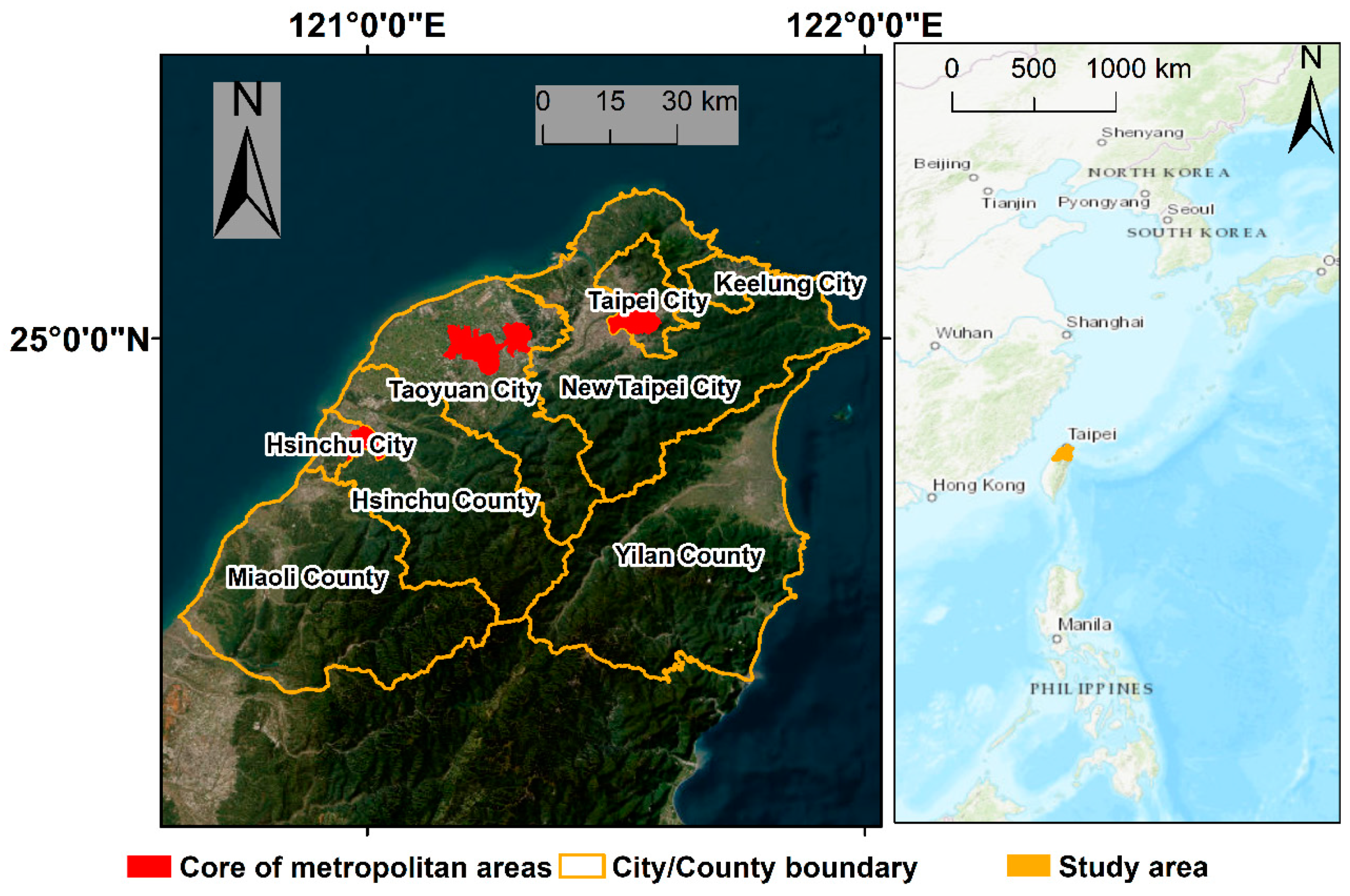
The study area is located within the northern region of Taiwan island (Figure 1), and the study period ranges from 1990 to 2015. The study area and timeframe were selected because of (1) the availability of fine spatial (district level) and temporal (annual) scale population data, and (2) the occurrence of rural-urban migration and extensive urban LCLUC during this time. The urban population keeps growing despite the continued decline in fertility rates (from a total fertility rate of 1.72 children per woman in 1990 to 1.18 in 2015). We know, then, that population growth is largely a result of rural to urban or urban to urban migration, which enables us to study the relationship of LCLUC to in-migration. Taiwan is governed by a democratic system, and land tenure and associated development receive minimal intervention by governmental agencies, except for land use zoning.
3. Materials and Methods
3.1. Materials
The data we used in this study are listed in Table 1 along with their associated spatial granularity and temporal coverage. A digital geographic information system file containing all district polygons was downloaded from a Taiwanese governmental website (https://data.gov.tw/ accessed on 1 September 2018). In total, 368 districts represent the entire Taiwan island. Within the study area, 107 districts were extracted from the downloaded shapefile, and then islets that are too small to live on and not connected to the main island of Taiwan were manually removed. The modified GIS file representing 107 districts was used as a basis for deriving areal extent of land use.
Two main sources of data were used to represent both land use and population on an annual basis. Time series data on land use from 1990 to 2015 were derived from classification of dense time series of Landsat imagery. An efficient method of estimating areal extent of three urban land-use types (Transportation Corridor, Employment, and Residential categories) in an urbanizing region over time is to generate an urban land-use change map labelled with the date that urbanization commenced, and then conduct an overlay analysis between the urban land-use change map and an accurate land-use map for the end date of the study period. Thus, a semi-automatic approach to identifying the starting time of urban land change was developed and tested based on a dense time series of Vegetation-Impervious-Soil (V-I-S) proportion maps derived from Landsat surface reflectance imagery [24]. Normalized spectra analysis was applied to estimate V-I-S proportion to reduce endmember variance and shadow in the densely built environment [25]. In total, 102 independent samples were digitized and collected in no change areas to as endmembers of the NSMA model. Later, logistic regression was applied to Landsat-derived impervious fraction time series for identifying urban expansion. An independent set of urban expansion samples based on 3 by 3 pixel units were collected from Google Earth very-high-resolution imagery to assess the accuracy of identified urban expansion. The location and estimated time for newly urbanized lands were generally accurate, with 80% of urban expansion estimated within ±2.4 years.
Next, random forest (RF) classification was applied to a Landsat image from 2015 to create maps of detailed urban land use (e.g., Residential, Employment, and Transportation categories). Residential includes pure residential and mixed use; Employment land is places where people work, including commercial, industrial, public use (e.g., governmental agencies); Transportation Corridor includes roads and railways. About 2000 training and testing polygons consisting of 500,000 Landsat pixels were manually digitized from a 2016 land use map published online by Taiwanese governmental agencies. Another independent set of samples for accuracy assessment was collected based on the same land use map, which comprises 1486 no-change, stratified random samples. Multiple input features for the RF classifier were evaluated and tested in terms of the overall map accuracy, and the input features include Landsat surface reflectance, its derivative V-I-S proportion maps, spatial arrangement of V-I-S (i.e., gray level co-occurrence matrices of V-I-S), and temporal variation of V-I-S. We found that a detailed urban land use map derived from the top 10 features with the highest RF feature importance has the highest overall accuracy. Spectral reflectance of Residential is similar to the reflectance of Employment, which causes misclassification in the resultant RF classified land use map. Additionally, accurate land use mapping with Landsat imagery within such densely built environments is quite challenging. Thus, manual editing was applied to correct misclassified pixels according to the government-published land use map, and the overall accuracy of the manually-edited land use map is 83.9% [26].
A change map was derived from the overlay analysis between the manually-edited land use map and the map of newly urbanized areas (shown in Figure 2). An additional set of 300 urban expansion samples was collected based on the government-published land use map for assessing accuracy of urban expansion along with the 1486 no change samples. The overall accuracy of 82.7% for land-use change categories, and the user’s and producer’s accuracies are shown in Table 2 [26]. The areal extents of Residential, Employment, and Transportation Corridor (Transportation hereafter) land use types were summarized for each district on an annual basis.
Two sources of population data were used, population registers and census data. The registered population data contain annual population counts at the district level. The registered population data were downloaded from Monthly Bulletin of Interior Statistics, Taiwan (R.O.C.). These data date back to 1981 on an annual basis, but district boundaries were readjusted in 1990. Thus, the registered population from 1991 to 2015 at the district level was used in the analysis. The numbers of natural increase and net migrants recorded by the population register system were published at the City/County level (i.e., the finest spatial level data that are available online) for 1992 to 2015, and the data were downloaded and used to analyze the sources of population growth. Three decadal censuses for 1990, 2000, and 2010 were also downloaded from the website of National Statistics. The census data are aggregated to the City/County level. Data from the registers and censuses were compared for consistency. Spatial-temporal trends of registered population at the district level were also analyzed.
3.2. Relationship between Population and Land Use
To understand the spatial-temporal relationships between areal extent of urban land-use types (i.e., Residential, Employment, and Transportation) and population counts (p), linear regression models were run. The models were run for population size and areal extents of land use for the same years in a synchronized manner. In addition, regression models were run between population and Urban area extent (i.e., the sum of Residential, Employment, and Transportation land uses). Annual, five-year, and ten-year changes based on the annual land-use and population data were inputs to the linear regression models. Models were run with actual data (i.e., p and land-use area in km2) as well as data normalized by district areas (i.e., population density in p/km2 and land-use areal fraction in %).
3.3. Relative Timing between Population Growth and Land-Use Expansion
The relative timing between land-use expansion and population growth was assessed using lagged correlation analysis, and each type of land use was tested exhaustively against population as a series of annual data using districts as the spatial unit of analysis. Initially, the top 30 districts with the greatest population growth or population density growth were selected for the lagged correlation analysis. Twenty-four of the top 30 population growth districts are also in the top 30 population density growth districts, so 36 districts were selected in total. Time series of population and land use are non-stationary in the temporal domain, which violates the normal distribution assumption of time series variables for any statistical test [27]. Thus, the linear growth trend of annual population and land-use data was removed before lagged correlation. Pearson’s r test was applied to each pair of L and Pd, where L is the detrended areal extent of land use, P is the detrended population count, and d represents the number of lag years, i.e., the relative timing between land-use expansion and population growth, which must satisfy the following conditions: −10 ≥ d ≥ 10 and d ∈ Z. The relative timing between land-use expansion and population growth was determined based on the d value with the highest Pearson’s r. Such a statistical test revealed whether land-use expansion tended to occur prior to population growth (i.e., d > 0), or vice versa (i.e., d < 0).
3.4. Hypothetical Processes of Urban Growth
We hypothesized two types of change sequences in terms of population change and land use change associated with urbanization in northern Taiwan. One is that Employment land (i.e., commercial and industrial areas) increases, followed by Residential land expansion, and finally population increases. This hypothetical sequence accounts for the situation that migrant workers initially commute to the newly built employment places for work from their existing homes before new construction of housing. Conversely, migrant workers could move to the existing housings in the proximities of the new employment places, and the growing population put more pressure on the local housing market over time. Construction companies observe the increase demands on housing, and new residential land use starts to appear. The other hypothetical sequence of change is Employment land increase, followed by population increases, and finally Residential land increases. For the selected 36 districts, the relative timing between population growth and Residential expansion, and relative timing between population growth and Employment expansion were identified by lagged correlation tests. Hence, the change sequences among population growth, Employment land expansion, and Residential land expansion were determined, enabling testing of the hypothesis.
4. Results
4.1. Spatial-Temporal Trends in Population and Land Use
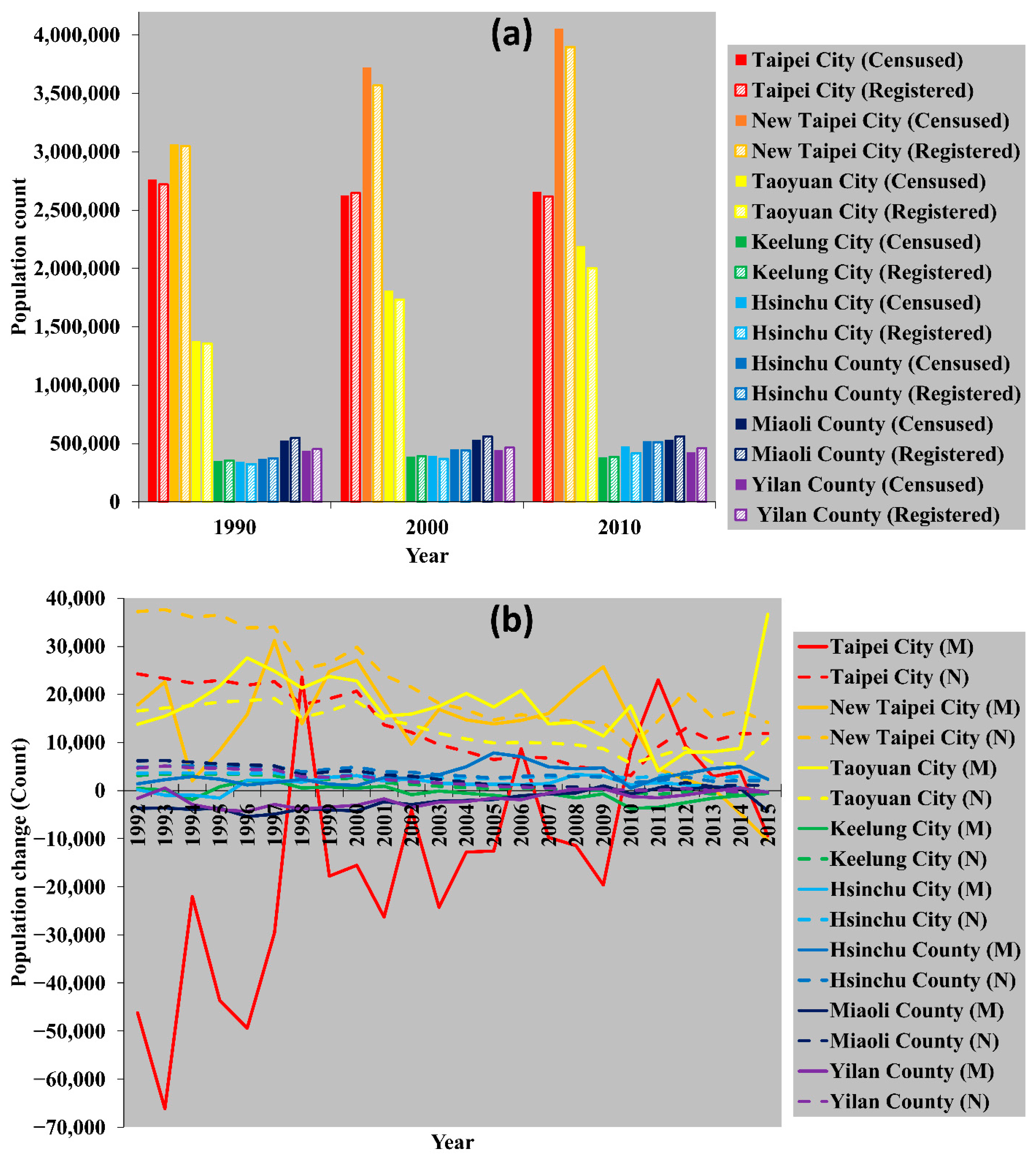
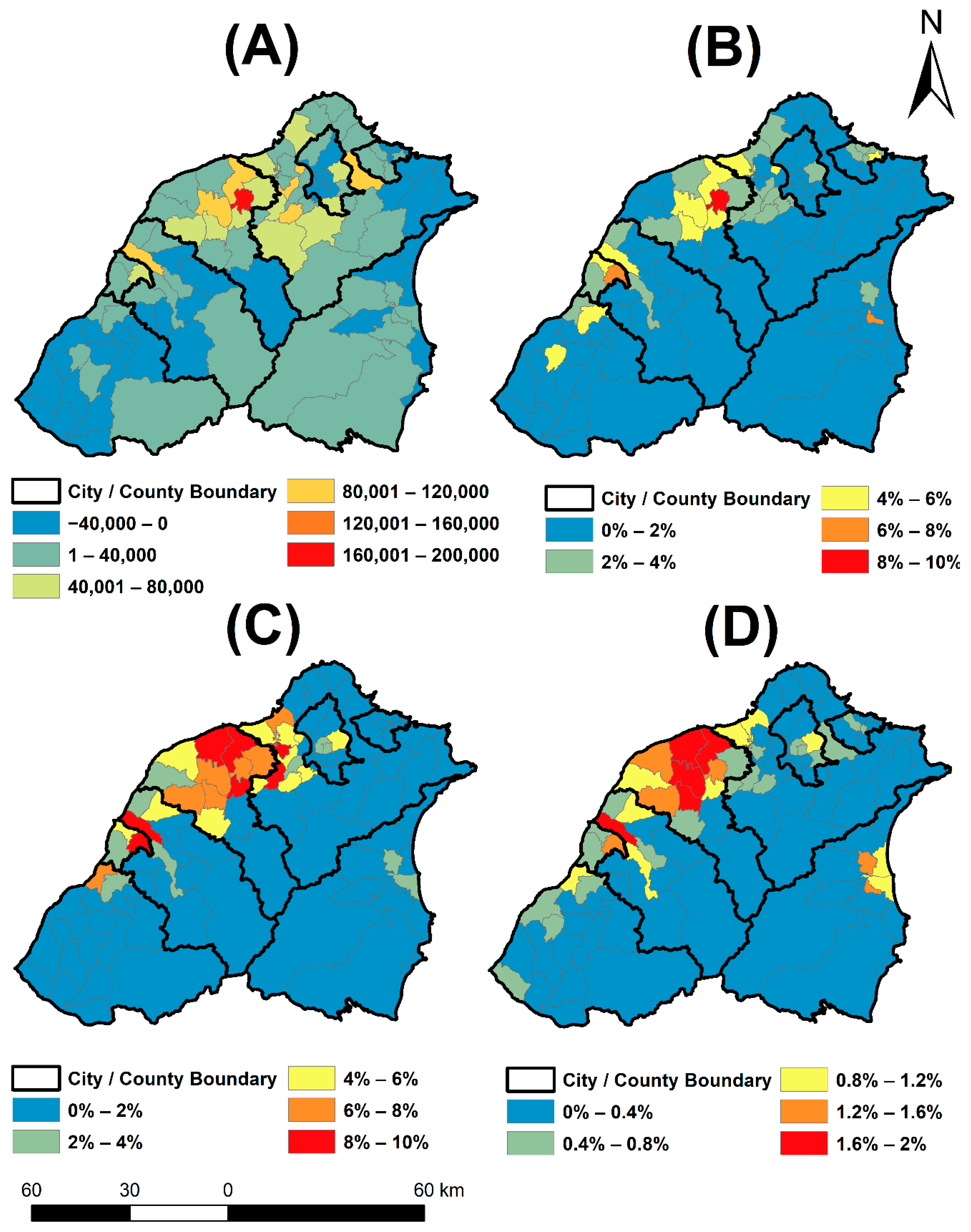
Population data from registers and censuses are compared in Figure 3. Population growth resulting from net migration is confirmed for cities and counties having higher census-enumerated populations than registered population. New Taipei, Taoyuan, Hsinchu Cities, and Hsinchu County exhibited positive net migration, while Keelung City, Miaoli, and Yilan Counties experienced out-migration. The spatial-temporal trends of registered population and land use are shown in Table 3 and Table 4, as well as in Figure 4. From 1991 to 2015, population count increased by 17,495 on average at the district level (shown in Table 3). A district in Taoyuan City experienced the greatest population growth with 181,089 more people, as shown in Table 3 and Figure 4. On average, the population density increased 330 per km2, but we found that the maximum population density dropped during the study period (shown in Table 3). Change in population density implies that urbanization is a diffusion process from urban core areas to their peripheries [22]. Of the 107 districts, 66 experienced population growth, while the remaining 41 districts exhibited population loss for the entire study period. Most districts in urban core areas and their vicinities had population growth, while districts in the urban core of Taipei City and rural areas had population loss. During the entire study period, population growth from net migration in percentage terms was 37%, 58%, 30%, and 47% for New Taipei, Taoyuan, and Hsinchu cities, and Hsinchu County, respectively (shown in Figure 3b).
The spatial-temporal trends of the three land use types that we evaluated correspond to the population dynamic trends, especially for Residential (shown in Figure 4). The three types of land use were in an expansion situation during the study period. Districts where local city halls are located tended to have higher population and urban land-use coverage than other districts. The areal extent of Employment and Transportation increased along the west coast, especially in the northern areas of Taoyuan City (Figure 4C,D). On average, districts had 1.6%, 2.2%, and 0.4% of expansion for Residential, Employment, and Transportation (shown in Table 4), respectively.
4.2. Relationship between Land Use and Population and Their Change
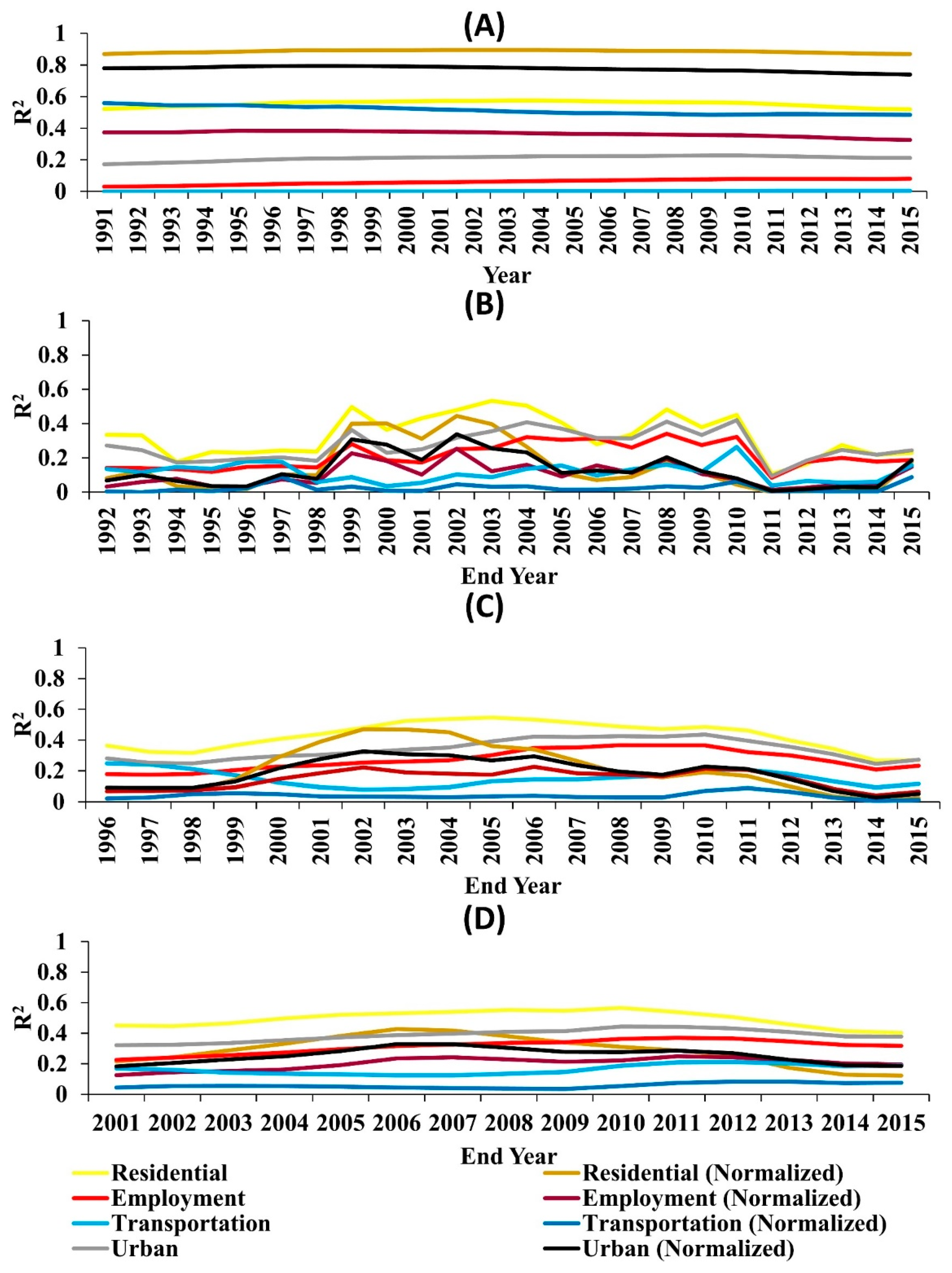
R2-values derived from the linear regression models are shown in Figure 5. Population was found to be positively related to the areal extent of land use at a statistically significant level for all land-use types. The relationship between population and Residential area is the strongest (shown in Figure 5A). R2-values are higher when population and land-use are normalized by district areas, especially for Residential. The R2-values for Transportation are moderate while the lowest for Employment. However, R2-values were trending lower over time for normalized Transportation, while relatively stable for the other two types of land use. R2-values of annual changes varied over time and are higher and more stable when the change data were derived from wider time intervals (shown in Figure 5B–D). Population change was found to be positively related to the areal change at a statistically significant level for all land use types. However, the relationship with the change data is weaker when the population and land-use changes are normalized by district areas.
4.3. Relative Timing between Population Change and Land Use Change
The relative timing between population growth and land-use expansion was identified with lagged correlation analysis applied to the 36 districts with the greatest population growth and/or population density growth (results shown in Table 5). Time lags are dispersed such that they extend from −10 to 10. According to the median of time lags, Residential land expanded 2.5 years earlier than population growth; Employment land expanded 3.5 years earlier than population growth; Transportation land expanded 1.5 years later than population growth; and General Urban land expanded 3.5 years earlier than population growth.
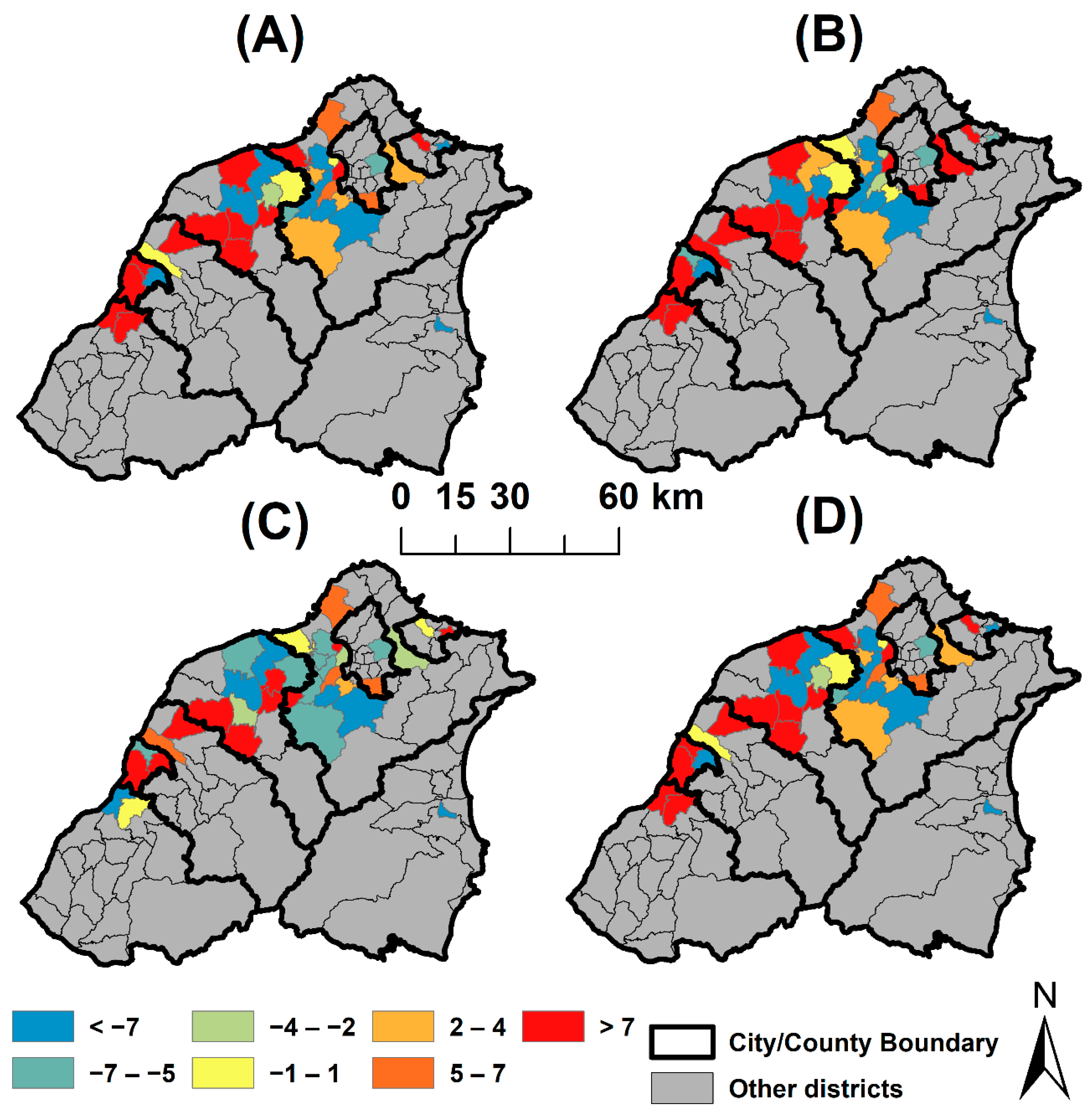
The spatial distribution of time lag for each district is shown in Figure 6. Population growth tended to occur prior to Residential and Employment expansion in the cores of Taoyuan and Hsinchu metropolitan areas (i.e., the negative time lags in Figure 6A,B) while later in the periphery of metropolitan areas (i.e., the positive time lags in Figure 6A,B). Conversely, population growth tended to occur prior to Transportation expansion in districts in the periphery of Taipei and Taoyuan metropolitan areas while later in the periphery of Hsinchu metropolitan area.
To examine differences in time lags at two administrative levels (city/county and district), the relative timing between population change and land use change was examined for Hsinchu City and its associated districts (shown in Table 6). The differences in time lags derived from East district (i.e., the urban core of Hsinchu City) were lost when the district was aggregated to Hsinchu City. Population growth occurred prior to Residential and Employment expansion in the core areas, while the urban growth sequences were reversed for suburban and peri-urban areas (i.e., North and Xianshan districts).
4.4. Model Population Change Based on Land Use Expansion
Land-use expansion (i.e., increase in area of a given land-use type) was found to occur prior to population growth for most of the 36 districts except for districts in the metropolitan cores, so land-use expansion can be inferred to be a driver of population growth, especially for Residential and Employment land expansion (shown in Figure 5D). Thus, Residential and Employment expansion were used as predictors of population change for each district of the entire study area, and four models were tested to estimate the 10-year population change related to the lowest variation in R2-values observed in Figure 5B–D. Population change during a period was modeled by an ordinary least squares (OLS) regression with inputs of the same period of Residential and Employment change (synchronized OLS). This model was used as the standard for comparison with the other three models. Time lags for population change were incorporated into the second model, and the median of time lags was used because of the dispersed distribution of time lags, as shown in Table 5. Each 10-year population change was modeled by OLS regression with Residential change three years prior and Employment change four years prior as predictors (Time lag OLS). For example, to model population change from 1995 to 2005, independent variables were Residential change from 1992 to 2002 and Employment change from 1991 to 2001.
Spatial effects related to population change were considered in a third model, and geographically weighted regression (GWR) was utilized to estimate local relationships between land use change and population change due to possible nonstationary spatial relationships among the three variables [28]. GTWR ignores the relative timing between population growth and urban expansion by simply including Residential and Employment expansion in the past and future, which is beyond the scope of this study and violates our purpose to emphasize the relative time difference. Instead, GWR was especially useful for such situations because population varied positively and negatively over space and time. Population change for a 10-year interval was modeled with GWR, and the predictors corresponded to the same period of Residential and Employment change (Synchronized GWR). We used GWR with an adaptive bandwidth based on Akaike information criterion correction (AICc) as the criterion to determine a suitable neighbor size at the district level. The time lags for Residential and Employment change were incorporated in the final model. GWR was implemented to model population change for a period with predictors of Residential change at a three-year earlier period and Employment change at a four-year earlier period (Time lag GWR).
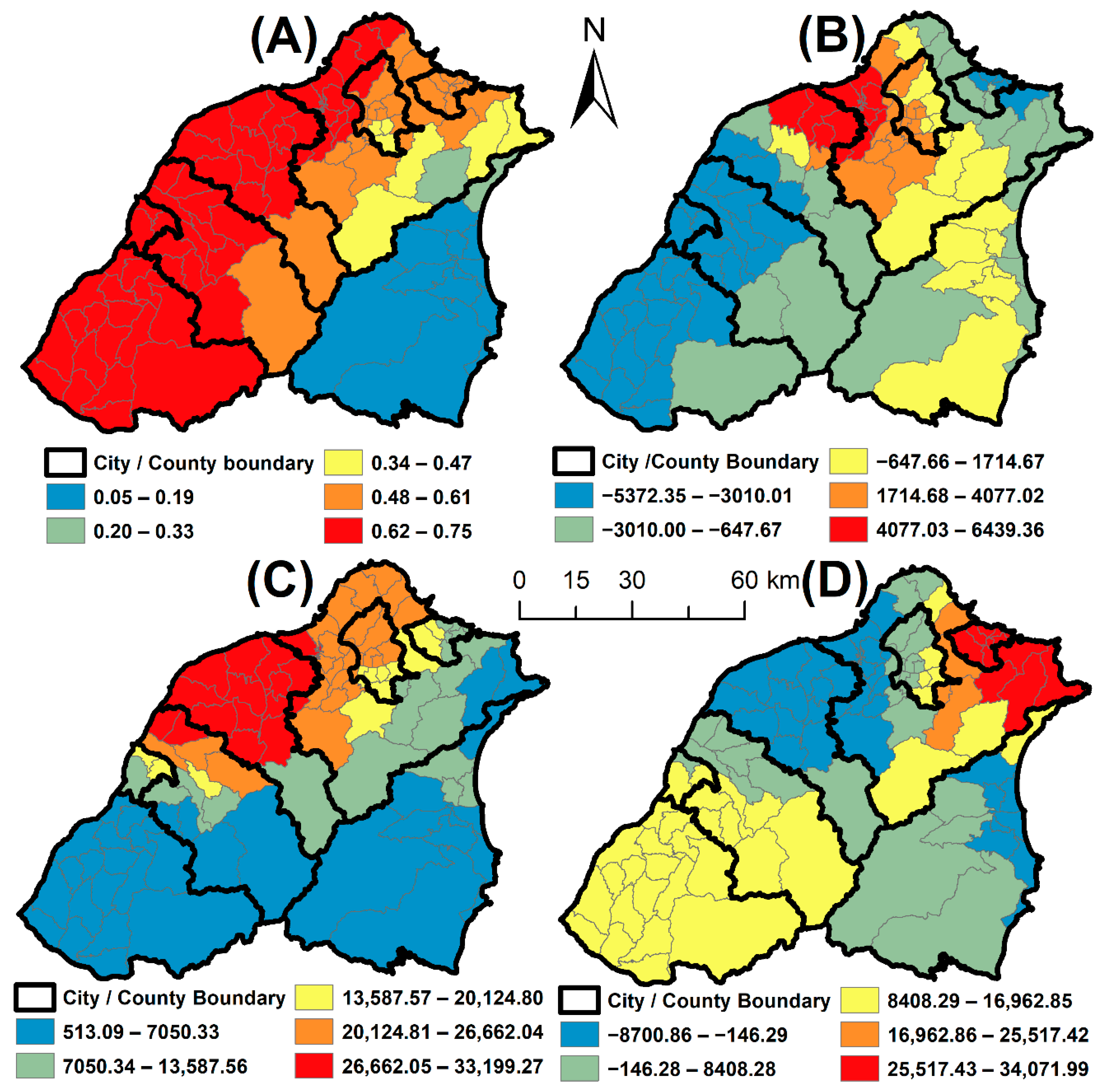
Adjusted R2-values were used to evaluate the four models, as shown in Table 7. Synchronized OLS yielded the lowest adjusted R2-values, while Time lag GWR resulted in the highest adjusted R2-values. Adjusted R2-values slightly increased when only time lag between population change and land use change was incorporated. Conversely, the adjusted R2-values substantially increased in the synchronized GWR. The synchronized and Time lag GWR models yielded statistically significant improvement compared to the Synchronized and Time lag OLS models based on ANOVA tests (p-values < 0.0001). Adjusted R2-values were substantially boosted because the districts experienced population growth or decline were modeled together with Residential and Employment changes, but the impacts from Residential and Employment changes varied over depopulating and population-growing districts. Specifically, local R2-values and coefficients of predictors of Time lag GWR only slightly vary over different time periods, and the metrics of an exemplar model of Time lag GWR (i.e., population change from 2005 to 2015) are shown in Figure 7. The local R2-values are high (local R2 > 0.62) for districts in the western part of the study area and gradually decrease to the southeast direction (Figure 7A), which implies that the local models among population change, Residential, and Employment expansion are accurate in the western part of the study area. Thus, both spatial effects and time lags between population change and land use change should be considered for future modelling of population change with land-use change as predictors.
4.5. Hypothesis Testing
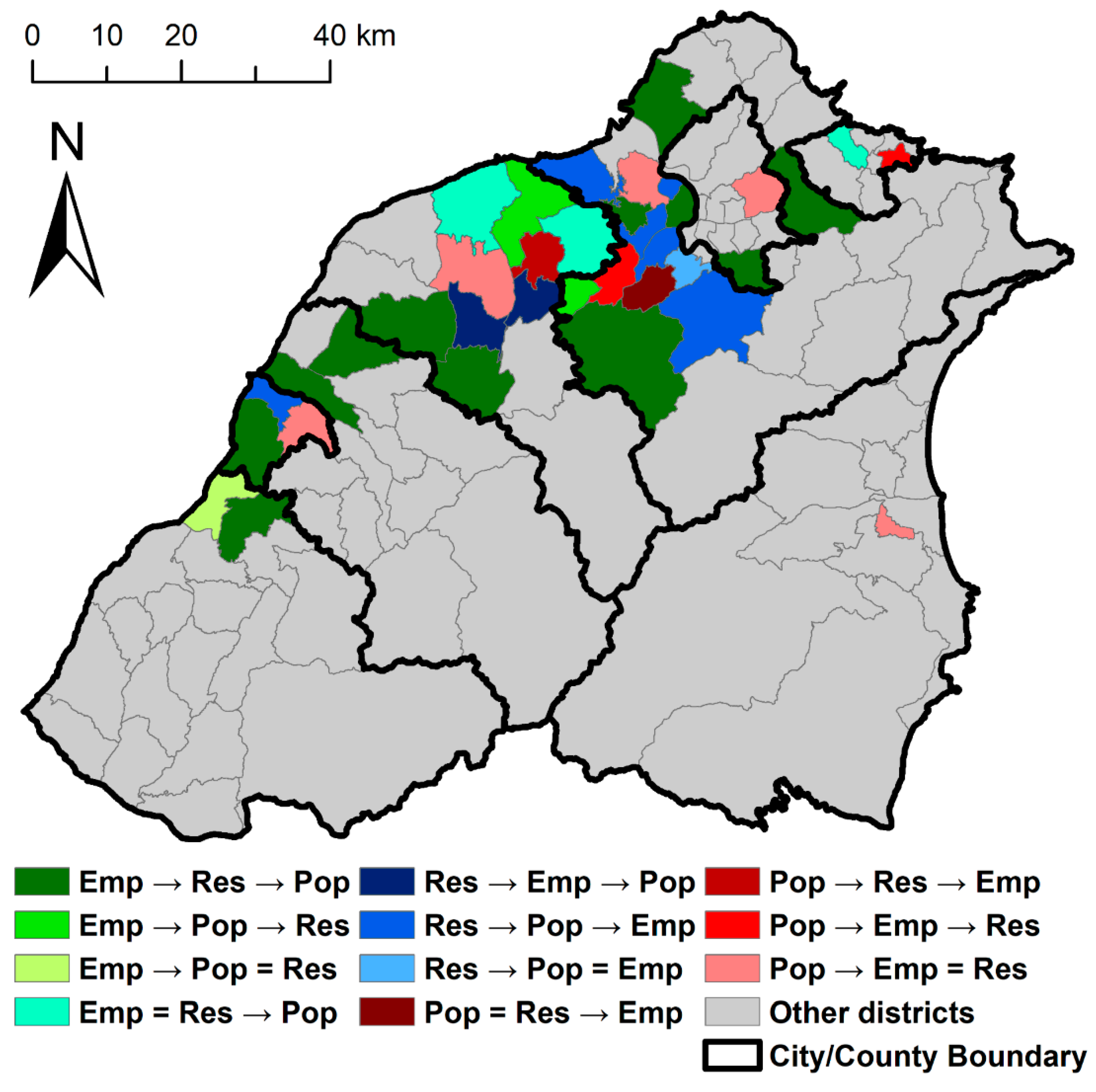
To test the hypothesis that Employment land use expanded, followed by Residential expansion, and then population growth, the relative timing among population growth, Residential, and Employment expansion was examined by the time lags of population-Residential and population-Employment. According to Table 5, the general change sequence can be based on the median of time lags among the three variables over the 36 districts. According to the median of time lags, the general progression was Employment expansion occurring first, followed by Residential expansion, and then population growth at the end, which matches our hypothesis.
The specific change sequences for the 36 districts are mapped in Figure 8. Twelve of the 36 districts matched the change sequence of Employment-Residential-population, two matched the change sequence of Employment-population-Residential, while other districts exhibited other sequences. We found that the cores of metropolitan areas tended to exhibit population growth prior to land use change (i.e., the districts showing in reddish hues). On the other hand, districts in the periphery of the metropolitan areas exhibited Employment and Residential expansion prior to population change (i.e., the districts showing green and blue hues).
Our explanation for why some districts with population growth experienced different change sequences other than those we proposed is that cores of metropolitan areas provide more jobs than the periphery and other agriculture-based districts. People crowded into the core area as renters even though available residential spaces did not meet the rental demand. Residential expanded slowly in the core areas owing to high land prices and limited undeveloped space. Construction companies perceived the need for residential spaces in the core areas, and developed new residential areas in the periphery, where land prices were lower, before the added population arrived. Although people moved into the periphery after residential construction was completed, they still commuted to the core areas for work. Therefore, the spatial connection between the core and periphery of metropolitan areas should be considered along with the hypothesis we proposed.
5. Discussion and Conclusions
5.1. Discussion
Population growth stemming from net migration was confirmed by evaluating the temporal trend of natural increase and net migration, and the associated urban land expansion was confirmed to be partially resulting from net migration. Net migration has been suggested as a source of growing population pressure in urban areas, and influence urban expansion, but the magnitude has been rarely reported (e.g., [7,8,13,22]). Here, we observe that net migration accounts for 30% of the population growth at the City/County level, and future studies should focus on upscaling net migration from city/county to district levels for estimating the direct impacts from net migration.
The relationship between population and urban areal coverage was reported in a few studies, and such relationships are linear and moderate within these study areas. For Brazil, the relationship was found to be strong when a logarithm transformation was applied (R2 = 0.9; [12]). A linear relationship was found within southeast Ghana (R2 = 0.79), which implies that urban areal coverage highly reflects on the district population count [13]. However, the relationship between population density (normalized population in our case) and urban land coverage is similar to the results that were found for southeast Ghana. More future studies should isolate population and population density from other independent variables to systematically compare such relationship in other cities and regions.
The relative timing between population change and land use change is affected by the modifiable areal unit problem (MAUP). The lag correlation was applied at the city and district scale, and Hsinchu City was used as an example (shown in Table 6). Different time lags were found in the urban core areas and the entire city, and the differences due to MAUP should be explored in future studies. However, aggregation from district to city level is inappropriate for cities with large coverage (e.g., New Taipei City and Taoyuan City) because population growth in a district hardly drives or is driven by land use change in other distant districts within the same city. Thus, time lags derived from the aggregated level data can be erroneous for such large cities. In this study, we confirm that the relationship between population and environments is not unidirectional, but rather reciprocal [11]. Within the context of urbanization, the change sequence between population and land use change varies depending on the relative location to the urban core areas. Districts in the urban core areas (e.g., districts in west of Taipei City) experienced depopulation while the land use stays the same. On the other hand, districts located in the suburban and peri-urban areas tend to have Residential and Employment expansion prior to population growth. Antrop examined Europe cities with four stages of urbanization in terms of population size, including urbanization, suburbanization, disurbanization, and reurbanization [22]. Depopulation occurred in the districts’ urban core of Taipei City, while population substantially increased in the urban core of Taoyuan City (shown in Figure 4A). Difference in population change reflects on different urbanization stages: disurbanization for Taipei City, while urbanization for Taoyuan City. Future study can focus on the entire time series of population and urban land use dynamics to better examine the urbanization stages and reciprocal relationship.
Two limitations may have influenced the results of this study. Differences between the people enumerated in the population register and the census exist, and the actual population for districts in urban areas is underestimated while overestimated for rural districts. No existing district-level data can be applied to adjust such misestimation in population count. Thus, the resultant time lag between population growth and residential expansion could partially reflect the latency of the population register system. The approaches we used to derive annual land use data were designed within the context of urban expansion, and we assumed that no changes occurred within developed areas. Later, we found evidence of urban renewal and park conversion. To accurately account for urban land use areal coverage over space and time, more research effort should be put on generation of land use time series.
The estimated relative timing between population change and land use change is restricted to the study period for which we have data. The entire trajectories of population and land use were not recorded in the data for some developed districts, and the initial statuses of population and land use remain unknown for these data. Thus, time lags that we estimated through lagged correlation could be mis-specified. Therefore, more case studies should be conducted with the same approaches with a longer study period to reconfirm our findings and test our hypothesis of urbanization processes.
Mobile phone signal data with geographical coordinates could provide a data source for augmenting satellite-derived mapping of land use [29] and population estimates [30]. Toole et al. derived weekday-weekend human activity schedules from individual-based time series mobile phone data, and then inferred land use types based on the weekday-weekend daily activity schedules [29]. Deville et al. estimated population density based on mobile phone signals at fine spatial (cellular tower zone) and temporal (seasonal) levels [30]. The resultant land-use map and population estimates were found to be accurate and precise.
5.2. Conclusions
This is the first study to examine the relative timing between population change and land-use change and to identify the cause–effect relationships based on fine spatial and temporal scale of population and land-use data at the annual time scale. This was possible because of the unique availability of annual population data for Taiwan, and the readily accessible and free long-term archive of Landsat surface reflectance data.
Linear regression models were run for each type of land use versus population to understand the general relationship between the abundance of land use and population. We found that the areal extent of Residential land use (and change) was most related to population count (and change), and the relationship was stronger when Residential and population were normalized by district areas. Future studies should put effort into separating residential land from the remainder of urban land use for estimating the impacts from population growth in other cities.
The relative timing between population growth and land use change was estimated with lagged correlation. Population growth generally occurred 2.5 years later than Residential land expansion based on the median time lag, and most districts experienced population growth later than Residential land expansion. With the lagged correlation test results, the hypothetical change sequence of population growth and land use expansion was validated within the context of urbanization. Fourteen districts with population growth exhibited our hypothetical change sequence of population growth and land-use expansion. Other districts exhibited different change sequences, primarily due to the closeness of metropolitan cores that provide abundant jobs.
Finally, the expansion of Residential and Employment land uses was deemed to be an important driver of population change. Synchronized OLS, time lag OLS, synchronized GWR, and time lag GWR were applied to model population change with the Residential and Employment change as predictors. Population change modeled with GWR, along with time lags of Residential and Employment change, were found to have the highest adjusted R2-values. We confirm the reciprocal relationship between population and environment (land use in our case) instead of a unidirectional impact from population to land use.
Author Contributions
Conceptualization, H.-C.S., D.A.S. and J.R.W.; methodology, H.-C.S., J.R.W., K.G.G. and L.M.V.C.; software, H.-C.S.; validation, H.-C.S.; formal analysis, H.-C.S.; investigation, H.-C.S.; resources, H.-C.S.; data curation, H.-C.S.; writing—original draft preparation, H.-C.S.; writing—review and editing H.-C.S., D.A.S., J.R.W., K.G.G. and L.M.V.C.; visualization, H.-C.S.; supervision, D.A.S.; project administration, H.-C.S.; funding acquisition, H.-C.S. and D.A.S. All authors have read and agreed to the published version of the manuscript.
Funding
This study was funded by Yin Chin Foundation from the USA, STUF United Fund Inc., the Long Jen-Yi Travel fund, the William and Vivian Finch Scholarship, and a doctoral stipend through San Diego State University.
Institutional Review Board Statement
Not applicable.
Informed Consent Statement
Not applicable.
Data Availability Statement
The data presented in this study are openly available in FigShare at https://doi.org/10.6084/m9.figshare.14888988.
Acknowledgments
We acknowledge suggestion from three anonymous reviewers and the journal editor.
Conflicts of Interest
The authors declare no conflict of interest.
References
- Seto, K.C.; Fragkias, M.; Güneralp, B.; Reilly, M.K. A Meta-Analysis of Global Urban Land Expansion. PLoS ONE 2011, 6, e23777. [Google Scholar] [CrossRef] [PubMed]
- United Nations. Sustainable Cities, Human Mobility and International Migration: Report of the Secretary-General; United Nations: New York, NY, USA, 2018. [Google Scholar]
- Zhao, M.; Cheng, C.; Zhou, Y.; Li, X.; Shen, S.; Song, C. A global dataset of annual urban extents (1992–2020) from harmonized nighttime lights. Earth Syst. Sci. Data 2022, 14, 517–534. [Google Scholar] [CrossRef]
- Adam, D. World population hits eight billion—here’s how researchers predict it will grow. Nature 2022. [Google Scholar] [CrossRef] [PubMed]
- Bhatta, B. Analysis of Urban Growth and Sprawl from Remote Sensing Data; Springer: Berlin, Germany, 2010; pp. 17–36. [Google Scholar]
- Reilly, M.K.; O’Mara, M.P.; Seto, K.C. From Bangalore to the Bay Area: Comparing transportation and activity accessibility as drivers of urban growth. Landsc. Urban Plan. 2009, 92, 24–33. [Google Scholar] [CrossRef]
- Wu, R.; Li, Z.; Wang, S. The varying driving forces of urban land expansion in China: Insights from a spatial-temporal analysis. Sci. Total Environ. 2020, 766, 142591. [Google Scholar] [CrossRef]
- Li, G.; Sun, S.; Fang, C. The varying driving forces of urban expansion in China: Insights from a spatial-temporal analysis. Landsc. Urban Plan. 2018, 174, 63–77. [Google Scholar] [CrossRef]
- Mahtta, R.; Fragkias, M.; Güneralp, B.; Mahendra, A.; Reba, M.; Wentz, E.A.; Seto, K.C. Urban land expansion: The role of population and economic growth for 300+ cities. NPJ Urban Sustain. 2022, 2, 5. [Google Scholar] [CrossRef]
- Lambin, E.F.; Turner, B.L.; Geist, H.J.; Agbola, S.B.; Angelsen, A.; Bruce, J.W.; Coomes, O.T.; Dirzo, R.; Fischer, G.; Folke, C.; et al. The causes of land-use and land-cover change: Moving beyond the myths. Glob. Environ. Change 2001, 11, 261–269. [Google Scholar] [CrossRef]
- de Sherbinin, A.; Carr, D.; Cassels, S.; Jiang, L. Population and Environment. Annu. Rev. Environ. Resour. 2007, 32, 345–373. [Google Scholar] [CrossRef]
- Powell, R.L.; Roberts, D.A. Characterizing Variability of the Urban Physical Environment for a Suite of Cities in Rondônia, Brazil. Earth Interact. 2008, 12, 1–32. [Google Scholar] [CrossRef]
- Stow, D.A.; Weeks, J.R.; Shih, H.-C.; Coulter, L.L.; Johnson, H.; Tsai, Y.-H.; Kerr, A.; Benza, M.; Mensah, F. Inter-regional pattern of urbanization in southern Ghana in the first decade of the new millennium. Appl. Geogr. 2016, 71, 32–43. [Google Scholar] [CrossRef] [Green Version]
- Miyauchi, T.; Setoguchi, T.; Ito, T. Quantitative estimation method for urban areas to develop compact cities in view of unprecedented population decline. Cities 2021, 114, 103151. [Google Scholar] [CrossRef]
- Scheuer, S.; Haase, D.; Volk, M. On the Nexus of the Spatial Dynamics of Global Urbanization and the Age of the City. PLoS ONE 2016, 11, e0160471. [Google Scholar] [CrossRef] [PubMed]
- Weeks, J.R. Defining Urban Areas. In Remote Sensing of Urban and Suburban Areas; Rashed, T., Jürgens, C., Eds.; Springer: Dordrecht, The Netherlands, 2010; Volume 10, pp. 33–45. [Google Scholar] [CrossRef]
- Clark, W.A.V. Human Migration. Reprint. Edited by Grant Ian Thrall. In WVU Reserch Report; Regional Research Institute, West Virginia University: Morgantown, WV, USA, 2020; pp. 22–36. [Google Scholar]
- Massey, D.S. Why does immigration occur? A theoretical synthesis. In The Handbook of International Migration: The American Experience; Hirschman, C., Kasinitz, P., Dewind, J., Eds.; Russell Sage Foundation: New York, NY, USA, 1999; pp. 34–52. [Google Scholar]
- Bencivenga, V.R.; Smith, B.D. Unemployment, Migration, and Growth. J. Political Econ. 1997, 105, 582–608. [Google Scholar] [CrossRef] [Green Version]
- Gubhaju, B.; De Jong, G.F. Individual versus Household Migration Decision Rules: Gender and Marital Status Differences in Intentions to Migrate in South Africa. Int. Migr. 2009, 47, 31–61. [Google Scholar] [CrossRef] [Green Version]
- Fan, C.C. Rural-urban migration and gender division of labor in transitional China. Int. J. Urban Reg. Res. 2003, 27, 24–47. [Google Scholar] [CrossRef]
- Antrop, M. Landscape change and the urbanization process in Europe. Landsc. Urban Plan. 2004, 67, 9–26. [Google Scholar] [CrossRef]
- Bell, S.; Alves, S.; De Oliveira, E.S.; Zuin, A. Migration and Land Use Change in Europe: A Review. Living Rev. Landsc. Res. 2010, 4, 1–49. [Google Scholar] [CrossRef] [Green Version]
- Shih, H.-C.; Stow, D.A.; Tsai, Y.-M.; Roberts, D.A. Estimating the starting time and identifying the type of urbanization based on dense time series of landsat-derived Vegetation-Impervious-Soil (V-I-S) maps—A case study of North Taiwan from 1990 to 2015. Int. J. Appl. Earth Obs. Geoinf. ITC J. 2019, 85, 101987. [Google Scholar] [CrossRef]
- Wu, C. Normalized spectral mixture analysis for monitoring urban composition using ETM+ imagery. Remote. Sens. Environ. 2004, 93, 480–492. [Google Scholar] [CrossRef]
- Shih, H.-C.; Stow, D.A.; Chang, K.-C.; Roberts, D.A.; Goulias, K.G. From land cover to land use: Applying random forest classifier to Landsat imagery for urban land-use change mapping. Geocarto Int. 2021, 37, 5523–5546. [Google Scholar] [CrossRef]
- Raffalovich, L.E. Detrending Time Series. Sociol. Methods Res. 1994, 22, 492–519. [Google Scholar] [CrossRef]
- Fotheringham, A.S.; Charlton, M.E.; Brunsdon, C. Geographically Weighted Regression: A Natural Evolution of the Expansion Method for Spatial Data Analysis. Environ. Plan. A Econ. Space 1998, 30, 1905–1927. [Google Scholar] [CrossRef]
- Toole, J.L.; Ulm, M.; González, M.C.; Bauer, D. Inferring land use from mobile phone activity. In Proceedings of the ACM SIGKDD International Workshop on Urban Computing, Beijing, China, 12–16 August 2012; pp. 1–8. [Google Scholar] [CrossRef]
- Deville, P.; Linard, C.; Martin, S.; Gilbert, M.; Stevens, F.R.; Gaughan, A.E.; Blondel, V.D.; Tatem, A.J. Dynamic population mapping using mobile phone data. Proc. Natl. Acad. Sci. USA 2014, 111, 15888–15893. [Google Scholar] [CrossRef]
Figure 1.
Study area for north region of Taiwan along with the cores of metropolitan areas within the study area.
Figure 1.
Study area for north region of Taiwan along with the cores of metropolitan areas within the study area.

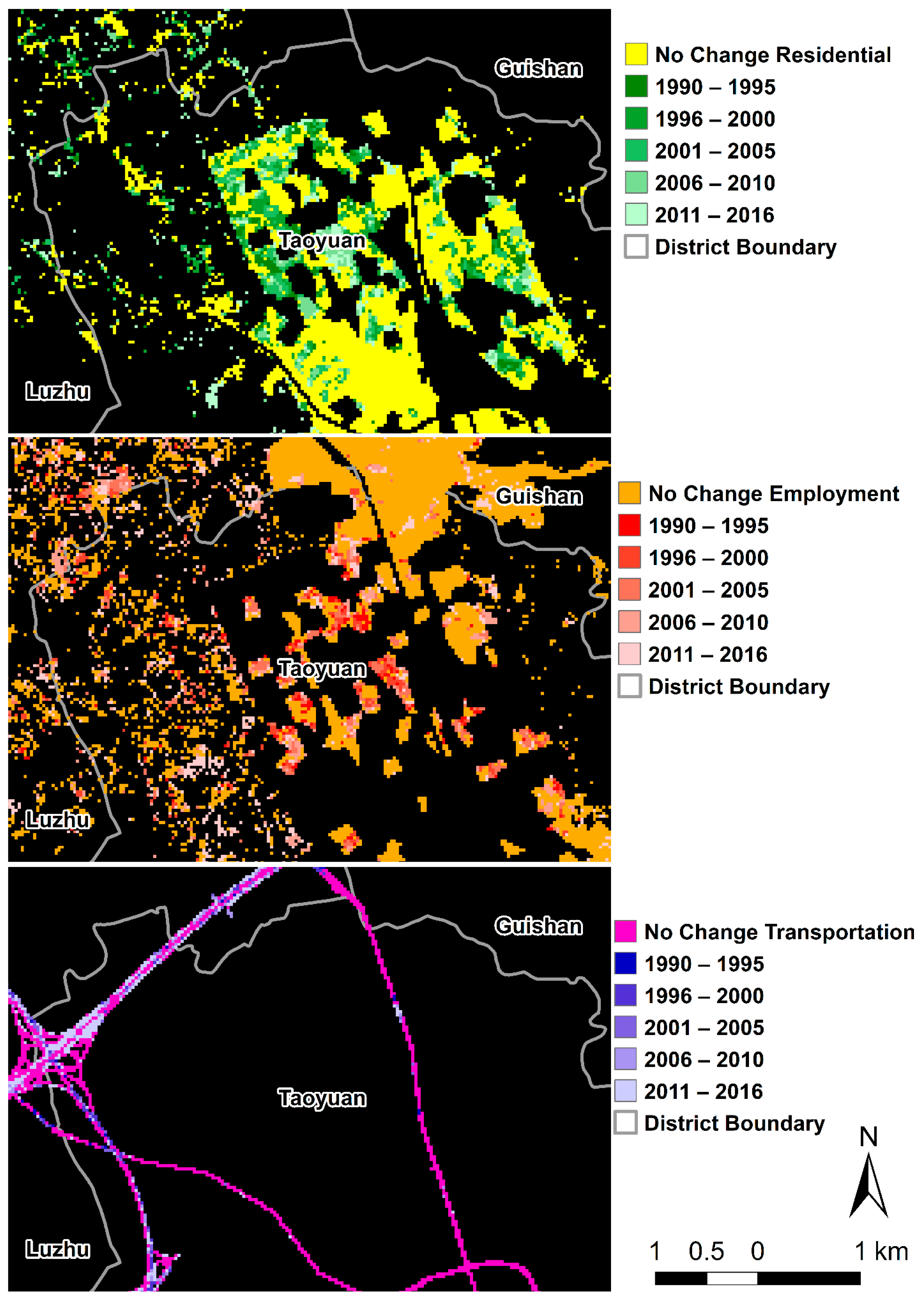
Figure 2.
Subset showing date for when urban land use change occurred between from 1990 to 2015; (top) Residential; (middle) Employment; (bottom) Transportation.
Figure 2.
Subset showing date for when urban land use change occurred between from 1990 to 2015; (top) Residential; (middle) Employment; (bottom) Transportation.

Figure 3.
Temporal population dynamics for cities/counties with population data from registers and censuses. (a) shows the population count in the three census years. Cities and counties with more in-migrants had more people counted in the census than were registered as living there, while the remainder of counties experienced out-migration. (b) shows the annual natural increase (N) and net migration (M) data at the City/County level published by the registered population system.

Figure 4.
Equal interval choropleth maps of population count and land use (Residential, Employment, and Transportation) change (in % of district size) from 1991 to 2015. (A) population count change; (B) residential land use change; (C) employment land use change; and (D) transportation land use change.

Figure 5.
R2 between population and land use and their changes. The legend shows the corresponding land use, and population is the independent variable for all linear regression. Normalized refers to both population and the land use being normalized by the size of districts. The x-axes of (B–D) show the end year of the time interval. (A) annual population and land use; (B) annual change of population and land use; (C) 5-year change of population and land use; (D) 10-year change of population and land use. R2-values derived from population, land use area, and their changes were derived from the same year or same period without time lag.

Figure 6.
Maps depicting time lag (in years) between population growth and land use expansion by district. (A) Residential land use; (B) Employment land use; (C) Transportation corridor; and (D) General Urban (the sum of three land use types). Positive signs of time lags indicate that population growth occurred later than land use expansion, while the negative signs indicate that population growth occurred earlier than land use expansion.

Figure 7.
Equal interval choropleth maps of local R2 and coefficients derived from geographically weighted regression for modeling population change from 2005 to 2015 with Residential change from 2002 to 2012 and Employment change from 2001 to 2011. (A) local R2; (B) coefficients of local intercept; (C) coefficients of local Residential change; (D) coefficients of local Employment change.

Figure 8.
Map of change sequence among population (Pop), Residential (Res), and Employment (Emp) for the 36 districts with greatest population change or population density change. “→” indicates one occurred prior to the other. For example, Emp → Res refers that employment expansion occurred prior to Residential. “=” indicates one occurred at the time of the other. For example, Emp = Res indicates Employment and Residential expansion occurred at the same time.


Table 1.
Data summary.
| Data Type | Data Source | Spatial Granularity | Temporal Coverage |
|---|---|---|---|
| Digital geographic information system file | District polygon shapefile | District | N/A |
| Population | Census population count | County | 1990, 2000, 2010 |
| Registered population count | District | 1991 to 2015 | |
| Registered natural increase | County | 1992 to 2015 | |
| Registered net migration | County | 1992 to 2015 | |
| Land use | Urban expansion time map derived from Landsat time series | 30 by 30 m pixel (areal coverage aggregated to district) | 1990 to 2015 |
| 2015 Land use map derived from Landsat 8 OLI imagery | 30 by 30 m pixel (areal coverage aggregated to district) | 2015 |
Table 2.
User’s and producer’s accuracy of land use change map.
| No Change | Change | ||||||
|---|---|---|---|---|---|---|---|
| Other | Transportation | Employment | Residential | Transportation | Employment | Residential | |
| User’s accuracy | 95.6 | 87.0 | 75.6 | 70.6 | 41.6 | 69.5 | 81.8 |
| Producer’s accuracy | 91.6 | 62.1 | 77.0 | 90.0 | 31.2 | 73.3 | 60.0 |
Table 3.
Descriptive statistics of registered population, population density, and population change at the district level.
Table 3.
Descriptive statistics of registered population, population density, and population change at the district level.
| District Area (km2) | Population Count 1991 | Population Count 2015 | Population Count Change | Population Density 1991 (pop/km2) | Population Density 2015 (pop/km2) | Population Density Change (pop/km2) | |
|---|---|---|---|---|---|---|---|
| Maximum | 769.9 | 542,942 | 554,236 | 181,089 | 40,190.7 | 36,607.7 | 11,345.2 |
| Mean | 86.4 | 86,723 | 104,219 | 17,495 | 4369.1 | 4699.6 | 330.5 |
| Median | 54.2 | 49,581 | 53,634 | 2725 | 745.1 | 1124.5 | 53.9 |
| Minimum | 4.5 | 3247 | 4606 | −39,049 | 6.9 | 7.8 | −4884.1 |
| Standard Deviation | 125.6 | 100,481 | 114,591 | 35,337 | 8142.7 | 7846.3 | 1724.7 |
Change is the difference between 1991 to 2015.
Table 4.
Statistics of Residential, Employment, and Transportation over districts.
| Res 1991 (%) | Res 2015 (%) | Res Change (%) | Emp 1991 (%) | Emp 2015 (%) | Emp Change (%) | Tra 1991 (%) | Tra 2015 (%) | Tra Change (%) | |
|---|---|---|---|---|---|---|---|---|---|
| Maximum | 53.0 | 55.6 | 8.9 | 34.2 | 37.7 | 10.1 | 15.8 | 15.9 | 1.7 |
| Mean | 9.2 | 10.9 | 1.6 | 8.2 | 10.5 | 2.2 | 3.1 | 3.6 | 0.4 |
| Median | 4.2 | 5.2 | 0.8 | 6.1 | 7.4 | 0.9 | 2.5 | 3.1 | 0.3 |
| Minimum | 0.1 | 0.1 | 0.0 | 0.0 | 0.0 | 0.0 | 0.0 | 0.0 | 0.0 |
| Standard Deviation | 11.5 | 12.3 | 1.7 | 7.4 | 9.2 | 2.7 | 2.9 | 3.0 | 0.4 |
Res = Residential; Emp = Employment; Tra = Transportation. Change is the difference between 1991 and 2015. % indicates the percent coverage of district area.
Table 5.
Time lag (in years) between population and land use identified by max lag correlation.
| Residential | Employment | Transportation | Urban | |
|---|---|---|---|---|
| Mean | 1.5 | 1.3 | −0.1 | 1.0 |
| Standard deviation | 6.7 | 7.8 | 7.1 | 7.8 |
| Minimum | −10 | −10 | −10 | −10 |
| 25% quantile | −2 | −6.5 | −6 | −8 |
| median | 2.5 | 3.5 | −1.5 | 2.5 |
| 75% quantile | 6 | 9 | 8 | 9 |
| Maximum | 10 | 10 | 10 | 10 |
Positive sign of time lag indicates that population growth occurred later than land use change, while the negative sign of time lag indicates that population growth occurred earlier than land use change.
Table 6.
Time lags (in years) for Hsinchu City and its associated district.
| Residential | Employment | Transportation | Urban | |
|---|---|---|---|---|
| Hsinchu City | 9 | 9 | 9 | 9 |
| East district | −10 | −10 | 10 | −10 |
| North district | 6 | 6 | −7 | 8 |
| XiangShan district | 3 | 9 | 8 | 9 |
Table 7.
Adjusted R2 of 10-year interval change in population and land use.
| Year | Synchronized OLS | Time Lag OLS | Synchronized GWR | Time Lag GWR |
|---|---|---|---|---|
| 2001 | 0.45 | - | 0.60 | - |
| 2002 | 0.44 | - | 0.59 | - |
| 2003 | 0.46 | - | 0.61 | - |
| 2004 | 0.49 | - | 0.67 | - |
| 2005 | 0.52 | 0.55 | 0.69 | 0.72 |
| 2006 | 0.52 | 0.57 | 0.68 | 0.76 |
| 2007 | 0.53 | 0.60 | 0.68 | 0.76 |
| 2008 | 0.54 | 0.60 | 0.84 | 0.79 |
| 2009 | 0.53 | 0.60 | 0.73 | 0.79 |
| 2010 | 0.55 | 0.61 | 0.66 | 0.78 |
| 2011 | 0.53 | 0.60 | 0.67 | 0.73 |
| 2012 | 0.49 | 0.58 | 0.66 | 0.72 |
| 2013 | 0.45 | 0.57 | 0.65 | 0.73 |
| 2014 | 0.41 | 0.54 | 0.65 | 0.78 |
| 2015 | 0.41 | 0.54 | 0.65 | 0.73 |
Publisher’s Note: MDPI stays neutral with regard to jurisdictional claims in published maps and institutional affiliations. |
© 2022 by the authors. Licensee MDPI, Basel, Switzerland. This article is an open access article distributed under the terms and conditions of the Creative Commons Attribution (CC BY) license (https://creativecommons.org/licenses/by/4.0/).
Share and Cite
MDPI and ACS Style
Shih, H.-C.; Stow, D.A.; Weeks, J.R.; Goulias, K.G.; Carvalho, L.M.V. The Relative Timing of Population Growth and Land Use Change—A Case Study of North Taiwan from 1990 to 2015. Land 2022, 11, 2204. https://doi.org/10.3390/land11122204
AMA Style
Shih H-C, Stow DA, Weeks JR, Goulias KG, Carvalho LMV. The Relative Timing of Population Growth and Land Use Change—A Case Study of North Taiwan from 1990 to 2015. Land. 2022; 11(12):2204. https://doi.org/10.3390/land11122204
Chicago/Turabian StyleShih, Hsiao-Chien, Douglas A. Stow, John R. Weeks, Konstadinos G. Goulias, and Leila M. V. Carvalho. 2022. "The Relative Timing of Population Growth and Land Use Change—A Case Study of North Taiwan from 1990 to 2015" Land 11, no. 12: 2204. https://doi.org/10.3390/land11122204
Note that from the first issue of 2016, this journal uses article numbers instead of page numbers. See further details here.