Construction of Urban Green Space Network in Kashgar City, China

Abstract

With the new round of western development being pushed forward and territorial spatial planning being put into place, northwest China’s urbanization rate has sped up. Urbanization will inevitably affect the city’s general landscape pattern and features, aggravating the landscape’s fragmentation and destroying the urban ecological environment. That threatens the well-being of the residents and the city’s biodiversity. Urban green space provides a habitat for the creatures in the city, and its connectivity provides corridors. Researchers and planners have developed green space networks to protect urban biodiversity and satisfy urban residents’ needs for recreation and ecologically friendly open space. This study uses RS, GIS, SeNtinel Application Platform (SNAP), and Conefor Sensinode. Applying the landscape connectivity index, least-cost path model, and corridor curvature analysis to identify potential recreation and biodiversity conservation corridors with a reasonable width, identifies good quality green space patches and corridors, or which ones need improvement. The results show that: (1) The patches selected by the possible connectivity index (PC) calculated with a threshold of 100 m in the urban area of Kashgar have higher recreational attributes. (2) There are 24 effective recreational corridors in Kashgar, with a total length of 43.44 km, and 53 effective biodiversity conservation corridors, a total of 78.23 km. Suppose recreational and ecological functions are considered to build a comprehensive green space network. The 50 m recreational corridor is mainly distributed in the center, and the 30 m biodiversity conservation corridor is primarily distributed on edge. (3) We can determine the location of the new green space suitable for protection or development by analyzing the corridor curvature. Through the constructed green space network, we can find that green space planning has severe fragmentation, unfair distribution, and other problems. Based on these issues, optimizing urban green space can promote the connectivity of urban green space. Furthermore, studying the width of corridors suitable for dense urban areas is conducive to protecting urban biodiversity and resident well-being.

1. Introduction

A growing body of research shows that urban green spaces provide important spiritual, recreational, and cultural services that improve the health of residents [1,2,3,4]. Urban green space has a positive effect on both physical and mental health. Physical health benefits include improved birth outcomes, a decrease in cancer incidence and morbidity, and a decrease in cardiovascular disease incidence [5,6,7]; mental health benefits include improved attention, mood, depression, and stress management [5,8]. Furthermore, urban green spaces promote leisure and physical activity while improving social interaction [9].

Urban green spaces are the second-largest biological component in cities after residents. It is a semi-natural city area that accommodates a wide variety of plant communities and small animals with a wide range of environmental benefits and ecological functions. Studies have shown that green spaces can regulate carbon and water cycles [10], prevent soil erosion, regulate temperature, and purify the air. For example, urban trees reduce pollutant emissions by lowering air temperatures or reducing energy consumption in buildings [11]. Additionally, urban green spaces are important for biodiversity conservation [12], while urban green spaces that are abundant in biodiversity improve people’s quality of life and promote sustainable lifestyles [4].

Rapid urbanization and population increase have caused extinction crises, changing the focus of natural protection from the preservation of specific sites to the preservation of networks of green spaces that include more landscapes [13]. The green space network is made up of various types of nodes and corridors [14], combining different social, economic, cultural, and other functions [15] to address increased land use and fragmentation and to protect the connectivity of threatened natural species and habitats [16]. Green space networks are often referred to as green infrastructure networks or green space ecological networks [14,17]. The open spaces that connect parks, nature reserves, cultural landscapes, and their communities are referred to as ecological networks by Little in “Greenways for America” [18]. No matter their size, composition, or use, Tzoulas et al. define urban green space networks as informal natural places related in shape or function [19].

The principles of landscape ecology are widely used in urban green space planning to guide green space networks at different levels in regions, cities, and communities [20,21,22], laying the foundation for developing urban green space network models for research. Kong et al. pioneered an urban green space network model using the least-cost path method to identify potential corridors in Jinan and developed and improved a green space network based on Graph Theory and Gravity Model for biodiversity conservation. In addition, they used land use type as the basis for resistance allocation by selecting cores based primarily on the patch size [14,23]. Wu et al. constructed a network of green spaces through the landscape connectivity index and the least-cost path method supported by RS and GIS technology. They then used the corridor curvature index to identify corridors that needed additional optimization [24]. Some scholars have also addressed the ecological source problem by using morphological spatial pattern analysis and ecological connectivity index analysis methods to construct an ecological network system of green spaces in the study area based on the landscape pattern of green spaces in the study area [25]. Mougiakou et al. argued that connectivity plays an important role in controlling and assessing the structure of generative networks. They established a generic methodological framework to evaluate and optimize urban greening networks in dense urban areas [26]. In summary, selecting green space patch nodes, creating the cost surface, and identifying the green space corridors are all essential to construct an urban green space network. The selection of green space patch nodes typically considers green space area and species richness [27], landscape connectivity [14,24,28], morphological characteristics, and spatial distribution [29,30,31]. The proper resistance factor is normally determined by the field circumstances of the study area before creating a cost surface. According to certain studies [32], cost surfaces are produced based on factors like land cover, height, slope, and population density. Several research surfaces [33,34] have been created by assigning values to factors such as land cover and landscape type. The least-cost path model is frequently used to identify corridors [35,36,37]. Concerning the spatial scale of the green space network, studies have been conducted at a variety of spatial scales, including the city [38], central city [39], and watershed [34]. In addition, studies have shown that building a network of green spaces can manage stormwater [40], optimize the layout of green infrastructure [41] and harmonize cities with nature [42].

Currently, urban green space network models are maturing. Still, we find that most studies focus more on the ecological functions of urban green space networks and neglect the recreational functions, and these studies only choose the best paths and ignore the corridor width [14,24,37]. As a result, this paper seeks to identify, through buffer zone analysis, corridors with a width appropriate for urban areas that support the survival of birds and the flow of other bioenergy in the city [43] while also being suitable for green open space for people to walk and exercise [44]. Furthermore, we found that no one has analyzed the development of urban green space networks in arid areas. A network of green spaces can assist in managing the climate in arid regions while also saving water because dry places are more water-scarce [10]. Due to this, we decided to build an urban green space network in Kashgar City, a fast-growing special economic zone in northwest China’s arid region. The main goals of this study are to (1) identify green patch nodes in Kashgar City through connectivity and green area; (2) use two groups of green space patch nodes to construct two green space networks with different main functions using the least-cost path model; (3) construct a comprehensive network of green space with reasonable corridor width; and (4) identify green space patches and corridors that need protection, optimization and development. Additionally, our study findings can serve as a guide for optimizing Kashgar’s urban green space, which will be crucial in fostering the city’s sustainable growth, safeguarding its biodiversity, and satisfying its inhabitants’ needs for green space.

2. Materials and Methods

2.1. Study Area

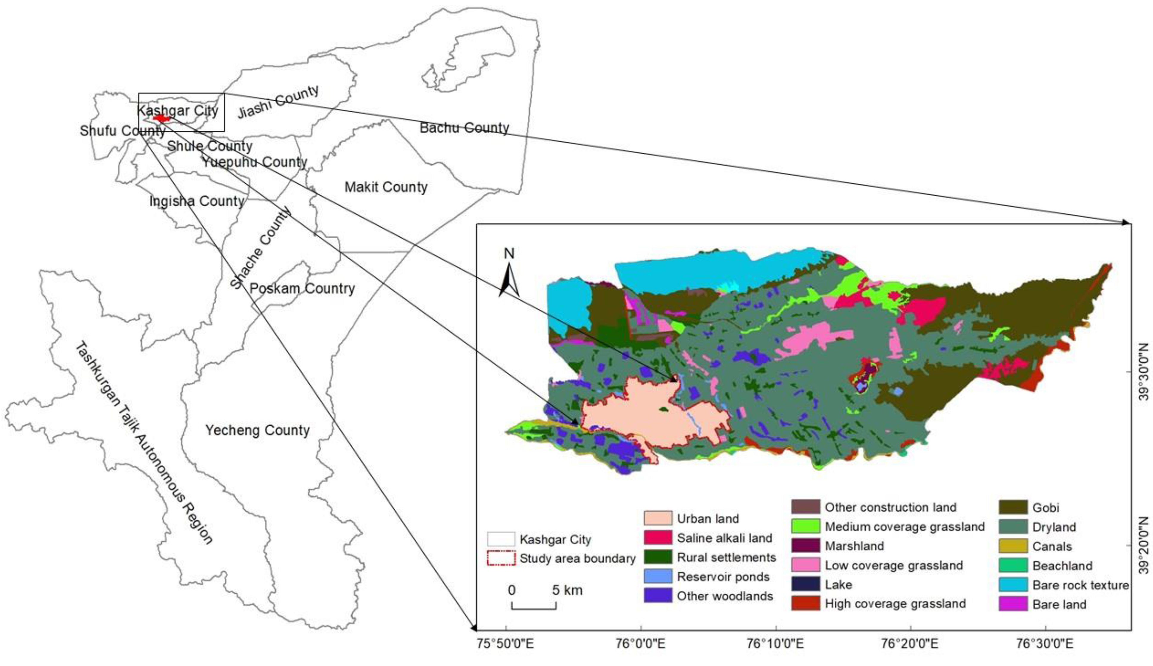
Kashgar City is located in southwest Xinjiang, between 75°50′ and 76°35′ East and 39°24′ and 39°37′ North, east of the Taklamakan Desert, south of the Karakorum Mountains and Tibet’s Ali region, and west of the Pamir Plateau. Kashgar City has a warm, continental, and arid climate with high elevation to the north and low topography to the south. The principal rivers in the region are the Kizil, the Tuman, and the Chakmak. Kashgar is located in the arid region of the northwest, where water resources are scarce, and the ecological environment is relatively fragile. National and local investment have steadily increased since the Kashgar Special Economic Zone was established in May 2010, and the population has expanded by 41.9%, from 470,000 in 2010 to 667,000 in 2020. The administrative area has expanded from 555 square kilometers in 2010 to 1059 square kilometers in 2020. Local general public budget expenditure increased by 2.21 times. The city of Kashgar has experienced rapid urbanization and significant urban spatial expansion.

This study focuses on the central area of Kashgar City, where the scope of urban construction land in Kashgar in 2020 will be 71.8 square kilometers (6.8% of Kashgar’s total area). It includes Yawag street, Chamalbagh town, Gustangboi street, Chasa street, Seman township, Pahatakri township, Nazeerbagh township, Kumudelwaza street, Haohan township, and Doraitbagh township (Figure 1).

2.2. Data Sources

Our study used data from the ESA Copernicus Data Centre (https://scihub.copernicus.eu, accessed on 21 February 2022) to obtain Sentinel-2 remote sensing imagery of L2A-class products with a spatial resolution of 10 m and 1.6% cloudiness. Kashgar City’s urban land boundary was determined using the second kind of 2020 land use remote sensing monitoring data (urban land) from the Resource and Environment Science and Data Center of the Chinese Academy of Sciences (http://www.resdc.cn, accessed on 7 March 2022). The complete accuracy of the secondary-kind classification was higher than 91.2% [45,46], which met the investigation’s standards for accuracy. We collected socioeconomic data from the China County Statistical Yearbook (County and Cities Volume) (2011–2021) (http://www.stats.gov.cn, accessed on 2 October 2022).

2.3. Methods

2.3.1. Extraction of Green Space Patch Information

Firstly, the Sentinel-2 image L2A level product was resampled and converted to ENVI format using SNAP. Then, we imported the ENVI to obtain the study area’s land types such as urban green space, construction land, water bodies, agricultural land, and other land through supervised classification. Later, we used ArcGIS to correct the classification results based on experience through high-definition images and extract information about urban green space patches.

2.3.2. Identification of Green Space Patch Nodes

(1)

Landscape connectivity indices

In general, the landscape connectivity index is used to evaluate the patch connectivity of green space systems [47]. In this study, we used Conefor 2.6 to calculate the landscape coincidence probability (LCP), integral index of connectivity (IIC), number of links (NL), number of components (NC), area-weighted flux (AWF), probability of connectivity (PC), and the importance value of each index [48], their meanings and formulas are shown in

Table 1. Landscape Connectivity Index.

Index	Formula	Description
NC	-	A component (or connected region) is a set of nodes in which a path exists between every pair of nodes.
NL	-	Links between the habitat nodes in the landscape.
LCP	$LCP={{\displaystyle \sum _{i=1}^{NC}\left(\frac{c_i}{A_L}\right)}}^2$	Where $NC$ is the number of components in the landscape, $c_i$ is the total component attribute (sum of the attributes of all the nodes belonging to that component), and $A_L$ is the maximum landscape attribute. LCP ranges from 0 to 1, increases with improved connectivity.
IIC	$IIC=\frac{{\displaystyle \sum _{i=1}^n{\displaystyle \sum _{j=1}^n\frac{a_i{a}_j}{1+n{l}_{ij}}}}}{A_L^2}$	Where $n$ is the total number of nodes in the landscape, $a_i$ and $a_j$ are the attributes of nodes $i$ and $j$, $n{l}_{ij}$ is the number of links in the shortest path (topological distance) between patches $i$ and $j$, and $A_L$ is the maximum landscape attribute. IIC ranges from 0 to 1 and increases with improved connectivity.
AWF	$AWF={\displaystyle \sum _{i=1}^n{\displaystyle \sum _{j=1,i\ne j}^n{p}_{ij}}}\cdot a_i\cdot a_j$	Where $n$ is the total number of nodes in the landscape, $p_{ij}$ is the probability of direct dispersal between nodes $i$ and $j$, and $a_i$ and $a_j$ are the attributes of the nodes $i$ and $j$.
PC	$PC=\frac{{\displaystyle \sum _{i=1}^n{\displaystyle \sum _{j=1}^n{a}_i\cdot a_j\cdot p_{ij}^{\ast }}}}{A_L^2}$	Where $n$ is the total number of habitat nodes in the landscape, $a_i$ and $a_j$ are the attributes of nodes $i$ and $j$, $A_L$ is the maximum landscape attribute, and $p_{ij}^{*}$ is the maximum product probability of all paths between patches $i$ and $j$. PC ranges from 0 to 1 and increases with improved connectivity.

.

Then, we calculated the importance value of each index. The expression is [49]:

$$dI(\%)=\frac{I-I^{\prime }}{I}\times 100$$

(1)

where $I$ is the overall connectivity index value when all landscape nodes exist and $I^{\prime }$ is the overall index value when a single landscape node is eliminated. A higher $dI$ value suggests that this patch is more important for landscape connectivity. For specific calculations, LCP, IIC, NL, NC, AWF, and PC can be taken, respectively.

Based on the NC, we calculated a range of distance thresholds, and the Spearman rank correlation coefficient was used to select the connection index with the most stable change under each threshold within this range [50]. Under the initial distance threshold, $dI$ is a variable one; under the remaining threshold, $d{I}^{\prime }$ is variable two, and its coefficient is r_s. The greater the change in r_s, the more sensitive it is to threshold changes, making it unsuitable for use as an evaluation standard.

The coefficient of variation (CV) is used to determine the threshold where the difference in the most stable importance index levels is most pronounced and to determine the final study threshold. Its formula is [51]:

$$CV=\frac{S}{\overline{dx}}$$

(2)

where $S$ is the standard deviation of the importance value of the patch connectivity index, and $\overline{dx}$ is the mean of the importance value of the connectivity index. A more considerable $CV$ value indicates a better dispersion of the importance value of the green space patches under this threshold and a more noticeable difference in rank, making it easier to select green space patch nodes.

(2)

The size of the green patches

We regarded the top 15 patches as ecological green space patch nodes among green space patches with an area of more than 1 hm² in the study area according to the size of the area.

2.3.3. Identification of Potential Corridors

The least-cost path analysis method is derived from the cost distance model based on a rasterized landscape resistance surface. It constructs a path with a cumulative minimum cost between the movement start point (source) and the target [52]. This analysis can be used to identify habitat connections that will preserve or improve connectivity [14,24]. It can also determine the minimum cost path between ecological nodes in a network of green spaces and identify potential green space corridors [14,53]. In this paper, we determined the least cost by calculating the cumulative cost from source to destination patches based on the connectivity or patch area throughout the landscape.

Assessing habitat suitability and corridor impedance is the second step in potential corridor identification. Our study area is an urban built-up area where small animals such as birds may stay on trees or grass as they move between habitats, and residents may cool off, walk or exercise in the shade of a tree on a hot summer day. Thus we combine the land cover type and human disturbance level in the study area to describe the relative resistance values for different land types, representing how difficult it is for animals or inhabitants to move between patches [24]. After conducting the field surveys, we assigned the impedance values to each land-use type based on the available literature [14,24] and the staff members’ expert opinions (

Table 2. Land-use type classification and impedance weights for the urban green space network.

Category	Description	Range of Impedance Values
Greenland	Urban green space	10
Construction	Land used for the construction of residences, public facilities, municipal utilities, warehouses, and industrial purposes. Little or no vegetation is present, though some areas have some planted vegetation (primarily shrubs and grasses).	1000
Agriculture	Sites used to grow crops for export and for local consumption.	50
Water	Lakes, rivers, streams, and canals.	600
Other	Primarily artificial land types with negligible vegetation and strong barriers to dispersal of organisms.	700

). Then we used the cost distance tools in the ArcGIS Spatial Analyst extension to create the cost surface; and the cost path tool to determine the least-cost path from a destination point to a source. Finally, we manually eliminated repeated and redundant corridors between two patches and determined potential paths.

2.3.4. Calculation of Corridor Curvature

Curvature can be used to measure how scientific and logical the corridor is. It can also assess the corridor’s structure and the rate at which organisms and energy move or spread between patches. The larger the value, the more complex the bending degree. The formula for its calculation is as follows [24]:

$$D_q=Q/L$$

(3)

where $D_q$, $Q$, and $L$ represent the corridor’s curvature, real length, and straight-line distance from the start of the corridor to a point, respectively.

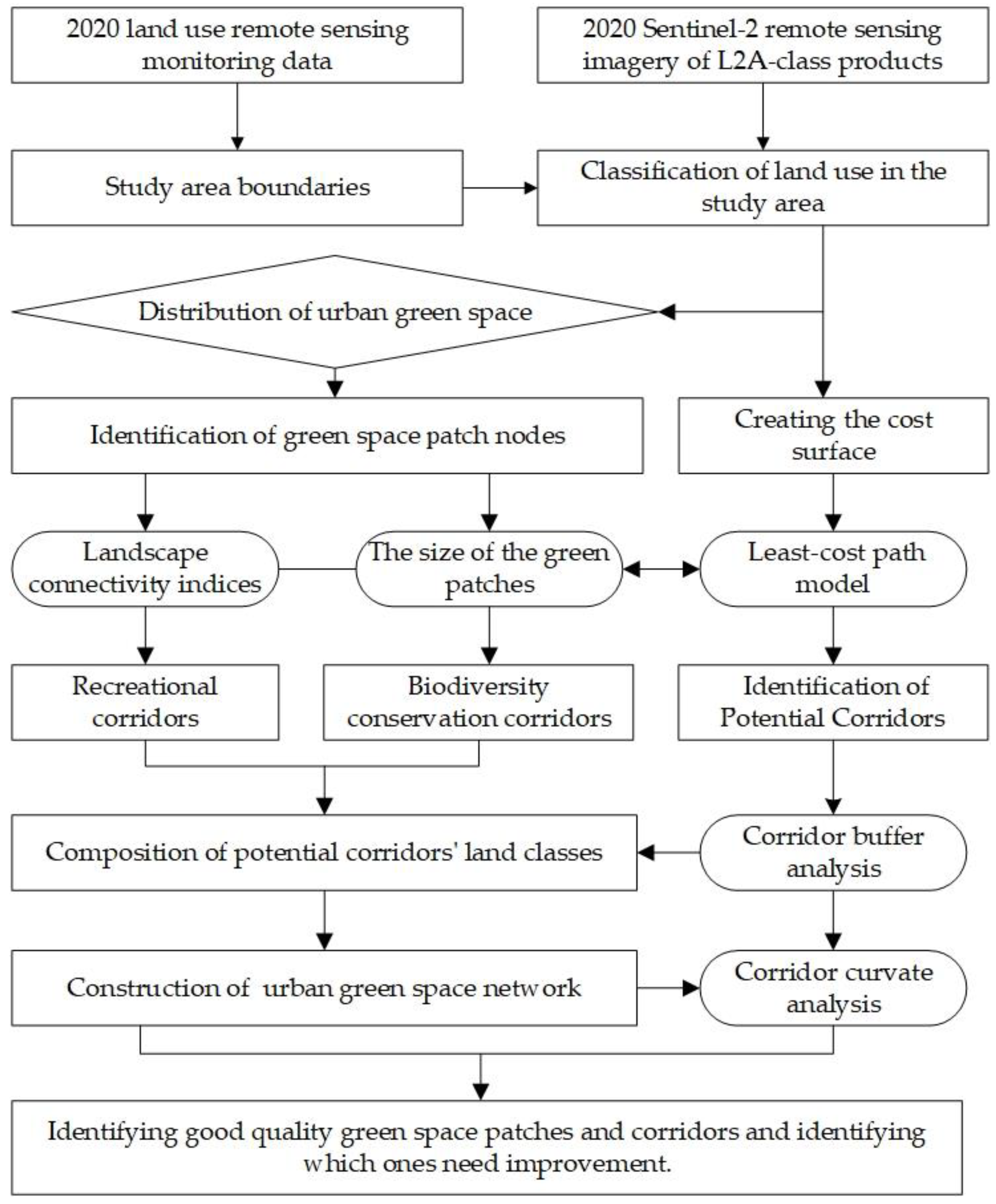
The flowchart of this research is shown in Figure 2.

3. Results

3.1. Distribution of Green Space

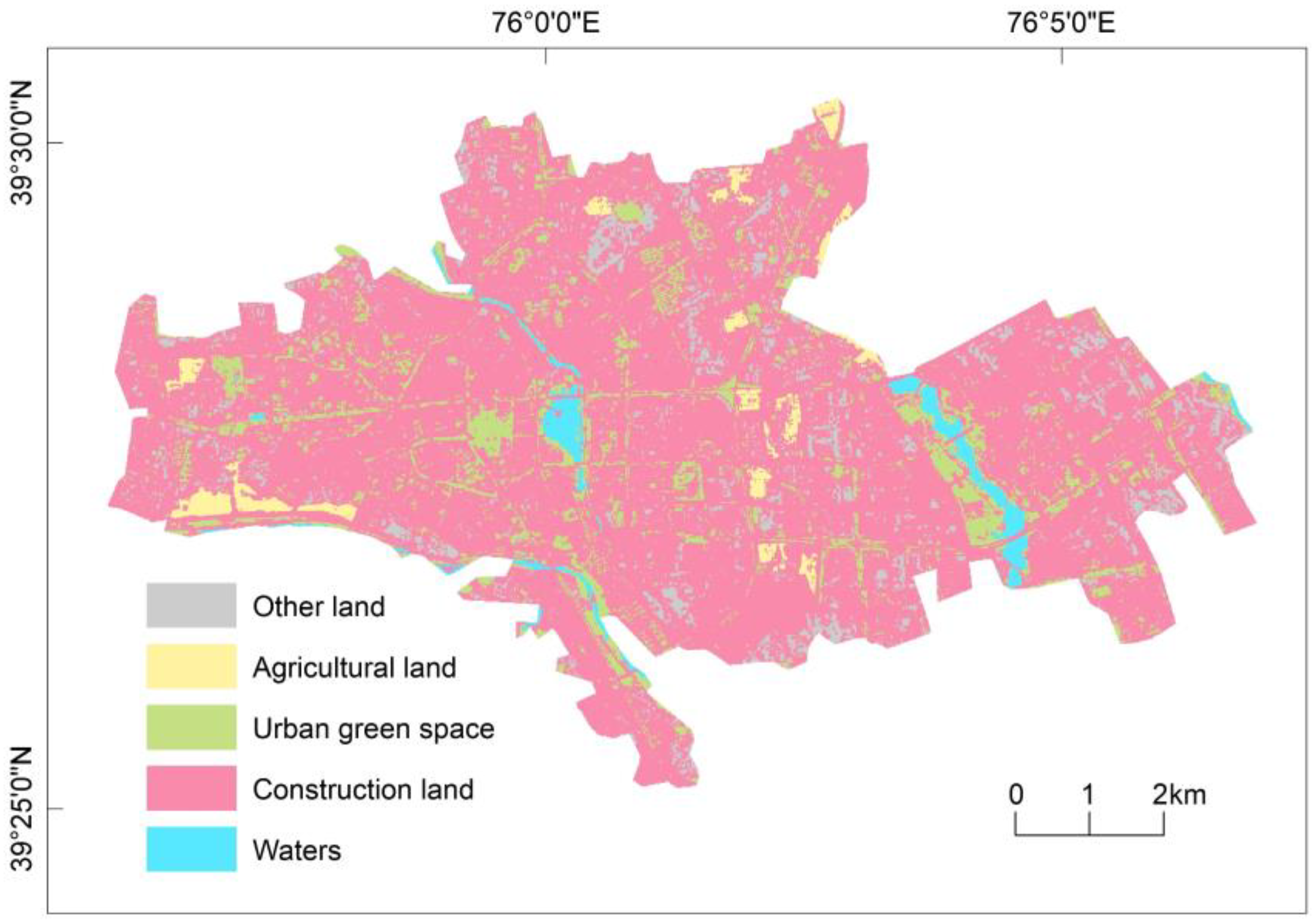
The sample test revealed that the Kappa coefficient of the land use classification results in the study region was 93.23 percent, which met the requirements of this study (Figure 3). The general area of green space patches in the study area is 767.38 hm², or 10.69 percent of the entire study area. The overall number of green space patches is 3370, representing 43.76 % of the total number of patches in the study region, indicating that the number of green space patches in the study area is high and the degree of fragmentation is high. The urban green space in the study area was categorized into five categories based on the Urban Green Space Classification Standard (CJJ/T 85-2017) and the actual situation in the study area: green park space, protective green space, square land, subsidiary green space, and regional green space [54]. Large green areas are primarily parks, including Xiaoyalang Wetland Park and Dongcheng Park in the east of the study area; People’s Park in the center; East Lake Park and South Lake Park in the middle; and West Park in the west. The little green space patches in the study area are mostly attached green spaces and protective green spaces scattered around roads and buildings on all levels.

3.2. Selection of Green Space Patches

We used the navigation map to search “Kashgar Park” after obtaining the spatial distribution of urban green space patches. Then, we chose Kashigar City parks under the “Top Parks” page as well-known green space patch nodes with high recreational service value.

The study included 147 green places with an area of more than 1 hm² each, and the NC was used to determine the connection threshold range, with the initial threshold range set between 100 and 2000 m. The NC is 82 when the threshold value is 100 m. The NC is 1 when the threshold value is 1100 m. So, the threshold for connectivity was set at 100–1100 m, with 100 m gaps.

The sensitivity of the significant value of the connection index to changes in the connectivity threshold was analyzed using Spearman’s rank correlation coefficient. The sensitivity of NC to threshold adjustments is most significant when the connection threshold is decreased from 0.577 (200 m) to −0.141 (1100 m) (Figure 4). With the highest value of 0.849 (200 m), the lowest value of 0.437 (1100 m), and the lowest r_s difference of 0.412, we can say that the PC connection index is the most stable when the threshold changes.

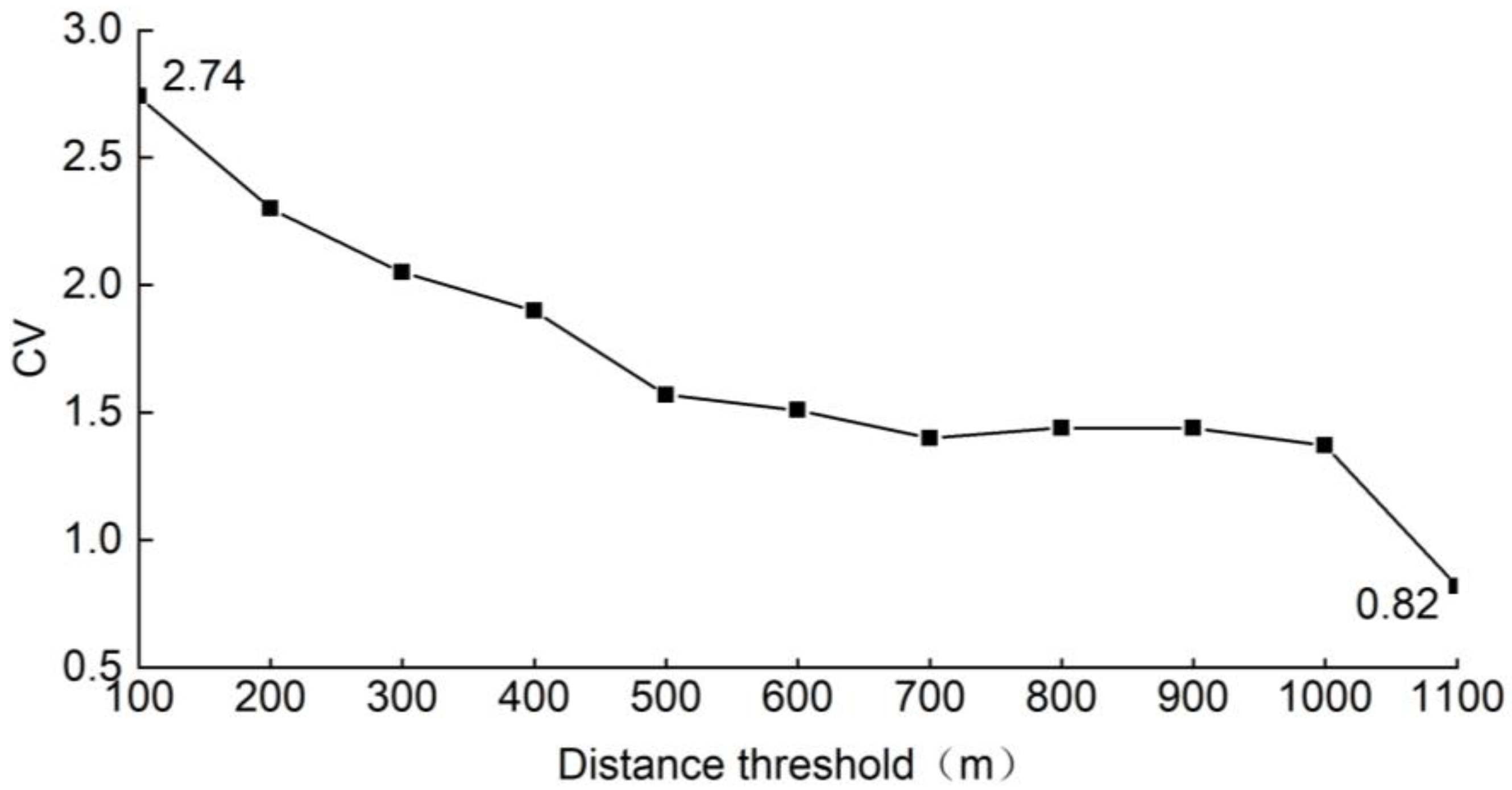
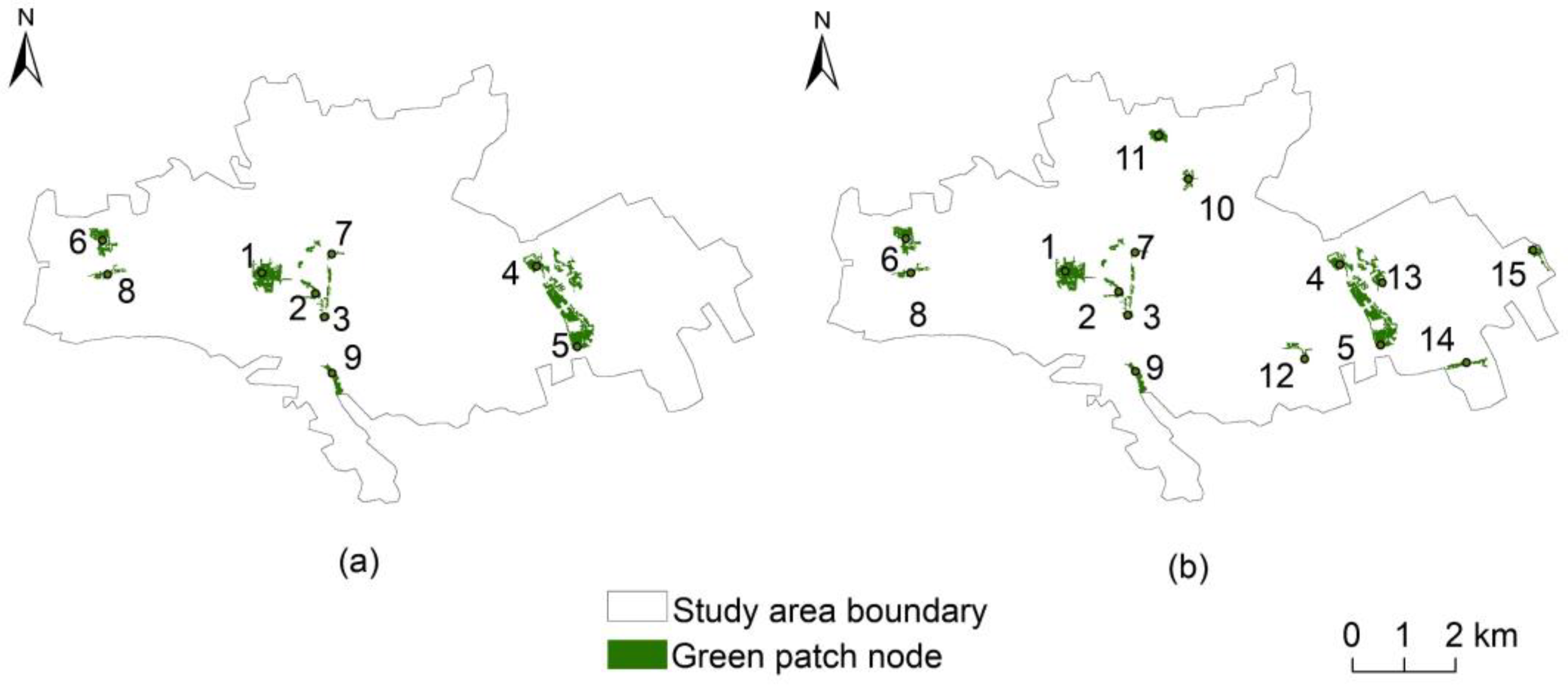
After identifying PC as a criterion for selecting nodes in a greenfield patch, we calculated its coefficient of variation. As shown in Figure 5, when the threshold value is 100 m, the coefficient of variation of the significant value of PC is the greatest (2.74), and the rank difference between patches in the research region is the greatest and most appropriate for selecting green space patch nodes. According to experience and high-definition images, the fragmentation of information about green patches in the research region is severe. There is a phenomenon of scattered tiny patches around large green patches, and it is vital to merge these tiny patches when matching park green patch information to more accurately depict a park’s green space. We selected the top 20 green spaces with a high dPC value beneath the 100 m threshold, matched or merged them with the green park space, and produced a total of 9 green spaces as nodes of the recreational green space network with a total area of 1.53 km² (Figure 6a).

Our green patch nodes selected by the connectivity index can match the popular parks in Kashgar City. The determined green patch nodes are mainly distributed in the study area’s east, middle, and west (Figure 6a). In the northern part of the study area, green space patches are usually small and spread out, with no critical green space patch nodes. The chosen green patch nodes have a high connectivity index and a high recreational value. East Lake Park, People’s Park, and Xiaoyalang Wetland Park are in the top five of the list of the hottest parks in the Kashgar region, as decided by the travel data on the different navigation maps (

Table 3. A list of the most popular parks in the Kashgar Region was obtained by searching on the navigation map (parks in Kashgar City) *.

	Navigation Map 1			Navigation Map 2
Park	Top	Number of People Who Have Navigated Recently/10,000 People	Reasons for Being on the List	Top	Number of People Who Have Navigated Recently/People	Reasons for Being on the List
East Lake Park	1	1.30	Night views, boating and walking	3	3279	Good for watching walks, relaxing
Xiao Yalang Wetland Park	3	1.50	Nice setting, easy access, good for walking	1	3694	Water landscape, suitable for leisure play
People’s park	5	1.30	The park is very big, the environment is very good, it is more suitable for daily leisure walks	2	2933	Beautiful scenery for a walk
West Park	8	0.84	Good for walking	6	1457	Exercise, walking
South Lake Park	15	0.28	Beautiful scenery for a walk	7	477	Good for walking
Dongcheng Park	-	-	-	11	174	Beautiful landscape

* The data comes from AutoNavi Map and Tencent Map, the list is updated to 4 October 2022.

). And Xiao Yalang Wetland Park has the highest number of recent visitors. The West Park is adjacent to Chalbagh Style Park; its popularity is second only to the three parks mentioned above. South Lake Park is close to East Park Park. Its popularity and number of visitors are not so many, but it still ranks at the top of the popular list in the entire Kashgar area. Dongcheng Park is next to Xiao Yalang Wetland Park and has good views, and is in the top 11 on one of the navigation maps. These parks are on the list because they provide beautiful scenery and are suitable for daily leisure walks or exercise. We find that the more popular the park, the more people come to enjoy the scenery and the recreation (Table 3), so we can use them as nodes in recreational networks.

According to the size of the area, we chose fifteen ecological green patches (Figure 6b), including almost most parkland with high recreational service value, with a total area of 3.18 square kilometers to cover the entire study area. We found that the new green space patch 10 belongs to protect green space, and patches 11–15 are five affiliated green spaces. In general, patches 1–15 are large green patches in the study area, containing more biological species, and can be used as the source of green patches for constructing a green space ecological network.

3.3. Potential Corridors

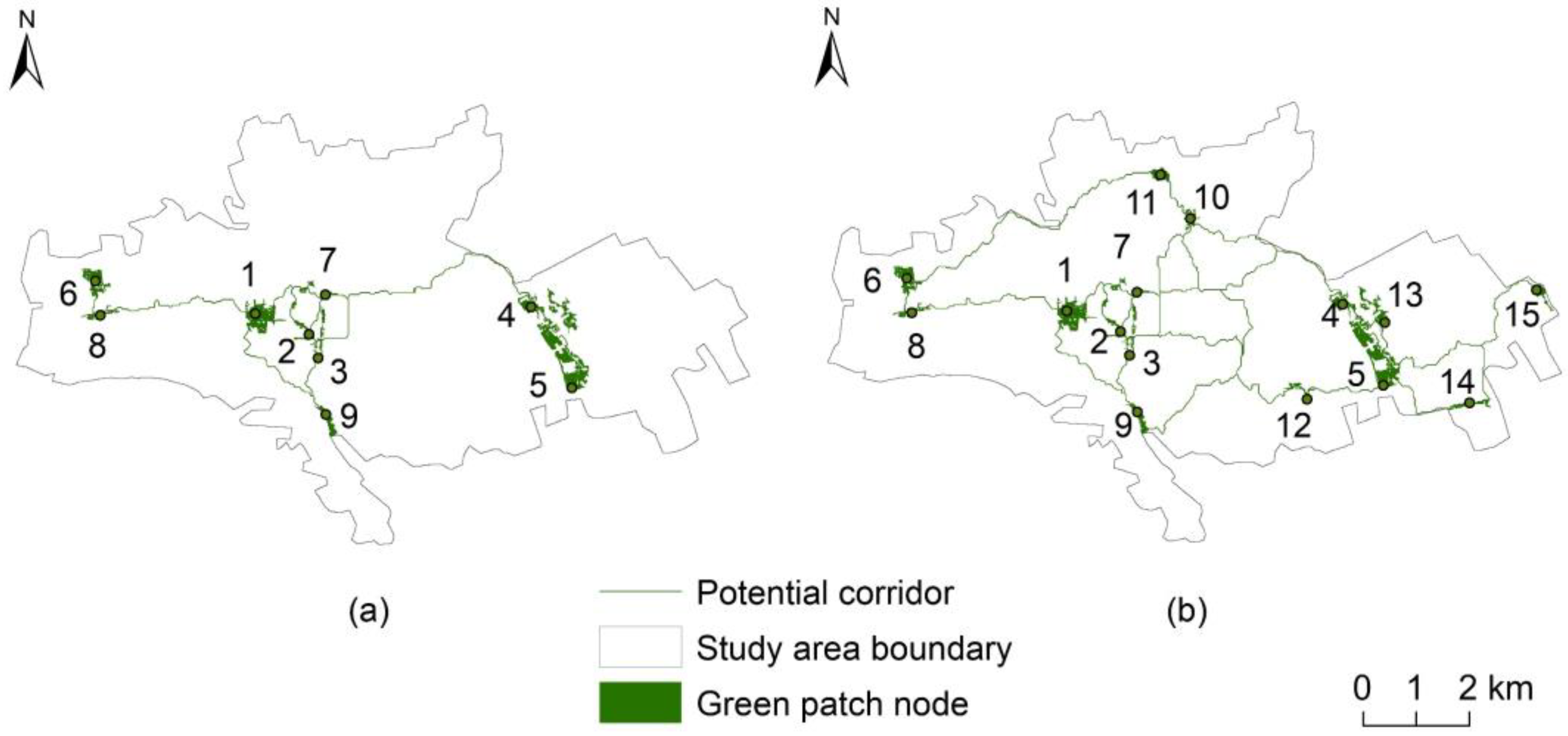
Our resistance values were assigned to various land cover types in the study region based on current research findings and actual conditions, and the cost surface is created. We used the least-cost path method to identify potential corridors. After removing redundant corridors between nodes, there were 24 potential recreational corridors between 29.25 m and 14.63 km long and 53 potential biodiversity conservation corridors between 18.87 m and 7.4 km long (Figure 7).

3.3.1. Distribution of Potential Green Space Corridors

Recreational corridors run from east to west in the study area, with a high density in the middle and a lower density to the east and west. There are no nodes of core green space patches or potential corridors in the north. The corridor linking patches 1, 8, and 6 connects People’s Park in the center to Charbagh style garden and West Park in the west. The corridor linking patches 2, 7, 4, and 5 connects East Lake Park to Xiao Yalang Wetland Park and Dongcheng Park in the east. The corridor linking patches 1, 7, 2, 3, and 9 connects People’s Park, East Lake Park, Times Square, South Lake Park, and the green space around the Kashgar River, forming the study area’s core green space corridors. The corridor linking patches 6, 8, 1, 7, 4, and 5 is the longest east-west corridor in the research area. The northern green space patches are tiny and don’t have more prominent, connected core green space patches. The corridors go through the urban area and connect the eastern and western parts of the study area. However, the corridor did not cover most of the northern part of the study area and the large area on both sides of East Lake Park. The distribution of recreational corridors in the study area is not comprehensive enough (Figure 7a).

The green patch nodes were chosen based on the size of the patch, and this simulation shows that there are 28 more potential biodiversity conservation corridors than recreational corridors (Figure 7b). Our ecological green space patches overlap with the recreational patches and contain larger areas of other types of green space. The new corridor linking patches 6, 10, 11, 4, 13, 5, and 15 was added to the north, centered on East Lake Park, to connect the large-area green space and additional green space in the north and east of the study area. The longest corridor linking patches 6–10 links West Park to patch 10. The corridor linking patches 1, 9, 12, 5, 14, and 15 have been added south of East Lake Park, with Patch 12 being a recreational boulevard belt.

3.3.2. Composition of Potential Corridors’ Land Classes

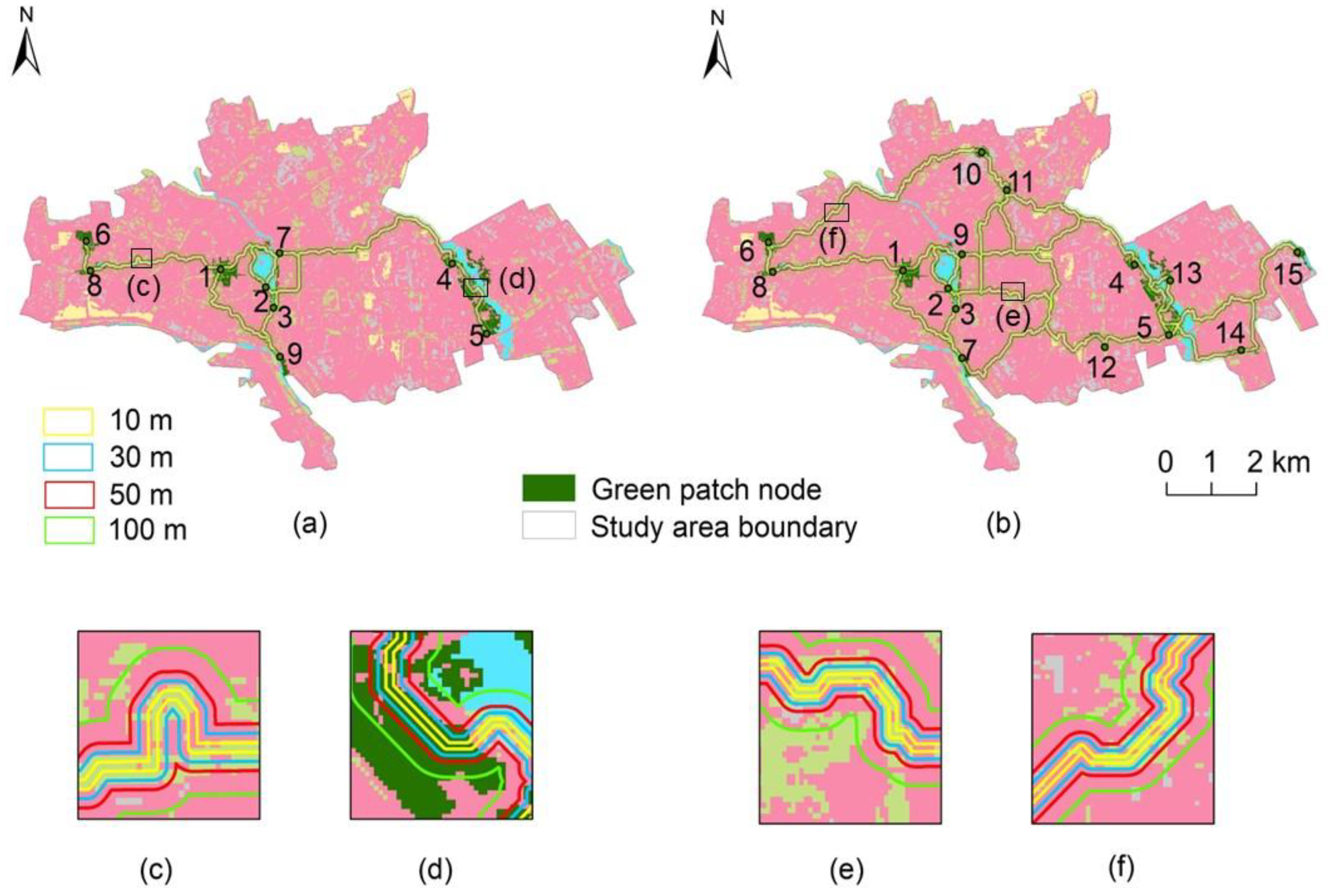
Our green space corridor level is urban land, where the land resources are scarce, which also needs to consider ecological benefits and space requirements for economic development. Therefore, it is particularly important to use the corridor buffer to determine the reasonable corridor width, to strengthen the rationale and science of the construction of green space networks. Under the premise of satisfying the migration and biological conservation functions of birds and small organisms [43], we selected the corridor buffer zone of 10 m, 30 m, 50 m, and 100 m for the width (Figure 8). We then determined appropriate corridor widths for the study area based on the proportion of different land use types within the buffer zone (

Table 4. Composition of the land class with different buffer zone distances for corridors with recreational potential.

Category	10 m		30 m		50 m		100 m
	S/ha	P/%	S/ha	P/%	S/ha	P/%	S/ha	P/%
Greenland	31.53	62.68	74.99	50.69	102.07	42.19	148.46	31.97
Construction	14.11	28.05	59.92	40.51	117.78	48.69	265.11	57.10
Agriculture	1.91	3.80	4.29	2.90	5.13	2.12	7.65	1.65
Water	2.18	4.33	7.24	4.89	13.94	5.76	34.95	7.53
Other	0.57	1.13	1.49	1.00	2.99	1.24	8.16	1.76
Sum	50.30	100.00	147.93	100.00	241.91	100.00	464.33	100.00

and

Table 5. Composition of the land class with different buffer zone distances for corridors with Ecotype potential.

Category	10 m		30 m		50 m		100 m
	S/ha	P/%	S/ha	P/%	S/ha	P/%	S/ha	P/%
Greenland	69.77	53.09	164.26	42.71	221.02	35.41	308.63	26.30
Construction	45.54	34.65	175.55	45.64	331.59	53.12	723.17	61.62
Agriculture	7.71	5.87	18.88	4.91	25.96	4.16	39.91	3.40
Waters	3.80	2.89	13.74	3.57	26.02	4.17	58.10	4.95
Other	4.59	3.47	12.19	3.17	19.63	3.14	43.71	3.72
Sum	131.41	100.00	384.62	100.00	624.22	100.00	1173.52	100.00

).

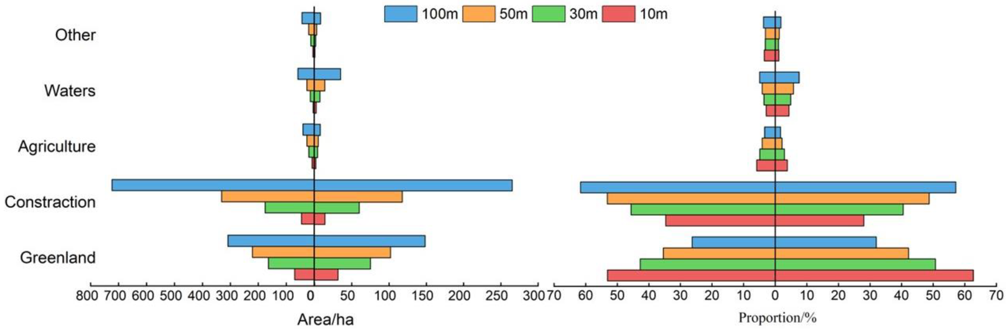
Among the five types of land cover in the study area, the degree of fluctuation of construction land area with the change of corridor buffer zone width is the largest. As the width of a corridor grows, the primary type of land use changes from urban green space to building land (Figure 9). Here, due to the complexity of land use types in built-up areas, we only consider the proportion of other landscape types, excluding construction land. When urban green space is the primary landscape type and the balance of construction land, the wider the corridor width, the better. In the 50 m corridor buffer zone, urban green space and construction land comprised more than 40 percent of the overall area. In contrast, agricultural land, water, and other land types were less than 6 percent. After the width of the corridor buffer zone surpasses 50 m, the land use type ratio in the corridor is dominated by building land, which is not conducive to species migration and energy diffusion across patches (Table 4). Within the 30 m buffer zone of biodiversity conservation corridors, urban green land and building land both account for more than 40% of the land types occupied by potential corridors. Comparatively, agricultural land, water, and other land types make up less than 5 %. After the buffer distance exceeds 30 m, the proportion of construction land exceeds that of urban green space and other lands, which is also detrimental to the corridor’s function. In conclusion, urban green space is the primary type of landscape of the potential corridor within the 50 m buffer zone of the recreational corridor and the 30 m buffer zone of the ecological corridor in the built-up area, which means that the corridor width is more appropriate.

3.4. Corridor Curvature

3.4.1. Construction of an Integrated Network of Green Spaces

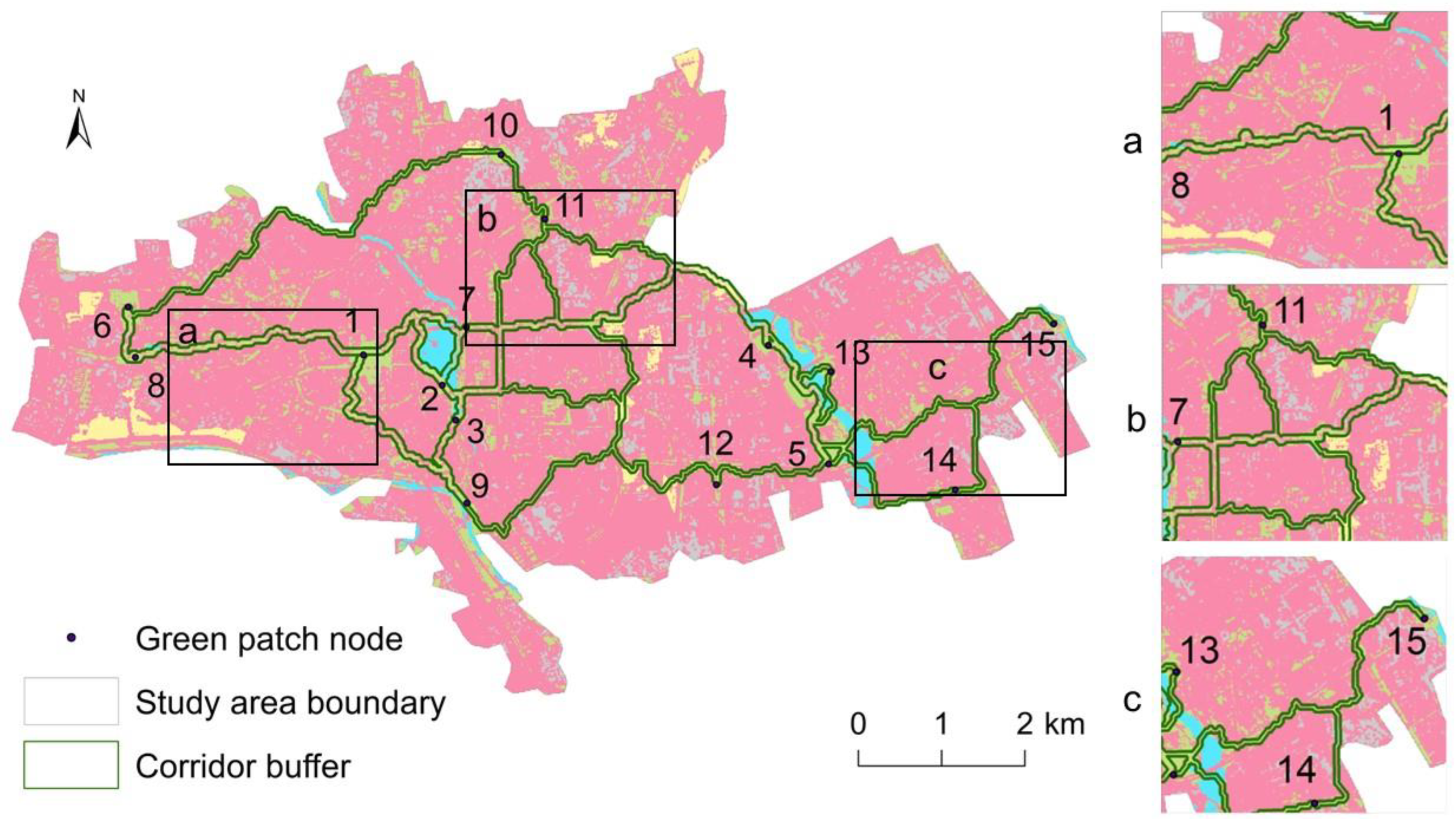
Our 30 m buffer zone of the potential ecological corridor was combined with the 50 m buffer zone of the recreation type to create a comprehensive network of green space with recreational service and ecological and environmental value (Figure 10). Ecological green space patches include all green space patches that source recreational corridors. Our network of integrated green spaces can meet the movement of birds and small mammals and includes recreational corridors with parks as the main nodes.

3.4.2. Corridor Curvature

Table 6. Corridors matrix based on the corridor curvature.

Patch	1	2	3	4	5	6	7	8	9	10	11	12	13	14	15
1	0	1.99	1.78	1.78	1.46	1.44	1.25	1.23	1.18	1.47	1.26	1.51	1.37	1.58	1.67
2		0	1.39	1.43	1.49	1.59	1.00	1.46	1.25	1.37	1.14	1.51	1.70	1.43	1.68
3			0	1.60	1.59	1.62	1.25	1.52	1.24	1.37	1.25	1.69	1.86	1.65	1.65
4				0	1.32	1.37	1.30	1.29	1.65	1.17	1.13	1.79	1.82	1.73	1.96
5					0	1.47	1.47	1.53	1.50	1.39	1.39	1.28	1.25	1.40	1.45
6						0	1.41	1.28	1.50	1.31	1.49	1.55	1.40	1.47	1.57
7							0	1.25	1.25	1.65	1.37	1.64	1.38	1.57	1.73
8								0	1.42	1.42	1.62	1.47	1.32	1.42	1.53
9									0	1.32	1.22	1.61	1.71	1.45	1.49
10										0	1.38	1.51	1.36	1.38	1.66
11											0	1.57	1.41	1.33	1.66
12												0	1.61	1.36	1.42
13													0	1.65	2.15
14														0	1.37
15															0

demonstrates that curvature values between patches 2 and 7, between 2 and 11, and between 4 and 11 are small, with values of 1.00, 1.14, and 1.15. Because these three corridors aren’t as curved, it’s easier for organisms and energy to move and spread from one patch to another. So, when planning green space, we can add patches of green space between patches 7 and 11 and patches 4 and 11 to give more green open spaces and biological habitats. With a value of 2.15, 1.99, and 1.96, patches 13 and 15, between 1 and 2, and between 4 and 15 have the most curved corridors, meaning the corridors are more complicated than those in other patches, and the rate of biological movement will become lower. Because there aren’t any continuous green patches between patch 13 (Xiao Yalang Wetland Park) and patch 15 (green spaces around the Shang Yalang Reservoir), the corridor between them has to go around construction sites and other high-resistance areas. Similarly, the green space patches between patches 1 and 2 and patches 4 and 15 are sparse, fragmented, and discontinuous. So, planning for green belts should “identify gaps and inject green”, making it much easier to build green infrastructure between buildings and on both sides of roads. As the living environment is improved, we will add more bird and animal habitats to promote connections, and reduce fragmentation.

4. Discussion

4.1. Effects of Selecting Green Patches on Corridors by Different Methods

Compared with previous studies, this paper uses two methods when selecting green patches [24,35,47]. We identified the patches (nodes) based on the area size and connection index of green space patches. We find we can match the geographic position of the chosen patches based on the connection index to the location of the green park space in the study area with a high recreational service value. That is not seen in previous articles using the same method [24,34]. And the potential recreational corridors are distributed in an east-west direction, clustering most densely in Central People’s Park and East Lake Park, highlighting the social and economic benefits. However, the green patches selected based on the patch area size have more green types and biodiversity [35]. The generated potential corridors connect the large green patches in the study area, and the constructed green space network covers the research area, highlighting the biodiversity protection function of the corridor [36].

To some extent, determining the appropriate corridor width could serve as a guideline for enhancing the green space network’s structural integrity and sustaining the city’s biodiversity. However, few studies consider green spaces’ health, recreation, and biodiversity conservation functions to construct urban green space networks while considering reasonable corridor widths according to the different functions. Based on the identification of the above two corridor networks, we consider their widths separately. We mainly considered the effect of land use type on corridor width [55]. Following analysis, in built-up urban areas, when the dominant landscape type is urban green space and balanced with construction land, the continuity of the corridor is ensured to the greatest extent. We determined that the width of the recreational green space network corridor generated by selecting patches based on connectivity is 50 m, connecting popular parks in the built-up area. That enhances connectivity between parks, provides a green open space for people who enjoy walking and running, and promotes physical and mental health [9,55]. The width of the ecological green space network corridor generated by selecting patches based on area size is 30 m, which allows for bird migration (10 meters or more) and safeguards invertebrates like ants, earthworms, and grasshoppers (9–12 m) [43,56]. Due to the complexity of land use in urban built-up areas, other studies have argued that the factors affecting the corridor width still need further exploration [55].

In summary, selecting green patches by different methods will impact corridors’ function, distribution, and width. The comprehensive green space network constructed in this paper can protect the city’s biodiversity. It connects to popular parks and can also be a suitable place for people to walk, run or do other recreational activities with health functions.

4.2. Advantages and Disadvantages of Land Type Assignment and Construction of Cost Surface

Many green space network construction studies use the expert scoring method for creating cost surfaces. The advantages of this approach include its simplicity, reduced data requirements, and ability to describe significant variations in energy and organism movement rates and diffusion between different terrain types [14,57]. According to the research that has been conducted thus far, the relative amounts of resistance to each type of urban land are as follows: construction land > other lands > water > agricultural land > green spaces. Still, there is no standard for expressing any land cover’s absolute magnitude of resistance. The resistance values for different land-use types, according to Wu Zhen et al., are 10 for green space, 600 for water, 50 for agricultural land, 1000 for construction land, and 700 for other lands; other studies [58] used 1–5 to illustrate the increasing ecological resistance values for different land-use types. Urban landscapes are highly fragmented, urban land use patterns are diverse, and urban ecological processes are complex. It is difficult to assign homogenized values to land uses that accurately reflect resistance differences within the same land-use type [59]. We excluded common criteria such as elevation, slope, and distance from the cost surface screening after studying the actual conditions of the study region. Our cost surface was then created using the conventional homogenization assignment of land use.

4.3. Prospects and Suggestions for Green Space Network Planning in the Study Area

In this paper, similar with other research studies such as by Kong et al. [14], and Wu Zhen et al. [24], We can determine the distribution of green space, identify high-quality green space patches and corridors, and identify corridors or patches that can be protected or developed. At the same time, we explore corridor widths in urban built-up areas, rarely covered by previous studies. The width of the corridor is not the wider the better [55]. Because in the built-up area of the city, as the width of the corridor increases, the construction land occupies more and more space. Our width range of recreational corridors is larger than that of biodiversity conservation corridors. That is because the distribution of green space in Kashgar is uneven, the distribution of green space services is uneven, and the construction of green corridors is not in place. Therefore, in green space planning, we should pay attention to the functionality and uniformity of the distribution of large green space patches while reducing fragmentation and enhancing connectivity. By building park systems and putting up greenbelts, cities make the most of their green space eco-space [60]. To highlight the “people-oriented” concept of green space planning and emphasize the inclusive distribution of parks. We may solve the uneven distribution of green spaces by constructing new green areas at the source of the green space network. Also, we should coordinate urban greening by making green urban highways and urban shelter forests.

The strategy of ecological civilization and the concept of green development requires the full use of the multiple functions of urban green space to promote the city’s beautiful, livable, and sustainable development. In light of this, raising the level of urban green space planning and enhancing its scientific component has become an essential objective in the preparation and management of urban green space planning. We found the issues of inadequate green space planning, uneven green space distribution, and fragmentation in Kashgar City by developing a comprehensive potential green space network in urban districts. Relevant research results can help reduce the fragmentation of urban ecological landscapes, stabilize the urban ecological structure, and encourage urban green spaces to have more social, economic, and ecological benefits.

5. Conclusions

We first take Kashgar City Center, a city in arid regions, as the study area to explore constructing a small-scale green space network. The study identifies corridors for recreational services and biodiversity conservation. It determines reasonable corridor widths based on the proportion of land use types with different corridor buffer widths, which has rarely been discussed in previous literature. Among the study’s primary findings are:

(1)

In Kashgar, the degree of landscape fragmentation is relatively high. There are enormous green patches in the north of the study zone, but there is poor connectivity; the eastern green corridor has a complicated curvature and lacks small green patches interacting with one another.

(2)

The urban green space network of Kashgar City, which is constructed by green patches selected based on connectivity and area size, dominates recreation and biodi-versity conservation functions. We can find that the recreational corridors linking the park completely overlap with the biodiversity conservation corridors linking large areas of green space.

(3)

The most appropriate widths of recreational and biodiversity conservation corridor buffers were derived by analyzing the composition of characteristics within the corridor buffer zone. We constructed a comprehensive green space network. It can provide green open space for residents to walk or run daily and a resting place for some biological species in the city.

(4)

The urban green space planning of Kashgar City can refer to our suggestion to protect important green spaces or increase green patches based on the simulated green space network. That will help to improve and optimize the urban green space structure, protect the urban ecological environment and biodiversity, meet the varied demands of various biological components on the green space system in the city, and better reflect the service value of urban green space.

References

- Gascon, M.; Triguero-Mas, M.; Martinez, D.; Dadvand, P.; Forns, J.; Plasencia, A.; Nieuwenhuijsen, M.J. Mental health benefits of long-term exposure to residential green and blue spaces: A systematic review. Int. J. Env. Res. Public Health 2015, 12, 4354–4379. [Google Scholar] [CrossRef] [PubMed] [Green Version]
- Twohig-Bennett, C.; Jones, A. The health benefits of the great outdoors: A systematic review and meta-analysis of greenspace exposure and health outcomes. Environ. Res. 2018, 166, 628–637. [Google Scholar] [CrossRef] [PubMed]
- Holt, E.W.; Lombard, Q.K.; Best, N.; Smiley-Smith, S.; Quinn, J.E. Active and Passive Use of Green Space, Health, and Well-Being amongst University Students. Int. J. Environ. Res. Public Health 2019, 16, 424. [Google Scholar] [CrossRef] [PubMed] [Green Version]
- Reyes-Riveros, R.; Altamirano, A.; De la Barrera, F.; Rozas-Vasquez, D.; Vieli, L.; Meli, P. Linking public urban green spaces and human well-being: A systematic review. Urban For. Urban Green. 2021, 61, 127105. [Google Scholar] [CrossRef]
- Lee, A.C.K.; Maheswaran, R. The health benefits of urban green spaces: A review of the evidence. J. Public Health 2010, 33, 212–222. [Google Scholar] [CrossRef] [Green Version]
- Markevych, I.; Schoierer, J.; Hartig, T.; Chudnovsky, A.; Hystad, P.; Dzhambov, A.M.; De Vries, S.; Triguero-Mas, M.; Brauer, M.; Nieuwenhuijsen, M.J. Exploring pathways linking greenspace to health: Theoretical and methodological guidance. Environ. Res. 2017, 158, 301–317. [Google Scholar] [CrossRef]
- Cusack, L.; Larkin, A.; Carozza, S.; Hystad, P. Associations between residential greenness and birth outcomes across Texas. Environ Res 2017, 152, 88–95. [Google Scholar] [CrossRef]
- Gubbels, J.S.; Kremers, S.P.; Droomers, M.; Hoefnagels, C.; Stronks, K.; Hosman, C.; de Vries, S. The impact of greenery on physical activity and mental health of adolescent and adult residents of deprived neighborhoods: A longitudinal study. Health Place 2016, 40, 153–160. [Google Scholar] [CrossRef]
- Venter, Z.S.; Barton, D.N.; Gundersen, V.; Figari, H.; Nowell, M. Urban nature in a time of crisis: Recreational use of green space increases during the COVID-19 outbreak in Oslo, Norway. Environ. Res. Lett. 2020, 15, 104075. [Google Scholar] [CrossRef]
- Guillen-Cruz, G.; Rodríguez-Sánchez, A.L.; Fernández-Luqueño, F.; Flores-Rentería, D. Influence of vegetation type on the ecosystem services provided by urban green areas in an arid zone of northern Mexico. Urban For. Urban Green. 2021, 62, 127135. [Google Scholar] [CrossRef]
- Selmi, W.; Weber, C.; Rivière, E.; Blond, N.; Mehdi, L.; Nowak, D. Air pollution removal by trees in public green spaces in Strasbourg city, France. Urban For. Urban Green. 2016, 17, 192–201. [Google Scholar] [CrossRef] [Green Version]
- Lepczyk, C.A.; Aronson, M.F.J.; Evans, K.L.; Goddard, M.A.; Lerman, S.B.; MacIvor, J.S. Biodiversity in the City: Fundamental Questions for Understanding the Ecology of Urban Green Spaces for Biodiversity Conservation. BioScience 2017, 67, 799–807. [Google Scholar] [CrossRef] [Green Version]
- Opdam, P. Metapopulation theory and habitat fragmentation: A review of holarctic breeding bird studies. Landsc. Ecol. 1991, 5, 93–106. [Google Scholar] [CrossRef]
- Kong, F.; Yin, H.; Nakagoshi, N.; Zong, Y. Urban green space network development for biodiversity conservation: Identification based on graph theory and gravity modeling. Landsc. Urban Plan. 2010, 95, 16–27. [Google Scholar] [CrossRef]
- Saboonchi, P.; Abarghouyi, H.; Motedayen, H. Green Landscape Networks;The role of articulation in the integrity of green space in landscapes of contemporary cities of Iran. Bagh-E Nazar 2018, 15, 5–16. [Google Scholar] [CrossRef]
- Jongman, R. Ecological networks are an issue for all of us. J. Landsc. Ecol. 2008, 1, 7–13. [Google Scholar] [CrossRef] [Green Version]
- Song, S.; Wang, S.-H.; Shi, M.-X.; Hu, S.-S.; Xu, D.-W. Multiple scenario simulation and optimization of an urban green infrastructure network based on complex network theory: A case study in Harbin City, China. Ecol. Process. 2022, 11, 1–16. [Google Scholar] [CrossRef]
- Little, C.E. Greenways for America; Johns Hopkins University Press: Baktimore, MD, USA; London, UK, 1990. [Google Scholar]
- Tzoulas, K.; James, P. Peoples’ use of, and concerns about, green space networks: A case study of Birchwood, Warrington New Town, UK. Urban For. Urban Green. 2010, 9, 121–128. [Google Scholar] [CrossRef] [Green Version]
- Jim, C.Y.; Chen, S.S. Comprehensive greenspace planning based on landscape ecology principles in compact Nanjing city, China. Landsc. Urban Plan. 2003, 65, 95–116. [Google Scholar] [CrossRef]
- Li, F.; Wang, R.; Paulussen, J.; Liu, X. Comprehensive concept planning of urban greening based on ecological principles: A case study in Beijing, China. Landsc. Urban Plan. 2005, 72, 325–336. [Google Scholar] [CrossRef]
- Uy, P.D.; Nakagoshi, N. Application of land suitability analysis and landscape ecology to urban greenspace planning in Hanoi, Vietnam. Urban For. Urban Green. 2008, 7, 25–40. [Google Scholar] [CrossRef]
- Zhang, L.; Peng, J.; Liu, Y.; Wu, J. Coupling ecosystem services supply and human ecological demand to identify landscape ecological security pattern: A case study in Beijing–Tianjin–Hebei region, China. Urban Ecosyst. 2017, 20, 701–714. [Google Scholar] [CrossRef]
- Wu, Z.; Wang, H. Establishment and optimization of green ecological networks in Yangzhou City. Chin. J. Ecol. 2015, 34, 1976–1985. [Google Scholar]
- Cui, L.; Wang, J.; Sun, L.; Lv, C. Construction and optimization of green space ecological networks in urban fringe areas: A case study with the urban fringe area of Tongzhou district in Beijing. J. Clean. Prod. 2020, 276, 124266. [Google Scholar] [CrossRef]
- Mougiakou, E.; Photis, Y.N. Urban green space network evaluation and planning: Optimizing accessibility based on connectivity and raster gis analysis. Eur. J. Geogr. 2014, 5, 19–46. [Google Scholar]
- Jian, S.; Zhang, Q.; Tao, H. Construction and evaluation of green space ecological network in Guangzhou. Acta Sci. Nat. Univ. Sunyatseni 2016, 55, 162–170. [Google Scholar]
- Wang, J.; Rienow, A.; David, M.; Albert, C. Green infrastructure connectivity analysis across spatiotemporal scales: A transferable approach in the Ruhr Metropolitan Area, Germany. Sci. Total Environ. 2022, 813, 152463. [Google Scholar] [CrossRef]
- Saura, S.; Vogt, P.; Velázquez, J.; Hernando, A.; Tejera, R. Key structural forest connectors can be identified by combining landscape spatial pattern and network analyses. For. Ecol. Manag. 2011, 262, 150–160. [Google Scholar] [CrossRef]
- Wickham, J.D.; Riitters, K.H.; Wade, T.G.; Vogt, P. A national assessment of green infrastructure and change for the conterminous United States using morphological image processing. Landsc. Urban Plan. 2010, 94, 186–195. [Google Scholar] [CrossRef]
- Vogt, P.; Riitters, K.H.; Iwanowski, M.; Estreguil, C.; Kozak, J.; Soille, P.J.E.i. Mapping landscape corridors. Ecol. Indic. 2007, 7, 481–488. [Google Scholar] [CrossRef]
- Huang, H.; Yu, K.; Gao, Y.; Liu, J. Building Green Infrastructure Network of Fuzhou Using MSPA. Chin. Landsc. Archit. 2019, 35, 70–75. [Google Scholar]
- Guo, W.; Yu, L.; Sun, Y.; Chen, P. Ecological network planning of urban green space in urban center of Shunde District, Foshan City, Guangdong Province of South China. Chin. J. Ecol. 2012, 31, 1022–1027. [Google Scholar]
- Li, S.; Li, T.; Peng, Z.; Huang, Z.; Qi, Z. Construction of green space ecological network in Dongting Lake region with comprehensive evaluation method. Chin. J. Appl. Ecol. 2020, 31, 2687–2698. [Google Scholar]
- Kong, F.; Yin, H. Developing green space ecological networks in Jinan City. Acta Ecol. Sin. 2008, 4, 1711–1719. [Google Scholar]
- Teng, M.; Wu, C.; Zhou, Z.; Elizabeth, L.; Zheng, Z. Multipurpose greenway planning for changing cities: A framework integrating priorities and a least-cost path model. Landsc. Urban Plan. 2011, 103, 1–14. [Google Scholar] [CrossRef]
- Yuan, Z.; Zhao, M.; Liu, R. Construction and optimization of urban green space network based on minimun cost distance and improved gravity model. J. Shaanxi Norm. Univ. 2017, 45, 104–109. [Google Scholar]
- Gao, Y.; Mu, H.; Zhang, Y.; Tian, Y.; Tang, D.; Li, X. Research on construction path optimization of urban-scale green network systembased on MSPA analysis method: Taking Zhaoyuan City as an example. Acta Ecol. Sin. 2019, 39, 7547–7556. [Google Scholar]
- Hao, L.; Xiao, Z.; Deng, R.; Wanf, W. The Construction of Greenway Ecological Network Coupling with Urban Space in the Central Urban Area of Zhengzhou. Ecol. Econ. 2019, 35, 224–229. [Google Scholar]
- Kaur, R.; Gupta, K. Blue-Green Infrastructure (BGI) network in urban areas for sustainable storm water management: A geospatial approach. City Environ. Interact. 2022, 16, 100087. [Google Scholar] [CrossRef]
- Li, S.; Xiao, W.; Zhao, Y.; Lv, X. Incorporating ecological risk index in the multi-process MCRE model to optimize the ecological security pattern in a semi-arid area with intensive coal mining: A case study in northern China. J. Clean. Prod. 2020, 247, 119143. [Google Scholar] [CrossRef]
- Donati, G.F.A.; Bolliger, J.; Psomas, A.; Maurer, M.; Bach, P.M. Reconciling cities with nature: Identifying local Blue-Green Infrastructure interventions for regional biodiversity enhancement. J. Environ. Manag. 2022, 316, 115254. [Google Scholar] [CrossRef] [PubMed]
- Zhu, Q.; Yu, K.; Li, D. The width of ecological corridor in landscape planning. Acta Ecol. Sin. 2005, 25, 2406–2412. [Google Scholar]
- Semeraro, T.; Scarano, A.; Buccolieri, R.; Santino, A.; Aarrevaara, E. Planning of Urban Green Spaces: An Ecological Perspective on Human Benefits. Land 2021, 10, 105. [Google Scholar] [CrossRef]
- Li, X.; Fang, C.; Huang, J.; Mao, H. The Urban Land Use Transformations and Associated Effects on Eco-Environment in Northwest China Arid Region: A Case Study in Hexi Region, Gansu Province. Quat. Sci. 2003, 23, 280–290+348–349. [Google Scholar]
- Liu, J.; Kuang, W.; Zhang, Z.; Xu, X.; Qin, Y.; Ning, J.; Zhou, W.; Zhang, S.; Li, R.; Yan, C.; et al. Spatiotemporal characteristics, patterns and causes of land usechanges in China since the late 1980s. Acta Geogr. Sin. 2014, 24, 195–210. [Google Scholar]
- Shi, H.; Xu, Y. Research on planning method of urban green space core region based on landscape connectivity. J. Nanjing For. Univ. 2011, 35, 51–56. [Google Scholar]
- Saura, S.; Torné, J. Conefor Sensinode 2.2: A software package for quantifying the importance of habitat patches for landscape connectivity. Environ. Model. Softw. 2009, 24, 135–139. [Google Scholar] [CrossRef]
- Saura, S.; Pascual-Hortal, L. A new habitat availability index to integrate connectivity in landscape conservation planning: Comparison with existing indices and application to a case study. Landsc. Urban Plan. 2007, 83, 91–103. [Google Scholar] [CrossRef]
- Shi, H.; Xian, M.; Xu, Y.; Xue, J.; Liu, H. Developing Integrated Methods to Construct Urban Potential Green Corridors:A Case Study of Changzhou City. Sci. Silvae Sin. 2013, 49, 92–100. [Google Scholar]
- Xu, J. Mathematical Methods in Modern Geography; Higher Education Press: Beijing, China, 2002. [Google Scholar]
- Adriaensen, F.; Chardon, J.P.; De Blust, G.; Swinnen, E.; Villalba, S.; Gulinck, H.; Matthysen, E. The application of ‘least-cost’ modelling as a functional landscape model. Landsc. Urban Plan. 2003, 64, 233–247. [Google Scholar] [CrossRef]
- Goodwin, B.J.; Fahrig, L. Effect of landscape structure on the movement behaviour of a specialized goldenrod beetle, Trirhabda borealis. Can. J. Zool. 2002, 80, 24–35. [Google Scholar] [CrossRef] [Green Version]
- Wang, J.; Wang, H. An Analysis of the New Standard for Classification of Urban Green Space. Chin. Landsc. Archit. 2019, 35, 92–95. [Google Scholar]
- Peng, J.; Zhao, H.; Liu, Y. Urban ecological corridors construction: A review. Acta Ecol. Sin. 2017, 37, 23–30. [Google Scholar] [CrossRef]
- Newbold, J.D.; Erman, D.C.; Roby, K.B. Effects of Logging on Macroinvertebrates in Streams With and Without Buffer Strips. Can. J. Fish. Aquat. Sci. 1980, 37, 1076–1085. [Google Scholar] [CrossRef]
- Yang, K.; Cao, Y.; Feng, Z.; Geng, B.; Feng, Y.; Wang, S. Research Progress of Ecological Security Pattern Construction Based on Minimum Cumulative Resistance Model. J. Ecol. Rural Environ. 2021, 37, 555–565. [Google Scholar]
- Wang, M.; Liang, S. Health City Oriented Green Space Ecological Network Planning in Central Urban Area of Taiyuan. Planners 2021, 37, 44–50, 56. [Google Scholar]
- Hepcan, Ç.C.; Özkan, M.B. Establishing ecological networks for habitat conservation in the case of Çeşme–Urla Peninsula, Turkey. Environ. Monit. Assess. 2011, 174, 157–170. [Google Scholar] [CrossRef]
- Liu, H.; Yang, M.; Li, B.; Guo, S.; Gu, X. Urban Green Corridor System Planning Based on Ecological Security—Taking Nanchang City as the Example. Chin. Landsc. Archit. 2020, 36, 122–127. [Google Scholar]
Figure 1.
Study area.
Figure 2.
The process used to identify potential corridors and develop an urban green space network.
Figure 3.
Spatial distribution of urban land use in Kashgar city.
Figure 4.
Spearman rank correlations between the values under different distance thresholds.
Figure 5.
Coefficient of variation of values under different distance thresholds.
Figure 6.
Spatial distribution of the selected green patch nodes: (a) recreational green space nodes; (b) ecological green space patch nodes. Note: (1) People’s Park; (2) East Lake Park; (3) South Lake Park; (4) Xiao Yalang Wetland Park; (5) Dongcheng Park; (6) West Park; (7) Times Squar; (8) Chalbagh Style Park; (9) Kashgar River; (10) Woodland; (11) Xiangfei Garden; (12) Shade belt; (13) Woodland; (14) Kashgar University; (15) Shang Yalang Reservoir.
Figure 7.
Potential urban green space network based on the least-cost path method: (a) recreational corridors; (b) ecological corridors. Note: (1) People’s Park; (2) East Lake Park; (3) South Lake Park; (4) Xiao Yalang Wetland Park; (5) Dongcheng Park; (6) West Park; (7) Times Squar; (8) Chalbagh Style Park; (9) Kashgar River; (10) Woodland; (11) Xiangfei Garden; (12) Shade belt; (13) Woodland; (14) Kashgar University; (15) Shang Yalang Reservoir.
Figure 8.
Potential green space networks based on buffers of different distances: (a) recreational network; (b) biodiversity conservation network. Note: (1) People’s Park; (2) East Lake Park; (3) South Lake Park; (4) Xiao Yalang Wetland Park; (5) Dongcheng Park; (6) West Park; (7) Times Squar; (8) Chalbagh Style Park; (9) Kashgar River; (10) Woodland; (11) Xiangfei Garden; (12) Shade belt; (13) Woodland; (14) Kashgar University; (15) Shang Yalang Reservoir; (c–f) are detail images.
Figure 9.
Changes in land use in buffer zones at different distance from potential corridors.
Figure 10.
Construction of an urban green space network. Note: (1) People’s Park; (2) East Lake Park; (3) South Lake Park; (4) Xiao Yalang Wetland Park; (5) Dongcheng Park; (6) West Park; (7) Times Squar; (8) Chalbagh Style Park; (9) Kashgar River; (10) Woodland; (11) Xiangfei Garden; (12) Shade belt; (13) Woodland; (14) Kashgar University; (15) Shang Yalang Reservoir; (a–c) are detail images.