Assessment of Land-Use Scenarios at a National Scale Using Intensity Analysis and Figure of Merit Components

Abstract

To address the impacts of future land changes on biodiversity and ecosystem services, land-use scenarios have been developed at the national scale in Japan. However, the validation of land-use scenarios remains a challenge owing to the lack of an appropriate validation method. This research developed land-use maps for 10 land-use categories to calibrate a land-change model for the 1987–1998 period, simulate changes during the 1998–2014 period, and validate the simulation for the 1998–2014 period. Following an established method, this study assessed the three types of land change: (1) reference change during the calibration time interval, (2) simulation change during the validation time interval, and (3) reference change during the validation time interval, using intensity analysis and figure of merit components (hits, misses, and false alarms). The results revealed the cause of the low accuracy of the national scale land-use scenarios as well as priority solutions, such as aligning the underlying spatial vegetation maps and improving the model to reduce two types of disagreement between the simulation and reference maps. These findings should help to improve the accuracy of model predictions and help to better inform policymakers during the decision-making process.

1. Introduction

Land-use models have been used to project future changes with the aim of supporting decision-making by policymakers [1]. The Intergovernmental Science-Policy Platform on Biodiversity and Ecosystem Services encouraged the use of modeling approaches to predict ecosystem changes based on possible future scenarios [2] because the use of scenarios allows information to be synthesized and streamlines key messages to facilitate communication with policymakers [3]. In Japan, national-scale future scenarios (the Predicting and Assessing Natural Capital and Ecosystem Services (PANCES) scenarios) were developed based on surveys and expert discussions with the aim of assessing the quantity of future changes in ecosystem services through 2050 [4]. Population and land-use modeling have been further conducted to translate these qualitative scenario storylines into quantitative simulations [5,6,7].

As the conventional classifications of land use and land cover (LULC) categories are too limited to sufficiently assess ecosystem services, especially in Asia where different vegetation types exist, national-scale land-use scenarios using newer datasets derived from vegetation inventory data were developed with nine LULC categories at the special resolution of 1 km² to enable sufficient assessment of natural capital and ecosystem services [7]. The PANCES land-use scenarios revealed the consequences of land-use interventions in a plausible future in Japan, including land abandonment and the underutilization of natural resources, which are currently a critical concern because of depopulation and an aging society. However, the requirement of fine spatial resolution is still a challenge in modeling agricultural land abandonment, which has been expanding in many areas throughout the country in the past few decades. Generally, a resolution of 1 km² is too coarse to detect these land transitions, and finer spatial resolution and updated data are required to detect the critical land transitions related to farmland abandonment [8].

Verifying and validating models as well as assessing and managing uncertainty in scenario analysis are also often critical, as, otherwise, the analysis can rest on unsupported assumptions and limited data [9]. The PANCES land-use scenarios were developed using Land Change Modeler, a land change model tool that empirically models relationships of explanatory variables of observed land changes and simulates future scenarios [10]. These land-use scenarios showed key land changes as consequences of intensive/extensive land-use interventions and regional differences in the gains and losses of each LULC category in each scenario. However, the accuracy assessment measure, figure of merit (FOM; defined in Section 2.4), was low for the simulation results, and this remains an important issue in terms of the credibility of the quantitative scenarios showing policy impacts [7]. In processing the PANCES land-use scenarios, past LULC maps (1987 and 1998) were used in the change analyses to detect historical patterns of land change. Existing and dominant transitions were identified in these analyses to be modeled in the prediction processes. Predictions were made using transition matrices adjusted to produce future land-use demands that would meet government land-use policies and the narratives of the PANCES scenarios. The transition modeling might, however, be limited in its description of the transitions relating to land abandonment, which, along with depopulation, began to increase around 2010. As such, an updated dataset would need to detect current land change trends.

To improve the land-use predictions, we need to know what is missing from the existing model and what needs to be improved. Validation using a single metric has been used to assess the multiple outputs and select the best model—that is, the one with the best fit to the observations. However, validation from a collection of metrics might generate insights that are deeper than any single metric can communicate [11]. Varga et al. [11] recommended a visual and quantitative comparison of changes during two time intervals: the reference change during the calibration interval and simulation change and the reference change during the validation interval. In this way, we can observe calibration patterns in subsequent simulations as well as distinguish between simulation and reference changes during the validation interval and the degree to which the reference patterns are stationary through time. Intensity analysis can reveal various levels of information concerning quantity disagreement, and FOM components (hits, misses, and false alarms) can distinguish quantity disagreement from allocation disagreement during the validation interval. Distinguishing quantity disagreement from allocation disagreement is particularly important, because both differences in land change might affect the ecosystem services in different ways.

Considering these two limitations in the current PANCES land-use scenarios, this study (1) developed newer land-use scenarios with a finer spatial resolution to include transitions related to land abandonment and (2) assessed the scenarios by distinguishing quantity disagreement and allocation disagreement to provide insights for model improvement. These improvements should enable scientists to better inform policymakers about including ecosystem service assessments when creating land-use policies.

2. Materials and Methods

2.1. Scenario Description

In Japan, a five-year research project, Predicting and Assessing Natural Capital and Ecosystem Services (PANCES), developed national-scale future scenario storylines for exploring potential changes in natural capital and ecosystem services through 2050 [12]. There are four PANCES scenarios: natural capital-based compact society (NC), natural capital-based dispersed society (ND), produced capital-based compact society (PC), and produced capital-based dispersed society (PD), in addition to business-as-usual (BaU). The two scenario axes reflect drivers that were suggested from intensive discussions and surveys among experts involved in the project were as follows: significant advances in ecosystem-based infrastructure development, disaster risk reduction, and land management as well as further advances in the concentration of the population in major urban areas by rural outmigration [4].

2.2. LULC Data Processing

At the national scale, conventional land classification data derived from satellite images are limited in their utility for assessing natural capital and ecosystem services because the vegetation is only distinguished as agricultural land, wasteland, and forest. Thus, this study developed newer LULC maps at time-1 (1987), time-2 (1998), and time-3 (2014) on the basis of geographic information system (GIS)-based vegetation maps at the national scale. The national scale GIS-based vegetation maps were provided by the Biodiversity Center of Japan, Ministry of the Environment (http://www.biodic.go.jp/index_e.html, accessed on 12 March 2021).

These maps were created for the three-time points using survey data acquired in 1978–1987, 1988–1998, and 1999–2014. In this study, numerous vegetation categories were aggregated into 10 LULC categories by applying the aggregation methods proposed by the National Institute for Environmental Studies, Japan [13,14,15]: (1) residential area; (2) paddy field; (3) cropland; (4) other agricultural land; (5) abandoned farmland; (6) bush and grassland; (7) natural forest; (8) secondary forest; (9) plantation forest; and (10) others (

Table 1. Land-use categories for the Predicting and Assessing Natural Capital and Ecosystem Services (PANCES) scenarios.

Category	Description
Residential area	Built-up, residential area, and artificial bare land
Paddy field	Irrigated rice field
Cropland	Cultivated cropland (e.g., wheat, beans, and vegetables)
Other agricultural land	Pasture, fruit farm, tea plantation, farm road, and roadside
Abandoned farmland	Weedy vegetation in fallow paddy fields and abandoned cropland
Bush and grassland	Natural/secondary grassland, bamboo bush, and invasive species-dominated grassland
Natural forest	Natural forest (e.g., deciduous/evergreen and broadleaf/needle leaf forest, shrub forest, and coastal forest)
Secondary forest	Secondary forest mainly deciduous/evergreen broadleaf forest (e.g., oak), and bamboo forest
Plantation forest	Plantation forest (e.g., cedar, cypress, fir, and larch plantations)
Others	Golf course, water area, coastal cliff, bare land

).

All input data were prepared at 500 m spatial resolution, with a total of 1,890,318 cells (472,580 km²). Owing to a lack of data in the latest vegetation map in 2014 (it was 26% incomplete), LULC maps at time-1 (1987) and time-2 (1998) were used for scenario-based land change modeling, and the LULC map at time-3 (2014) was used only for validation (the total number of cells was 1,393,165 in the LULC map for validation).

2.3. Land Change Simulation

Land Change Modeler, which is a spatially explicit modeling tool available in IDRISI software [10], was used to simulate future land changes. This tool has three major steps: (1) change analysis, (2) transition potential modeling, and (3) change prediction. As the first step, the two LULC maps for time-1 and time-2 were used for change analysis. Based on the past change analysis, existing and dominant transitions were identified to be modeled in the second step. In the second step, the transitions were modeled using a multi-layer perceptron neural network, which developed a multivariate function to estimate the transition potential based on the explanatory variables, which mainly influence the distribution of land cover.

Selected variables were used for modeling. The physical factors included the (1) elevation, (2) slope, (3) annual temperature, and (4) precipitation, which mainly influence the distribution of vegetated land covers; and the socio-economic factors included the (5) distance to a stream, (6) distance to a main paved road, and (7) population density, which mainly influence the distribution of human-dominated land covers. All exploratory maps were obtained from the GIS-based products from the National Land Numerical Information (National Land Information Division, National and Regional Policy Bureau: http://nlftp.mlit.go.jp/, accessed on 12 March 2021). The population data were obtained from the National Population Census (Statistics Bureau of Japan: http://www.stat.go.jp/english/data/kokusei/, accessed on 12 March 2021) and PANCES projected population data [5,6]. In addition to these variables, the empirical likelihood of change was added to each category as an explanatory variable [10]. As the third step, possible future land change was simulated by using transition probabilities and transition potential models.

The probability of one category transitioning to another category was calculated using the Markov chain method, and the modeling was then run to produce a prediction through 2050 for each year. The transition matrix derived from the changes in 1987–1998 (the calibration time interval) might not continue until 2050 because of the depopulation that started around 2010; therefore, we manipulated it to produce future land-use demand meeting government land-use policies and PANCES scenario narratives, as described in Shoyama et al. [7] (the definitions of future land-use demand are shown in Appendix A

Table A1. Demand for each land use in the 2050 PANCES scenarios.

Land Use	Definitions	Variables
Residential area	$Area\text{\_}res{i}_{2050}=\left(po{p}_{2050}\times \alpha \right)+\left\{Area\text{\_}res{i}_{1998}-\left(po{p}_{2050}\times \alpha \right)\right\}\times \left(1-r\right)$	$po{p}_{2050}$: population in 2050 $\alpha$: residential area per capita (m2) $r$: reduction rate
Agricultural land	$Area\text{\_}agr{i}_{2050}=AWpo{p}_{2050}\times \beta$	$AWpo{p}_{2050}$: population engaged in agriculture in 2050 $\beta$: agricultural area per population engaged in agriculture
Plantation forest	$Area\text{\_}pfo{r}_{2050}=FWpo{p}_{2050}\times \gamma$	$PWpo{p}_{2050}$: population engaged in forestry in 2050 $\gamma$: plantation forest area per population engaged in forestry
Natural forest	$Area\text{\_}nfo{r}_{2050}=Area\text{\_}nfo{r}_{1998}\times a$	$a$: change rate
Secondary forest	$Area\text{\_}sfo{r}_{2050}=Area\text{\_}sfo{r}_{1998}\times b$	$b$: change rate

Note: $\alpha$: 120 for compact society, 149 for dispersed society. $r:$ 0.4 for natural capital-based society, 0.2 for produced capital-based society. $\beta :$ 6.5 ha for natural capital-based society, 13 ha for produced capital-based society. $\gamma :$ 2.7–3.0 km² for natural capital-based society, 5.5–6 km² for produced capital-based society. $a:$ 1.02 for natural capital-based society, 1.0 for produced capital-based society. $b$: 1.0 for natural capital-based society, 1.1–1.25 for produced capital-based society.

).

2.4. Scenario Assessment

For model validation, three types of land change in the BaU scenario were compared using intensity analysis and FOM components to distinguish quantity disagreement from allocation disagreement during the validation interval: (1) reference change during the calibration time interval (1987–1998), (2) simulation change during the validation time interval (1998–2014), and (3) reference change during the validation time interval (1998–2014).

Intensity analysis was used to examine the amount and intensity of change at three levels: interval, category, and transition [16,17]. Interval-level analysis was used to examine the amount and intensity of change during each time interval, category-level analysis was used to examine the amount and intensity of gain and loss in each category, and transition-level analysis was used to examine how the gain of a category transition from other categories during each time interval. The analysis was conducted using the calculation method proposed by Aldwaik and Pontius [17] (see also https://sites.google.com/site/intensityanalysis/, accessed on 12 March 2021). The FOM, which is an indicator of the performance of predictions, was calculated as the ratio of the intersection of simulated and reference change to the union of simulated and reference change.

In this case, the FOM was derived from three components: hits, misses, and false alarms [18]. Hits is the area where the reference change is correctly simulated as change; misses is the area of error where the reference change is simulated as persistence; and false alarms is the area of error where the reference persistence is simulated as change. The components indicate both quantity disagreement and allocation disagreement (which are important aspects of model validation [11]) by calculations as follows:

$$Quantitydisagreement=\left|FalseAlarms\right.-\left.Misses\right|$$

(1)

$$Allocationdisagreement=2min\left(FalseAlarms,Misses\right)$$

(2)

3. Results

3.1. Land Changes in Each Scenario

The proportions of simulated LULC in 2050 for each scenario are shown in

Table 2. The proportions of each land-use category in each scenario.

Category	1998	2050
		BaU	NC	ND	PC	PD
Residential area	4.20	4.20	3.50	3.74	3.85	3.97
		(0.00)	(−0.70)	(−0.46)	(−0.35)	(−0.23)
Paddy field	8.65	7.52	8.33	8.81	6.92	7.6
		(−1.13)	(−0.32)	(0.16)	(−1.73)	(−1.02)
Cropland	3.80	3.30	3.93	4.15	3.26	3.60
		(−0.50)	(0.13)	(0.35)	(−0.54)	(−0.20)
Other agricultural land	3.11	2.70	3.06	3.23	2.54	2.80
		(−0.41)	(−0.05)	(0.12)	(−0.57)	(−0.31)
Abandoned farmland	0.07	0.30	0.00	0.00	0.42	0.23
		(0.23)	(−0.07)	(−0.07)	(0.35)	(0.16)
Bush, grassland, and other vegetation	2.66	3.89	3.67	1.44	6.86	3.91
		(1.23)	(1.01)	(−1.22)	(4.20)	(1.25)
Natural forest	13.81	13.81	14.09	14.09	13.81	13.81
		(0.00)	(0.28)	(0.28)	(0.00)	(0.00)
Secondary forest	19.40	17.38	19.40	19.40	21.34	21.34
		(−2.02)	(0.00)	(0.00)	(1.94)	(1.94)
Plantation forest	19.97	22.57	19.69	20.81	16.67	18.38
		(2.60)	(−0.28)	(0.84)	(−3.30)	(−1.59)
Others	24.33	24.33	24.33	24.33	24.33	24.33
		(0.00)	(0.00)	(0.00)	(0.00)	(0.00)
Total	100.00	100.00	100.00	100.00	100.00	100.00

Note: Numbers in parenthesis indicate the difference from the 1998 reference. BaU: business-as-usual, NC: natural capital-based compact society, ND: natural capital-based dispersed society, PC: produced capital-based compact society, PD: produced capital-based dispersed society.

. The BaU scenario showed a 2% decrease in both agricultural land (paddy, crop, and other agricultural land) and secondary forest, whereas there was about a combined 2% increase in bush/grassland area and abandoned farmland as a result of depopulation and an aging society. In the natural capital-based scenarios (NC and ND), which keep the populations engaged in agriculture and forestry, agricultural land and secondary forest were maintained, mainly by inhibiting the increase in abandoned farmland.

The produced capital-based scenarios (PC and PD), which target the intensive use of land, but without any intervention to manage unused land, showed substantial decreases in agricultural land (a decrease of 2.8% in PC) and plantation forest (a decrease of 3.3% in PC) and an increase in abandoned farmland (0.16–0.35%), bush/grassland (1.25–4.2%), and secondary forest (1.94%), suggesting a substantial increase in unmanaged land. Human-dominated land (i.e., residential area, agricultural land, and plantation forest) was retained at a higher level in a dispersed society as compared with a compact society (NC and PC).

3.2. Scenario Assessment

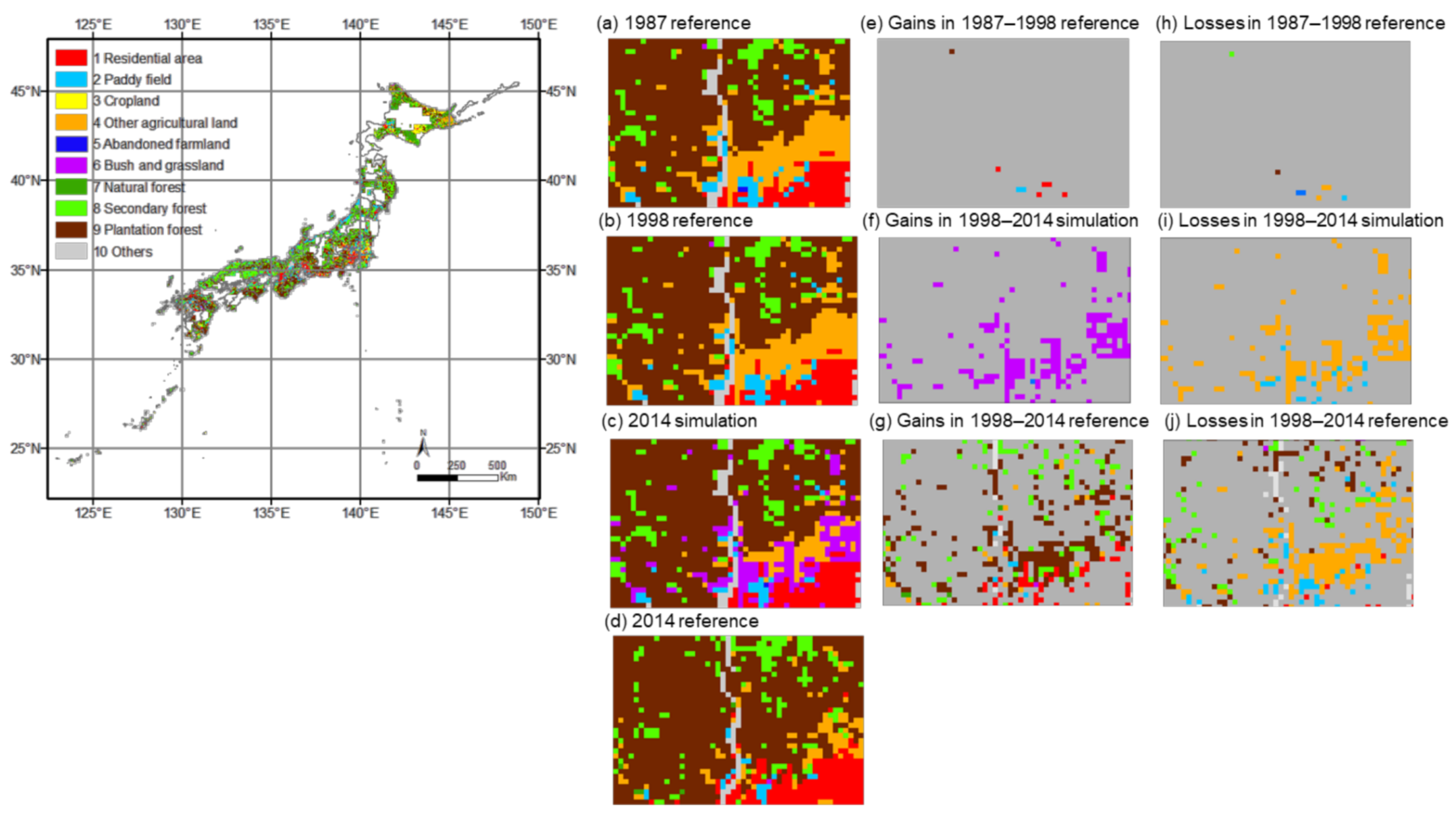
Three types of land change in the BaU scenario were compared to gain insight for the model validation: (1) reference change during the calibration time interval (1987–1998, 11 years), (2) simulation change during 1998–2014 (16 years), and (3) reference change during the validation time interval (1998–2014) (Figure 1). Gains and losses were shown in both the simulation (Figure 1f,i) and validation (Figure 1g,j) periods more than in the calibration time interval (Figure 1e,h). The land-use categories for gains differed between the simulation (Figure 1f) and validation (Figure 1g) periods, but they were similar for losses (Figure 1i,j).

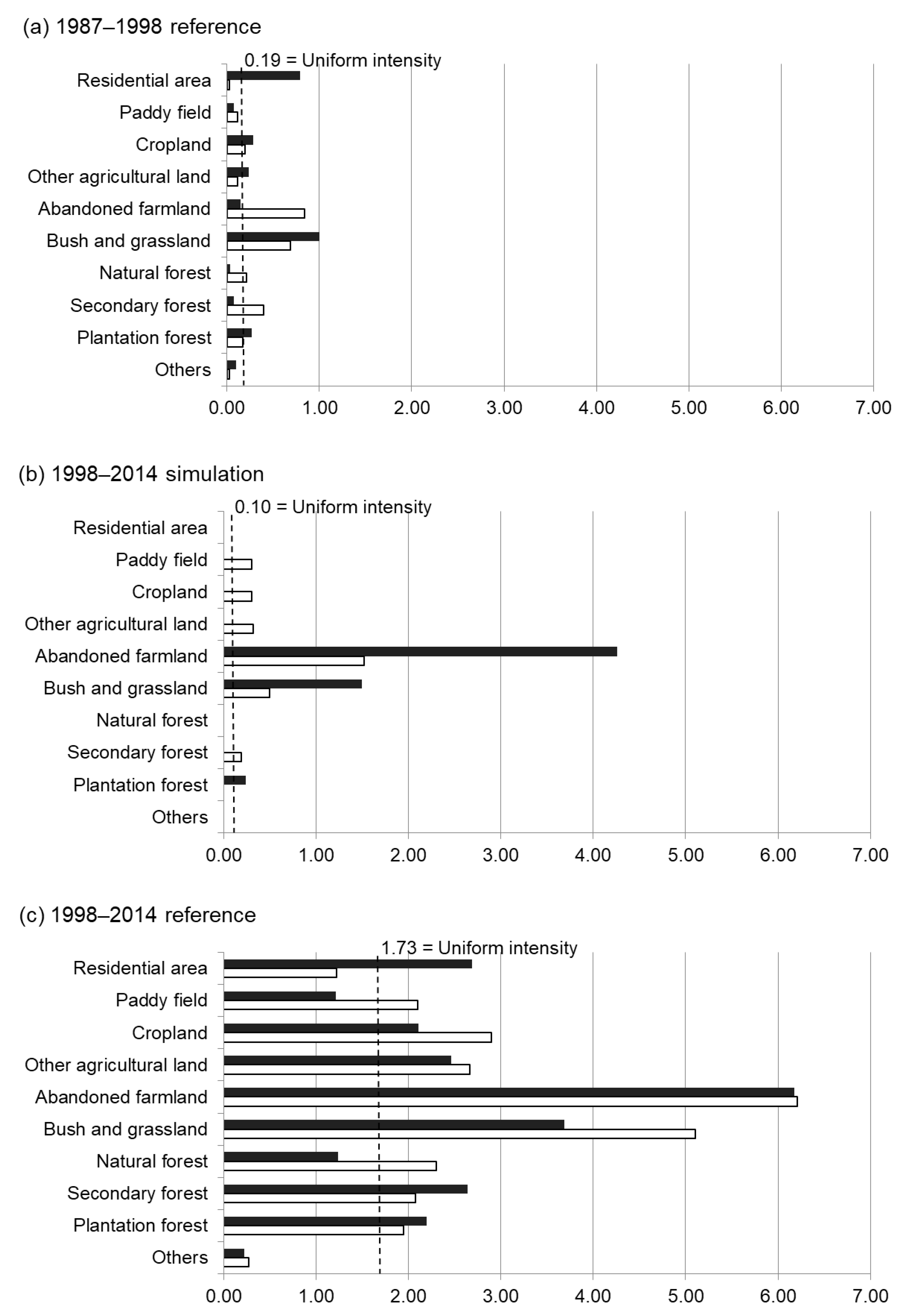
The overall reference change during the calibration time interval was 28,825 cells (2.06% of the spatial extent), the overall simulation change during the validation time interval was 23,292 cells (1.67% of the spatial extent), and the overall reference change during the validation time interval was 385,944 cells (27.7% of the spatial extent) (Appendix A

Table A2. Percent of transition cells from the start time to the end time.

Start Time	End Time										Loss
	Residential Area	Paddy Field	Cropland	Other Agricultural Land	Abandoned Farmland	Bush and Grassland	Natural Forest	Secondary Forest	Plantation Forest	Others
Residential area	4.668	0.001	0.005	0.002	0.000	0.001	0.000	0.001	0.000	0.004	0.01
	5.112	0.000	0.000	0.000	0.000	0.000	0.000	0.000	0.000	0.000	0.000
	4.110	0.263	0.104	0.100	0.001	0.031	0.011	0.240	0.114	0.13	1.002
Paddy field	0.080	9.408	0.007	0.004	0.000	0.002	0.001	0.010	0.008	0.008	0.120
	0.000	9.031	0.000	0.000	0.118	0.341	0.000	0.000	0.000	0.000	0.459
	1.385	6.295	0.319	0.142	0.015	0.028	0.011	0.677	0.522	0.095	3.195
Cropland	0.037	0.006	3.992	0.003	0.000	0.001	0.001	0.017	0.016	0.007	0.088
	0.000	0.000	3.921	0.000	0.000	0.200	0.000	0.000	0.000	0.000	0.200
	0.519	0.284	2.210	0.236	0.006	0.029	0.026	0.411	0.338	0.061	1.911
Other agricultural land	0.020	0.003	0.007	3.245	0.000	0.002	0.000	0.003	0.003	0.005	0.043
	0.000	0.000	0.000	3.163	0.000	0.169	0.000	0.000	0.000	0.000	0.169
	0.255	0.107	0.236	1.910	0.003	0.076	0.070	0.355	0.257	0.063	1.422
Abandoned farmland	0.005	0.000	0.001	0.000	0.072	0.000	0.000	0.000	0.000	0.000	0.007
	0.000	0.000	0.000	0.000	0.055	0.018	0.000	0.000	0.000	0.000	0.018
	0.018	0.004	0.005	0.008	0.000	0.012	0.004	0.011	0.008	0.003	0.072
Bush and grassland	0.024	0.005	0.009	0.012	0.000	2.232	0.005	0.049	0.060	0.018	0.183
	0.000	0.000	0.000	0.000	0.000	2.308	0.000	0.000	0.201	0.000	0.201
	0.077	0.033	0.030	0.115	0.003	0.461	0.347	0.665	0.672	0.106	2.048
Natural forest	0.011	0.002	0.019	0.014	0.000	0.072	10.625	0.011	0.104	0.016	0.248
	0.000	0.000	0.000	0.000	0.000	0.000	10.661	0.000	0.000	0.000	0.000
	0.039	0.018	0.062	0.181	0.001	0.152	6.736	2.393	0.968	0.112	3.925
Secondary forest	0.150	0.04	0.038	0.026	0.000	0.114	0.016	19.933	0.400	0.118	0.908
	0.000	0.000	0.000	0.000	0.000	0.000	0.000	19.466	0.626	0.000	0.626
	0.385	0.443	0.113	0.165	0.003	0.134	0.628	13.405	4.645	0.172	6.687
Plantation forest	0.076	0.019	0.040	0.024	0.000	0.080	0.012	0.060	19.997	0.074	0.385
	0.000	0.000	0.000	0.000	0.000	0.000	0.000	0.000	20.601	0.000	0.000
	0.239	0.291	0.210	0.181	0.003	0.144	0.501	4.733	14.195	0.104	6.406
Others	0.043	0.001	0.003	0.002	0.000	0.003	0.001	0.007	0.013	23.760	0.073
	0.000	0.000	0.000	0.000	0.000	0.000	0.000	0.000	0.000	24.011	0.000
	0.195	0.072	0.048	0.114	0.002	0.057	0.062	0.314	0.171	22.976	1.034
Gain	0.444	0.081	0.128	0.087	0.001	0.277	0.037	0.159	0.604	0.251	2.069
	0.000	0.000	0.000	0.000	0.118	0.728	0.000	0.000	0.826	0.000	1.672
	3.110	1.516	1.127	1.241	0.037	0.663	1.661	9.799	7.695	0.853	27.703

Note: For each transition, the top number shows the 1987–1998 reference, the middle number shows the 1998–2014 simulation, and the bottom number shows the 1998–2014 reference. Bold numbers indicate persistence. Bold italic numbers in the lower right indicate overall change.

). The annual change intensity at the interval level was 0.19% of the spatial extent for the calibration time interval, 0.10% for the simulation change, and 1.73% for the reference change in the validation time interval. Therefore, taking the interval duration into account, the rate of land change was greatest in the reference change during the validation time interval.

Figure 2 shows the results of the category-level intensity analysis. If the intensity was greater than the uniform intensity for a given category, land change was considered to be active; if the intensity was less than the uniform intensity, land change was considered to be dormant. Overall, the transitions simulated in 1998–2014 were more active than those in the 1987–1998 reference group. Losses in agricultural land (paddy, crop, and other agricultural land) changed from dormant to active, and gains in abandoned farmland changed from dormant to active (Figure 2a,b), as shown also in the 1998–2014 reference (Figure 2c). However, the transition status in the simulation change and reference change during 1998–2014 was not consistent, except for losses in agricultural land and secondary forest, gains and losses in abandoned farmland and bush/grassland, and gains in plantation forest. These inconsistencies between the simulation and reference changes should be improved in the simulation model.

Figure 3 shows the results of the transition-level intensity analysis. If the intensity level was greater than the uniform intensity, the transition was considered to be active. If it was less than the uniform intensity, the transition was considered to be dormant. As the land change intensities were larger in the gains of two categories, abandoned farmland and bush/grassland, we focused on those two categories in the figure. The transitions of the two categories were active both in the simulation and the 1998–2014 reference, whereas there was a very little transition in the 1987–1998 reference.

Upon comparing the gains in the simulation and 1998–2014 reference, it can be seen that abandoned farmland targeted only paddy fields in the simulation, but targeted paddy fields, cropland, other agricultural land, and bush/grassland in the reference (Figure 3a). Gains in bush/grassland targeted paddy fields, cropland, other agricultural land, and abandoned farmland in the simulation; paddy fields were not a target in the 1998–2014 reference, but natural forest and plantation forest were to a small extent (Figure 3b). These inconsistencies between the simulation and reference changes should be improved in the simulation model. Specifically, transitions to abandoned farmland from cropland, other agricultural land, and bush/grassland should be involved in the simulation model. Transitions to bush/grassland from paddy fields could be reduced in the simulation model.

3.3. Figure of Merit Components

Table 3. Figure of merit components and correct rejections for the business as usual (BaU) scenario.

Component	Number of Cells
Hits	2314	(0.17)
Misses	373,447	(26.8)
False alarms	20,978	(1.51)
Correct rejections	996,426	(71.52)
Total	1,393,165

Note: Numbers in parentheses indicate the percent of the total.

shows the FOM components and correct rejection for the BaU scenario. Correct rejection, which is the area where the reference persistence is correctly simulated as persistence, was dominant (71.5%), which indicates that the persistence of land use was dominant in this area. Misses (26.8%) was the second largest category, followed by false alarms (1.5%) and hits (0.17%). The FOM was 0.58% (hits as a percentage of the sum of the three components).

The total disagreement (misses plus false alarms) was 28.3%. The quantity disagreement was 25.3%, and the allocation disagreement was 3.0% relative to the spatial extent. These results suggest that the disagreement between the simulation and reference in the validation interval was caused by quantity rather than allocation.

4. Discussion

4.1. Development of Land-Use Scenarios with Limited Data

This study developed finer resolution land-use maps using a GIS-based vegetation database and developed scenarios for estimating plausible future land changes through 2050. The developed scenarios showed notable differences in the future land changes, which policymakers can consider when making decisions about policy options.

GIS-based vegetation maps are a valuable resource to identify detailed land-use categories; however, an important disadvantage is that they are based on field surveys, which are infrequently updated as compared with those created using remote-sensing based techniques. In this study, the latest vegetation data from 2014 were incomplete because of a lack of survey data. Thus, the scenarios used maps from 1987 and 1998 for calibration, and the 2014 map was used for validation only. Finer spatial resolution and updated data are required to detect critical land transitions. The extracted abandoned farmland area was only about 350 km² in the reference map in 1998. Given that currently abandoned farmland accounts for 4230 km² (Census of Agriculture and Forestry, Japan in 2015), transitions relating to abandoned farmland were rarely identified in the map of 500 m resolution. Considering the average cultivated acreage per farm is about 2.4 ha in Japan, a 100 m resolution is required for modeling agricultural land abandonment.

Applying higher spatial and thematic resolution is a fundamental issue in the land-use scenario approach. For example, the CORINE land-cover data, which consist of 44 land cover categories classified using high-resolution satellite imagery, have been used to assess ecosystem services provided by various landscapes in the European Union (EU) [19]. In turn, land system classification to capture the variety of different mosaics of agriculture and forestry was used in Asia [20] rather than biophysical land-cover classification. The classification system is country-specific. However, newer land-use/cover datasets, developed with various sources, such as remote sensing products and GIS-based inventories, enable researchers and practitioners to predict future ecosystem services considering the regional context.

Another issue is how current national scale scenarios could align with climate change scenarios. Specifically, agricultural land use is an important subject in the discourse of climate change impact and adaptation [21]. Climate and population change will affect future land-use changes; however, the impacts might differ depending on the land-use/cover types. In Japan, climate change is likely to have a large impact on croplands, forests, and wastelands, whereas population change may have more influence on paddy fields, built-up areas, and other artificial land covers [22]. PANCES scenarios were used to investigate the impact of plausible policy options for managing natural resources as well as population change [12]. Projecting land-use changes and identifying the potential impacts of various factors can be used to examine the impacts on future human society.

4.2. Scenario Assessment for Communication

Policymakers in Japan have referred to the PANCES land-use scenarios in discussions of the direction of the National Biodiversity Strategy and Action Plan. Regional differences in land changes are particularly important when discussing local strategies at a national scale [12]. The first version of the PANCES scenarios had a resolution of 1 km and showed significant regional differences in susceptible areas that could be influenced by the policy options [7]. However, the scenarios have a low level of accuracy (FOM of 1.56%), which is a concern when choosing policy options. Although communicating the uncertainty of the scenarios is a central issue in any environmental decision-making [9], researchers still must make clear predictions, often based on limited data.

FOM has been used to assess the accuracy of predictions derived from land-use models and to select the best-fit models [23,24,25,26,27]. However, a single metric might not offer sufficient insights as it cannot adequately assess all of the various aspects of modeling [11]. Therefore, this study assessed the developed scenarios by comparing the reference change during a calibration interval, the simulation change, and the reference change during a validation interval.

The reference change during the validation interval had the greatest change intensity (1.7% of the spatial extent) at more than nine times that of the reference change during the calibration interval. This suggests that land changes were overestimated in the 1998–2014 reference map, possibly owing to noise in the vegetation data. National vegetation surveys have been conducted by the Ministry of the Environment of Japan, and GIS-based vegetation maps were created based on the results of the field vegetation surveys. In 1999, however, the survey method changed from guidelines based on a 1:50,000 vegetation map to those based on a 1:25,000 vegetation map [15]. To avoid a mismatch in developing land-use scenarios, the PANCES scenarios used the earlier vegetation data based on the 1:50,000 vegetation map. However, for scenario assessment incorporating the latest land transitions (e.g., transition to abandoned land), the alignment of these spatial data is a primary concern.

Category-level intensity analysis revealed differences in the three types of changes. Although the noise may exist in the 1998–2014 reference group, the intensity of the land change related to gains of abandoned farmland and bush/grassland was apparent in both the simulation and reference validation groups (Figure 2). The transition-level analysis showed which land-use categories were targeted by abandoned farmland and bush/grassland (Figure 3). Gains in abandoned farmland targeted only paddy fields in the simulation, whereas all types of agricultural land and bush/grassland were targeted in the 1998–2014 reference group. Modeling could be improved to reduce this kind of mismatch using the appropriate map for validation.

Quantity disagreement was observed to be more important than allocation disagreement in the BaU scenario in the simulation as compared with the 1998–2014 reference validation (Section 3.3). This suggests the model could be improved by setting the amount of future land-use demand first and then assessing the model to check for any allocation disagreement. As information regarding the spatial distribution of land use is important in the National Biodiversity Strategy and Action Plan, measuring the allocation disagreement should also be considered in the assessment of land-use scenarios.

5. Conclusions

This study conducted scenario assessment using land-use maps of 500 m spatial resolution derived from vegetation inventory data at the national scale. The study revealed the potential causes for low accuracy of the national scale land-use scenarios (noises in reference maps and inappropriate transitions in the simulation model) as well as priority solutions, such as the alignment of spatial vegetation maps and model improvement, in order to reduce the two types of disagreement between the simulation and reference maps. In the field of land-use modeling for environmental decisions, dynamic land changes, such as rapid urban development and the reduction of natural vegetation, have been modeled to reveal the impacts of land-use policy on ecosystems. This is particularly valid in Asia, where population expansion and economic development are major factors affecting biodiversity and ecosystem services. However, depopulation will pose new problems in the near future. Developing plausible scenarios using limited information remains a challenge, and further research is needed for the scenario assessment of various aspects of model outputs. The updated scenarios enable us to identify trade-offs and synergies between sustainable development goals.

References

- Verburg, P.H.; Schot, P.P.; Dijst, M.J.; Veldkamp, A. Land use change modelling: Current practice and research priorities. Geo J. 2004, 61, 309–324. [Google Scholar] [CrossRef]
- IPBES. The Methodological Assessment Report on Scenarios and Models of Biodiversity and Ecosystem Services; Secretariat of the Intergovernmental Science-Policy Platform on Biodiversity and Ecosystem Services: Bonn, Germany, 2016; ISBN 9789280735697. [Google Scholar]
- Sitas, N.; Harmáčková, Z.V.; Anticamara, J.A.; Arneth, A.; Badola, R.; Biggs, R.; Blanchard, R.; Brotons, L.; Cantele, M.; Coetzer, K.; et al. Exploring the usefulness of scenario archetypes in science-policy processes: Experience across IPBES assessments. Ecol. Soc. 2019, 24, 35. [Google Scholar] [CrossRef]
- Saito, O.; Kamiyama, C.; Hashimoto, S.; Matsui, T.; Shoyama, K.; Kabaya, K.; Uetake, T.; Taki, H.; Ishikawa, Y.; Matsushita, K.; et al. Co-design of national-scale future scenarios in Japan to predict and assess natural capital and ecosystem services. Sustain. Sci. 2019, 14, 5–21. [Google Scholar] [CrossRef]
- Matsui, T.; Haga, C.; Saito, O.; Hashimoto, S. Spatially explicit residential and working population assumptions for projecting and assessing natural capital and ecosystem services in Japan. Sustain. Sci. 2019, 14, 23–37. [Google Scholar] [CrossRef]
- Hori, K.; Saito, O.; Hashimoto, S.; Matsui, T.; Akter, R.; Takeuchi, K. Projecting population distribution under depopulation conditions in Japan: Scenario analysis for future socio-ecological systems. Sustain. Sci. 2021, 16, 295–311. [Google Scholar] [CrossRef] [PubMed]
- Shoyama, K.; Matsui, T.; Hashimoto, S.; Kabaya, K.; Oono, A.; Saito, O. Development of land-use scenarios using vegetation inventories in Japan. Sustain. Sci. 2019, 14, 39–52. [Google Scholar] [CrossRef]
- Perpiña Castillo, C.; Jacobs-Crisioni, C.; Diogo, V.; Lavalle, C. Modelling agricultural land abandonment in a fine spatial resolution multi-level land-use model: An application for the EU. Environ. Model. Softw. 2021, 136, 104946. [Google Scholar] [CrossRef] [PubMed]
- Manski, C.F. Communicating uncertainty in policy analysis. Proc. Natl. Acad. Sci. USA 2019, 116, 7634–7641. [Google Scholar] [CrossRef] [Green Version]
- Eastman, J.R. TerrSet Tutorial: Geospatial Monitoring and Modeling System; Clark Labs: Clark University, Worcester, MA, USA, 2016. [Google Scholar]
- Varga, O.G.; Pontius, R.G.; Singh, S.K.; Szabó, S. Intensity analysis and the figure of merit’s components for assessment of a cellular automata—Markov simulation model. Ecol. Indic. 2019, 101, 933–942. [Google Scholar] [CrossRef]
- Saito, O.; Hashimoto, S.; Kabaya, K.; Hori, K.; Matsui, T.; Haga, C.; Shoyama, K.; Kameyama, Y.; Takahashi, Y.; Yamazaki, M.; et al. Future Scenarios and Integrated Model of Social-Ecological Systems on National and Regional Scales. PANCES Policy Brief 2020, 1–12. [Google Scholar]
- Ogawa, M.; Takenaka, A.; Kadoya, T.; Ishihama, F.; Yamano, H.; Akasaka, M. A comprehensive new land-use classification map for Japan for biodiversity assessment and species distribution modeling. Jpn. J. Conserv. Ecol. 2013, 18, 69–76. [Google Scholar] [CrossRef]
- Akasaka, M.; Takenaka, A.; Ishihama, F.; Kadoya, T.; Ogawa, M.; Osawa, T.; Yamakita, T.; Tagane, S.; Ishii, R.; Nagai, S.; et al. Development of a National Land-Use/Cover Dataset to Estimate Biodiversity and Ecosystem Services. In Asia-Pacific Biodiversity Observation Network: Integrative Observations and Assessments; Nakano, S., Yahara, T., Nakashizuka, T., Eds.; Springer: Tokyo, Japan, 2014; ISBN 978-4-431-54782-2. [Google Scholar]
- Ogawa, M.; Mastuzaki, S.; Ishihama, F. Explanation of a comprehensive land-use classification map of Japan based on the latest 1:25,000 vegetation map by the Ministry of the Environment. Jpn. J. Conserv. Ecol. 2020, 25, 117–122. [Google Scholar]
- Aldwaik, S.Z.; Pontius, R.G. Intensity analysis to unify measurements of size and stationarity of land changes by interval, category, and transition. Landsc. Urban Plan. 2012, 106, 103–114. [Google Scholar] [CrossRef]
- Aldwaik, S.Z.; Pontius, R.G. Map errors that could account for deviations from a uniform intensity of land change. Int. J. Geogr. Inf. Sci. 2013, 27, 1717–1739. [Google Scholar] [CrossRef]
- Pontius, R.G.; Boersma, W.; Castella, J.C.; Clarke, K.; Nijs, T.; Dietzel, C.; Duan, Z.; Fotsing, E.; Goldstein, N.; Kok, K.; et al. Comparing the input, output, and validation maps for several models of land change. Ann. Reg. Sci. 2008, 42, 11–37. [Google Scholar] [CrossRef] [Green Version]
- Cole, B.; Smith, G.; Balzter, H. Acceleration and fragmentation of CORINE land cover changes in the United Kingdom from 2006–2012 detected by Copernicus IMAGE2012 satellite data. Int. J. Appl. Earth Obs. Geoinf. 2018, 73, 107–122. [Google Scholar] [CrossRef]
- Ornetsmüller, C.; Verburg, P.H.; Heinimann, A. Scenarios of land system change in the Lao PDR: Transitions in response to alternative demands on goods and services provided by the land. Appl. Geogr. 2016, 75, 1–11. [Google Scholar] [CrossRef] [Green Version]
- IPCC. Climate Change 2014 Part A: Global and Sectoral Aspects; Cambridge University Press: Cambridge, UK, 2014; ISBN 9781107641655. [Google Scholar]
- Fujita, T.; Ariga, T.; Ohashi, H.; Hijioka, Y.; Fukasawa, K. Assessing the potential impacts of climate and population change on land-use changes projected to 2100 in Japan. Clim. Res. 2019, 79, 139–149. [Google Scholar] [CrossRef]
- Subasinghe, S.; Estoque, R.C.; Murayama, Y. Spatiotemporal analysis of urban growth using GIS and remote sensing: A case study of the colombo metropolitan area, Sri Lanka. ISPRS Int. J. Geo-Inf. 2016, 5, 197. [Google Scholar] [CrossRef] [Green Version]
- Pontius, R.G.; Thontteh, O.; Chen, H. Components of information for multiple resolution comparison between maps that share a real variable. Environ. Ecol. Stat. 2008, 15, 111–142. [Google Scholar] [CrossRef]
- Li, X.; Chen, G.; Liu, X.; Liang, X.; Wang, S. A new global land-use and land-cover change product at a 1-km resolution for 2010 to 2100 based on human—environment interactions. Ann. Am. Assoc. Geogr. 2017, 107, 1040–1059. [Google Scholar] [CrossRef]
- Cao, M.; Zhu, Y.; Quan, J.; Zhou, S.; Lü, G.; Chen, M. Spatial sequential modeling and predication of global land use and land cover changes by integrating a global change assessment model and cellular automata Earth’s future. Geophys. Res. Lett. 2019, 46, 8329–8337. [Google Scholar] [CrossRef] [Green Version]
- Thapa, R.B.; Murayama, Y. Urban Growth Modeling Using the Bayesian Probability Function. In Progress in Geospatial Analysis; Murayama, Y., Ed.; Springer: Tokyo, Japan, 2012. [Google Scholar]
Figure 1.
Entire land-use map in 2014 (left) and examples of reference maps and changes during two time intervals: reference map in 1987 (a); reference map in 1998 (b); simulation map in 2014 (c); reference map in 2014 (d); and gains (e–g) and losses (h–j) of each land use category during the calibration (1987–1998), simulation (1998–2014), and validation (1998–2014) time intervals. Each color shows the changes in land-use, and the grey color shows persistence, which indicates that a land-use category remained the same during a time interval (e–j).
Figure 2.
Category intensities for the (a) 1987–1998 reference (calibration), (b) 1998–2014 simulation, and (c) 1998–2014 reference (validation) intervals. Black bars show the gain intensity and white bars show the loss intensity. The vertical dashed line shows uniform intensity.
Figure 3.
Transition intensities for the gains of (a) abandoned farmland and (b) bush and grassland for the 1987–1998 reference (calibration), 1998–2014 simulation, and 1998–2014 reference (validation) intervals. Black bars show active transitions and grey bars show dormant transitions. The vertical dashed line shows uniform intensity.