
The Importance of Low-Intensive Agricultural Landscape for Birds of Prey


1
Marine Biological Station “Prof. Dr. Ioan Borcea”, Agigea, “Alexandru Ioan Cuza” University of Iași, B-dul Carol I, No. 20A, 700506 Iași, Romania
2
Romanian Ornithological Society/BirdLife Romania, B-dul Hristo Botev, nr. 3/6, 030231 Bucharest, Romania
3
Center for the Study of Transborder and Emergent Diseases and Zoonoses, Danube Delta National Institute for Research and Development, Babadag Street, nr. 165, 820112 Tulcea, Romania
4
Faculty of Biology, “Alexandru Ioan Cuza” University of Iași, B-dul Carol I, No. 20A, 700506 Iași, Romania
*
Author to whom correspondence should be addressed.
Land 2021, 10(3), 252; https://doi.org/10.3390/land10030252
Submission received: 11 January 2021
/
Revised: 14 February 2021
/
Accepted: 25 February 2021
/
Published: 2 March 2021
(This article belongs to the Collection Land Systems in Transition: Challenges, Approaches, and Pathways for a Sustainable Development)
Abstract
:Low-intensive agricultural areas of Romania sustain high species diversity. Together with natural habitats, these areas are very important for European biodiversity. The ecosystem´s health is reflected in the predator status because of their position at the top of the trophic networks. The Common Buzzard (Buteo buteo) is the most common bird of prey species in Europe. During the first survey census conducted in Eastern Romania (2011–2012 breeding seasons), 8.55–10.35 breeding pairs/100 square km have been counted. The Common Buzzard density varies between breeding seasons and with differences in habitat structure. Their density is positively influenced by the density of forest edge and Simpson diversity index of habitats but is negatively influenced by the total habitat fragmentation and mean daily temperature. According to this analysis, the selection of breeding territories by common buzzards is positively influenced by a heterogeneous landscape in an area with low-intensive agriculture and with large areas of open habitats made up of natural or semi-natural vegetation.
1. Introduction
Understanding the mechanisms involved in the distribution and abundance of an organism is the fundamental goal of ecology [1,2]. These mechanisms can be used for successful conservation and restoration strategies in the face of an anthropogenic biodiversity crisis that threatens many of the world’s species [3]. The abundance and presence of a particular bird species may reflect the ecological value of an area [4]. Top predators are a group of species that reflect an area’s biodiversity richness, acting as indicators [5]. They may directly cause high biodiversity, and they may be spatio-temporally associated with it [6].
Today, European biodiversity depends on a large proportion of habitat provided by low-intensity farming practices, a resource that is declining as European agriculture becomes more intensive [7]. After the Iron Curtain fell, Eastern Europe began to develop, leading to intensive agriculture and the aggressive management of habitats. However, development was slow and patchy, so a low-intensive agriculture system still exists, with a landscape comprising a mix of natural and semi-natural vegetation across large areas. This slow landscape development and presence of low intensive agriculture is conducive to high biodiversity in Eastern Europe [8].
The biodiversity richness declined with increasing land-use intensity [9]. Low-intensity farming ensures high conservation values, through a heterogeneous mosaic of crops and providing many different, well-connected structures, such as field edges and roadside vegetation [10]. The small amount of fertilizers used in this type of agriculture supports higher biodiversity richness [9,10,11]. This evidence suggests that species richness can be increased by changing the agricultural practice to low-intensity land use [12].
Birds of prey represent a group of animals highly studied in Western Europe due to their importance for biodiversity and their impressive features. However, they are poorly studied in Eastern Europe where there are fewer ornithologists and species’ distribution studies still require more detailed surveys and research. For this region of Europe, there are many question marks regarding raptor ecology.
The Common Buzzard (Buteo buteo) is a medium size top predator which inhabits Europe and parts of Asia and Africa [13]. As one of the most common bird of prey species in Europe [14], the Common Buzzard could be used as a model of distribution and interaction with biotic and abiotic factors for those top predators which use agricultural areas for hunting. The species’ breeding area characteristics, nesting in trees and foraging opportunistically in an open or semi-open landscape, are linked with all habitat categories [13]. These characteristics turn the Common Buzzard into a bioindicator species for ecosystem health and landscape diversity.
The population density and distribution of a species could be affected by various landscape, geomorphological, and climatic factors [15,16,17,18]. Bird species select habitat patches which suit their primary requirements, such as breeding and foraging [2], making the landscape structure an important factor for bird of prey density and breeding success [19]. Geomorphological features could influence where the nest is located [20], alongside natural variation in the choice of nest site the species makes, especially in areas with heterogeneous landscape features [21]. Climatic factors influence not only the breeding but also the wintering populations due to the species’ physiological limits [22] and could affect the breeding success through extreme weather conditions [23].
Low-intensive agriculture could influence the breeding ecology of raptors. This raises the question of whether landscape features are more important than climatic or geomorphological ones. How does the common buzzard interact within different habitat structures that have a large proportion of natural or semi-natural habitat vegetation patches? To clarify these ecological aspects, our study aims to: (1) Calculate the density of the Common Buzzard population in Eastern Romania, (2) analyze the common buzzard’s distribution in relation to landscape structure, geomorphological and climatic variables. This will be conducted in an area where this species is studied for the first time on such a large scale in Eastern Europe.
2. Materials and Methods
2.1. Study Area
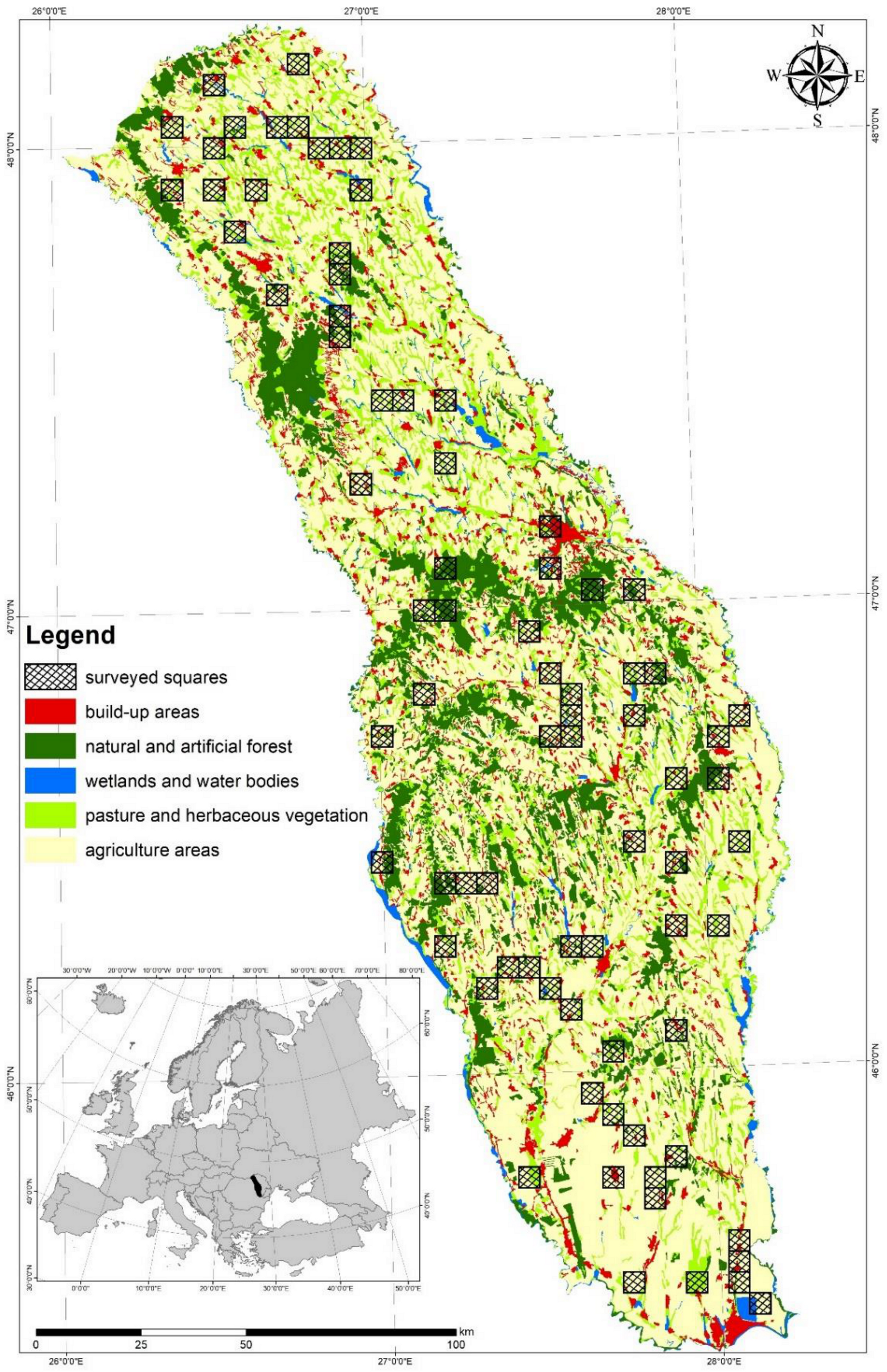
The study area covers the eastern part of the Moldova Region (46°55′ N, 27°11′ E), between the Siret and Prut rivers (land area 22,465.3 km2) in Romania. In general, this is a hilly region (mean elevation 288.6 m) with a mosaic of natural, semi-natural, and artificial habitats [24]. The dominant habitat in the study area is the arable land (51%), which is managed using low-intensive agricultural practices. The most common agricultural crops are: Maize, wheat, potatoes, sunflower, and barley [25]. Habitat coverage in the study area for pasture and herbaceous vegetation is 14.52% and for natural and artificial forest, it is 3.84%. The pasture and herbaceous areas cover mostly the river valleys and are used for grazing and mowing by the local communities. The natural and artificial forests are concentrated in the central and north-western parts of the study area (Figure 1). Most of the artificial forests are small plantations of black locust (Robinia pseudoacacia) and coniferous trees (especially Black Pine (Pinus nigra) and Scots Pine (Pinus sylvestris)). The other habitat types are poorly represented: Agriculture mixed with significant natural vegetation (7.46%), build-up areas (6.89%), vineyards (3.23%), wetlands and waterbodies (2.03%), and orchards (1.03%).
2.2. Study Design and Buzzard Data Collection
The entire study area was covered by a 5 × 5 km grid using Hawths Tools, v.3.x extension for Arc GIS v.9.3. Using the Create Random Selection Tool from the same extension, 80 observation squares summing 2000 square km (8.9% from the study area) were selected. The condition used during this random selection process was to have similar habitat proportions in the surveyed squares as in the study area. Using satellite images and relief maps, we selected between four and eight observation points for each surveyed square, according to the habitat composition and terrain structure. The observation points were manually selected to be at good vantage points so that as much of the area as possible could be seen so as to have a full observation coverage for each square.
The field observations were conducted during two breeding seasons (2011–2012). In each season, we conducted one field observation at each observation point. Considering that Common Buzzard is an early breeder in Eastern Romania [22], the field period ranged from 15 April to 15 June. The field observations were conducted between 09.00 A.M. and 18.00 P.M. Each observation period lasted 2 h, in which the observers searched actively for birds of prey. Each square was covered by three to five experienced ornithologists at different points. To avoid double counting, the observers communicated the position for each bird of prey using mobile phones and walkie-talkie devices. If a bird was observed from two points, it was recorded only by the observer who was able to identify the possible nest location.
During the observations, all birds of prey species were recorded. For each individual, we recorded the age class, sex (if it was possible), the observation time, and the behavior. The last one being used to evaluate their breeding status and calculate the number of breeding pairs (for detailed information, see [17,22]). The observer tried to identify the possible nest location (the area where the bird enters the forest repeatedly) and locate it on a map. All the observations were integrated into an ArcGIS database, using the marked location for each bird of prey. Over both breeding seasons, 13 breeding species and four non-breeding species of bird of prey were recorded (Appendix A).
The present survey method was designed to collect data on the Common Buzzard and the Long-legged Buzzard as the main species and to also record other birds of prey that breed or forage in the surveyed areas. Because our observations started early, in mid-April, we excluded results for other bird of prey species except for Sparrowhawk (Accipiter nisus) and Northern Goshawk (Accipiter gentilis). Their breeding period is covered by the study period, although there are different and more effective methods for recording these two species. Our method can include the Long-legged Buzzard as it has been designed to also include observation points in areas without forest patches inhabited by this species. This is a species that is expanding its breeding and wintering range [22,26,27]. Due to its low abundance in our study area (eight pairs in the first season and five in the second), we were unable to analyze the distribution or territory selection for this species in the present study. Due to these drawbacks, only the data on Common Buzzard for studying the species breeding distribution and territory selection were analyzed.
2.3. Environmental and Climatic Predictor Variables
To analyze the influence of landscape and climatic variables on the breeding population of Common Buzzard in Eastern Romania, we recorded data for 22 variables (Table 1) from two main perspectives, the quantitative and the matrix composition [2]. The quantitative perspective contains relief, climatic data, and habitat proportion for each surveyed square, which are separated into eight variables (habitat category). The matrix composition perspective covers not only the habitat type, but also the relation between two or more habitats, including edge influence, which includes total ecotone length, total forest edge, ecotone length/number of habitat patch, and forest edge/number of forest patch, habitat patch structure, which includes the number of habitat patches and the number of forest patches, relief structure which includes mean altitude, altitude standard deviation and altitude variability and habitat diversity indexes, such as the Shannon Index, the Shannon Equitability and the Simpson Index).
For habitat data, we used Corine land-cover maps (1:100,000). The habitats were separated into eight categories (Table 1) and were integrated into the analyses as habitat cover (in %) for each surveyed square. The edge influence variables were extracted from Corine land-cover maps using two approaches. Habitat edge or ecotone area represent the place where two habitats (or more) came in contact. These areas are important for small animals because they can find a place of refuge but also for birds of prey that hunt near them. The first one involves all habitats from each surveyed square (total ecotone length in a 5 × 5 km square), and the second one involved only the natural and artificial forest edge (in a 5 × 5 km square). The natural and artificial forest edges were considered due to their importance in nest selection by Common Buzzards [26]. Additionally, we calculated the edge density as the edge length divided by the number of forests [28]. The habitat patch structure was recorded as the total number of individual habitat patches. For each surveyed square, we also calculated the Shannon Index, the Shannon Equitability and the Simpson Index using Landcover Analysis (LecoS) plugin for Quantum GIS v. 2.14.11. Essen [28].
The relief structure variables were extracted from SRTM 90 m Digital Elevation Model Dataset [29]. For each 5 × 5 surveyed square, three variables were calculated: The mean altitude, standard deviation (of all cells from the 5 × 5 km square), and variability (the number of unique values for all cells in a 5 × 5 km squares).
The climatic variables were calculated as a mean value for each 5 × 5 km surveyed square. Using WorldClim information [30], two climatic variables were built: Mean daily temperature and annual precipitations (Table 1).
In addition to the landscape, geomorphological and climatic variables, we also added, in the Generalized Linear Mixed Model (GLMM) analysis, the number of all bird of prey species that breed in the study area. For all other birds of prey (except Common Buzzards), we recorded only the number of individuals without calculating the breeding pairs due to their different breeding periods. Most of the birds of prey do not breed as early as Common Buzzard.
2.4. Data Analyses
A GLMM approach was used to determine the influence of landscape, geomorphological, and climatic variables on the Common Buzzard’s breeding abundance in Eastern Romania. For this analysis, we used the total number of breeding pairs of Common Buzzards for each of the 80 surveyed squares during two breeding seasons (n = 160). Because the data of breeding Common Buzzards came from 80 surveyed squares from two breeding seasons, we included surveyed squares and breeding seasons as random effects. Using this response variable (number of Common Buzzard breeding pairs), the model employed a Negative Binomial error structure and log link function. In the first step, we performed full models that included all landscape and climatic variables. We excluded least-significant variables in a stepwise procedure, using Akaike‘s Information Criterion (AIC) to select the best model (Table 2). This model evaluation was done using the all possible subsets method with “MuMIn” package for R statistical software v.3.2. To evaluate the model adequacy, the residuals versus fitted values and explanatory variables were plotted, but no distinct patterns were observed. Moreover, the model multicollinearity effects were tested using VIF (Variance Inflation Factors) function from the “car” package. For our selected model, we get VIF value lower than 2, indicating that our variables are not correlated. The analysis was conducted in R statistical software v.3.2 [31] with “glmmADMB” package.
3. Results
The main target species, the Common Buzzard, was the most common bird of prey across the study area. Their number was not similar during these two breeding seasons. For the first year, we counted 207 pairs, and for the second year, 171 pairs. The relative density was higher in the first season when we recorded 10.35 breeding pairs/100 km2 than in the second season when we counted 8.55 breeding pairs/100 km2. The variability was also recorded across the surveyed squares, from 0–14 breeding pairs/5 × 5 square in the first season and 0–10 breeding pairs/5 × 5 square in the second season.
To better understand the Common Buzzard’s breeding territory selection, we conducted a GLMM analysis. During the first step of the analysis, alongside the landscape and climatic factors, we also included the other breeding bird of prey species that were recorded during the field surveys (Appendix A). From these, only the Northern Goshawk had a significant positive influence on the Common Buzzard, but this species was excluded from the GLMM analysis after we tested for multicollinearity. This bird of prey species was correlated with the same landscape variable as the Common Buzzard.
The best GLMM model includes six out of 22 landscape and climatic variables (Table 2). Except for the forest coverage, which was not present in one model, the other variables were included in the final top five models.
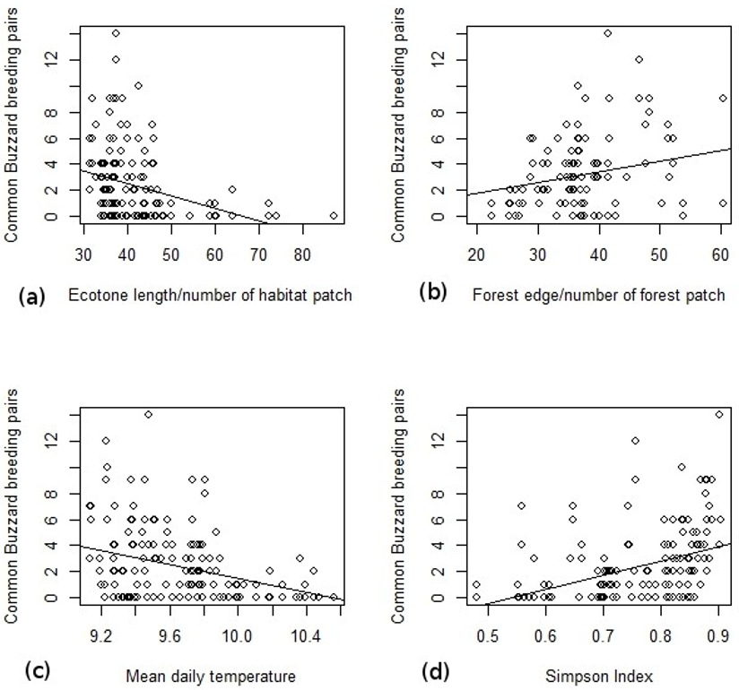
According to the GLMM analysis, the Common Buzzard’s distribution is positively influenced by forest edge density (Z = 3.17, p = 0.002) and Simpson Index (Z = 2.41, p = 0.16), and negatively influenced by the total habitat fragmentation (Z = −2.54, p = 0.011) and mean daily temperature (Z = −3.13, p = 0.016, Table 3, Figure 2). There are no geomorphological variables which influence the Common Buzzard’s breeding abundance. Regarding the climatic variable, the final model includes mean daily temperature that influences the breeding abundance of Common Buzzards. A lower daily mean temperature is associated with a higher Common Buzzard abundance. Forest coverage and altitude variation are included in the final GLMM but without a significant influence on the Common Buzzard’s abundance.
4. Discussion
The Common Buzzard’s relative mean density looks smaller than that of other populations from Eastern Europe (e.g., Central Poland—17.3 breeding pairs/100 km2, [20]), but is similar with nesting density from the Apennines mountain areas [32]. However, a comparison with these studies is almost impossible because the study area which they covered is quite small (e.g., [33,34]). Our study covers large areas, including regions with a high percentage of open habitats, unsuitable for the species to breed. The Common Buzzard’s density varies across the study area, from zero breeding pairs/surveyed square to a maximum of 14 breeding pairs/surveyed squares. The lowest limit was recorded in those surveyed squares without forest patches. These data suggest that, in the study area, the Common Buzzard is dependent on forests for nest location. Large arable fields without forest patches did not ensure suitable sites for breeding Common Buzzards. This was because in the study area, it does not breed in tree lines or small groups of trees [35] as it breeds in the other regions from Western Europe [36].
The positive influence of Northern Goshawks on the Common Buzzard’s abundance, which was revealed in the first stage of the GLMM analyses, is not in accordance with other studies from Europe (e.g., [37,38,39]) and from Romania [35], which show that these two birds of prey species are in competition. However, in the study area, these two species have a slightly different nesting area selection. Northern Goshawks use mostly areas close to human settlements. Aside from this reference, they use a similar habitat structure [35]. These approaches explain the multicollinearity relation, which was identified in our first GLMM analyses, for which it was needed to exclude the variables on the other bird of prey species.
Habitat composition is important for the Common Buzzard’s breeding preferences due to their nesting and foraging territories requirements [40,41]. The landscape structure (habitat cover) did not explain the Common Buzzard’s abundance, although their connectivity measures tend to explain the variation in species’ distribution [2]. These landscape factors which have a significant influence on the Common Buzzard’s breeding territory selection relate to habitat diversity and structure. Forest-dwelling birds of prey are linked to large-scale landscape composition and with better breeding success in areas with high coverage of forest [19,42,43]. Our analyses revealed that patches of forests should have a direct effect on increasing the Common Buzzard’s population, offering nesting places and shorter distances to their foraging grounds. Similar results were found in France, where hedgerows and woodlots are highly important for the abundance of the Common Buzzard [44], due to their use as breeding places. Habitat diversity, through the Simpson Index, is another important landscape variable with a significant positive influence on the Common Buzzard’s abundance. An area with a high Simpson Index offers a large variety of foraging sites, ensuring higher prey diversity for the Common Buzzard [44]. The Goshawk population size is also positively influenced by habitat heterogeneity, even if this species is strongly related with closed habitats [45]. However, the landscape composition should not be highly fragmented because this variable is associated with a low Common Buzzard abundance. Highly fragmented habitats were found to be an important variable for decreasing the abundance of Common Buzzards in France too [44]. An area with high forest density and habitat diversity but with low habitat fragmentation and mean daily temperature will ensure ideal breeding conditions for Common Buzzards in Eastern Romania.
The geomorphological variables did not influence the Common Buzzard’s distribution, probably because the relief is quite uniform in the study area, especially if we calculate the variables for a grid of 5 × 5 square km. This type of variable is more important for those raptor species which breed on cliffs but less important for tree specialist birds [13].
The influence of mean daily temperature on the Common Buzzard’s breeding abundance is the opposite of another study conducted in Finland [46]. However, this analysis could also be influenced by the temperature segregation in the study area, which is conducted by geographic features from the study area. The southern part of the study area shows higher temperatures, but this region is less suitable for Common Buzzards due to very small, or even without forest patches, being covered mainly by open habitat. The middle and the northern part of the study area have larger forest patches ensuring good nesting opportunities.
Due to this opportunistic behavior regarding the food supply, we did not include food density in the analyses. If the variety of prey is large, the Common Buzzard’s density cannot be influenced by these variables [45,47], especially in areas with high biodiversity, as in Eastern Europe.
This study presents the first data on the Common Buzzard’s breeding abundance and its relationship with the landscape and geomorphological and climatic features. The analyses show the positive influence of a heterogeneous landscape on the Common Buzzard’s breeding territory selection from an area with low-intensive agriculture and with large surfaces of open habitats crossed by natural or semi-natural vegetation elements. The presence of natural or semi-natural elements across the agricultural fields is in accordance with the European Regulations [48]. These results can contribute to species conservation at a regional scale, and inform environmentally friendly agricultural practices, for example, using Common Buzzards to control the rodent populations from the arable land.
5. Conclusions
The patches of forests have a direct effect on increasing the Common Buzzard’s population, offering nesting places and shorter distances to their foraging grounds. An area with high forest density and habitat diversity but with low habitat fragmentation and mean daily temperature will ensure ideal breeding conditions for Common Buzzards in Eastern Romania.
The heterogeneous landscape has a positive influence on the Common Buzzard’s breeding territory selection from an area with low-intensive agriculture and with large surfaces of open habitats crossed by natural or semi-natural vegetation elements.
Author Contributions
E.Ș.B.—Study conception, Methodology, Formal analysis, Investigation: data/evidence collection, Writing/manuscript preparation: writing the initial draft. V.P.—Investigation: data/evidence collection; L.E.B.—Investigation: data/evidence collection; C.I.—Investigation: data/evidence collection. All authors have read and agreed to the published version of the manuscript.
Funding
This research received no external funding.
Institutional Review Board Statement
Not applicable.
Informed Consent Statement
Not applicable.
Data Availability Statement
Data available on request from the authors.
Acknowledgments
We wish to thank to Ed Drewitt, Andrei Ştefan, Laurenţiu Petrencu and reviewers for their improvements on a previous version of this manuscript.
Conflicts of Interest
The authors declare no conflict of interest.
Appendix A

Table A1.
The total number of birds of prey and owl species recorded during 2011 and 2012 breeding seasons in eastern Romania.
Table A1.
The total number of birds of prey and owl species recorded during 2011 and 2012 breeding seasons in eastern Romania.
| No. crt. | English Name | Scientific Name | Individuals/Breeding Season | |
|---|---|---|---|---|
| 2011 | 2012 | |||
| Breeding bird of prey species | ||||
| 1 | Northern Goshawk | Accipiter gentilis | 27 | 19 |
| 2 | Sparrowhawk | Accipiter nisus | 1 | 1 |
| 3 | Booted Eagle | Aquila pennata | 2 | 1 |
| 4 | Lesser Spotted Eagle | Aquila pomarine | 19 | 8 |
| 5 | Common Buzzard | Buteo buteo * | 207 | 171 |
| 6 | Long-legged Buzzard | Buteo rufinus * | 8 | 5 |
| 7 | Short-toed Eagle | Circaetus gallicus | 0 | 1 |
| 8 | Marsh Harrier | Circus aeruginosus | 29 | 31 |
| 9 | Hobby | Falco subbuteo | 5 | 6 |
| 10 | Kestrel | Falco tinnunculus | 80 | 38 |
| 11 | Red-footed Falcon | Falco vespertinus | 12 | 36 |
| 12 | Black Kite | Milvus migrans | 1 | 0 |
| 13 | Honey Buzzard | Pernis apivorus | 32 | 31 |
| Non-breeding bird of prey species | ||||
| 14 | Steppe Eagle | Aquila heliaca | 0 | 2 |
| 15 | Hen Harrier | Circus cyaneus | 4 | 0 |
| 16 | Montagu’s Harrier | Circus pygargus | 1 | 1 |
| 17 | Saker Falcon | Falco cherrug | 0 | 1 |
| Owl species | ||||
| 18 | Little Owl | Athene noctua | 1 | 0 |
| 19 | Tawny Owl | Strix aluco | 1 | 0 |
For Common Buzzards (*) and Long-legged Buzzards (*) pair numbers were recorded and for other species we counted the total number of individuals observed.
References
- Begon, M.; Harper, J.L.; Townsend, C.R. Ecology: Individuals, Populations and Communities; Blackwell Science Ltd.: Oxford, UK, 1996. [Google Scholar]
- Watling, J.I.; Nowakowski, A.J.; Donnelly, M.A.; Orrock, J.L. Meta-analysis reveals the importance of matrix composition for animals in fragmented habitat. Glob. Ecol. Biogeogr. 2010, 20, 209–217. [Google Scholar] [CrossRef]
- Ehrlich, P.R.; Pringle, R.M. Where does biodiversity go from here? A grim business-as-usual forecast and a hopeful portfolio of partial solutions. Proc. Natl. Acad. Sci. USA 2008, 105, 11579–11586. [Google Scholar] [CrossRef] [Green Version]
- Gilroy, J.J.; Anderson, G.Q.; Grice, P.V.; Vickery, J.A.; Bray, I.; Watts, P.N.; Sutherland, W.J. Could soil degradation contribute to farmland bird declines? Links between soil penetrability and the abundance of yellow wagtails Motacilla flava in arable fields. Biol. Conserv. 2008, 141, 3116–3126. [Google Scholar] [CrossRef]
- Billeter, R.; Liira, J.; Bailey, D.; Bugter, R.; Arens, P.; Augenstein, I.; Aviron, S.; Baudry, J.; Bukacek, R.; Burel, F.; et al. Indica-tors for biodiversity in agricultural landscapes: A pan-European study. J. Appl. Ecol. 2008, 45, 141–150. [Google Scholar] [CrossRef]
- Sergio, F.; Caro, T.; Brown, D.; Clucas, B.; Hunter, J.; Ketchum, J.; McHugh, K.; Hiraldo, F. Top Predators as Conservation Tools: Ecological Rationale, Assumptions, and Efficacy. Annu. Rev. Ecol. Evol. Syst. 2008, 39, 1–19. [Google Scholar] [CrossRef] [Green Version]
- Sutcliffe, L.M.E.; Batáry, P.; Kormann, U.; Báldi, A.; Dicks, L.V.; Herzon, I.; Kleijn, D.; Tryjanowski, P.; Apostolova, I.; Arlettaz, R.; et al. Harnessing the biodiversity value of Central and Eastern European farmland. Divers. Distrib. 2015, 21, 722–730. [Google Scholar] [CrossRef] [Green Version]
- Larsson, T.B.; Pinborg, U.; Dominique, R. Biological Diversity, in: Europe’s Environment: The Third Assessment, Environmental Assessment Report; European Environment Agency: Copenhagen, Denmark, 2003; pp. 230–249. [Google Scholar]
- Kleijn, D.; Kohler, F.; Báldi, A.; Batáry, P.; Concepción, E.; Clough, Y.; Díaz, M.; Gabriel, D.; Holzschuh, A.; Knop, E.; et al. On the relationship between farmland biodiversity and land-use intensity in Europe. Proc. R. Soc. B Boil. Sci. 2008, 276, 903–909. [Google Scholar] [CrossRef]
- Loos, J.; Dorresteijn, I.; Hanspach, J.; Fust, P.; Rakosy, L.; Fischer, J. Low-Intensity Agricultural Landscapes in Transylvania Support High Butterfly Diversity: Implications for Conservation. PLoS ONE 2014, 9, e103256. [Google Scholar] [CrossRef] [PubMed] [Green Version]
- Zechmeister, H.G.; Schmitzberger, I.; Steurer, B.; Peterseil, J.; Wrbka, T. The influence of land-use practices and econom-ics on plant species richness in meadows. Biol. Conserv. 2003, 114, 165–177. [Google Scholar] [CrossRef]
- Karp, D.S.; Rominger, A.J.; Zook, J.; Ranganathan, J.; Ehrlich, P.R.; Daily, G.C. Intensive agriculture erodes b-diversity at large scale. Ecol. Lett. 2012, 15, 963–970. [Google Scholar] [CrossRef]
- Southern, H.N.; Cramp, S. Handbook of the Birds of Europe, the Middle East and North Africa; the Birds of the Western Palearctic. J. Anim. Ecol. 1978, 47, 1022. [Google Scholar] [CrossRef]
- Bijlsma, R.G. Buteo buteo Buzzard. In The EBCC Atlas of European Breeding Birds: Their Distribution and Abundance; Hagemeijer, W.J.M., Blair, M.J., Eds.; T. and A. D. Poyser: London, UK, 1997; pp. 160–161. [Google Scholar]
- Amar, A.; Arroyo, B.; Meek, E.; Redpath, S.; Riley, H. Influence of habitat on breeding performance of Hen Harriers Circus cyaneus in Orkney. Ibis 2007, 150, 400–404. [Google Scholar] [CrossRef]
- Gamauf, A.; Tebb, G.; Nemeth, E. Honey Buzzard Pernis apivorus nest-site selection in relation to habitat and the dis-tribution of Goshawks Accipiter gentilis. Ibis 2013, 155, 258–270. [Google Scholar] [CrossRef]
- Hardey, J.; Crick, H.; Wernham, C.; Riley, H.; Etheridge, B.; Thompson, D. Raptors a Field Guide for Surveys and Monitoring, 2nd ed.; The Stationery Office Limited: Edinburgh, UK, 2009. [Google Scholar]
- Steenhof, K.; Kochert, M.N.; Carpenter, L.B.; Lehman, R.N. Long-Term Prairie Falcon Population Changes in Relation to Prey Abundance, Weather, Land Uses, and Habitat Conditions. Condor 1999, 101, 28–41. [Google Scholar] [CrossRef] [Green Version]
- Byholm, P.; Nikula, A.; Kentta, J.; Taivalmäki, J.P. Interactions between habitat heterogeneity and food affect reproductive output in a top predator. J. Anim. Ecol. 2007, 76, 392–401. [Google Scholar] [CrossRef]
- Poirazidis, K.; Goutner, V.; Tsachalidis, E.; Kati, V. Comparison of nest-site selection patterns of different sympatric raptor species as a tool for their conservation. Anim. Biodivers. Conserv. 2007, 30, 131–145. [Google Scholar]
- Pereira, J.M.C.; Itami, R.M. GIS-based habitat modeling using logistic multiple regression—A study of the Mt. Graham red squirrel. Photogramm. Eng. Remote Sens. 1991, 57, 1475–1486. [Google Scholar]
- Baltag, E.S. Ecologia Șorecarilor (Aves: Buteo) din Partea de est a Moldovei (România). Ph.D. Thesis, “Alexandru Ioan Cuza” University of Iasi, Iasi, Romania, 2013. [Google Scholar]
- Tobolka, M.; Zolnierowicz, K.M.; Reeve, N.F. The effect of extreme weather events on breeding parameters of the White StorkCiconia ciconia. Bird Study 2015, 62, 377–385. [Google Scholar] [CrossRef] [Green Version]
- Zaharia, G.; Petrencu, L.; Baltag, E. Site selection of European ground squirrels (Spermophilus citellus) in Eastern Ro-mania and how they are influenced by climate, relief, and vegetation. Turk. J. Zool. 2016, 40, 917–924. [Google Scholar] [CrossRef]
- National Institute of Statistics. Romanian Statistical Yearbook; INS: Bucharest, Romania, 2018; ISSN: 1220-3246. [Google Scholar]
- Baltag, E.Ș.; Bolboacă, L.E.; Ion, C. Long-legged Buzzard (Aves:Buteo) breeding population from Moldova Region. Eur. Sci. J. 2014, 2, 346–351. [Google Scholar]
- Baltag, E.Ș.; Pocora, V.; Ion, C.; Sfîcă, L. Winter presence of Long-legged Buzzard (Buteo rufinus) in Moldova (Romania). Trav. Mus. Natl. D’Histoire Nat. Grigore Antipa 2012, 55, 285–290. [Google Scholar] [CrossRef]
- Jung, M. LecoS—A python plugin for automated landscape ecology analysis. Ecol. Inform. 2016, 31, 18–21. [Google Scholar] [CrossRef]
- Jarvis, A.; Reuter, I.H.; Nelson, A.; Guevara, E. SRTM 90 m Digital Elevation Database v4.1|CGIAR-CSI. Available online: https://cgiarcsi.community/data/srtm-90m-digital-elevation-database-v4-1/ (accessed on 1 November 2020).
- Fick, S.E.; Hijmans, R.J. WorldClim 2: New 1-km spatial resolution climate surfaces for global land areas. Int. J. Clim. 2017, 37, 4302–4315. [Google Scholar] [CrossRef]
- R Core Team. A Language and Environment for Statistical Computing; R Foundation for Statistical Computing: Vienna, Austria, 2016. [Google Scholar]
- Penteriani, V.; Faivre, B. Breeding Density and Landscape-Level Habitat Selection of Common Buzzards (Buteo buteo) in a Mountain Area (Abruzzo Apennines, Italy). J. Raptor Res. 1997, 31, 208–212. [Google Scholar]
- Nemcek, V. Abundance of raptors and habitat preferences of the common buzzard Buteo buteo and the common kestrel Falco tinnunculus during the non-breeding season in an agricultural landscape (Western Slovakia). Raptor J. 2014, 7, 37–42. [Google Scholar] [CrossRef] [Green Version]
- Sim, I.M.W.; Cross, A.V.; Lamacraft, D.L.; Pain, D.J. Correlates of Common Buzzard Buteo buteo density and breeding success in the West Midlands. Bird Study 2001, 48, 317–329. [Google Scholar] [CrossRef]
- Baltag, E.Ș.; Pocora, V.; Petrencu, L. Nest-site preferences of Common Buzzard, Buteo buteo (Linnaeus, 1758), from Eastern Romania. Acta Zool. Bulg. 2017, 69, 55–60. [Google Scholar]
- Dare, P. The Life of Buzzards; Whittles Publishing: Caithness, UK, 2015. [Google Scholar]
- Chakarov, N.; Krüger, O. Mesopredator Release by an Emergent Superpredator: A Natural Experiment of Predation in a Three Level Guild. PLoS ONE 2010, 5, e15229. [Google Scholar] [CrossRef] [PubMed] [Green Version]
- Krüger, O. Analysis of nest occupancy and nest reproduction in two sympatric raptors: Common buzzard Buteo buteo and goshawk Accipiter gentilis. Ecography 2002, 25, 523–532. [Google Scholar] [CrossRef] [Green Version]
- Mueller, A.; Chakarov, N.; Heseker, H.; Krüger, O. Intraguild predation leads to cascading effects on habitat choice, behaviour and reproductive performance. J. Anim. Ecol. 2016, 85, 774–784. [Google Scholar] [CrossRef] [PubMed] [Green Version]
- Kenward, R.E.; Walls, S.S.; Hodder, K.H. Life path analysis: Scaling indicates priming effects of social and habitat fac-tors on dispersal distances. J. Anim. Ecol. 2001, 70, 1–13. [Google Scholar] [CrossRef]
- Krüger, O. Dissecting common buzzard lifespan and lifetime reproductive success: The relative importance of food, competition, weather, habitat and individual attributes. Oecologia 2002, 133, 474–482. [Google Scholar] [CrossRef]
- Björklund, H.; Valkama, J.; Tomppo, E.; Laaksonen, T. Habitat Effects on the Breeding Performance of Three Forest-Dwelling Hawks. PLoS ONE 2015, 10, e0137877. [Google Scholar] [CrossRef] [Green Version]
- Hakkarainen, H.; Mykrä, S.; Kurki, S.; Tornberg, R.; Jungell, S.; Nikula, A. Long-term change in territory occupancy pat-tern of goshawks (Accipiter gentilis). Ecoscience 2004, 11, 399–403. [Google Scholar] [CrossRef]
- Butet, A.; Michel, N.; Rantier, Y.; Comor, V.; Hubert-Moy, L.; Nabucet, J.; Delettre, Y. Responses of common buzzard (Bu-teo buteo) and Eurasian kestrel (Falco tinnunculus) to land use changes in agricultural landscapes of Western France. Agric. Ecosyst. Environ. 2010, 138, 152–159. [Google Scholar] [CrossRef]
- Krüger, O.; Lindström, J. Habitat heterogeneity affects population growth in goshawk Accipiter gentilis. J. Anim. Ecol. 2001, 70, 173–181. [Google Scholar]
- Lehikoinen, A.; Byholm, P.; Ranta, E.; Saurola, P.L.; Valkama, J.; Korpimäki, E.; Pietiäinen, H.; Henttonen, H. Reproduction of the common buzzard at its northern range margin under climatic change. Oikos 2009, 118, 829–836. [Google Scholar] [CrossRef]
- Jankowiak, Ł.; Tryjanowski, P. Cooccurrence and food niche overlap of two common predators (red fox Vulpes vul-pes and common buzzard Buteo buteo) in an agricultural landscape. Turk. J. Zool. 2013, 37, 157–162. [Google Scholar]
- Good Agricultural and Environmental Conditions. GAEC 7—Retention of Landscape Features. 2021. Available online: http://www.madr.ro/docs/dezvoltare-rurala/legislatie/OMADR_999_ecoconditionalitate_2016.pdf (accessed on 3 January 2021).
Figure 1.
Study area location (marked with black on the small map) and the distribution of the surveyed squares in the natural and artificial mosaic habitats of our study area. Arable land, vineyards, fruit trees plantations, and agriculture mixed with significant natural vegetation became agriculture areas due to a low visibility on the map of the small plots for the last three habitat types.

Figure 2.
The relationship between Common Buzzard breeding pairs on each surveyed square and the influencing factors during the 2011 and 2012 breeding seasons. (a) the relationship between Common Buzzard breeding pairs and Ecotone length/number of habitat patch, (b) the relationship between Common Buzzard breeding pairs and Forest edge/number of forest patch, (c) the relationship between Common Buzzard breeding pairs and Mean daily temperature, (d) the relationship between Common Buzzard breeding pairs and Simpson Index.

Table 1.
Landscape and climatic data used for a Generalized Linear Mixed Model (GLMM) approach to determine its influence on the Common Buzzard’s breeding abundance in Eastern Romania.
Table 1.
Landscape and climatic data used for a Generalized Linear Mixed Model (GLMM) approach to determine its influence on the Common Buzzard’s breeding abundance in Eastern Romania.
| Variable Name | Variable Abbreviation | Variable Recording |
|---|---|---|
| Build-up areas | % in 5 × 5 square | |
| Arable land | Arable | % in 5 × 5 square |
| Vineyards | Vineyards | % in 5 × 5 square |
| Orchards | Orchards | % in 5 × 5 square |
| Pasture and herbaceous vegetation | Pasture | % in 5 × 5 square |
| Agriculture mixed with significant natural vegetation | Agro-environment | % in 5 × 5 square |
| Natural and artificial forest | Forest | % in 5 × 5 square |
| Wetlands and water bodies | Wetlands | % in 5 × 5 square |
| Total ecotone length | edge_t | sum in 5 × 5 square |
| Ecotone length/number of habitat patch | edge_d | - |
| Total forest edge | f_edge_t | sum in 5 × 5 square |
| Forest edge/number of forest patch | f_edge_d | - |
| Number of habitat patches | edge_c | sum in 5 × 5 square |
| Number of forest patches | f_edge_c | sum in 5 × 5 square |
| Shannon Index | DIV_SH | each surveyed square |
| Shannon Equitability | DIV_EV | each surveyed square |
| Simpson Index | DIV_SI | each surveyed square |
| Mean altitude | alt_mean | mean in 5 × 5 square |
| Altitude standard deviation | alt_std | in 5 × 5 square |
| Altitude variability | alt_var | in 5 × 5 square |
| Mean daily temperature | t_an | annual daily mean |
| Annual Precipitation | prec_an | annual total |
Table 2.
Results of the model selection for the observed breeding pairs of Common Buzzards during the breeding season (2011–2012), in eastern Romania. Models were fitted as GLMMs, with surveyed squares and breeding seasons as random factors (intercepts). Five models constituting a 95% confidence set are presented, with Akaike Information Criterion (AIC), model log-likelihood, and relative model weight provided for each model.
| Model | AIC | Log-Likelihood | Model Weight |
|---|---|---|---|
| alt_var + DIV_SI* + edge_d* + f_edge_d* + forest + t_an* | 537.8 | −255.854 | 0.32 |
| alt_var + DIV_SH + DIV_SI* + edge_d* + f_edge_d* + forest + t_an* | 538.3 | −254.920 | 0.25 |
| alt_var + DIV_SI* + edge_d* + f_edge_d* + t_an* | 539.3 | −257.744 | 0.16 |
| alt_var + DIV_SI* + edge_d* + f_edge_d* + forest + prec_an + t_an* | 539.4 | −255.430 | 0.15 |
| alt_var + DIV_SH + DIV_SI* + edge_d* + f_edge_d* + forest + prec_an + t_an* | 539.8 | −254.469 | 0.12 |
We ranked models using Akaike’s Information Criterion (AIC), using “MuMIn” package for R Statistical Software. (alt_var—Altitude variability, DIV_SI—Simpson Index, DIV_SH—Shannon Index, edge_d—Ecotone length/number of habitat patch, f_edge_d—Forest edge/number of forest patch, prec_an—Annual Precipitation, t_an—Mean daily temperature), * significant variables.
Table 3.
General linear mixed model (GLMM, R v.3.1.2) of factors influencing the observed number of common buzzard pairs during the breeding season.
Table 3.
General linear mixed model (GLMM, R v.3.1.2) of factors influencing the observed number of common buzzard pairs during the breeding season.
| Variable | Estimate | SE | Z Value | p |
|---|---|---|---|---|
| Intercept | 3.367 | 1.764 | 2.09 | 0.036 |
| Forest | 0.010 | 0.005 | 1.96 | 0.051 |
| edge_d | −0.0004 | 0.0001 | −2.54 | 0.011 |
| f_edge_d | 0.0003 | 0.0001 | 3.17 | 0.002 |
| alt_var | 0.002 | 0.001 | 1.62 | 0.105 |
| t_an | −0.048 | 0.015 | −3.13 | 0.002 |
| DIV_SI | 1.740 | 0.721 | 2.41 | 0.016 |
Model factors consist of weather-related and landscape variables according to AIC selection. The breeding seasons and observation squares were included in the model as random factors. Significant p-values (p < 0.05) are in bold. Total sample size was 2.744 individuals in 2011/2012 breeding seasons. (SE—Standard Error, alt_var—Altitude variability, DIV_SI—Simpson Index, edge_d—Ecotone length/number of habitat patch, f_edge_d—Forest edge/number of forest patch, t_an—Mean daily temperature).
Publisher’s Note: MDPI stays neutral with regard to jurisdictional claims in published maps and institutional affiliations. |
© 2021 by the authors. Licensee MDPI, Basel, Switzerland. This article is an open access article distributed under the terms and conditions of the Creative Commons Attribution (CC BY) license (http://creativecommons.org/licenses/by/4.0/).
Share and Cite
MDPI and ACS Style
Baltag, E.Ș.; Pocora, V.; Bolboaca, L.E.; Ion, C. The Importance of Low-Intensive Agricultural Landscape for Birds of Prey. Land 2021, 10, 252. https://doi.org/10.3390/land10030252
AMA Style
Baltag EȘ, Pocora V, Bolboaca LE, Ion C. The Importance of Low-Intensive Agricultural Landscape for Birds of Prey. Land. 2021; 10(3):252. https://doi.org/10.3390/land10030252
Chicago/Turabian StyleBaltag, Emanuel Ștefan, Viorel Pocora, Lucian Eugen Bolboaca, and Constantin Ion. 2021. "The Importance of Low-Intensive Agricultural Landscape for Birds of Prey" Land 10, no. 3: 252. https://doi.org/10.3390/land10030252
Note that from the first issue of 2016, this journal uses article numbers instead of page numbers. See further details here.