
Emergent Properties of Land Systems: Nonlinear Dynamics of Scottish Farming Systems from 1867 to 2020


1
James Hutton Institute, Craigiebuckler, Aberdeen AB15 8QH, UK
2
Statistics Technology and Analysis of Data, Department of Industrial Engineering, University of Naples Federico II, 80125 Napoli, Italy
3
Farmed Landscape Research Centre, School of Agriculture and Environment, College of Sciences, Massey University, Palmerston North 4442, New Zealand
*
Author to whom correspondence should be addressed.
Land 2021, 10(11), 1172; https://doi.org/10.3390/land10111172
Submission received: 20 September 2021
/
Revised: 25 October 2021
/
Accepted: 28 October 2021
/
Published: 1 November 2021
(This article belongs to the Special Issue Multiple Roles for Landscape Ecology in Future Farming Systems)
Abstract
:Dynamics of arable and pastoral farming systems in Scotland over the period 1867–2020 are documented using time series analysis methods, including for nonlinear dynamical systems. Results show arable and pastoral farming, at a national scale, are dynamic over a range of timescales, with medium- and short-term dynamics associated with endogenous system forces and exogenous factors, respectively. Medium-term dynamics provide evidence of endogenous systems-level feedbacks between farming sectors responding to change in world and national cereal prices as an economic driver, and act to dampen impacts of exogenous shocks and events (weather, disease). Regime shifts are identified in national cereal prices. Results show change and dynamics as emergent properties of system interactions. Changes in dynamics and strength of endogenous dampening over the duration of the study are associated with dynamical changes from major governmental policy decisions that altered the boundary conditions for interdependencies of arable and pastoral farming.
1. Introduction
Much research in land systems science has focused on process–response (cause and effect) relationships of changes in land use and land cover with a variety of drivers of change as causal factors [1,2,3,4]. Many of these studies have focused on dynamics defined by change resulting from either land conversion (changes in type of cover and/or use) or land modification (land use intensification, land degradation, land abandonment) using snapshots in time and simple differencing between dates to elucidate patterns in observed changes. Observed changes are hypothesized to be caused by a variety of drivers and processes. In a whole systems context, however, dynamics are the set of behaviours exhibited as a result of the interactions of the elements that define land as a system [5]. The nature of land systems as complex systems with dynamic and emergent behaviours is recognized in, for example, land use transitions and the causal roles of endogenous forces and exogenous factors [6] and in calls for identification of regime shifts [7,8]. To date, however, despite recognizing land systems as inherently coupled systems, relatively few studies of land systems beyond agent-based models [9] have attempted to interpret dynamics as a function of the structures, interactions, and feedback mechanisms that define land as a coupled system. Additionally, as Turner and colleagues note, despite wide recognition of land as an exemplar of coupled human-environment systems [10], these explanations typically invoke one of the human or environment subsystem explanations in more detail, and few are rooted in the interactions of human and environment systems [1].
There are three main limitations on the current description and understanding of dynamics in land systems. First, the short time spans of studies provide a limited set of system states recording change, which can allow changes to be mis-characterized [8]. Second, drivers are treated as constants over the short time span of interest, with little attempt to describe change in drivers over time or feedbacks from the system to the drivers; this can preclude identification of regime shifts and other dynamic system responses, particularly if change occurs as a punctuated equilibrium process [7,8] and may lead to misidentification of mechanisms generating change [11]. Third, in the context of whole systems approaches to land, land systems are not only dynamic, but also dynamical, in that their state can change over time even in the absence of changes in use or cover. This has implications for studies of process–response relationships in land change, since change may be a result of dynamical responses that are endogenous to the land system, in addition to being caused by drivers and other exogenous forcing variables.
The dynamic and dynamical nature of land systems are central to understanding land as a complex, coupled human-environment system. Land conversion and modification are undoubtedly important, and central to the scientific and applied needs for understanding land system change and its impacts [12,13,14]; understanding dynamics and dynamical changes in land systems is essential for describing functional behaviours of the whole land system. In dynamic and dynamical systems with many feedbacks and interactions the linear and sequential distinction between cause and effect becomes weak since each variable is both a cause and an effect. In this context, explanation of dynamics is based on system functioning via interaction of structures through uncovering endogenous forces and measurement of system-level responses to exogenous factors. This is related to the problem of equifinality, in which there are multiple plausible explanations for an outcome, a phenomenon well known in environmental science [15], and with an importance recognized for policy advice and developing models for socio-ecological systems [9].
Description of the dynamics of a system requires data that describe the structures, funds, flows (inputs, outputs, changes in funds) over time, as well as frameworks that organize the funds, flows and feedbacks into a system, and mathematical and other kinds of models that encapsulate functional dynamics of the system. Erb et al., and Kuemmerle et al., describe potential inputs, outputs, and structures for use to describe land intensity [16,17], responding to knowledge gaps that limit understanding and characterization of dynamics and patterns of land use intensity, but their conceptual framing is limited in description of the structure of the land system itself, and no attempt is made to incorporate feedbacks or land system funds beyond the biophysical structures they identify. Rahim et al., (2017) describe a causal loop model for analysis of supply and demand in Malaysian rice production as a complex system but have yet to quantify the model [18]. Elements defining land systems include state descriptors and system drivers, such as the structures and funds that comprise the system, but also the interactions of these elements, associated with connections between structures and funds through flows and feedbacks.
The aim of this study is to analyse long-, medium- and short-term patterns in land system changes, to understand the dynamics associated with interaction of systems at these different scales. Few studies have attempted formally to characterize multi-scale dynamics or analyse long time-series of land system data. The study also demonstrates some of the techniques available for this type of analysis, using a case study for Scotland.
This paper analyses dynamics of farming systems in Scotland, using data describing farming at a national (Scotland-wide) scale from the last third of the 19th century until 2020. The record of farming in Scotland over this period is well known from studies contemporary with the changes observed (see, for example, annual publications of the Transactions of the Royal Highland and Agricultural Society (1790–1969) and Scottish Agricultural Economics (1950–1960), and reviews and audits of the history [19,20,21,22,23,24,25]. The difference here is that the analysis develops from the perspective of farming as a land system and spans the full period from 1867 to 2020 within a single quantitative analysis. Time series analysis, including methods for nonlinear dynamical systems, is used (i) to examine dynamics of the system over the full timespan and (ii) to characterize internal feedbacks and coupling of farming as a system at the national scale. These analyses reveal some system characteristics and behaviours associated with the evolution of the system itself. The results also identify regime shifts using analytical and graphical tools for study of nonlinear dynamical systems.
Analysis is based on the contention that the time series of data recording the history of land use for farming in Scotland from 1867 to 2020 contain a record of the impacts of all long-, medium-, and short-term dynamics associated with both endogenous system forces and exogenous factors that have influenced the land system. Just as spatial patterns embed all the processes, from many spatial and temporal scales, that are involved in the production of landscape patterns (Dobson, 1990, 1992), so the temporal record of land systems contains an embedded record of both the effects of processes acting over long-, medium- and short- timescales and system responses. Because of this, the temporal scale at which a land system is studied should be made explicit, as the factors needed for explanation of changes and dynamics will vary with the time scale of interest. The case study shows that arable and pastoral farming, at a national scale, are dynamic over a range of timescales, but that throughout much of the timespan of the study the system has maintained a pattern of changes consistent with endogenous systems-level feedbacks between sectors that act to dampen the impacts of exogenous drivers. Changes in these system dynamics over the timespan are associated with policy changes that altered the interaction of arable and pastoral farming.
The rest of this paper is structured as follows:
- Terminology, assumptions, and organizing principles for the data and analyses presented are defined. These represent pre-analytical decisions and definitions that prescribe the purpose of analyses and the specific hypotheses investigated.
- Methods for addressing dynamics in time series data, including for nonlinear dynamics are outlined.
- The Data section describes the detailed time series of data used; these define dimensions of farming land systems for Scotland as the basis for describing dynamics. The data represent funds, flows, and drivers of the land system, and data summarize aspects of the history of farming. The data are used for decomposition of hierarchically structured, time-related changes in both (a) the selected drivers of system dynamics and (b) system funds, structures, and feedbacks.
- The Results section
- (a)
- reports the results of analysis of time series data to identify trends, cycles, and random elements at long-, medium-, and short timescales. The short-term component in the data is treated mathematically and operationally as statistical noise, but in practice reflects the impacts of real exogenous shocks, and other perturbations at specific times during the period of interest. This analysis shows the capacity of time series analyses to reveal the variety of long-, medium-, and short-term patterns recorded within the data, and ways in which system variables interact when viewed over various time spans.
- (b)
- analyses time series data for cereal prices, area planted with cereals, and number of sheep using methods from nonlinear dynamics. This analysis is based on understanding the interactions of arable and pastoral farming at a national scale in Scotland over the 19th and 20th Century. Arable and pastoral farming typically are treated as separate land uses and receive separate economic treatment as relatively distinct farming sectors in contemporary studies; this reflects increasing specialization in farming associated with intensification and modernization [26], and land cover and land management differences. However, this separation has not always been the case, and the interaction of pastoral and arable farming has long been widely recognized [21,27,28,29].
- Discussion about the results and implications and opportunities of the approaches used for study of dynamics in land systems.
2. Terminology, Assumptions, and Organization: Pre-Analytical Definitions
In the discussion that follows, land system implicitly refers to a coupled human-environment system. The description of the system and definition of system elements are central to analysis; this forms a necessary and fundamental pre-analytical stage for subsequent data collection and analysis. An underpinning conceptual model for land systems has been described elsewhere [5], using funds and flows to define the system structures and their interactions. This conceptual representation of the land system describes a series of sub-systems that are associated with both driving factors, that operate as system processes, and different types of capital (human, social, financial, physical/manufactured, and natural). A suite of human and social factors that influence individual and group decisions and decision-making is also included within a decision-making subsystem. Funds are linked by flows, as fluxes and changes in funds. The conceptual model in Aspinall and Staiano (2017) does not quantify the funds and flows, although it does indicate some of the time scales over which the fluxes and changes in the system elements operate, from days, months, and seasons to years and decades, and longer. The model has been used to underpin an accounting approach for analysis of supply of provisioning services and the dynamics of agricultural land use in Scotland between 1940 and 2016 [26].
The timespan considered is 154 years (1867 to 2020, inclusive). The time step is 1 year. The geographic unit used is the aggregate national land use in arable (cereals) and pastoral (sheep) farming in Scotland. In the example here we are primarily interested in exploring the nature of change in the land system and in the ways in which structural measures of the system as well as drivers have changed over the long-, medium-, and short-term, using data for the period from the last third of the 19th Century to 2020. The long run and annual time step allow us to measure long-, medium-, and short-term patterns within these data.
Hierarchy theory is helpful in conceptual organization of hypotheses about scale (Wu, 2013), including the interaction of different time scales, and the use of time series analyses. Allen and Starr (1982) define hierarchies as a process-oriented framework, and Allen (2009) lists some general principles for ordering levels in ecological hierarchies. These include:
- higher levels operate more slowly and at a lower frequency than lower levels;
- higher levels exert constraints on lower levels;
- higher levels function as a context to lower levels.
This hierarchical organization of process embeds and defines relationships between processes at different levels, based on timescale of processes from fast to slow (short to long), with dynamics of slower processes at higher levels appearing as a constant at lower levels, and dynamics of faster processes at lower levels appearing as noise at higher levels. Hierarchy theory provides, therefore, a coherent conceptual architecture for addressing complexity, ordering levels by rate of processes, and defining coupling of system components across and within timescales such that they can be decomposed for description, analysis, and understanding (Wu, 2013). Nonlinear dynamics also offers potential, particularly in the interaction of fast and slow processes [30] and understanding the consequences of managing resources based on one over the other [31], leading to fragility in system resilience [32]. A hierarchical structure of process dynamics from fast to slow is embedded in the conceptualization and analysis of the system dynamics for farming used to inform interpretation.
3. Methods for Addressing Dynamics
Dynamics are changes or motion in systems that reflect the nature and interactions of system elements, including system states, feedbacks, and evolution. As such, dynamics are characterized in temporal changes in system drivers and states and in the operation of interactions between system elements. Techniques from time series analysis and for analysis of nonlinear dynamical systems are used to describe, extract, and understand observed dynamical behaviours and patterns from noisy time series. This section outlines the methods used in the context of some of the time-varying characteristics of system funds and drivers; the methods are then used to describe and understand the dynamics of arable and pastoral system behaviours.
Dynamics are examined using two sets of methods:
- (i)
- Time series analysis, including lag plots and decomposition of time series into long-, medium-, and short-term components
- (ii)
- Recurrence plots and Recurrence Quantification Analysis.
3.1. Time Series Analysis
Time series analysis is described in a number of standard texts [33,34] and implemented in numerous statistical and mathematical packages. Representation of change in the time domain is straightforward, using plots of data against time. Lag plots and decomposition of time series are used to identify long-, medium-, and short-term patterns in the time series, specifically identifying long-, medium-, and short-term patterns using detrending, smoothing, and calculation of residuals respectively. Least-squares regression is used to model exponential growth and other long-term changes in data over the complete timespan of the data. Deviations from these trends are modelled with smoothing splines to describe cycles over medium-term time scales. The residuals from the trends and cycles describe short-term variation. Results are reported both as absolute values and, for comparison between variables, as normalized values using z scores. The separate patterns and values of long-, medium-, and short-term components (trends, cycles, and residuals) for multiple variables can be analysed further to assess possible influences and feedbacks between variables at different timescales.
To identify and describe trends and cycles in time series of prices, and to link prices in Scotland to global prices, we use the Christiano-Fitzgerald Filter, a bandpass filter designed to identify patterns in data that lie within a specific range of frequencies [35,36]. The Christiano-Fitzgerald Filter has been used to identify long-term trends, cycles, and boom/bust episodes for world price data for commodities [37]. The filter characterizes time series as the sum of periodic functions, using a bandpass to accommodate trends without restrictions on the distribution of the underlying data. The method allows filtered series to be extracted for the duration of the full span of time in the data, without discarding data from the beginning or end of the series, as observations from the beginning of the period can be filtered with future values and from the end with past values. In the use here, the filter identifies cycles in prices data, allowing comparison of data for Scotland with world prices for commodities.
3.2. Recurrence Plots and Recurrence Quantification Analysis
Further analysis of the time series data is carried out using Recurrence Plots (RP) and Recurrence Quantification Analysis (RQA). RP and RQA are nonlinear dynamics methods for analysis and visualization of time series data [38,39]. Analysis is based on phase space reconstruction [40,41], a method for discovery of deterministic structure present in real-world dynamical systems using time series data of a single variable [42,43,44]. The approaches can be applied to coupled variables through cross and joint recurrence plots [45,46]. Detailed descriptions of the approach can be found in literature from physics and mathematics [38,45,47] and complexity science [39]; and examples of applications found in a variety of disciplines including economics [48,49], ecology [50,51,52], psychology [53,54], epidemiology [55], atmospheric science [56,57,58], and geosciences [59,60,61,62].
Using time series of values for structural or state variables as basic building blocks, we define , a vector set of elements describing system structure and fund at a series of discrete time intervals, to represent the land system. Change in elements of this set over time (t) formally can be represented with a standard equation describing change over time:
Continuous and discrete representations of change are unified by time-scale formulation [63].
Data are analysed by plotting values of the time series for against lagged values of , a standard procedure for time series that reveals changes from time (t − k) to time (t) over the period of the lag (k), and that graphically identifies the patterns of changes. We use this method to identify annual changes of magnitude greater or less than 2.0 SDs from the probability density function of all observed differences, using a lag of 1 year to represent annual decisions in the farming calendar over time.
Specializing Equation (1) to derive the matrix of first order time derivatives of for all lags across the discrete time series defines a new space and a Jacobian matrix:
This matrix describes vectors of delay space coordinates that estimate the original phase space generating the dynamics of [40,41]. The eigenvalues that can be calculated from the Jacobian matrix are local Lyapunov exponents, used in diagnostic analysis of chaotic systems [64], including in geomorphology [65] and ecology [51].
In practice, the matrix of delay space coordinates is calculated for time lags up to the embedding dimension and each column is a vector of coordinates
where:
- is the time delay or lag between data
- is the embedding dimension or dimension of the space required to recover the dynamics.
The embedding dimension is estimated for a time series using the method proposed by Cao [66].
The delay space matrix is a representation of the phase space and used for phase space reconstruction. Recurrence plots [38] and Recurrence Quantification Analysis [47] are used to evaluate the dynamics of the time series from the delay space coordinates. These methods are robust, RP and RQA being independent of limiting constraints, such as data set size, non-stationarity, and assumptions about underlying statistical distributions of data. RP and RQA can also identify thresholds in datasets, and have been proposed as a nonlinear time series analysis method for detection of environmental thresholds [50]. In the context of land systems, RP and RQA offer potential for both characterizing and identifying complex dynamics and identification of thresholds and regime shifts.
A Recurrence Plot is a graphical tool for interpretation of delay space. The plot is based on computation of a matrix of distances between the vectors of reconstructed points in the delay space, identifying when transitions in the delay space revisit the same value:
where N is the number of considered states and means equivalence up to a distance r, a radius threshold identifying proximity in the delay space. The RP is hence sensitive to the value of r. A value that is too small will result in a sparse RP with little to no information. Similarly, a value that is too large will fill the RP, again providing little to no information. A number of criteria guide selection of r [45]:
To generate RPs for each of the variables in this study we set the initial value of r to the minimum of (a) 10% of the maximum value of the phase space diameter and (b) 5σ where σ is initially estimated from the standard deviation of the annual changes at lag t = 1 over the duration of the time series. We then iterate from this value of r to reduce the point density in the RP, examining changes in the RP as r changes. The value of r used here for each variable is the smallest that retains pattern in the RP.
The RP is a square, symmetrical plot of the matrix . In the analysis, N is the number of time points under study. Values from Equation (4) are plotted, 1 being coloured black, 0 being white. Black points highlight the recurrences of the dynamical system (defined by the radius r), the patterns in the RP giving insight into periodic structures and clustering properties within the data that do not show up in the original time series. The main diagonal is the identity line. RPs reveal structures in the data which can be single dots, diagonal, horizontal, and vertical lines, and blocks. Infrequent states are represented as isolated dots. Diagonal lines are the result of the system visiting the same region of state space several times. Horizontal and vertical lines represent periods when the system remains in the same state for a while; the lengths of lines represent the time the system is in the state. A threshold, or regime shift, will appear as a two (or more) separate square areas along the diagonal. White noise produces a uniformly distributed structure, and periodic oscillations produce a regular pattern within the RP. White bands are caused by abrupt changes in the dynamics and by extreme events, facilitating identification of extreme and rare events [45].
Analysis of the structures in the RP use methods from Recurrence Quantification Analysis [39,47] providing several measures indicative of the dynamics [45]. We use (i) recurrence rate, which is the percentage of points in the RP and indicates the probability that a specific state recurs; (ii) laminarity, which is the percentage of recurrence points that form vertical lines and is a measure of the presence of laminar phases in the system, and (iii) entropy, the Shannon entropy of the probability distribution of diagonal line lengths, indicative of the deterministic coupling of the system. RQA can be applied to a single RP for the full time series and to sliding windows traversing the time series. The RQA values for sliding windows of different sizes are computed to build up a picture of the dynamical properties over time between 1867 and 2020 across different time periods within the timespan of the data. A RP for the full time series is constructed to identify any regime shifts.
4. Data
The data used are time series of annual records describing the farming system in Scotland from 1867 to 2020. Specifically, data are
- (i)
- finance and economics (national and global prices of cereals and other commodities),
- (ii)
- descriptors of funds in arable and pastoral farming land use, namely area of cereal crops and numbers of sheep, and their change over time.
Additional data include time series for environment (weather data describing rainfall and temperature), and events (disease outbreaks, wars, introduction of legislation, trade agreements). These data are distilled to identify key events relevant to explanation of patterns and residuals in the analysis of the time series (see Figure 1).
A condition for use for all data is that each time series is required to be complete, with no missing data values within the timespan covered. Data describing structural elements of Scottish agriculture are collated as time series compiled from the Annual Agricultural (June) Censuses of Scotland which have been published over the last 154 years (Transactions of the Royal Highland and Agricultural Society of Scotland (1867–1910), Board of Agriculture for Scotland (1911–1927), Department of Agriculture for Scotland (1928–1958), Department of Agriculture and Fisheries for Scotland (1959–89), Scottish Office Agriculture and Fisheries Department (1990–1995), The Scottish Office Agriculture, Environment and Fisheries Department (1996–1999), Scottish Executive Rural Affairs Department (2000), Scottish Executive Environment and Rural Affairs Department (2001–2007), Scottish Government Rural and Environment Research and Analysis Directorate (2008–2010), Scottish Government Rural Payments and Inspections Directorate (2011), Scottish Government Environment and Forestry Directorate (2012–2013), Scottish Government Directorate for Environment and Forestry (2014–2017), Scottish Government Rural and Environmental Science & Analytical Services Division (2018–2020)—see, for example, [71,72,73,74,75,76,77].
The Agricultural (June) Census started in 1866, but many of the entries for 1866 are officially considered to be unrepresentative because of incomplete returns [23], and 1867 is used as the start for the time series. The total planted area in cereals is used to represent the arable sector; the number of sheep are used to represent the pastoral sector [22]. Together, wheat, barley, and oats are over 99% of the area of cereals grown in Scotland and have not been less than 97% in the period since 1867. In 2018, cereals contributed about 14% of the annual value of Scottish agriculture (about £430 million); sheep were a further 7% of the total value of agriculture (£236 m) [78].
Financial data on prices of cereals are from multiple sources. Wheat, barley, and oats prices for Scotland are from the annual reports on Agricultural Statistics (1912–1978), Economic Reports on Scottish Agriculture (1980–2020), Scottish Agricultural Economics (1950–1959), and records of prices from Fiars Markets around Scotland from the Transactions of the Royal Highland and Agricultural Society (1790–1969), themselves a continuation of a longer series of records from Fiars Markets from 1550–1780 [79]. All prices data are converted to pounds sterling per tonne (£/tonne), from a variety of source price and weight units (viz. Scots and English pounds, shillings, and pence (£/s/d), GB Pounds after decimalization in 1971, and weight (e.g., boll, bushel, cwt, ton, tonne) in use at the time of original data collection. The prices and their trends for the three cereals over time are similar. Barley price is used for price of cereals since barley is the cereal grown over the largest area since the mid-1960s; oats were the major cereal crop by area until the mid-1960s [22].
Potential links between these data as descriptors of structure and drivers of Scottish farming are derived from the literature describing farming in Scotland [21,22], the UK [29], and from the conceptual model of land systems described by Aspinall and Staiano (2017). We focus on cereal area (km2), numbers of sheep (millions), and prices of cereals (barley £/tonne). There are no single or sets of equations that relate these variables, since relationships between them would not only have to deal with their different metrics and scaling, but are also linked within a social and environmental system with limited potential for description with invariant or deterministic mathematical functions. Although marginal cost and other models for agriculture attempt to inform decisions e.g., [80,81], these are developed for specific times and circumstances, and there are no existing universal models describing the relationships between prices, crop areas, and livestock numbers that could be considered to apply over the timespan of our study. Even with this, however, some hypotheses about the general nature and direction of relationships can be formulated to describe the general process we examine, based on principles and market signals resulting from interactions of supply, demand, and price.
Traditionally, farming systems across the UK and its component countries have combined arable and pastoral activities within many of the different environments farmed [27]. Historically, grass was grown as part of crop and land use rotations in Scotland, helping rest and fertilize land prior to the next cycle of crop production [21]. Rotation grass grazing also serves as a low maintenance land use during periods when pressures reduce the capacity or potential for cereal farming [21,22]. Bowers and Cheshire compare sheep numbers with wheat price for England and Wales from 1893 to 1940, using five year means for the variables and a lag of three years for sheep numbers, revealing a negative linear relationship between wheat price and sheep numbers [29]. Our hypotheses about the cereal, grassland, and sheep farming system in Scotland is similar to Bowers and Cheshire’s argument. An increase in price of a commodity produced by farming (barley price), itself linked to increased demand or insufficient supply (or both) for the commodity, might be expected to result in an increase in effort to produce that commodity (increased area for cereals). In turn, interdependence between parts of the system means that this increase in production will be associated with a reduction in land for other uses and a decline in livestock (sheep). Conversely, as prices or demand fall, and supply increases, the area of cereals will decrease, and other land uses (sheep farming) will increase. Both cereals and sheep are, therefore, expected to show a correlation with barley price, and cereal area with sheep numbers. Additionally, trends in barley price in Scotland are expected to be aligned with global trends in prices.
In land system terms, this set of relationships and feedbacks links economic/financial, arable (cereal) and pastoral land uses, and livestock (sheep) components of the land system. Fortunately, even in the absence of mathematical models for the relationships and feedbacks, it is possible to interpret the patterns in time-series data against the expectations of these general hypotheses about the directions of relationships and feedbacks. In addition to the hypothesized relationships between prices, cereal area, and sheep numbers, which reflect endogenous relationships within the farming system, there are a variety of exogenous variables that can also be described with time series data. For some, such as plant and animal diseases, war, and legislation and regulation the variable is binary. For others, such as weather variables, the data provide a continuous measure that can be interpreted using time series analysis to separate trend, cycles, and extremes (as statistical ‘noise’). These exogenous events present shocks to the system that must be accommodated, depending on the specific nature of the event, over time scales from short- to longer terms.
5. Results
Figure 1a shows plots of the price of barley (£/t), number of sheep (millions), and area of cereals (km2) for Scotland from 1867–2020. The plot is scaled with natural logarithms. The plots show that area of cereals and number of sheep, as funds, and barley price, as a driver, vary with superficially different patterns. As noted above, these data contain a record of changes at many temporal scales over the last century and a half.
Figure 1b shows some major legislative, trade, commodity price, weather, war, and disease events from 1867–2020. These provide not only boundary conditions for farming but also events that coincide with many of the more extreme values identified in the time series data. For example, government policy during and after the two world wars, and membership of the EEC/EU Common Agricultural Policy (CAP) provide system boundary conditions that shape agriculture in the short and medium terms. The 1947 Agriculture Act and associated support mechanisms (price guarantees, deficiency payments, marketing boards, investment in R&D etc.) set the context for farming from 1947 until the UK formerly joined the EEC CAP in 1973. Similarly, the influence of events such as wars, disease outbreaks, extreme weather, and financial crashes were short-term shocks that have clear signals in the short-term results (‘noise’) in the time series.
5.1. National and World Crop Prices
Long-, medium-, and short-term trends, cycles and patterns are identified in each of the cereal price datasets for Scotland, and in global prices data for cereals [37]. Prices for wheat, barley, and oats are shown in Figure 2a. Analysis of trend, cycles, and noise in data for prices of wheat, barley, and oats in Scotland shows that all have similar long-, medium-, and short-term trends. The long-term trend is exponential growth for each of the prices of wheat, barley, and oats (Figure 2a), the exponents in the equations being quite similar for the three (Table 1). Deviations from the long-term trend are modelled with a smoothing spline, revealing four main cycles over the 154-year period (Figure 2b). The residuals after removal of the long-term trend show high prices in 1918, 1942, the early 1980s, mid 1990s, 2007/8, 2012, and 2018, and low prices in 1972, 2005, 2009, and 2014–16 (Figure 2c). The concentration of high and low residuals in the post-1972 period is unsurprising given the increase in absolute values of prices due to inflation, but fluctuations are also latterly related to payments from CAP being in Euros, prices thus being subject to exchange rate variations in addition to inflation [82].
Applying the Christiano-Fitzgerald filter to cereal prices in Scotland and world cereal prices from datasets used by Jacks [37,83] shows that the medium-term cycles revealed in cereal prices in Scotland are synchronized with cycles in prices for grain crops (wheat, barley, corn, and rye) for world data (Figure 2d).
5.2. Lag Plots and Recurrence Plots
Lag plots and RPs for the three variables are shown in Figure 3. Lag plots of barley price (Figure 3a) show a decrease in price of more than 2 SDs in the year-on-year difference in 1920 and increases in 1919, 1940, 1942, 1973, and 2007. The 1920 decrease reflects adjustment after increased prices during the first world war [21]; the increases in 1940 and 1942 reflect UK government decisions to guarantee prices for farmers during the second world war. The 1973 increase is associated with both UK accession to CAP and the world oil price crisis [84], and the 2007 increase with the world food and financial crises [85]. The RP for barley price (Figure 3b) shows clear evidence of regime shifts, with areas of black along the diagonal of the plot and virtually no recurrence points outside those boxes. The regime shift in the 1970s is clear in the time series plot (Figure 1), but the RP shows there was a further shift starting in the 1950s during post war recovery and lasting into the 1970s. The white bars coinciding with the world wars indicate extreme variability in barley price; high variability since 1973 is also revealed in the absence of recurrence points.
The lag plot for area of cereals (Figure 3c) shows that 1919 was a decrease in area planted of greater than 2SDs of the long-term annual changes, while 1918, 1940, 1941, 1942, and 1993 were increases in area of more than 2SDs. The decline in 1919 represents a return to pre-war farming practices after the focus on cereals during the First War [19,21], offsetting the 1918 increase. The 1940–1942 increases represent the intense and sustained efforts to increase crop production during the Second World War [20]. The increase in area in 1993 coincided with the introduction of set-aside [86]. Set-aside was a policy to reduce the area of cereals, but payments under the scheme were based on the registered cultivated area. The RP for cereals shows long term cycles in the area, with variability during the wars. The RP also shows increased cycles in the period since 1973.
The lag plot for sheep (Figure 3e) shows that most year-on-year changes in the numbers of sheep are relatively small. Three years, 1941, 1947, and 2001, were decreases of greater than 2 SDs, while 1948 is an increase of more than 2 SDs from the previous year. Of these, 1941 represents government policy to reduce the sheep flock to allow crop production to be increased during the Second World War [21]; the number of sheep was reduced by over 1 million in 1941, and total sheep numbers were reduced by about 25% from pre-war levels during the years of the war [20]. February and March 1947 were extremely cold and snowy (see below), the timing additionally coinciding with lambing that led to high sheep mortality (almost 1 million sheep fewer in 1947 than in 1946). In 2001 an outbreak of foot-and-mouth led to 962,000 sheep being culled in Scotland to control the disease [87]. In 1948 over 700,000 sheep were added to the Scottish total through efforts to recover from the 1947 winter. The RP for sheep shows very clear evidence of cycles in the number of sheep, with regular pattern of recurrences spaces about 30 years apart, three cycles being evident since 1950. Numbers were more stable in the latter part of the 19th century.
5.3. Time Series Analysis and Recurrence Quantification Analysis
Figure 4, Figure 5 and Figure 6 show the time series analysis results and RQA results for barley price, area of cereals, and number of sheep respectively.
The time series analysis for barley price has been described above but is shown in Figure 4a–c for comparison with the results of the RQA for barley price. In the RQA for barley price (Figure 4d–f) the recurrence rate (Figure 4d), laminarity (Figure 4e), and entropy (Figure 4f) all show that barley price was relatively stable until the first world war, from the mid-1920s and through the 1930s, and from the mid-1950s to about 1970. The low values of recurrence rate, laminarity, and entropy since 1973 reflect increasing variability and volatility in price.
The total area planted with cereals in Scotland has varied between 3900 km2 and 6000 km2 over the period from 1867 to 2020, with major changes in both the cereals planted and yields. The long-term trend is an annual decline in area planted of 0.14%, accumulating to a total of about 19% over the 154-year period (Figure 5a). The yearly difference between annual data and the long-term trend ranges from −1000 to +1000 km2, and shows four cycles superimposed on the long-term trend, with greater areas planted in the 1870s and 1880s, during the two world wars, and again in the 1980s (Figure 5b). Negative deviations from the long-term trend are in the 1920s and 1930s, mid-1950s to mid-1960s, and mid-1990s and late 2000s. The residuals, after removing the long-term trend and medium-term cycles, are high in 1918 and 1942, and low in 1939, 1993 and 1994, and 2006 and 2007 (Figure 5c), similar to the results of the lag plot (Figure 3c). The recurrence rate (Figure 5d), laminarity (Figure 5e), and entropy (Figure 5f) show that cereal area changes gradually for most of the 154 years, although was more dynamic during the two wars, and also in the early-mid 1990s, coinciding with the onset of the policy and practice of set-aside.
Sheep numbers in Scotland have varied between 6 and 10 million over the period from 1867 to 2020. The long-term trend is of increasing numbers at a rate of 0.1% per year, accumulating to a total of about 17% over the 154-year period (Figure 6a). The yearly difference between annual data and the long-term trend ranges from about −1.5 million to +1.5 million and shows five cycles (Figure 6b) superimposed on the long-term trend, with maxima in the late 1890s, 1930s, 1960s, and late 1980s and early 1990s, and minima in the 1880s, 1919/20, late 1940s, 1970s, and 2010s. The residuals, after removing the long-term trend and the medium-term cycles show peaks in 1937–1939, 1950, 1998, and 1999, and lows in 1947 and 2001 (Figure 6c). RQA results for sheep numbers show that although the recurrence rate is low for much of the 154 years (Figure 6d), the laminarity shows only two periods of extreme change (Figure 6f), these being during the 1940s, corresponding to the second world war and subsequent high mortality of sheep in the cold spring of 1947 [21], and in the early 2000s, coinciding with the outbreak of foot and mouth disease that reduced sheep flocks [87].
5.4. Dynamics from Interdependencies in the System
Interdependencies among the three data series are assessed from correspondence between the time series of medium-term changes with long-term trends and short-term noise removed. The medium-term patterns of variation for barley price, cereal area, and sheep numbers, expressed as time series and as x-y plots in Figure 7, Figure 8 and Figure 9; all variables are normalized with their mean and standard deviation to account for differences in scaling between the variables. The correlation coefficients r and percent r2 for the pairs of variables for 1867–1947, 1947–1972, and 1973 to 2020 are shown in Table 2. All coefficients except two (marked by n.s. in the table) are significant at p ≤ 0.001. The signs of the correlations correspond to expectations for associations between the variables.
The sequencing of cycles is of interest since this indicates their timings relative to one another and is indicative of the influences we posit in our general model (see above). Cycles for barley price and cereal area are synchronized and in phase until the late 1940s after which they become less synchronized (Figure 7a). This can also be seen in the x-y plot (Figure 7b), where data for 1867–1947 are tightly clustered along a line with positive slope, and data from 1960 onwards, and particularly from the early 1970s have a different trajectory in the x-y space. The change in trajectory in 1992, coinciding with the introduction of set-aside and lasting until 2012, is particularly evident.
The medium-term trends for cereal area and sheep number are also synchronized, but with a lag that places the peaks for sheep at the minima for cereal area, and vice versa for the period from 1867 to the early 1970s (Figure 8a). After the early 1970s this synchronization weakens (Figure 8a). The x-y plot of the medium-term trends (Figure 8b) shows the switch in emphasis to sheep from cereals during the 1920s and the agricultural depression of that period, the increase in area of cereals and decline in sheep numbers between the mid-1930s and particularly from 1939–1944. The general negative association between cereal area and sheep numbers from 1867–1972 contrasts with the positive association in the trajectory after 1973 when sheep and cereals became decoupled under CAP.
Medium-term trends and cycles in barley price and sheep numbers are also synchronized, although there is a lag between the two cycles (Figure 9a), as is expected from the associations already described (Figure 7 and Figure 8). The x-y plot of these trends shows close association between 1867 and the 1950s, before the trajectory of the data changes to a peak for price and sheep numbers between 1985 and 1992 (Figure 9b). This reflects the decoupling of sheep numbers and cereal prices.
These associations are also apparent in the correlation coefficients (Table 2). Between 1867–1946 and 1947–1972, barley price has a positive correlation with cereal area and negative with sheep numbers (Table 2). After 1973, the correlation coefficient between cycles for cereal area and sheep number changes to +0.764, from negative correlations prior to 1973. The correlations between barley price and both cereal area and sheep numbers are not significant for the period 1973–2020. In summary, the different trajectories of each of the plots in Figure 7, Figure 8 and Figure 9 for the 1973–2020 period compared with 1867–1946 and 1947–1972 are marked, the close associations between the variables in 1867–1946 and 1947–1972 being shown by a trace over time that clusters along a positive or negative line through the x-y space (Figure 7, Figure 8 and Figure 9) and the 1973–2020 trace departing from these patterns.
6. Discussion
6.1. Dynamics of Scottish Farming Systems
Trends and cycles over different timespans and timescales identified within the data using time series analysis, as well as RP and RQA, characterize long-, medium-, and short-term dynamics of cereal and sheep farming and cereal prices. Irregular cycles are evident in each of barley price, cereal area, and sheep numbers, the cycles being synchronized with each other but with phase shifts. The period of these cycles is between 15 and 40 years. Cycles for cereal area and barley price are synchronized and in phase up to the early 1970s (Table 2); both barley price and cereal area are negatively correlated with sheep numbers until 1972 (Table 2), particularly under the policies that operated from 1947–1972. The changes in synchronization and correlations following 1973 reflect decoupling of arable and sheep farming sectors under the provisions of the EU CAP. The long-term trends and patterns of cycles, as well as the year-to-year variability superimposed on the long- and medium-term trends, for farming, reveal the multiscale nature of temporal variation in changes to farming systems. The RP and RQA also help to identify regime shifts. The RP (Figure 3b) and RQA (Figure 4) for Barley price shows clear evidence of regime shifts, with one regime over the period from 1867 to the late-1930s (interrupted by World War One), and two further shifts in about 1950 and 1970; since 1970 the price has been highly volatile. Regime shifts are not apparent for cereal area and sheep numbers (Figure 3, Figure 5 and Figure 6).
Results of analysis of changes in Scottish farming over a century and a half show the signal of endogenous system dynamics. Domestic cereal prices are linked to changes in world prices (Figure 2d), and to national and international policies and events (Figure 1b), but behind the influences of these exogenous factors, there is evidence from the period from 1867 to 1972 for the dampening influence of endogenous dynamics associated with the (loose) coupling of components of Scottish farming systems. From 1973–2020 system feedback and interaction at a national aggregate scale has been weakened as sheep and cereal farming have been decoupled. The dampening feedback provided resilience to Scottish farming as long-term trends and medium-term changes in the world and domestic economies, and short-term events influenced farming. The importance of system dynamics for description and explanation of changes in system funds, and the presence of long-term trends and medium-term cycles also challenges analysis of changes based on data that cover only a restricted timespan. The results show higher level interdependencies between arable and pastoral sectors, dependencies that have themselves changed during the course of the twentieth century as boundary conditions are changed by events, policies (e.g., the Agriculture Act of 1947, the UK’s accession to the EEC/EU CAP in 1973), that are important for understanding both arable and pastoral farming, development of policy, and land management. The lessons from the period studied, despite much of it being historic remain important for strategic decisions about policy regarding farming, land management, and farming livelihoods in Scotland. The results show ways in which dynamic behaviours of farming systems have evolved as policy context has changed. The extent to which the dynamics have become decoupled and less resilient with modernization of farming raises concerns for land use in future especially as new policy is developed following the UK’s departure from the EU and CAP in 2020.
6.2. Land System Dynamics and Time Series Analyses
The results and analyses also highlight the variety of ways in which exogenous drivers and endogenous interactions of state variables within the system can influence land system change and dynamics across these time scales. Medium-term trends, revealed as cycles in the data here, are particularly important in this analysis. It is important to note that cycles (in both drivers and funds of the system) are not cycles in a strict mathematical sense, and they are not required to be regular, to have fixed periods or magnitude of oscillation, or to be predictable [83]. Rather, they are medium-term patterns of deviations from long-term trends, with short-term noise filtered out. The focus on cycles is based on the expectation that they reflect behaviours that result from interaction of system factors over the medium-term, and, as such, cycles are of particular interest in characterizing and understanding system dynamics. The interactions and feedbacks of system components over time result in a statistical tendency for cycles, as (irregular) waves, to be found in the data, with values increasing and decreasing as feedbacks propagate through the system (with characteristic, but variable, time scales). Regime shifts are apparent in the RP for barley price, with cycles in the RPs for cereal area and sheep number (Figure 3d,f) and by recurrence rate, laminarity and entropy in the RQA (Figure 4d–f, Figure 5d–f and Figure 6d–f), as well as in the medium-term patterns of the time series (Figure 4b, Figure 5b and Figure 6b). Interpreting these cycles provides insights into system changes (Figure 7, Figure 8 and Figure 9). Long-term trends represent slow dynamics and secular changes. Short-term changes represent impacts of events, and year-to-year stochastic variability, as well as a range of uncertainties, including inherent uncertainty of environmental and social systems, measurement errors (statistical uncertainty), short-term decision-making (partial controllability of complex systems), and structural uncertainty (the inability to describe the system fully) [88].
The use of time series and nonlinear dynamical systems methods is guided by hypotheses about the nature of farming as a coupled land system integrating human- and environment- drivers through farmer choices and decisions, manifest at the aggregate national and regional scales. Results are informative on the nature of dynamics of farming systems, the relation between dynamics and both endogenous feedbacks and exogenous noise, the influence of different timescales in establishing explanations based on potential processes and drivers, and on the impacts of drivers at multiple scales from farm to international trade, finance, and legislation. Together, the methods reveal aspects of the dynamic nature of drivers that underpin land system change, evolution, and dynamics, as well as the specific nature of dynamics in land systems themselves. The examples also elucidate some fundamental principles and mechanisms for studying land systems as complex coupled human-environment systems; the approaches have application to study and explanation of both dynamics and change.
The short-, medium-, and long-term trends and process relationships embedded within time series’ data offer potential for study of not only change in land systems, but also temporal and cross-scale dynamics in system function, leading to improved understanding of coupling between human and environment systems, evolution in land systems over time, and influence and response to changes in land system drivers. The analysis uses a long data series, necessary for identifying long- and medium-term patterns. A snapshot in time cannot reveal these dynamics, and consideration of too short a time span can lead to misinterpretation of change and dynamics, for example by focusing only on increase or decrease [25].
If a central tenet for study of land systems, as exemplars of coupled systems, is that they are dynamic systems because of the functional interactions between the human and environment subsystems, then the dynamics of both system drivers and dynamical behaviours of land systems themselves (based on the interactions and coupling of human and environment) is as much a part of land dynamics as changes in the structures of land systems. Dynamics of both land system structures and drivers are also necessarily embedded in the pervasive impacts of spatial, temporal, and organizational scales, and in both the hierarchical complexity and contingent history of land systems within societal and environmental change more generally. Even in the absence of major categorical conversion in type or intensity of change, land systems operate with complex dynamics, and they require to be understood as dynamical complex systems.
The variety of dynamics represented by the patterns in the data used in this case study emphasizes the need for explicit pre-analytical hypotheses to be constructed about relationships between land system dynamics and changes with potential trends and changes in system drivers. The results also emphasize why hypotheses need to be explicit about the time scale, or scales, of interest, since long-, medium-, and short- time scale patterns are contained within the observed data, and all may be relevant to understanding the variety of land system dynamics. If we accept that time series data represent and reflect all the processes from all scales involved in their formation, then these data potentially provide a source of insight into multi-scale consequences of the actions of drivers. In this context, time series analysis provides a set of mechanisms for distinguishing these temporal patterns at various time scales.
In summary, in systems terms the analysis of the historical record of changes in cereal area and price, and sheep numbers in Scotland reveal a complex pattern of interdependencies and coupling over time and at different scales, combining endogenous system dynamics with short-term variability associated with stochastic events, within a broader set of higher-level interdependencies and boundary conditions for the system. The long time-period of the study also shows that the embedded system dynamics can make farming relatively resilient to changes in policy, exogenous shocks (such as weather events or disease outbreaks), or regime changes and thresholds (as seen here in prices). The whole systems perspective is one that is seldom considered by short-term or sectoral approaches to farming. Although many of the results are not new, the long-term, whole systems perspective shows the evolution of land use in Scottish farming as a dynamic and dynamical system, hence demonstrating that this kind of approach is suitable for study and interpretation using a single analysis. The contribution of time series analysis and the tools of NLDS (RP, RQA) in land systems science is also evident. The long time series of data, and the impacts of historical contingency over the timespan of the study, combined with the coupling and complexity of system-level relationships, weakens the chances that steady-state latent structures would emerge by means of classical modelling. Instead, analysis with time series analysis and methods from NLDS allows exploration of discontinuities (if any) in the system dynamics, allowing abrupt changes and extreme values to be identified, that would be difficult or impossible to capture in steady-state global models. Time series analysis and NLDS also enable exploration of system dynamics at hierarchically nested time scales, moving beyond use of classical models in describing phenomena over short periods that are of little relevance over the longer duration of land use history, as captured in the data used in the case study. As such, the results offer a challenge to the land systems community to address timescales and dynamics explicitly, while demonstrating some approaches and methodologies for achieving this. Authors should discuss the results and how they can be interpreted in perspective of previous studies and of the working hypotheses. The findings and their implications should be discussed in the broadest context possible.
6.3. Directions for Future Research
Further research is needed into dynamics of land systems based on system interdependencies, interactions, and feedbacks. As noted in the Introduction, studies of system dynamics based in system structures and coupling are rare within land system science. Methods such as time series analysis, for analysis of non-linear dynamic systems, and models for exploring input-output within non-linear dynamic systems such as NARMAX [89], offer tools with potential for use by the land systems community. This study shows the importance of long time-series of data for capturing dynamics, the dynamical behaviours found for Scotland being evident over medium-term cycles of about 30 years duration. The consequences of policy changes for dynamic behaviours are also apparent from this case study, producing dynamical shifts in system coupling, and showing the importance of comparative studies across different socio-political, economic, and other contexts that provide the boundary conditions for land use decisions. Finally, this case study uses aggregate national data. The extent to which this is representative of the behaviours and experience of individual farm or other land use units requires further research.
7. Conclusions
Time series analysis, including methods from analysis of non-linear dynamical systems, are used to separate long-, medium- and short-term dynamics encapsulated within a historical record of land system states for farming in Scotland over the period from 1867 to 2020. The results show that cereal prices in Scotland follow similar trends and cycles to those shown in global prices, and that the dynamics of both the area under cereal cultivation and sheep numbers are linked to the dynamics of barley prices, as well as to each other, particularly for the period from 1867–1972. The relationships revealed in the medium-term trends are weaker since 1973 as prices, and cereal and sheep farming have become decoupled under modernization associated with policies in the EEC/EU CAP and as prices have become more volatile. These medium-term cycles in the data represent the endogenous dynamics of the farming system itself, operating within boundary conditions set by the policy environment. Short-term variability in the data reflect year-to-year variability associated with weather, disease, and other events.
Our results characterize dynamics from internal feedbacks and coupling of farming as a system at the national scale, reveal some system characteristics and behaviours associated with the dynamical evolution of farming as a system, and identify some regime shifts over the full 154-year timespan of the census. Specifically, the results reveal (i) consequences of several exogenous factors as events that had an impact on system states, (ii) show that arable and pastoral farming, at a national scale, are dynamically related over a range of timescales and coupled to global trends, and (iii) that throughout much of the timespan of the study the system has maintained a pattern of changes consistent with endogenous systems-level feedbacks between sectors that act to dampen the impacts of exogenous factors. Changes in system dynamics over the timespan are also associated with policy changes that altered the interaction of arable and pastoral farming.
The analysis is based on the contention that the time series of system states recording the history of land use contain an embedded record of the impacts of long-, medium-, and short-term dynamics associated with both endogenous system forces and exogenous factors that have influenced the land system. Because of this, both the underlying systems framework structuring the land system and the temporal scales at which a land system is studied should be made explicit, as the information needed for explanation of changes and dynamics will vary with the system structure and the time scales of interest. The use of time series analysis and methods from non-linear dynamics forces explicit attention to system structure, time scales, and the multi-scale behaviours of land systems. This demonstration of interdependencies between the prices, and arable and pastoral systems in Scotland shows that farming land use in Scotland has functioned as a complex system and was particularly resilient as a coupled arable-pastoral system prior to 1973, displaying characteristic behaviours of endogenous variables within a nonlinear dynamical system with noise-dampening feedbacks. The cases study illustrates a more general problem. Because of the dominance of studies of land conversion and modification, the prevalence of studies of short timespan [90], and the requirement for long time series of data to support time series and NLDS analyses, there are, correspondingly, still few exemplars or results of analytical approaches applied to land system dynamics found in the land systems literature, beyond those based on change detection. More are needed. Further studies of land systems could usefully attempt to identify emergent properties and behaviours of land systems, developing analyses focusing on dynamics in long-term time-series data, complementing analyses based on spatial snapshots over short time spans.
Author Contributions
Conceptualization, R.A., M.S. and D.P.; Data curation, R.A.; Formal analysis, R.A. and M.S.; Investigation, R.A., M.S. and D.P.; Methodology, R.A., M.S. and D.P.; Software, R.A. and M.S.; Validation, R.A., M.S. and D.P.; Writing—original draft, R.A., M.S. and D.P.; Writing—review & editing, R.A., M.S. and D.P. All authors have read and agreed to the published version of the manuscript.
Funding
R.A. acknowledges financial support from University of Naples for collaboration with the STAD group based at University of Naples Federico II. M.S. acknowledges financial support from the European Union’s Horizon 2020 research and innovation programme under grant agreement No 689669. D.P. and R.A. acknowledge financial support from Massey University International Visitor Research Fund. This research received no specific grant from any funding agency in the public, commercial, or not-for-profit sectors.
Acknowledgments
This work reflects the authors’ views only.
Conflicts of Interest
The authors declare no conflict of interest.
References
- Turner, B.; Meyfroidt, P.; Kuemmerle, T.; Müller, D.; Chowdhury, R.R. Framing the search for a theory of land use. J. Land Use Sci. 2020, 15, 489–508. [Google Scholar] [CrossRef]
- Vadjunec, J.M.; Frazier, A.E.; Kedron, P.; Fagin, T.; Zhao, Y. A Land Systems Science Framework for Bridging Land System Architecture and Landscape Ecology: A Case Study from the Southern High Plains. Land 2018, 7, 27. [Google Scholar] [CrossRef] [Green Version]
- Verburg, P.H.; Alexander, P.; Evans, T.; Magliocca, N.R.; Malek, Z.; Rounsevell, M.; van Vliet, J. Beyond land cover change: Towards a new generation of land use models. Curr. Opin. Environ. Sustain. 2019, 38, 77–85. [Google Scholar] [CrossRef]
- Güneralp, B.; Seto, K.C.; Ramachandran, M. Evidence of urban land teleconnections and impacts on hinterlands. Curr. Opin. Environ. Sustain. 2013, 5, 445–451. [Google Scholar] [CrossRef]
- Aspinall, R.; Staiano, M. A Conceptual Model for Land System Dynamics as a Coupled Human–Environment System. Land 2017, 6, 81. [Google Scholar] [CrossRef] [Green Version]
- Lambin, E.F.; Meyfroidt, P. Land use transitions: Socio-ecological feedback versus socio-economic change. Land Use Policy 2010, 27, 108–118. [Google Scholar] [CrossRef]
- Müller, D.; Sun, Z.; Vongvisouk, T.; Pflugmacher, D.; Xu, J.; Mertz, O. Regime shifts limit the predictability of land-system change. Glob. Environ. Chang. 2014, 28, 75–83. [Google Scholar] [CrossRef]
- Ramankutty, N.; Coomes, O. Land-use regime shifts: An analytical framework and agenda for future land-use research. Ecol. Soc. 2016, 21, 1. [Google Scholar] [CrossRef] [Green Version]
- Williams, T.; Guikema, S.; Brown, D.; Agrawal, A. Assessing model equifinality for robust policy analysis in complex socio-environmental systems. Environ. Model. Softw. 2020, 134, 104831. [Google Scholar] [CrossRef]
- Turner, B.; Geoghegan, J.; Lawrence, D.; Radel, C.; Schmook, B.; Vance, C.; Manson, S.; Keys, E.; Foster, D.; Klepeis, P.; et al. Land system science and the social-environmental system: The case of Southern Yucatán Peninsular Region (SYPR) project. Curr. Opin. Environ. Sustain. 2016, 19, 18–29. [Google Scholar] [CrossRef]
- Turchin, P. Dynamical Feedbacks between Population Growth and Sociopolitical Instability in Agrarian States. Struct. Dyn. 2005, 1, 1. [Google Scholar] [CrossRef]
- Crossman, N.D.; Bryan, B.A.; de Groot, R.S.; Lin, Y.-P.; Minang, P.A. Land Science Contributions to Ecosystem Services. Curr. Opin. Environ. Sustain. 2013, 5, 509–514. [Google Scholar] [CrossRef]
- Nielsen, J.Ø.; de Bremond, A.; Chowdhury, R.R.; Friis, C.; Metternicht, G.; Meyfroidt, P.; Munroe, D.; Pascual, U.; Thomson, A. Toward a Normative Land Systems Science. Curr. Opin. Environ. Sustain. 2019, 38, 1–6. [Google Scholar] [CrossRef]
- Schößer, B.; Helming, K.; Wiggering, H.; Schosser, B. Assessing land use change impacts—A comparison of the SENSOR land use function approach with other frameworks. J. Land Use Sci. 2010, 5, 159–178. [Google Scholar] [CrossRef]
- Schumm, S.A. To Interpret the Earth: 10 Ways to Be Wrong; Cambridge University Press: Cambridge, UK, 1998. [Google Scholar]
- Erb, K.-H.; Haberl, H.; Jepsen, M.R.; Kuemmerle, T.; Lindner, M.; Müller, D.; Verburg, P.H.; Reenberg, A. A conceptual framework for analysing and measuring land-use intensity. Curr. Opin. Environ. Sustain. 2013, 5, 464–470. [Google Scholar] [CrossRef] [Green Version]
- Kuemmerle, T.; Erb, K.; Meyfroidt, P.; Müller, D.; Verburg, P.H.; Estel, S.; Haberl, H.; Hostert, P.; Jepsen, M.R.; Kastner, T.; et al. Challenges and opportunities in mapping land use intensity globally. Curr. Opin. Environ. Sustain. 2013, 5, 484–493. [Google Scholar] [CrossRef]
- Rahim, F.H.A.; Hawari, N.N.; Abidin, N.Z. Supply & Demand of Rice in Malaysia: A System Dynamics Approach. Int. J. Supply Chain Manag. 2017, 6, 234–240. [Google Scholar]
- Jones, D.T.; Duncan, J.F.; Conacher, H.M.; Scott, W.R. Rural Scotland during the War; Oxford University Press: London, UK, 1926. [Google Scholar]
- Marshall, D. Scottish Agriculture During the War. In Transactions of the Highland and Agricultural Society of Scotland; 5th Series; RHASS: Glasgow, UK, 1946; Volume LVIII, pp. 1–77. [Google Scholar]
- Symon, J.A. Scottish Farming Past and Present; Oliver & Boyd Ltd.: Edinburgh, UK, 1959. [Google Scholar]
- Coppock, J.T. An Agricultural Atlas of Scotland; John Donald Publishers Ltd.: Edinburgh, UK, 1976. [Google Scholar]
- Wood, H.J. An Agricultural Atlas of Scotland; George Gill and Sons Ltd: London, UK, 1931. [Google Scholar]
- Highland and Agricultural Society. Report on the Present State of the Agriculture of Scotland 1878. Presented at the International Agricultural Congress at Paris in June 1878; Highland and Agricultural Society: Edinburgh, UK, 1878. [Google Scholar]
- SAC Rural Policy Centre. Farming’s Retreat from the Hills; SAC: Edinburgh, UK, 2008. [Google Scholar]
- Aspinall, R.; Staiano, M. Ecosystem services as the products of land system dynamics: Lessons from a longitudinal study of coupled human-environment systems. Landsc. Ecol. 2018, 34, 1503–1524. [Google Scholar] [CrossRef] [Green Version]
- Coppock, J.T. An Agricultural Geography of Great Britain. Geogr. J. 1971, 137, 400. [Google Scholar] [CrossRef]
- Garrett, R.; Ryschawy, J.; Bell, L.W.; Cortner, O.; Ferreira, J.; Garik, A.V.N.; Gil, J.D.B.; Klerkx, L.; Moraine, M.; Peterson, C.A.; et al. Drivers of decoupling and recoupling of crop and livestock systems at farm and territorial scales. Ecol. Soc. 2020, 25, 24. [Google Scholar] [CrossRef] [Green Version]
- Bowers, J.K.; Cheshire, P. Agriculture, the Countryside and Land Use: An Economic Critique; Methuen: London, UK, 1983. [Google Scholar]
- Boffetta, G.; Crisanti, A.; Paparella, F.; Provenzale, A.; Vulpiani, A. Slow and fast dynamics in coupled systems: A time series analysis view. Phys. D Nonlinear Phenom. 1998, 116, 301–312. [Google Scholar] [CrossRef] [Green Version]
- Ford, A. Simulating systems with fast and slow dynamics: Lessons from the electric power industry. Syst. Dyn. Rev. 2018, 34, 222–254. [Google Scholar] [CrossRef]
- Briske, D.D.; Illius, A.W.; Anderies, J.M. Nonequilibrium Ecology and Resilience Theory; Springer: Berlin/Heidelberg, Germany, 2017; pp. 197–227. [Google Scholar] [CrossRef]
- Chatfield, C.; Xing, H. The Analysis of Time Series: An Introduction with R, 7th ed.; Chapman and Hall/Crc Texts in Statistical Science; CRC Press: Boca Raton, FL, USA, 2019. [Google Scholar]
- Hamilton, J.D. Time Series Analysis; Princeton University Press: Princeton, NJ, USA, 1994. [Google Scholar]
- Christiano, L.J.; Fitzgerald, T.J. The Band Pass Filter; National Bureau of Economic Research: Cambridge, MA, USA, 1999; Volume 73. [Google Scholar]
- The Band Pass Filter. International Economic Review 44; No. 2; John Wiley & Sons: Hoboken, NJ, USA, 2003; pp. 435–465. [Google Scholar]
- Jacks, D.S. From boom to bust: A typology of real commodity prices in the long run. Cliometrica 2019, 13, 201–220. [Google Scholar] [CrossRef] [Green Version]
- Eckmann, J.P.; Oliffson Kamphorst, S.; Ruelle, D. Recurrence Plots of Dynamical Systems. Europhys. Lett. 1987, 4, 973–977. [Google Scholar] [CrossRef] [Green Version]
- Webber, C.L.; Marwan, N. (Eds.) Recurrence Quantification Analysis: Theory and Best Practices, Understanding Complex Systems; Springer: London, UK, 2015. [Google Scholar]
- Packard, N.H.; Crutchfield, J.P.; Farmer, J.D.; Shaw, R.S. Geometry from a Time Series. Phys. Rev. Lett. 1980, 45, 712–716. [Google Scholar] [CrossRef]
- Takens, F. Detecting Strange Attractors in Turbulence; Paper Presented at the Dynamical Systems and Turbulence, Warwick 1980; Springer: Berlin/Heidelberg, Germany, 1981. [Google Scholar]
- Broomhead, D.; King, G. Extracting qualitative dynamics from experimental data. Phys. D Nonlinear Phenom. 1986, 20, 217–236. [Google Scholar] [CrossRef]
- Williams, G. Chaos Theory Tamed, 1st ed.; CRC Press: London, UK, 1997. [Google Scholar]
- King, G.; Stewart, I. Phase space reconstruction for symmetric dynamical systems. Phys. D Nonlinear Phenom. 1992, 58, 216–228. [Google Scholar] [CrossRef]
- Marwan, N.M.; Romano, C.; Thiel, M.; Kurths, J. Recurrence Plots for the Analysis of Complex Systems. Phys. Rep. 2007, 438, 237–329. [Google Scholar] [CrossRef]
- Zhou, W.-X.; Sornette, D. Lead-lag cross-sectional structure and detection of correlated–anticorrelated regime shifts: Application to the volatilities of inflation and economic growth rates. Phys. A Stat. Mech. Appl. 2007, 380, 287–296. [Google Scholar] [CrossRef] [Green Version]
- Zbilut, J.P.; Webber, C.L. Embeddings and delays as derived from quantification of recurrence plots. Phys. Lett. A 1992, 171, 199–203. [Google Scholar] [CrossRef]
- Yao, C.-Z.; Lin, Q.-W. Recurrence plots analysis of the CNY exchange markets based on phase space reconstruction. N. Am. J. Econ. Financ. 2017, 42, 584–596. [Google Scholar] [CrossRef]
- Huffaker, R.G. Phase Space Reconstruction from Economic Time Series Data: Improving Models of Complex Real-World Dynamic Systems. Int. J. Food Syst. Dyn. 2010, 3, 184–193. [Google Scholar]
- Zaldívar, J.-M.; Strozzi, F.; Dueri, S.; Marinov, D.; Zbilut, J.P. Characterization of regime shifts in environmental time series with recurrence quantification analysis. Ecol. Model. 2008, 210, 58–70. [Google Scholar] [CrossRef]
- Ellner, S.; Turchin, P. Chaos in a Noisy World: New Methods and Evidence from Time-Series Analysis. Am. Nat. 1995, 145, 343–375. [Google Scholar] [CrossRef]
- Cooke, B.J.; Roland, J. Early 20th Century Climate-Driven Shift in the Dynamics of Forest Tent Caterpillar Outbreaks. Am. J. Clim. Chang. 2018, 7, 253–270. [Google Scholar] [CrossRef] [Green Version]
- Coco, M.I.; Dale, R. Cross-recurrence quantification analysis of categorical and continuous time series: An R package. Front. Psychol. 2014, 5, 510. [Google Scholar] [CrossRef] [Green Version]
- Wallot, S.; Leonardi, G. Analyzing Multivariate Dynamics Using Cross-Recurrence Quantification Analysis (Crqa), Diagonal-Cross-Recurrence Profiles (Dcrp), and Multidimensional Recurrence Quantification Analysis (Mdrqa)—A Tutorial in R. Front. Psychol. 2018, 9, 2232. [Google Scholar] [CrossRef]
- Kot, M.; Schaffer, W.; Truty, G.; Graser, D.; Olsen, L. Changing criteria for imposing order. Ecol. Model. 1988, 43, 75–110. [Google Scholar] [CrossRef]
- Miranda, F.; Ramos, F.; Von Randow, C.; Dias-Júnior, C.; Chamecki, M.; Fuentes, J.; Manzi, A.; De Oliveira, M.; De Souza, C. Detection of Extreme Phenomena in the Stable Boundary Layer over the Amazonian Forest. Atmosphere 2020, 11, 952. [Google Scholar] [CrossRef]
- Mukherjee, S.; Zawar-Reza, P.; Sturman, A.; Mittal, A.K. Characterizing atmospheric surface layer turbulence using chaotic return map analysis. Theor. Appl. Clim. 2013, 122, 185–197. [Google Scholar] [CrossRef]
- Trauth, M.H.; Asrat, A.; Duesing, W.; Foerster, V.; Kraemer, K.H.; Marwan, N.; Maslin, M.A.; Schaebitz, F. Classifying Past Climate Change in the Chew Bahir Basin, Southern Ethiopia, Using Recurrence Quantification Analysis. Clim. Dyn. 2019, 53, 2557–2572. [Google Scholar] [CrossRef] [Green Version]
- Medvinsky, A.B.; Adamovich, B.V.; Chakraborty, A.; Lukyanova, E.V.; Mikheyeva, T.M.; Nurieva, N.I.; Radchikova, N.P.; Rusakov, A.V.; Zhukova, T.V. Chaos far away from the edge of chaos: A recurrence quantification analysis of plankton time series. Ecol. Complex. 2015, 23, 61–67. [Google Scholar] [CrossRef]
- Spiridonov, A. Recurrence and Cross Recurrence Plots Reveal the Onset of the Mulde Event (Silurian) in the Abundance Data for Baltic Conodonts. J. Geol. 2017, 125, 381–398. [Google Scholar] [CrossRef]
- Spiridonov, A.; Balakauskas, L.; Stankevič, R.; Kluczynska, G.; Gedminienė, L.; Stančikaitė, M. Holocene vegetation patterns in southern Lithuania indicate astronomical forcing on the millennial and centennial time scales. Sci. Rep. 2019, 9, 14711. [Google Scholar] [CrossRef] [Green Version]
- Spiridonov, A.; Stankevič, R.; Gečas, T.; Šilinskas, T.; Brazauskas, A.; Meidla, T.; Ainsaar, L.; Musteikis, P.; Radzevičius, S. Integrated Record of Ludlow (Upper Silurian) Oceanic Geobioevents—Coordination of Changes in Conodont, and Brachiopod Faunas, and Stable Isotopes. Gondwana Res. 2017, 51, 272–288. [Google Scholar] [CrossRef]
- Ahlbrandt, C.D.; Morian, C. Partial Differential Equations on Time Scales. J. Comput. Appl. Math. 2002, 141, 35–55. [Google Scholar] [CrossRef] [Green Version]
- Wolf, A.; Swift, J.B.; Swinney, H.L.; Vastano, J.A. Determining Lyapunov exponents from a time series. Phys. D Nonlinear Phenom. 1985, 16, 285–317. [Google Scholar] [CrossRef] [Green Version]
- Phillips, J.D. Earth Surface Systems: Complexity, Order and Scale; Blackwell Publishers: Oxford, UK, 1999. [Google Scholar]
- Cao, L. Practical method for determining the minimum embedding dimension of a scalar time series. Phys. D Nonlinear Phenom. 1997, 110, 43–50. [Google Scholar] [CrossRef]
- Mindlin, G.M.; Gilmore, R. Topological Analysis and Synthesis of Chaotic Time Series. Phys. D Nonlinear Phenom. 1992, 58, 229–242. [Google Scholar] [CrossRef]
- Koebbe, M.; Mayer-Kress, G. Use of Recurrence Plots in the Analysis of Time-Series Data; Paper Presented at the Nonlinear Modeling and Forecasting, Proceedings of SFI Studies in the Science of Complexity; Santa Fe Institute: Santa Fe, NM, USA, 1992; Volume XXI. [Google Scholar]
- Zbilut, J.P.; Zaldivar-Comenges, J.-M.; Strozzi, F. Recurrence quantification based Liapunov exponents for monitoring divergence in experimental data. Phys. Lett. A 2002, 297, 173–181. [Google Scholar] [CrossRef]
- Thiel, M.; Romano, M.; Kurths, J.; Meucci, R.; Allaria, E.; Arecchi, F. Influence of observational noise on the recurrence quantification analysis. Phys. D Nonlinear Phenom. 2002, 171, 138–152. [Google Scholar] [CrossRef] [Green Version]
- Rural and Environment Research and Analysis Directorate. Agricultural Census (June); Series of Annual Census Data; Scottish Government; 1939-Present. Available online: https://www.webarchive.org.uk/wayback/archive/20150218195914/http://www.gov.scot/Topics/Statistics/Browse/Agriculture-Fisheries/Publications/histagstats (accessed on 19 June 2007).
- Department of Agriculture for Scotland. Agricultural Statistics 1939 to 1944 for Scotland; Department of Agriculture for Scotland: Edinburgh, UK, 1948; Volume 130.
- Department of Agriculture and Fisheries for Scotland. Agricultural Statistics. 1959 and 1960; Department of Agriculture and Fisheries for Scotland: Edinburgh, UK, 1962.
- Department of Agriculture and Fisheries for Scotland. Agricultural Statistics. 1970; Department of Agriculture and Fisheries for Scotland: Edinburgh, UK, 1971.
- Ministry of Agriculture, Fisheries and Food and Department of Agriculture and Fisheries for Scotland. A Century of Agricultural Statistics, Great Britain 1866–1966; HMSO: London, UK, 1967. [Google Scholar]
- Rural and Environment Research and Analysis Directorate. Economic Report on Scottish Agriculture, Annual Series, 1940 to Present; Scottish Government: Edinburgh, UK, 2010.
- Department of Agriculture for Scotland. Scottish Agricultural Economics; 1950; Volume 39. Available online: https://www.webarchive.org.uk/wayback/archive/20150219044830/http://www.gov.scot/Topics/Statistics/Browse/Agriculture-Fisheries/Publications/histagstats/ScAgEconV1-X (accessed on 5 February 2021).
- Scottish Government Agriculture and Rural Economy Directorate. Economic Report on Scottish Agriculture, 2020th ed.; Scottish Government: Edinburgh, UK, 2020.
- Gibson, A.J.S.; Smout, T.C. Prices, Food and Wages in Scotland, 1550–1780; Cambridge University Press: Cambridge, UK, 1995. [Google Scholar]
- Jansson, T.; Heckelei, T. Estimating a Primal Model of Regional Crop Supply in the European Union. J. Agric. Econ. 2010, 62, 137–152. [Google Scholar] [CrossRef]
- Cai, R.; Mullen, J.D.; Wetzstein, M.E.; Bergstrom, J.C. The Impacts of Crop Yield and Price Volatility on Producer’s Cropping Patterns: A Dynamic Optimal Crop Rotation Model. Agric. Syst. 2013, 116, 52–59. [Google Scholar] [CrossRef]
- Royal Society of Edinburgh. Committee of Inquiry in the the Future of Scotland's Hills and Islands; Royal Society of Edinburgh: Edinburgh, UK, 2008; Volume 170. [Google Scholar]
- Jacks, D.S. From Boom to Bust: A Typology of Real Commodity Prices in the Long Run; National Bureau of Economic Research: Cambridge, MA, USA, 2013. [Google Scholar]
- Schumacher, D. The 1973 Oil Crisis and Its Aftermath. In Energy: Crisis or Opportunity? Palgrave: London, UK, 1985. [Google Scholar]
- Beddington, J. Food security: Contributions from science to a new and greener revolution. Phil. Trans. R. Soc. B Biol. Sci. 2010, 365, 61–71. [Google Scholar] [CrossRef] [Green Version]
- Coleman, W.D.; Tangermann, S. The 1992 CAP Reform, the Uruguay Round and the Commission: Conceptualizing Linked Policy Games. J. Common Mark. Stud. 1999, 37, 385–405. [Google Scholar] [CrossRef]
- Royal Society of Edinburgh. Inquiry into Foot and Mouth Disease in Scotland; Royal Society of Edinburgh: Edinburgh, UK, 2002; Volume 77. [Google Scholar]
- Conroy, M.J. Mapping Biodiversity for Conservation and Land Use Decisions. In Spatial Information for Land Use Management; Hill, M.J., Aspinall, R.J., Eds.; Gordon and Breach: Amsterdam, The Netherlands, 2000; pp. 145–158. [Google Scholar]
- Billings, S.A. Nonlinear System Identification: Narmax Methods in the Time, Frequency, and Spatio-Temporal Domains; John Wiley & Sons: Hoboken, NJ, USA, 2013. [Google Scholar]
- Aspinall, R.J.; Staiano, M.; Pearson, D.M. Data, Time, Change and Land System Dynamics. J. Land Use Sci. 2021, 16, 129–141. [Google Scholar] [CrossRef]
Figure 1.
(a) Price of barley (£/t), number of sheep (millions), and area of cereals (km2) for Scotland from 1867–2020. The plot is scaled with natural logarithms. (b) selected major legislative, trade, commodity price, weather, war, and disease events from 1867–2020.
Figure 1.
(a) Price of barley (£/t), number of sheep (millions), and area of cereals (km2) for Scotland from 1867–2020. The plot is scaled with natural logarithms. (b) selected major legislative, trade, commodity price, weather, war, and disease events from 1867–2020.

Figure 2.
Long-, medium-, and short-term variation in prices for wheat, barley, and oats in Scotland (1867–2020). (a) data and long-term trends, (b) deviations from the long-term trend and smoothing spline model, (c) residuals after removal of the long- and medium-term trends. (d) comparison of cycles for prices of wheat, barley, and oats in Scotland with grain crops (wheat, barley, corn, and rye) in world data from Jacks [37,83]. Note: the prices shown in Figure 2a,b, and c are prices for the year. In Figure 2d the cycles comparing prices in Scotland with world prices are based on these prices adjusted for inflation and indexed to a specific year so that they match the indexing for prices for the world dataset used (see Jacks [83]). Price of barley in the year in question, not adjusted for inflation, is used in the analysis of price with other data describing the farming system, since this is the price data available for each individual year when decisions are being made within the farming system.

Figure 3.
Lag plots and Recurrence Plots for barely price, cereal area, and sheep numbers in Scotland (1867–2020). (a) lag plot and (b) RP for barley price, (c) lag plot, and (d) RP for cereal area, and (e) lag plot, and (f) RP for sheep numbers.
Figure 3.
Lag plots and Recurrence Plots for barely price, cereal area, and sheep numbers in Scotland (1867–2020). (a) lag plot and (b) RP for barley price, (c) lag plot, and (d) RP for cereal area, and (e) lag plot, and (f) RP for sheep numbers.

Figure 4.
Time series analysis results and RQA results for barley price in Scotland (1867–2020): (a) data and long-term trend, (b) deviation from long-term trend and smoothing spline, (c) residuals from long- and medium-term trends, (d) recurrence rate, (e) laminarity, and (f) entropy from RQA using sliding windows of 10–30 years duration in 2-year increments.

Figure 5.
Time series analysis results and RQA results for cereal area in Scotland (1867–2020): (a) data and long-term trend, (b) deviation from long-term trend and smoothing spline, (c) residuals from long- and medium-term trends, (d) recurrence rate, (e) laminarity, and (f) entropy from RQA using sliding windows of 10–30 years duration in 2-year increments.

Figure 6.
Time series analysis results and RQA results for sheep numbers in Scotland (1867–2020): (a) data and long-term trend, (b) deviation from long-term trend and smoothing spline, (c) residuals from long- and medium-term trends, (d) recurrence rate, (e) laminarity, and (f) entropy from RQA using sliding windows of 10–30 years duration in 2-year increments.

Figure 7.
Medium-term patterns of variation for barley price and cereal area in Scotland (1867–2020) as (a) time series and (b) phase plots. Note: the variables are normalized to account for differences in magnitude.
Figure 7.
Medium-term patterns of variation for barley price and cereal area in Scotland (1867–2020) as (a) time series and (b) phase plots. Note: the variables are normalized to account for differences in magnitude.

Figure 8.
Medium-term patterns of variation for cereal area and sheep numbers in Scotland (1867–2020) as (a) time series and (b) phase plots. Note: the variables are normalized to account for differences in magnitude.
Figure 8.
Medium-term patterns of variation for cereal area and sheep numbers in Scotland (1867–2020) as (a) time series and (b) phase plots. Note: the variables are normalized to account for differences in magnitude.

Figure 9.
Medium-term patterns of variation for barley price and sheep numbers in Scotland (1867–2020) as (a) time series and (b) phase plots. Note: the variables are normalized to account for differences in magnitude.
Figure 9.
Medium-term patterns of variation for barley price and sheep numbers in Scotland (1867–2020) as (a) time series and (b) phase plots. Note: the variables are normalized to account for differences in magnitude.


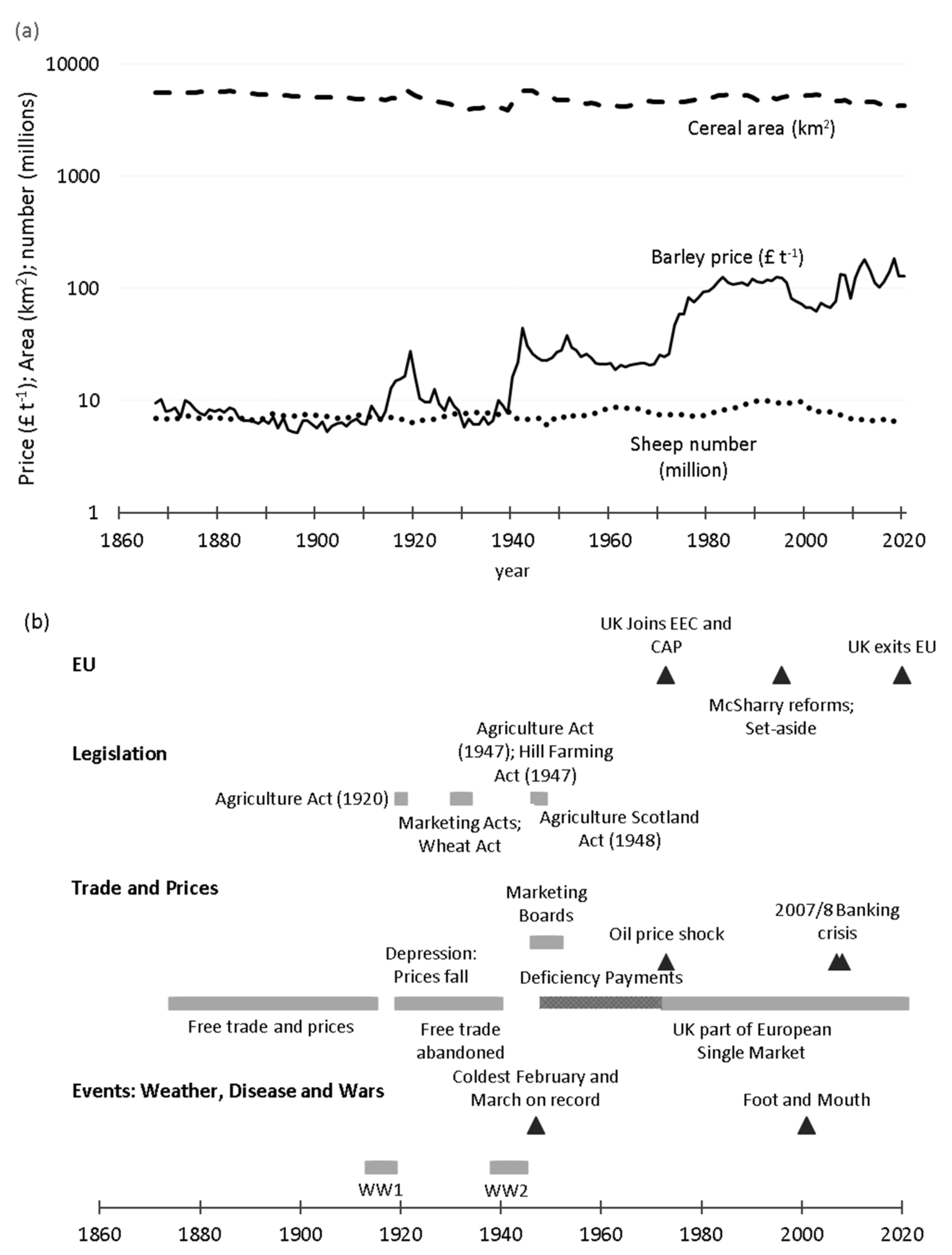
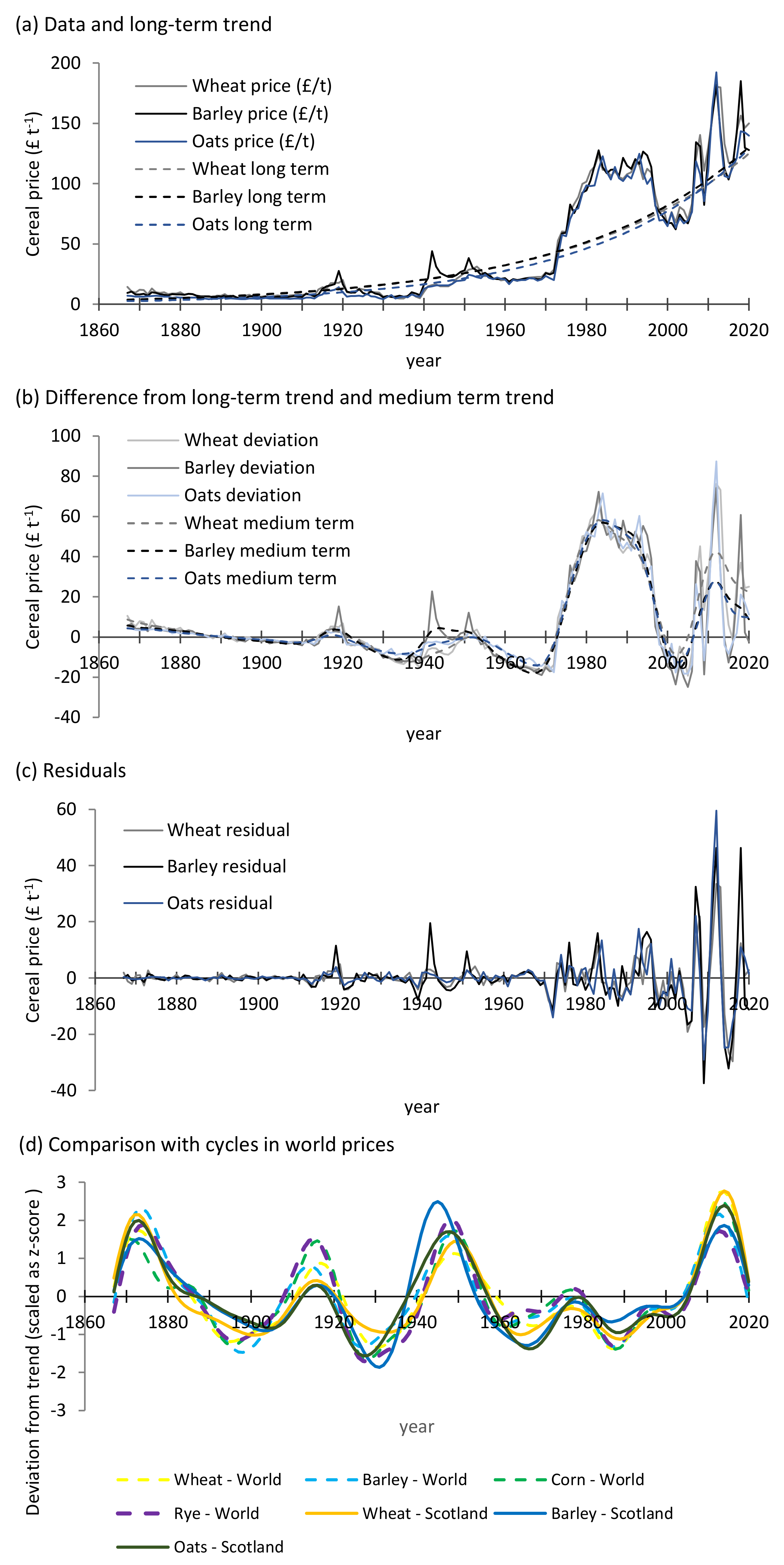
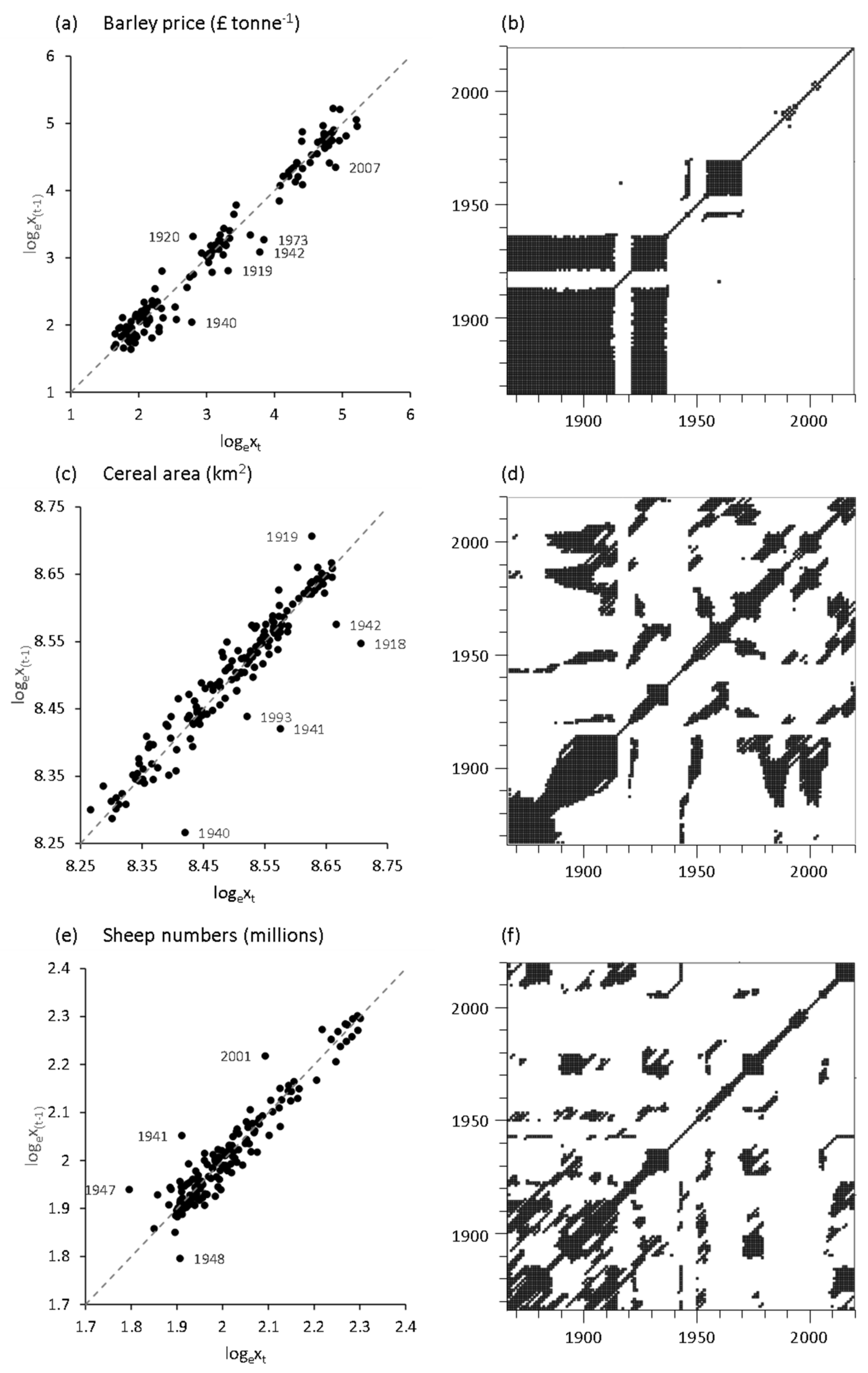
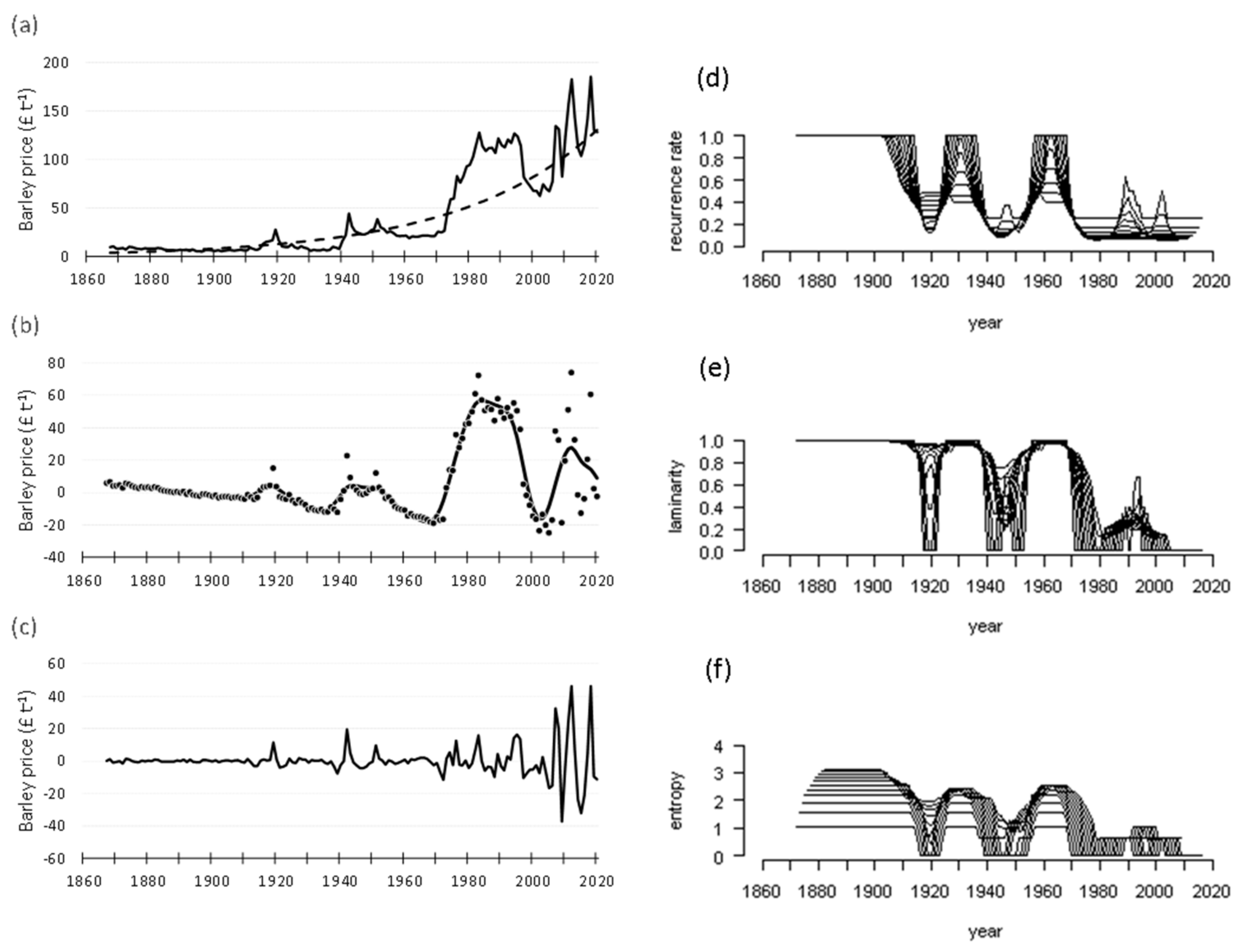
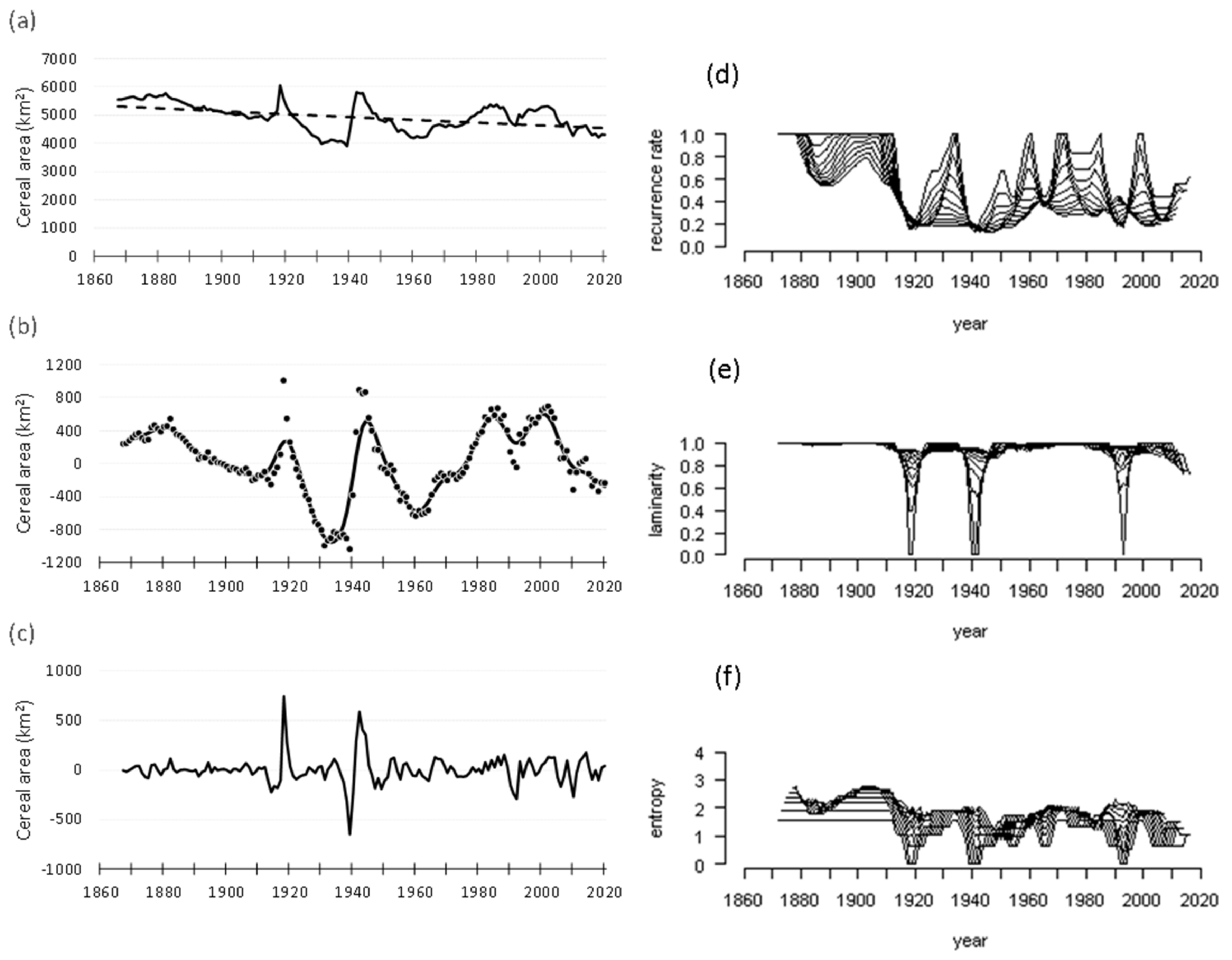
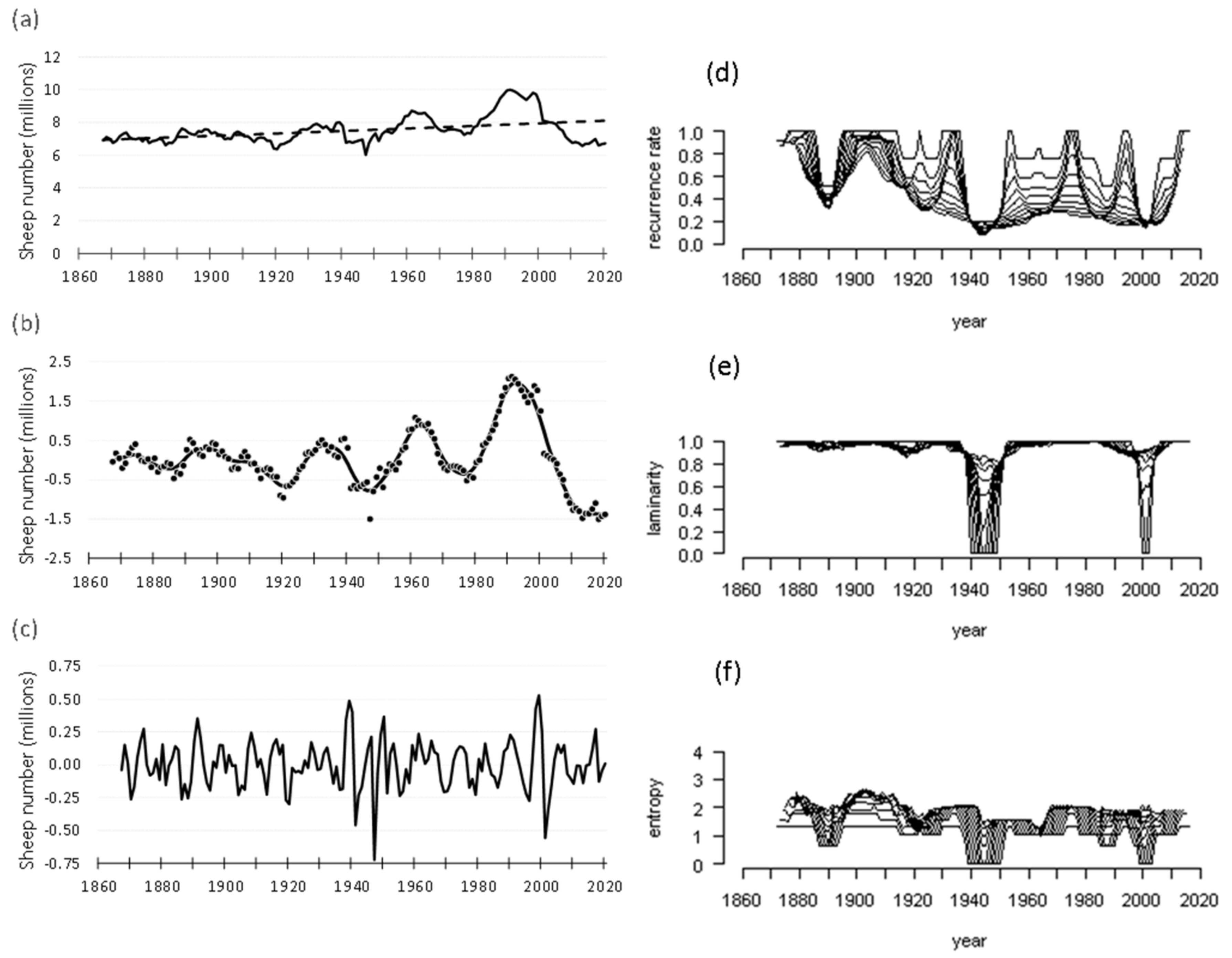
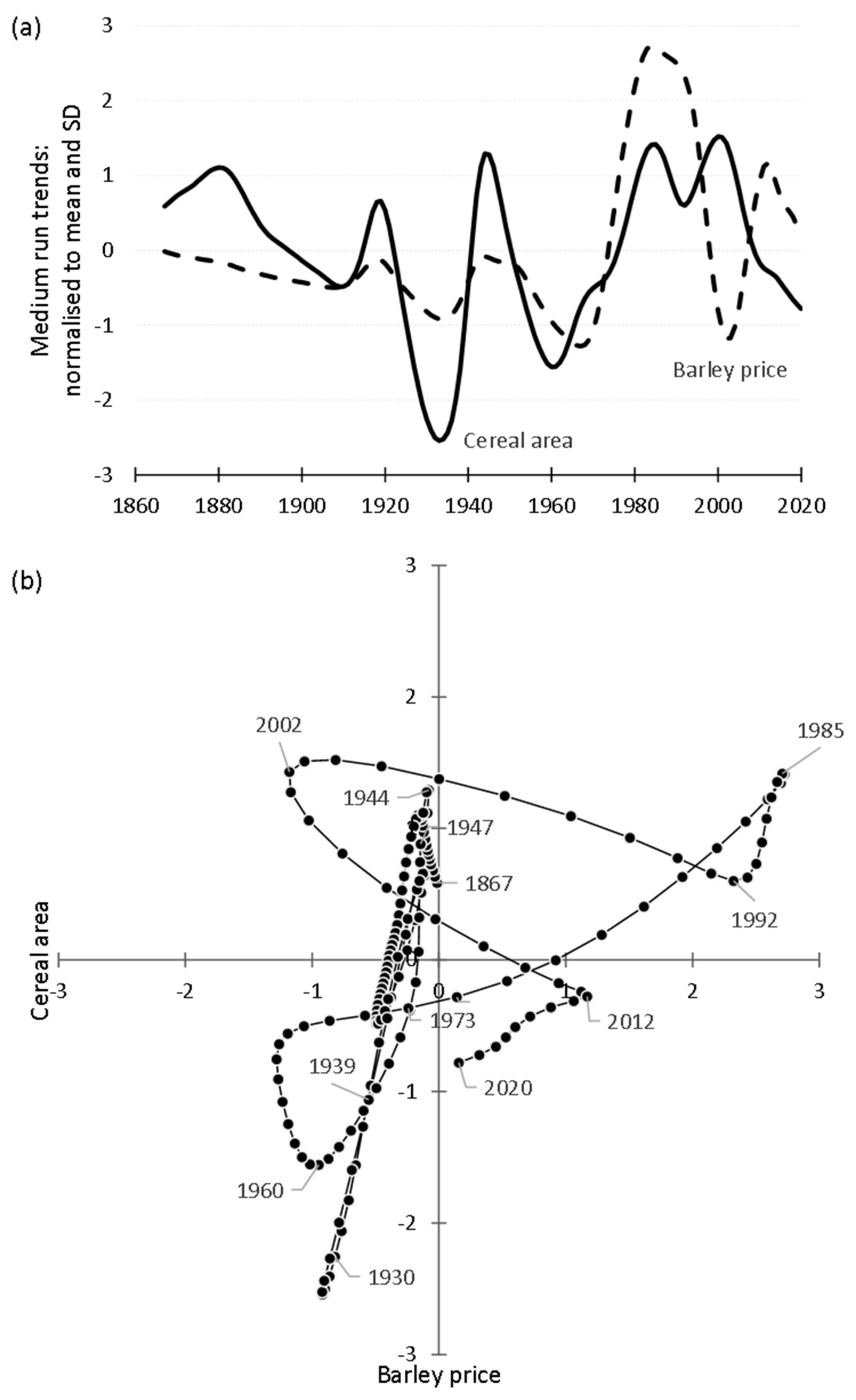
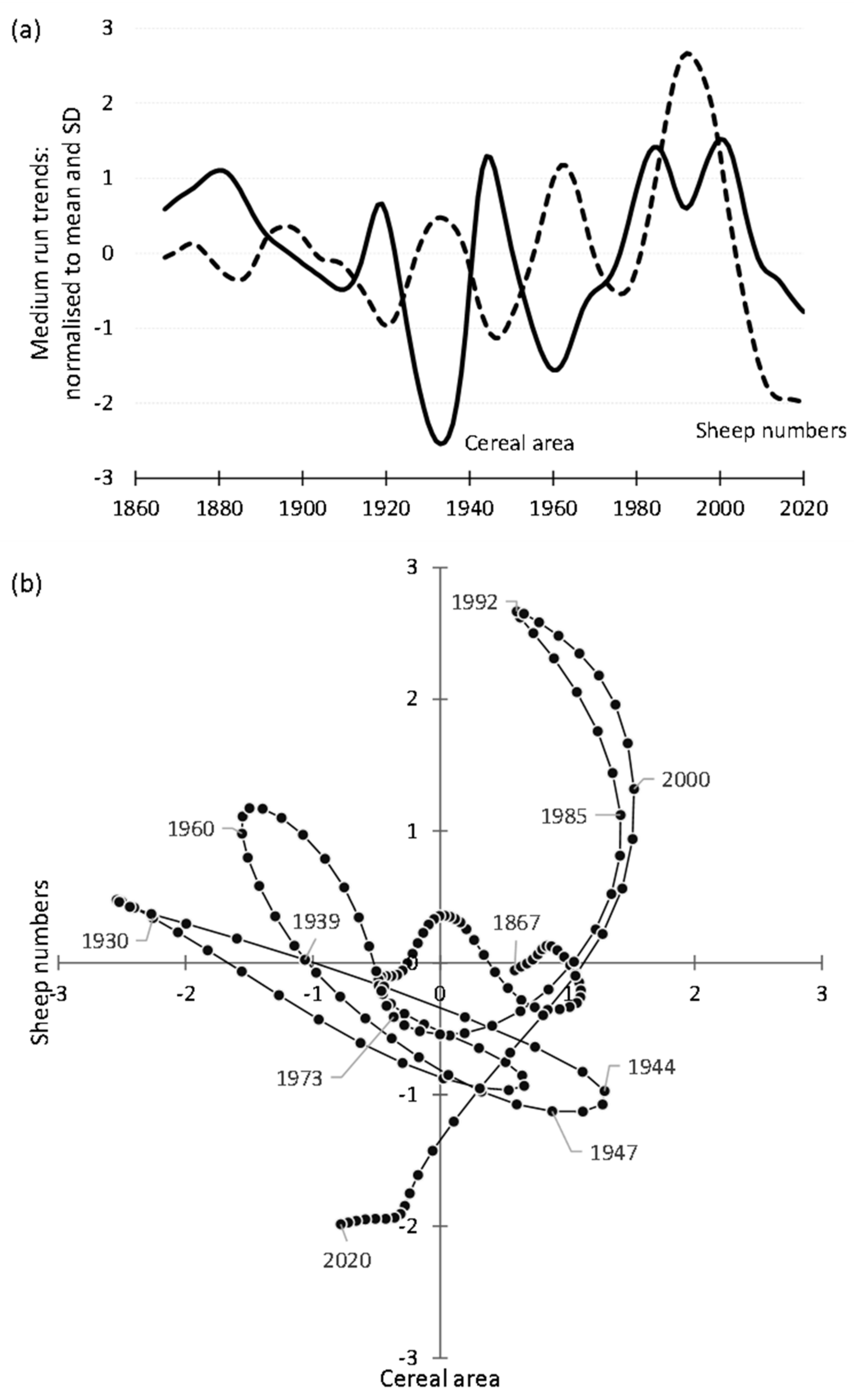
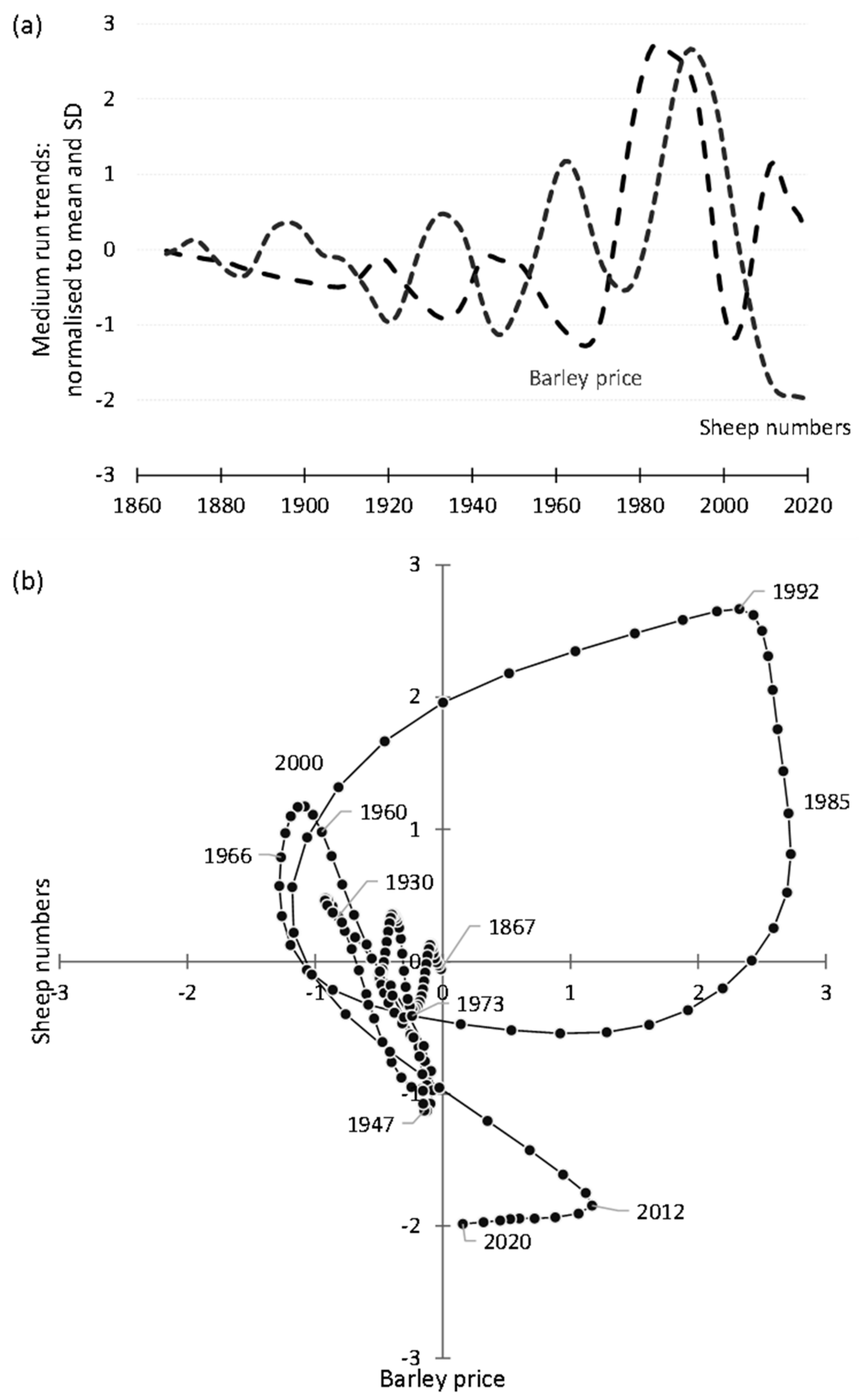
Table 1.
Regression models for prices of cereals (1867–2020).
| Cereal Price (£/Tonne) | Exponential Growth Equation | t-Test for Exponent | F-Test | Variance Explained (R2) |
|---|---|---|---|---|
| Wheat price | t = 23.90 p < 0.0001 | F = 571.1 df: 1 and 152 p < 0.0001 | 78.9% | |
| Barley price | t = 26.41 p < 0.0001 | F = 687.2 df: 1 and 152 p < 0.0001 | 82.1% | |
| Oats price | t = 29.28 p < 0.0001 | F = 687.2 df: 1 and 152 p < 0.0001 | 84.9% | |
for x 1..154 (1867..2020) | ||||
Table 2.
Correlation coefficients (upper right quadrant) and r2 (lower left quadrant) between medium-term cycles for 1867–1946, 1947–1972, and 1973–2020.
Table 2.
Correlation coefficients (upper right quadrant) and r2 (lower left quadrant) between medium-term cycles for 1867–1946, 1947–1972, and 1973–2020.
| Barley Price | Cereal Area | Sheep Numbers | |
|---|---|---|---|
| 1867–1946 | |||
| Barley price | 0.967 | −0.528 | |
| Cereal area | 93.6% | −0.503 | |
| Sheep numbers | 27.9% | 25.3% | |
| 1947–1972 | |||
| Barley price | 0.653 | −0.857 | |
| Cereal area | 42.6% | −0.905 | |
| Sheep numbers | 73.4% | 82.0% | |
| 1973–2020 | |||
| Barley price | 0.157 n.s. | 0.358 n.s. | |
| Cereal area | 2.5% | 0.764 | |
| Sheep numbers | 12.8% | 58.4% | |
Publisher’s Note: MDPI stays neutral with regard to jurisdictional claims in published maps and institutional affiliations. |
© 2021 by the authors. Licensee MDPI, Basel, Switzerland. This article is an open access article distributed under the terms and conditions of the Creative Commons Attribution (CC BY) license (https://creativecommons.org/licenses/by/4.0/).
Share and Cite
MDPI and ACS Style
Aspinall, R.; Staiano, M.; Pearson, D. Emergent Properties of Land Systems: Nonlinear Dynamics of Scottish Farming Systems from 1867 to 2020. Land 2021, 10, 1172. https://doi.org/10.3390/land10111172
AMA Style
Aspinall R, Staiano M, Pearson D. Emergent Properties of Land Systems: Nonlinear Dynamics of Scottish Farming Systems from 1867 to 2020. Land. 2021; 10(11):1172. https://doi.org/10.3390/land10111172
Chicago/Turabian StyleAspinall, Richard, Michele Staiano, and Diane Pearson. 2021. "Emergent Properties of Land Systems: Nonlinear Dynamics of Scottish Farming Systems from 1867 to 2020" Land 10, no. 11: 1172. https://doi.org/10.3390/land10111172
Note that from the first issue of 2016, this journal uses article numbers instead of page numbers. See further details here.