Explaining Non-Take-up of Water Subsidy

Abstract

We use two separate quasi-natural experiments to explore the relative importance of information and administrative costs in explaining non-take-up of water subsidy. The first “experiment” shows that the take-up rate of a household with lower administrative costs is not significantly different from otherwise identical households. In contrast, using the same program, the second “experiment” reveals that the take-up rate of a household that is more likely to be informed is substantially higher compared to otherwise identical households. These findings support the idea that information plays a major role in explaining non-take-up of water subsidy.

1. Introduction

In a recent survey on the explanations for low take-up of social benefits Currie [1] has concluded that “after many years of research, we still have relatively little insight into precisely what types of cost matter most.” Low take-up rate occurs across countries as well as social programs. Estimates of the extent of take-up of social benefits, including our case, range between 40 and 80 percent [2].

A standard cost-benefits model suggests that eligible households would apply if the expected benefits are higher than the cost (See [3] and more recently [4]). The straightforward implication is that for a given level of benefits a negative relation exists between the costs and take-up rates of social benefits.

There are three main types of costs that affect take-up rates: (i) information costs—the costs of collecting and processing information necessary to take-up social benefits. (ii) administrative costs—the costs of applying for social benefits such as water subsidy that may include direct expenses related to the application process and the value of forgone time associated with filling up forms application and waiting in queues. (iii) stigma costs—psychological costs that people may incur during the process of colleting social benefits as they may be perceived by others as either being unable to support themselves or dishonest as they pretend to be deserving and receive unjustifiable welfare benefits [5].

The current state of this literature reflects two main difficulties in estimating the relative significance of information costs, administrative costs and stigma. First, the different costs of participation in a social program such as Food Stamps are likely to interact. For example, a higher degree of complexity may simultaneously raise both information and administrative costs. The challenge to isolate the effect of each factor is even higher because of the interaction between the potential effect of stigma on take-up in means-tested programs and information/administrative costs.

Therefore, it is difficult to estimate the marginal effect of various factors based on a general purpose survey as it has been done in many studies [6]. The attempt to exploit variation in household characteristics in order to study the relative importance of the three competing explanations for low take-up rate is questionable. Most household characteristics tend to influence more than one factor at the same time and these estimates are exposed to a severe problem of selection bias.

For example, education is commonly used to explain variation in take-up rates, but it simultaneously affects stigma, information and administrative costs. High education levels tend to lower the cost of information but at the same time might be associated with higher social and psychological costs (stigma). In addition, higher education may increase (foregone wage) or decrease the cost of administration (a lower cost of filling out forms).

Second, using a general purpose survey to explore the effect of different causes is likely to encounter difficulties in the definition of take-up. The information yielded in such surveys is often much broader than the detailed data needed to define eligibility for social benefits, especially for mean-tested programs. Thus, take-up rates are likely to be measured with large errors that affect the precision of the estimates.

The water subsidy program in Israel which has run for more than 30 years provides an ideal environment to estimate the relative importance of the three competing explanations for non-take-up. This program has an attractive design: an extremely low degree of complexity and supposedly no stigma costs and yet the take-up rate is around 70%, which is well within the range found in most welfare programs [2].

The water pricing structure in Israel consists of three increasing block tariffs (IBT). In 2008, the lowest price applied to the first 96 m³ on a yearly basis (first block), additional consumption up to 84 m³ is subject to an intermediate price (second block), and any extra consumption is charged at the highest price (third block).

In addition, households larger than four persons, that are more likely to be at low income level, are entitled to an additional 36 m³ per person per year at a low rate. Thus, the pricing structure has both quantity-based targeting and characteristic-based targeting to provide low income households with an affordable rate for the most basic commodity—water. This paper focuses on the latter feature of water subsidy. The two reliable sources we have on the reported and actual household size allow us to provide estimates based on a precise definition of take-up.

The monetary value of that additional quantity of water per person could be up to 8 percent of annual water expenditures but for most households it is around 5–6 percent in each year for approximately the next 20 years (see below). The water subsidy here should not be associated with stigma because it is not means-tested [7]. Every household, regardless of its income or wealth is entitled to this water subsidy. Moreover, the receipt of water subsidy is not likely to be seen by others. It is often thought that a recipient may incur stigma if the receipt of social benefits can be observed by others [8].

In this program, the water subsidy is non-automatic and a household must complete a very simple form to take-up that subsidy. The form should include only the names and ID numbers of all household members, and may be sent by regular mail (cost of a stamp) or via fax (cost of a phone call). Thus, the marginal effect of information and administrative costs could be better isolated in light of the low level of complexity and negligible or no stigma costs.

The detailed dataset we have, allows us to employ two separate quasi-experiments in order to estimate the relative importance of information and administrative costs. This identification strategy is less exposed to the selection bias problems encountered by using a general purpose survey. We assume no stigma cost given the features of the program. To study the effect of administrative costs, the take-up rates of two groups of households following a household expansion are compared. Administrative cost appears to be an important factor in several studies [8,9,10,11,12,13,14,15]. For comprehensive surveys see [1,2,6]. The first group, which serves as a control group, consists of four-member households that had expanded to six members in two consecutive years. This group had to apply twice to receive the maximum water subsidy. The second group is composed of households of four members that expand to six members by giving birth to twins, and therefore had to apply only once to receive the maximum water subsidy.

Thus, while the two groups are entitled to the same level of water subsidy (for a given price) they incur different direct administrative costs. The treated group (twins) faces lower administrative costs and as a result has a greater (net) monetary incentive to collect the water subsidy. This gap in administrative costs is exploited to test whether households that expand to six members by giving birth to twins react differently in terms of taking-up their water subsidy as compared to a control group.

To explore the relative importance of information costs we follow the take-up patterns of two groups of households following a household expansion by one member [16,17,18,19]. The first group consists of five-member households that had expanded to six members, and for which the information on water subsidy was already relevant prior to the current household expansion. This group of households had the monetary incentive to search for information regarding the program before the current household expansion, and is used here as our treated group. The second group, which serves as a control group, is composed of households of four members that expand to five members. The information for the second group was immaterial in the past and became relevant with the household’s current expansion.

This information gap is used to test whether households who were potentially exposed to information for a longer period of time react differently in terms of taking-up their water subsidy as compared to a control group of households when a household of either type expands by one member. Both groups of households face the same (direct) administrative cost. In addition, all households are entitled to the same monetary value of water subsidy as a result of the current household expansion.

In the next section we describe the water subsidy that is associated with the water pricing in Israel. Section 3 shows the data and presents the definition of take-up. Section 4 provides the estimates of administrative costs on take-up and Section 5 presents the quantitative role of information costs in determining take-up rates of water subsidy. Section 6 offers the conclusions.

2. Water Subsidy in Israel

The water subsidy that is the focus of this paper is provided to all households in Israel as a reduced price for one of the most basic commodities—water. This pricing arrangement accounts for both efficiency and equity considerations: the highest marginal price reflects efficiency, where it roughly covers the marginal cost, whereas the low price of the first block aims to allow relatively easy access to water consumption for the poor [20,21].

The pricing structure of water in Israel consists of three increasing block tariffs (IBT) [22]. In 2008, the price in the first block, applying to the first 96 m³, was 5.46 Israeli Shekels per m³ or $1.2/m³ including a sewage surcharge. The price in the second block, for additional consumption up to 84 m³, was $1.6/m³. The charge for all extra consumption was $2.2/m³.

This pricing structure has an additional feature. Households larger than four persons are entitled to an additional 36 m³ per person per year at a low rate [23]. Poor families tend to be large, and this characteristic maintains that consideration in the IBT pricing structure (see [24]). In [24] Table 3 shows that 8% of households with 4 members are below poverty line while 17.8% of households with 6 members are below the poverty line. This particular feature has been an integral part of IBT structure for more than 30 years, and is universal but non-automatic.

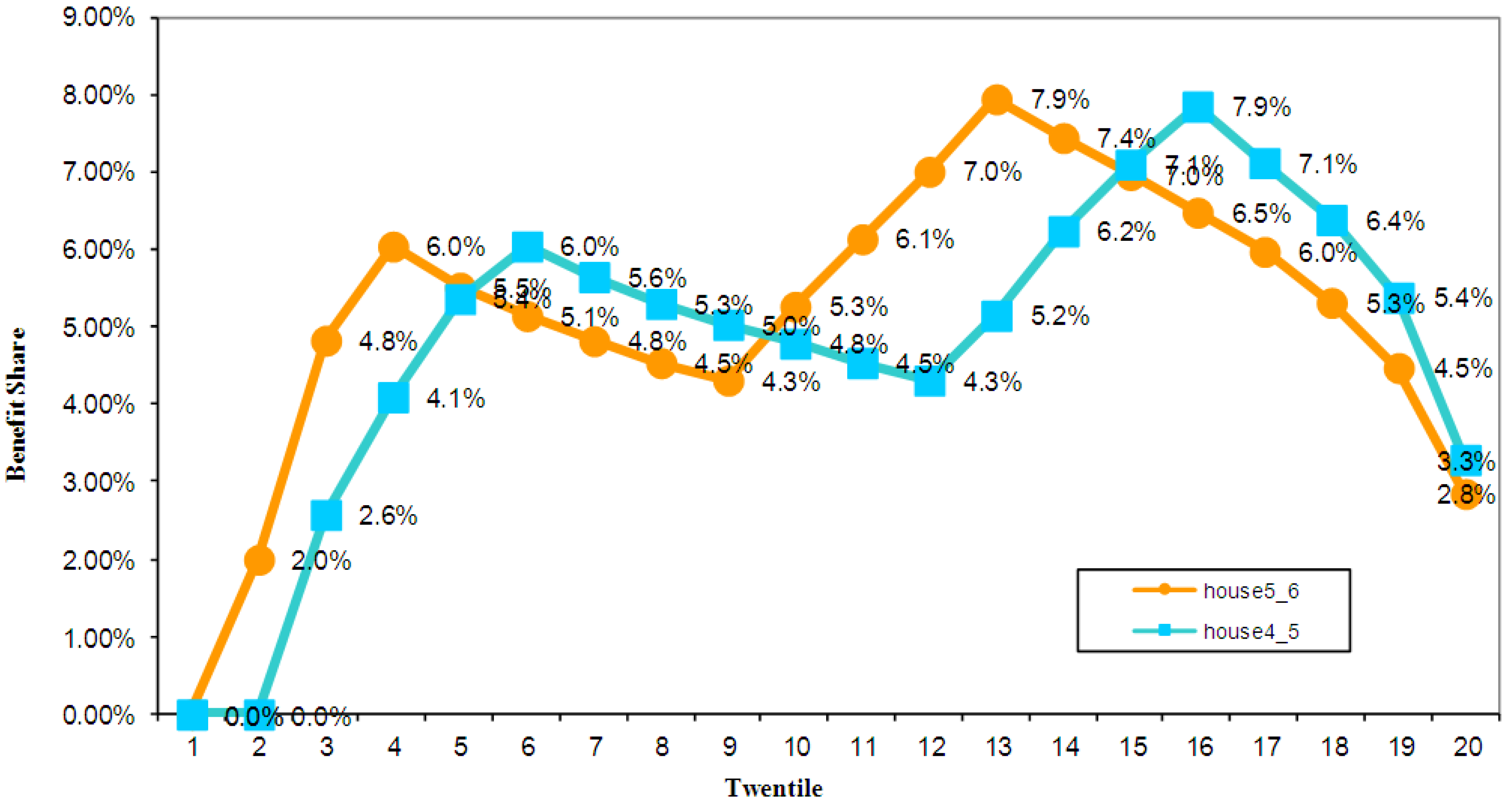
Water subsidy is defined in this paper as the difference between the current (virtual) water bill in the case of reporting on household size and virtual (current) water bill in the case of non-reporting. In Figure 1 water subsidy has been computed using that definition. As can be seen in Figure 1, the water subsidy depends non-linearly on the level of water consumption due to IBT pricing structure. For example, the maximum yearly water subsidy for an additional household member equals the difference between the highest and lowest price multiplied by the supplementary quantity, which equals to $36 a year or 8 percent of annual water expenditures in each year for about the next 20 years (for most households, this is around 5–6 percent). The maximum present value of water subsidy per person is approximately $500. The water subsidy could even be zero if water consumption is low enough (below 60 m³). It is zero because that household faces the same lowest price regardless of the additional quantity of water given after household expansion. Figure 1 shows that it is true for a very small share of households (less than 5%).

To obtain the supplementary quantity of water at a low price, a household must fill out a very simple form: half a page requesting only the names and ID numbers of all household members, and the attached birth certificate of the newborn household member. A family automatically receives a birth certificate immediately after a baby is born (there is no additional cost for a replacement certificate). The form may be sent by regular mail or via fax. Thus, the subsidy in water consumption is associated with extremely low direct administrative costs: cost of a stamp or a phone call. Nevertheless, households may incur additional indirect administrative costs.

Figure 1. The Level of Benefits by Twentiles (as a share of annual water expenditure before household expansion).

Figure 1. The Level of Benefits by Twentiles (as a share of annual water expenditure before household expansion).

A household must report to the water utility provider every time a new member joins the household in order to receive the supplementary quantity of water at a low price. This water subsidy may continue for years until a member leaves the household. According to the law, the water subsidy starts on the reporting date onward (no retroactive incidence). The water subsidy takes effect immediately after reporting (i.e., the next billing period). There is no uncertainty regarding the outcome of the application process and in practice no rejections occur.

Reporting the number of household members does not require sharing information regarding the household’s economic condition such as income, wealth or working status with the water utility officials—information that may be associated with psychological or social costs as in the case of income maintenance or unemployment benefits. The additional quantity of water at a low rate is given to every household regardless of income. Thus, the universality nature of water subsidy reduces the role of stigma in determining take-up rates.

3. Data

The dataset comes from three main sources: the (only) water utility provider in Jerusalem (“Hagihon”); the Municipality of Jerusalem; and the Israel Ministry of the Interior. One important feature of this dataset is that for the same household we have information on household size from two different sources: household size as reported to the water utility provider and household size as documented in the Ministry of the Interior at the end of each year.

Merging the data from these two sources allows us to identify those households that are entitled to the water subsidy but do not collect it, which enables us to define eligibility and take-up in a relatively precise way.

A household is defined as taking up water subsidy if the number of individuals reported to the water utility provider is the same as that which appears in the official files in the Ministry of the Interior. The assumption here is that the size of a household in the official files is also the actual size. These data files are used by the Israeli government for many purposes, such as determining child allowance eligibility, elections, and drafting the relevant population into the military.

The definition of take-up that is used may include households that have ex-post zero water subsidy due to a low level of water consumption in the current year and seemingly have no incentive to report. However, more than 95 percent of the households in the datasets used here are either at the intermediate or highest marginal price level [25].

4. The Role of Administrative Costs

This section presents the first quasi-natural experiment to identify the quantitative effect of program complexity on take-up. We use the same program and the same empirical strategy of quasi-natural experiment to study also the role of information in determining take-up. This second quasi-natural experiment would be presented in Section 5. Using two separate “experiments” to study take-up rates of the same program enable us to provide the relative importance of the two main explanations for non-take-up.

4.1. Constructing the Datasets

The original dataset covers all households in Jerusalem for the years 1999–2003 but our main working population consists of households of four members that had expanded to six during that period according to the official files (i.e., the Ministry of Interior) [26].

Three different datasets were constructed that differ only in time distance between the date of household expansion (entitlement date) and when the reporting status is examined (date of take-up status). All three datasets are composed of households of four members that had expanded to six members by giving birth to twins or by one child (singleton) each year for two consecutive years during the years 2000–2003 [27].

The first dataset detects the reporting status (take-up) after one year [28]. For example, the reporting status is detected at the end of 2001 for a household that was composed of four members in 1999, had expanded by one member in 2000, and gave birth to an additional child in 2001. As can be seen from Table 1 (first row), our dataset contains 89 such households while the total number of households that had expanded to six members and their reporting status is detected after one year is 358 (Table 1).

In the second dataset the reporting status is examined two years after the household had expanded to six members and remains six thereafter. This second dataset consists of 215 households which is smaller than that of the first dataset. This is because households that gave birth to twins in 2003 or had expanded by one child (singleton) in each year for the two consecutive years 2002–2003 have to be excluded as two years after the expansion is out of our period range. In addition, households that had expanded to seven or more must be excluded (they are entitled to a higher level of water subsidy). Likewise, in the third dataset, which consists of 72 households, the reporting status is checked three years after the household had expanded to six members. For example, this dataset includes households that were composed of four members in 1999, gave birth to twins in 2000 (or 2001) or had expanded by one child (singleton) in each year for the two consecutive years 2000–2001. Again, households that had expanded to seven (or more) were excluded from the analysis.

Table 1. The working datasets—number of households by type and reporting status.

Type of household expansion	Year(s) of household expansion	Years since household expansion (at which we detect the status of reporting)
		One year	Two years	Three years
Two singletons twins	2000–2001 2000	89 25	78 22	39 15
Two singletons twins	2001–2002 2001	89 28	72 22	-- 18
Two singletons twins	2002–2003 2002	87 26	-- 21	-- --
Two singletons twins	-- 2003	-- 14	-- --	-- --
Total number of households		358	215	72

Table 1. The working datasets—number of households by type and reporting status.

Type of household expansion	Year(s) of household expansion	Years since household expansion (at which we detect the status of reporting)
		One year	Two years	Three years
Two singletons twins	2000–2001 2000	89 25	78 22	39 15
Two singletons twins	2001–2002 2001	89 28	72 22	-- 18
Two singletons twins	2002–2003 2002	87 26	-- 21	-- --
Two singletons twins	-- 2003	-- 14	-- --	-- --
Total number of households		358	215	72

Table 2. Descriptive statistics.

Explanatory variables	One year b	Two years c	Three years d
Apartment size (square meter) a	69.0	68.9	72.1
Annual water consumption (cubic meter) a	175.7	178.6	186.8
Orthodox Jews (share) a	0.55	0.53	0.42
Arabs (share) a	0.06	0.07	0.10
Households at the lowest price (share) a	0.08	0.08	0.07
Take-up: overall	0.19	0.59	0.71
Take-up: twins	0.28	0.68	0.79
Take-up: singleton	0.16	0.55	0.64
Number of observations	358	215	72

^a As documented before a household expansion; ^b The first dataset contains three different panels for singleton’s households (1999–2001, 2000–2002 and 2001–2003) and four panels for twins’ households (1999–2000, 2000–2001, 2001–2002 and 2002–2003). The reporting status is checked one year (at the end) after the household had expanded to six; ^c The second dataset consists of two different panels for singleton’s households (1999–2002 and 2000–2003) and three panels for twins’ households (1999–2001, 2000–2002, and 2001–2003). The reporting status is checked two years (at the end) after the household had expanded to six; ^d The third dataset consists of one panel for singleton’s households (1999–2003) and two panels for twins’ households (1999–2002, and 2000–2003). The reporting status is checked three years (at the end) after the household had expanded to six.

Table 2. Descriptive statistics.

Explanatory variables	One year b	Two years c	Three years d
Apartment size (square meter) a	69.0	68.9	72.1
Annual water consumption (cubic meter) a	175.7	178.6	186.8
Orthodox Jews (share) a	0.55	0.53	0.42
Arabs (share) a	0.06	0.07	0.10
Households at the lowest price (share) a	0.08	0.08	0.07
Take-up: overall	0.19	0.59	0.71
Take-up: twins	0.28	0.68	0.79
Take-up: singleton	0.16	0.55	0.64
Number of observations	358	215	72

^a As documented before a household expansion; ^b The first dataset contains three different panels for singleton’s households (1999–2001, 2000–2002 and 2001–2003) and four panels for twins’ households (1999–2000, 2000–2001, 2001–2002 and 2002–2003). The reporting status is checked one year (at the end) after the household had expanded to six; ^c The second dataset consists of two different panels for singleton’s households (1999–2002 and 2000–2003) and three panels for twins’ households (1999–2001, 2000–2002, and 2001–2003). The reporting status is checked two years (at the end) after the household had expanded to six; ^d The third dataset consists of one panel for singleton’s households (1999–2003) and two panels for twins’ households (1999–2002, and 2000–2003). The reporting status is checked three years (at the end) after the household had expanded to six.

Table 2 presents take-up rates using the definition outlined above. Collecting the water subsidy is involved with both low costs and benefits and yet the overall take-up rate among households of four members that become six is around 60 percent two years after the expansion, which is well within the range of take-up rates in social programs in OECD countries [2].

The take-up rate of four-member households that become six by giving birth to twins is higher (68 percent) as compared to the take-up rate among households of four members that become six by one child (singleton) each year for two consecutive years (55 percent). The difference is between 12 to 15 percentage points, depending on the time distance between the date of household expansion and when the reporting status is examined. It takes time to collect the water subsidy associated with reporting, as is evident in Table 2. The take-up rate after two years is more than twice as much as the rate after one year.

4.2. Identification Strategy

A natural prediction of cost-benefit analysis of take-up is that a household will decide to collect the water subsidy as long as benefits are greater than costs, regardless of income level [29]. The administrative costs, that include both direct cost of sending the application form and the time invested in filling up the application and sending it, may be lower or higher than the value of water subsidy. The administrative costs are likely to exceed water subsidy for those households that consume small amount of water and therefore are entitled to low level of water subsidy. These households are not expected to report on household size. In contract, households that are characterized with low earnings ability face lower administrative costs as the value of their time is low and are expected to take-up water subsidy at higher rates.

As in many other social programs, both the level of water subsidy as well as participation costs depends on household characteristics. For example, households that consume a relatively small quantity of water and consequently are entitled to a lower level of subsidy might also face lower indirect costs (forgone earnings) in collecting that water subsidy due to lower earning ability. Note that the direct costs here are fixed for all households. However, it could be associated with higher rather than lower indirect costs for poor households to the extent that colleting and processing information is a decreasing function of education level. This association between the level of subsidy and participation costs introduce an empirical challenge.

To cope with the above empirical challenge two groups of households were constructed. The first group—the treated group—is a four-member household that expanded by two members (twins) at the beginning of the respective period. The second group—the control group—is a four-member household that expanded by two members (singletons), but in two consecutive years.

In general, the twins-event may not be exogenous and might be correlated with household characteristics. For example, households with high income may have better access to infertility treatment and therefore may be characterized by a higher probability of having twins. This might be true for the first or even the second birth but is unlikely to affect households who have already two children as in the “experiment” used here.

These two groups are identical in the following sense: they both entitled to an additional 72 m³ of water at a low rate. For a given price, the monetary value of water subsidy is the same for both groups but they face different level of direct administrative costs.

A household may declare on one, two or even more additional members on the same form. This feature implies that a household belongs to the treated group has to file an application form only once in order to collect the water subsidy, while a household from the control group must file twice.

A household from the control group might decide to wait a year or more and file only after the second household expansion in anticipation of that expansion. However, waiting is costly given the way the water subsidy program was designed. A household who decides to file only after the second expansion would lose a year (or more) of water subsidy due to the no retroactive incidence of that subsidy.

Thus, the direct administrative costs of the treated group are smaller compared to the control group, either directly or indirectly, through the cost of waiting. Note that the direct administrative costs are relatively low in this program. Obviously, there are other indirect costs that may also play a role such as the value of time.

The assignment of a household to one of the two groups is not completely random. Households of five-members who decide to have an additional child are a selective group, and that potentially introduces selection bias which might be caused by two different factors. First, parents who decide to have a child at parity n + 1 might not be comparable to parents who decide to have a child at parity n and unintentionally had twins. Second, within the sample of parents who give birth at parity n + 1, those who have an additional child one year after the previous child are a selective group that might be characterized by low socio-economic background and high religiosity levels.

Table 3. Comparison of treated and control group.

Time distance between examining reporting status and expansion	Household type: treated and control groups	No. of observations	Average Apartment Size (square meter) a	Average Share of Orthodox Jews a	Average Share of Arabs a	Average Annual water consumption (cubic meter) a
After one year	4 turn 6	93	74.09	0.39	0.03	203.1
	4 turn 5 & 6	265	67.27	0.61	0.06	166.1
t statistic b			2.44	−3.74	−1.15	4.26
After two years	4 turn 6	65	74.73	0.43	0.05	198.6
	4 turn 5 & 6	150	66.25	0.58	0.07	169.9
t statistic b			2.65	−2.02	−0.74	2.57
After three years	4 turn 6	33	76.55	0.36	0.06	196.7
	4 turn 5 & 6	39	68.12	0.46	0.13	178.5
t statistic b			1.52	−0.83	−0.96	0.97

^a Before household expansion; ^b t statistics for mean’s difference between the control and treated groups. The numbers in bolds reflect statistical significance.

Table 3. Comparison of treated and control group.

Time distance between examining reporting status and expansion	Household type: treated and control groups	No. of observations	Average Apartment Size (square meter) a	Average Share of Orthodox Jews a	Average Share of Arabs a	Average Annual water consumption (cubic meter) a
After one year	4 turn 6	93	74.09	0.39	0.03	203.1
	4 turn 5 & 6	265	67.27	0.61	0.06	166.1
t statistic b			2.44	−3.74	−1.15	4.26
After two years	4 turn 6	65	74.73	0.43	0.05	198.6
	4 turn 5 & 6	150	66.25	0.58	0.07	169.9
t statistic b			2.65	−2.02	−0.74	2.57
After three years	4 turn 6	33	76.55	0.36	0.06	196.7
	4 turn 5 & 6	39	68.12	0.46	0.13	178.5
t statistic b			1.52	−0.83	−0.96	0.97

^a Before household expansion; ^b t statistics for mean’s difference between the control and treated groups. The numbers in bolds reflect statistical significance.

Indeed, Table 3, which presents household characteristics for both groups before the expansion, shows that the treated group has a larger apartment size, and constitutes a lower share of Orthodox Jews and Arabs. However, the difference is not always significant and in particular the difference between the two groups is insignificant when limiting the comparison to those who had not expanded for three years after expanding to six. In the estimated equations, ethnic background and water consumption level will be controlled for to account for these differences between the treated and control groups.

Our main goal is to test whether the treated group reacts differently in terms of take-up of water subsidy as compared to the control group, following a household expansion by two members.

4.3. Estimation Models

Two alternative models are estimated: the first model does not control for any household characteristics while the other model addresses a potential effect of the differences in household characteristics and a year effect.

First model:

$$\left(\text{1}\right){\text{y}}_{\text{i}}=\text{a}+{\text{bD}}_{\text{i}}+{\text{ε}}_{\text{i}},$$

and second model:

$$\left(\text{2}\right){\text{y}}_{\text{i}}=\text{α}+\text{β}{\mathbf{\text{x}}}_{\text{i}}+\text{γ}{\text{D}}_{\text{i}}+{\text{δ}}_{\text{j}}{\text{t}}_{\text{j}}+{\text{ε}}_{\text{i}},$$

where, y_i is a dummy variable that is equal to one for a household that had reported the same household size as appears in the official files, and otherwise zero. x_i denotes a vector of household characteristics before household expansion and D_i represents the dummy variable for the treatment effect. D_i is a binary variable that equals 1 for a treated household and zero for a control household. We also control for a year effect, t_j where there are two separate year effects in the case of three panels, one year effect in the case of two panels and no year effect in the case of a three years panel.

The vector x includes two main household characteristics that may affect take up rate of water subsidy: ethnic groups (the share of Orthodox Jews and Arabs) and the virtual marginal price of water faced by a household which represents the level of water subsidy.

In Jerusalem there are two large distinct ethnic groups with significantly higher levels of poverty: Orthodox Jews and Arabs. An Orthodox Jewish household is defined as such if it is located in an Orthodox neighborhood as designated in the Jerusalem master plan. The same is true for a household defined as Arab.

The actual level of water subsidy may differ depending on the actual level of water consumption that determines the marginal price paid by a household. The virtual marginal price is used to estimate the effect of the level of water subsidy on take-up rates [30]. A marginal virtual price is defined as the marginal price that would have been faced by a household given its actual water consumption in the event of no reporting on household size.

4.4. Results

Three versions are used to estimate the effect of administrative costs, as captured by our treatment dummy variable, according to the time gap between the year of household expansion to six members and the date the reporting is checked. In the first version, take up status is defined based on the reporting status of a household a year after a household had expanded to six. The second and third versions are based on reporting status two and three years after the household expansion, respectively.

Logit regressions are employed with and without control variables for household characteristics. We present the marginal effects which are easier to interpret: the units are percentage points of take-up rates. Table 4 reports the coefficients and z statistics for the two estimated models.

In the first column of Table 4, take up (the dependent variable) is defined according to the status of reporting at the end of the expansion year. Using a regression without any control variable, the coefficient of the treated group is both positive and significant (around 12 percentage points as implied by the marginal effects). The magnitude of the treatment effect is similar when take up is defined according to the reporting status at the end of the second or third year from the household expansion to six; however it is not statistically significant.

Table 4. Effect of administrative costs on take-up rates: Logit estimation. (Dependent variable: reporting status in year t).

Explanatory variables	After one year		After two years		After three years
Intercept	−1.64	−1.53	0.19	0.68	0.58	0.80
	(−9.85)	(−2.50)	(1.14)	(0.93)	(1.74)	(0.69)
Twins (4 turn 6)	0.69	0.62	0.55	0.20	0.73	0.22
	(2.44)	(1.81)	(1.77)	(0.51)	(1.35)	(0.30)
2001		−0.15		−1.19		−0.92
		(−0.27)		(−1.78)		(−0.92)
2002		−0.49		−0.52		-
		(−0.88)		(−0.77)
2003		−0.03		-		-
		(−0.05)
Arabs		0.27		−1.34		−1.13
		(0.44)		(−1.89)		(−1.14)
Orthodox Jews		0.15		0.56		0.97
		(0.51)		(1.78)		(1.40)
Virtual lowest price		−1.12		−0.59		−0.48
		(−1.47)		(−1.10)		(−0.46)
Virtual highest price		0.18		0.68		1.53
		(0.64)		(2.09)		(2.22)
Pseudo R2	0.0164	0.0346	0.0111	0.0958	0.0218	0.1815
Number of observations	358	358	215	215	72	72

z statistics are in parentheses.

Table 4. Effect of administrative costs on take-up rates: Logit estimation. (Dependent variable: reporting status in year t).

Explanatory variables	After one year		After two years		After three years
Intercept	−1.64	−1.53	0.19	0.68	0.58	0.80
	(−9.85)	(−2.50)	(1.14)	(0.93)	(1.74)	(0.69)
Twins (4 turn 6)	0.69	0.62	0.55	0.20	0.73	0.22
	(2.44)	(1.81)	(1.77)	(0.51)	(1.35)	(0.30)
2001		−0.15		−1.19		−0.92
		(−0.27)		(−1.78)		(−0.92)
2002		−0.49		−0.52		-
		(−0.88)		(−0.77)
2003		−0.03		-		-
		(−0.05)
Arabs		0.27		−1.34		−1.13
		(0.44)		(−1.89)		(−1.14)
Orthodox Jews		0.15		0.56		0.97
		(0.51)		(1.78)		(1.40)
Virtual lowest price		−1.12		−0.59		−0.48
		(−1.47)		(−1.10)		(−0.46)
Virtual highest price		0.18		0.68		1.53
		(0.64)		(2.09)		(2.22)
Pseudo R2	0.0164	0.0346	0.0111	0.0958	0.0218	0.1815
Number of observations	358	358	215	215	72	72

z statistics are in parentheses.

As noted earlier, the treated and control groups are not entirely identical in their characteristics. The second estimated model appearing in Table 4 shows that the effect of treatment is slightly lower, after controlling for ethnic groups and price indicators and a year effect. However, the significance of that coefficient does not survive the inclusion of the control variables. The estimated coefficient implies that the take up rate of the treated group is around 4 percentage point higher, but this is not even borderline significant.

The sign of all control variables are as expected, but are not always significant. However, the level of water subsidy, which is represented by the virtual price, positively affects take-up rates as implied by the coefficient of the highest virtual price.

A possible concern with the identification strategy employed here is that there might be many variables that differ across families having twins versus a singleton birth which might affect the costs and benefits to participate. For example, the children’s health status and the labor supply choices of parents could differ. To address that concern we compare the take-up rates of two groups: a three-member household that expanded by two members (twins) and a second group that is a four-member household that expanded by one member (singletons). Both groups are entitled to the same level of water subsidy (an additional 36 m³ of water at a reduced price) and face exactly the same direct administrative costs (apply only once).

Table 5 presents the results of that additional quasi-experiment. It is shown that the take-up rates of twins’ households are not significantly different from that of a singleton. This finding suggests that the results of the main “experiment,” which implies no significant effect of administrative costs on take-up, are not driven by factors that are correlated with twins’ households.

Table 5. Effect of administrative costs on take-up rates—robustness test: Logit estimation. (Dependent variable: reporting status in year t).

Explanatory variables	After one year		After two years		After three years
Intercept	−1.38	−1.78	−0.35	−0.51	−0.20	0.02
	(−28.47)	(−15.10)	(−6.35)	(−4.30)	(−2.00)	(0.13)
Twins (3 turn 5)	0.15	0.29	0.35	0.50	0.20	0.04
	(0.61)	(1.13)	(1.18)	(1.64)	(0.41)	(0.07)
00–01		0.10
		(0.82)
01–02		−0.12
		(−0.99)
00–02				−0.02
				(−0.20)
Arabs		−1.06		−1.47		−1.21
		(−3.01)		(−4.05)		(−2.57)
Orthodox Jews		0.84		0.76		0.38
		(8.41)		(6.50)		(1.60)
Virtual price A		−0.63		−0.90		−1.25
		(−2.67)		(−3.17)		(−2.33)
Virtual price C		0.27		−0.01		−0.26
		(2.70)		(−0.10)		(−1.24)
Pseudo R2	0.0001	0.0415	0.0007	0.0481	0.0003	0.0350
Number of observations	2,753	2,753	1,425	1,425	439	439

z statistics are in parentheses.

Table 5. Effect of administrative costs on take-up rates—robustness test: Logit estimation. (Dependent variable: reporting status in year t).

Explanatory variables	After one year		After two years		After three years
Intercept	−1.38	−1.78	−0.35	−0.51	−0.20	0.02
	(−28.47)	(−15.10)	(−6.35)	(−4.30)	(−2.00)	(0.13)
Twins (3 turn 5)	0.15	0.29	0.35	0.50	0.20	0.04
	(0.61)	(1.13)	(1.18)	(1.64)	(0.41)	(0.07)
00–01		0.10
		(0.82)
01–02		−0.12
		(−0.99)
00–02				−0.02
				(−0.20)
Arabs		−1.06		−1.47		−1.21
		(−3.01)		(−4.05)		(−2.57)
Orthodox Jews		0.84		0.76		0.38
		(8.41)		(6.50)		(1.60)
Virtual price A		−0.63		−0.90		−1.25
		(−2.67)		(−3.17)		(−2.33)
Virtual price C		0.27		−0.01		−0.26
		(2.70)		(−0.10)		(−1.24)
Pseudo R2	0.0001	0.0415	0.0007	0.0481	0.0003	0.0350
Number of observations	2,753	2,753	1,425	1,425	439	439

z statistics are in parentheses.

5. The Role of Information Costs

5.1. Constructing the Datasets

To examine the role of information in determining take-up patterns of water subsidy we use the same database that covers all households in Jerusalem for the years 1999–2002 to extract our working datasets. In the following empirical analysis we use only those households of four and five members that had had expanded by one member in the years 2000–2002. Three different datasets are constructed that differ in time distance between the date of household expansion and when we detect the reporting status. The first dataset detects the reporting status (take-up) of households of four and five members that had had expanded by one member in the years 2000–2002 after one year. For example, the reporting status is detected at the end of 2000 for a household that was composed of four or five members in 1999 and had expanded by one member in 2000, a half year after the expansion on average (For the sake of conciseness, we use one year, two years and three years instead of a half year, a year and a half and two years and half, respectively). Table 6 (first row), shows that there were 853 households of four members in 1999 that had expanded by one member in 2000. The first dataset covers 2,220 households of five members that become six and 2,656 four-member households that expanded by one member (Table 6).

Table 6. The working datasets—number of households by reporting status and household type.

Type of household expansion	Year of household expansion	Years since household expansion (at which we detect the status of reporting)
		One year	Two years	Three years
4→5	2000	853	678	421
5→6	2000	759	610	377
4→5	2001	893	699	--
5→6	2001	695	570	--
4→5	2002	910	--	--
5→6	2002	766	--	--
Total 4→5		2,656	1,377	421
Total 5→6		2,220	1,180	377
Total number of households		4,876	2,557	798

Table 6. The working datasets—number of households by reporting status and household type.

Type of household expansion	Year of household expansion	Years since household expansion (at which we detect the status of reporting)
		One year	Two years	Three years
4→5	2000	853	678	421
5→6	2000	759	610	377
4→5	2001	893	699	--
5→6	2001	695	570	--
4→5	2002	910	--	--
5→6	2002	766	--	--
Total 4→5		2,656	1,377	421
Total 5→6		2,220	1,180	377
Total number of households		4,876	2,557	798

In the second dataset we follow the same household for three consecutive years. This covers those households of four or five members in 1999 that had expanded, for example, in 2000 and their reporting status (take-up) is examined at the end of the 2001, a year and a half after the expansion on average. The third dataset is composed of households that had expanded in 2000 and their reporting status (take-up) is detected at the end of 2002, two years and a half after the expansion on average. In both the second and third datasets, those households that were expanded more than once were excluded because those households are entitled to double (or even triple) water subsidy.

Table 7 presents take-up rates using the definition outlined above. The take-up rate among households of five members that become six is around 55 percent three years after the expansion which is well within the range of take-up rates in social programs in OECD countries [2]. The take-up rate of five-member-households (that become six) is higher compared to the take-up rate among households of four members that become five (41 percent). The differences are similar regardless of the time distance we use.

Table 7. Take-up rates for different time distances.

Years since household expansion	Take-up rates
	4 that become 5 (Control Group)	5 that become 6 (all) Treated Group	5 that become 6 and reported on the fifth member	5 that become 6 but did not report on the fifth member
after one year	0.20	0.28	0.36	0.13
1999–2000	0.21	0.31	0.39	0.15
2000–2001	0.22	0.29	0.37	0.15
2001–2002	0.18	0.23	0.33	0.11
after two years	0.41	0.52	0.63	0.32
1999–2001	0.42	0.53	0.64	0.29
2000–2002	0.41	0.51	0.61	0.34
after three years (1999–2002)	0.45	0.55	0.64	0.35

Table 7. Take-up rates for different time distances.

Years since household expansion	Take-up rates
	4 that become 5 (Control Group)	5 that become 6 (all) Treated Group	5 that become 6 and reported on the fifth member	5 that become 6 but did not report on the fifth member
after one year	0.20	0.28	0.36	0.13
1999–2000	0.21	0.31	0.39	0.15
2000–2001	0.22	0.29	0.37	0.15
2001–2002	0.18	0.23	0.33	0.11
after two years	0.41	0.52	0.63	0.32
1999–2001	0.42	0.53	0.64	0.29
2000–2002	0.41	0.51	0.61	0.34
after three years (1999–2002)	0.45	0.55	0.64	0.35

Time distance matters, as is evident in Table 7. The take-up rate after two years is almost twice as much as the rate after one year. Clearly, it takes time to collect the social benefit associated with reporting. The take-up after three years is just slightly higher compared to two years. For example, the take-up rate among households of five members that become six is 28 percent after one year, 52 percent after two years and 55 percent three years after the expansion.

5.2. Identification Strategy

In order to examine the role of information we distinguish between two separate groups of households. These two groups are identical in the following sense: they both expanded by one member at the beginning of the respective period. The first group (previously-entitled households) consists of five members who had expanded to six and for which the information regarding water subsidy is valuable prior to the current household expansion. Those households apparently had the monetary incentive to search for that information.

The second type (newly-entitled households) consists of four members that expanded to five. Those households did not have the incentive to report according to the rules of the program. It should be recalled that the price structure of water is the same for every household up to four members, regardless of household size. Therefore, there is no water subsidy associated with additional members as long as the household is four members or less.

The first type of household had the incentive to search for information regarding the water subsidy associated with reporting before the current household expansion, while for the second type the information was immaterial in the past and became relevant with the current expansion [31]. We use the time difference since a household became first entitled to water subsidy as a proxy for the state of information. Potentially, the previously-entitled households (“treated” group) possess more information than the newly-entitled households (control group) because of the longer time that has been elapsed since these households became first entitled to water subsidy as compared to the control group. The previously-entitled households are hypothesized to have more information due to the longer time they had the monetary incentive to search for that information.

Previously-entitled (“treated”) and newly-entitled (control) households all face the same administrative process for reporting on the current household expansion. Consequently, the direct administrative cost is the same for all households. In addition, both groups are entitled to the same level of water subsidy (for a given price) as a result of the current expansion [32]. A household above four members is entitled to an additional 36m³ of water at a low rate for each additional member regardless of its size.

Thus, we could better isolate the effect of information gap between previously-entitled and newly-entitled households given that both the level of water subsidy and (direct) administrative costs are the same following the current expansion of a household by one member. We follow the take-up rates of both types of households for up to three years after the expansion.

Note, that the previously-entitled group is composed of two household sub-groups: households of five members who expanded to six and had reported in the past on the fifth member and households of five members who expanded to six but had not reported on the fifth member. Those households that had reported on the fifth member apparently were in possession of the information on water subsidy before the current expansion.

Those households are presumably informed but we cannot rule out that this group may be a selection of households that had faced lower administrative cost in the previous household expansion. Likewise, the behavior of households that did not report on the fifth member may be consistent with two conflicting hypotheses: those households were truly uninformed and consequently they had not collected their water subsidy following the previous household expansion or they were fully informed but decided not to report because of cost-benefit considerations.

Thus, using households that had reported on the fifth member as an alternative “treated” group may be exposed to a self-selection problem. This risk of self-selection problem is important to the extent that cost-benefit considerations that dictate the decision to report in the past on the fifth member is correlated with the conditions following the current household expansion. Therefore, we use instead all five-member households who became six as our “treated” group.

Our main goal is to test whether the previously-entitled group reacts differently in terms of take-up of water subsidy as compared to the newly-entitled group, when a household of either type is expanded by one member. We hypothesize that those households which for a longer period of time had the incentive to collect information would tend to have higher take-up rates.

By its construction, the previously-entitled group is larger by one member than the control group, and that may generate differences in household characteristics. Table 8 presents household characteristics for both groups. It shows that the previously-entitled group has a larger apartment size but is smaller in terms of apartment size per capita. It is unclear which group is wealthier; this depends on the assumed economies of scale in housing.

The share of Orthodox Jews is higher (statistically significant) among the previously-entitled group because they tend to have more children. For the other three characteristics: Arab population, below poverty line indicator and price level, the difference is not always significant. In the estimation section we will control for these characteristics.

Table 8. Descriptive statistics—a comparison of previously-entitled and control groups *.

Status date	Household type	Explanatory variables	Apartment Size	The share of households
				Orthodox Jews	Arabs	Below poverty line	At (actual) intermediate or highest price
One year	5 turn 6	Obs	1,668	2,220	2,220	2,220	2,220
		Mean	76.8	0.49	0.08	0.02	0.95
		Std	23.7	0.5	0.27	0.14	0.22
	4 turn 5	Obs	1,894	2,656	2,656	2,656	2,656
		Mean	73.2	0.36	0.06	0.01	0.97
		Std	21.6	0.48	0.23	0.12	0.18
		Means’ Difference	3.56	0.13	0.02	0.01	−0.02
		t statistic	4.65	9.23	2.79	1.27	−3.03
Two Years	5 turn 6	Obs	938	1,180	1,180	1,180	1,180
		Mean	78.1	0.48	0.08	0.02	0.95
		Std	23.7	0.5	0.27	0.13	0.22
	4 turn 5	Obs	1,083	1,377	1,377	1,377	1,377
		Mean	74.6	0.35	0.06	0.014	0.96
		Std	22.7	0.48	0.23	0.12	0.19
		Means’ Difference	3.50	0.12	0.03	0.004	0.01
		t statistic	3.38	6.44	2.52	0.81	1.71
Three Years	5 turn 6	Obs	308	377	377	377	377
		Mean	81.89	0.31	0.11	0.03	0.95
		Std	25.18	0.46	0.32	0.16	0.21
	4 turn 5	Obs	350	421	421	421	421
		Mean	77.14	0.21	0.08	0.02	0.97
		Std	23.84	0.41	0.27	0.15	0.17
		Means’ Difference	4.75	0.1	0.04	0.01	−0.01
		t statistic	2.48	3.26	1.7	0.25	−1.43

* The data in this table refer to the year before household expansion.

Table 8. Descriptive statistics—a comparison of previously-entitled and control groups *.

Status date	Household type	Explanatory variables	Apartment Size	The share of households
				Orthodox Jews	Arabs	Below poverty line	At (actual) intermediate or highest price
One year	5 turn 6	Obs	1,668	2,220	2,220	2,220	2,220
		Mean	76.8	0.49	0.08	0.02	0.95
		Std	23.7	0.5	0.27	0.14	0.22
	4 turn 5	Obs	1,894	2,656	2,656	2,656	2,656
		Mean	73.2	0.36	0.06	0.01	0.97
		Std	21.6	0.48	0.23	0.12	0.18
		Means’ Difference	3.56	0.13	0.02	0.01	−0.02
		t statistic	4.65	9.23	2.79	1.27	−3.03
Two Years	5 turn 6	Obs	938	1,180	1,180	1,180	1,180
		Mean	78.1	0.48	0.08	0.02	0.95
		Std	23.7	0.5	0.27	0.13	0.22
	4 turn 5	Obs	1,083	1,377	1,377	1,377	1,377
		Mean	74.6	0.35	0.06	0.014	0.96
		Std	22.7	0.48	0.23	0.12	0.19
		Means’ Difference	3.50	0.12	0.03	0.004	0.01
		t statistic	3.38	6.44	2.52	0.81	1.71
Three Years	5 turn 6	Obs	308	377	377	377	377
		Mean	81.89	0.31	0.11	0.03	0.95
		Std	25.18	0.46	0.32	0.16	0.21
	4 turn 5	Obs	350	421	421	421	421
		Mean	77.14	0.21	0.08	0.02	0.97
		Std	23.84	0.41	0.27	0.15	0.17
		Means’ Difference	4.75	0.1	0.04	0.01	−0.01
		t statistic	2.48	3.26	1.7	0.25	−1.43

* The data in this table refer to the year before household expansion.

5.3. The Estimated Models

We estimate two alternative models: the first model does not control for any household characteristics while the other model addresses a potential effect of the differences in household characteristics and a year effect.

First model:

$$\left(\text{1}\right){\text{y}}_{\text{i}}=\text{a}+{\text{bD}}_{\text{i}}+{\text{ε}}_{\text{i}},$$

and second model:

$$\left(\text{2}\right){\text{y}}_{\text{i}}=\text{α}+\text{β}{\mathbf{\text{x}}}_{\text{i}}+\text{γ}{\text{D}}_{\text{i}}+{\text{δ}}_{\text{j}}{\text{t}}_{\text{j}}+{\text{ε}}_{\text{i}},$$

where, y_i is a dummy variable that is equal to one for a household that had reported, and otherwise zero. x_i denotes a vector of household characteristics in the respective period and D_i represents the dummy variable for the “treatment effect”. This variable represents the longer time since the information on water subsidy became material to a household. D_i is a binary variable that equals 1 for a previously-entitled household and zero for a newly-entitled (control) household. We also control for a year effect, t_j where there are two separate year effects in the case of three panels, one year effect in the case of two panels and no year effect in the case of three years panel.ε_i

The vector x includes an array of household characteristics that may affect reporting behavior. There are three types of variables: wealth indicators (apartment size, garden size and poverty indicator), social network indicators (Orthodox Jews and Arabs), language barrier (Arabs) and the virtual marginal price of water faced by a household which represents the level of water subsidy.

The net effect of wealth on take-up is uncertain. According to Moffitt [3], take-up rates should be falling as wealth rises due to lower marginal utility. In contrast, take-up rates might not be affected directly by wealth level as long as the cost of participation enters welfare function directly. In addition, wealth may affect take-up rates indirectly (through the connection between education and wealth) because we do not control for education in our regressions. A wealthier household may incur lower costs in collecting and processing information given the positive relations between wealth and education.

According to the recent literature, we hypothesize that a household that belongs to a social network is more likely to be informed and as a result would have higher probability of reporting [33,34,35,36]. In Jerusalem there are two large distinct ethnic groups that may be classified as social networks: Orthodox Jews and Arabs. Each one of these two groups maintains close personal relations internally and has little social connection with the rest of the population. In fact, the Arab population has almost no social connection with the Jewish population.

In addition, an Arab household may face a language barrier. Although the criteria for an additional quantity of water at a low rate are outlined both in Hebrew and Arabic on the back page of every water bill, the application form is available in Hebrew only. Part of the Arab population in East Jerusalem who affiliate themselves with the Palestinian Authority tend to minimize the frequency of contact with Israeli official authorities. Therefore, they may be less exposed to information regarding their entitlement to water subsidy. The Arab population may face lower information cost due to the social network, but at the same time incurs higher information cost due to language barrier. Thus, the net effect must be examined empirically.

As noted before, both the previously-entitled and control groups are entitled to the same additional quantity of water at a low rate following the current expansion by one member. Yet, the actual level of water subsidy may still differ depending on the actual level of water consumption that determines the marginal price paid by a household.

We use the virtual marginal price as a proxy to estimate the effect of the level of water subsidy on take-up rates [37]. A marginal virtual price is defined as the marginal price that would have been faced by a household given its actual water consumption in the event of no reporting on household size.

In general, households that reported on the current expansion face a lower (actual) marginal price as compared to households that did not report. This may affect their actual water consumption to the extent that price elasticity of water demand is negative. The virtual price might be higher for a reporting household and as a result the coefficient might be biased downward. The estimated price elasticity of water demand is relatively low which subdues that bias [24].

5.4. Results

We run Logit regressions, with and without control variables for household characteristics. To estimate the role of information as captured by our dummy variable we use three different datasets, according to the time gap between the year of household expansion and the date the reporting on that expansion is checked. In the first dataset the dependent variable is defined based on the reporting status of a household a year after the expansion. The second and third datasets are based on reporting status two and three years after the household expansion, respectively.

Table 9 reports the coefficients and z statistics for the two estimated models. In a regression without any control variable, the effect of “treatment” is positive and around 7 percentage points (as implied by the marginal effects) even when the reporting status is detected at the end of the expansion year. The magnitude of the “treatment effect” is higher when the reporting status is checked at the end of the second or third year from the household expansion. The estimated effect ranges between 9 to 11 percentage points. Those households for which the information was relevant for a longer period of time indeed have higher take-up rate.

We saw earlier that the previously-entitled and control groups are not completely identical in their characteristics. The second estimated model appearing in Table 9 shows that the coefficient of a previously-entitled household is only slightly lower, even after controlling for various explanatory variables and a year effect. The magnitude of that effect is closer to the first estimated model when reporting status is examined at the end of the second or third year from the household expansion.

Given the nature of the dataset, we control for a year effect in the second estimated model. In the one-year dataset (which is composed of three panels of two years) we found that the 2001–2002 dummy is negative and significant while the other dummy is insignificant. The year effect is not significant in the two-year dataset and by construction there is no year effect in the three-year dataset.

As discussed above, the Arab household dummy variable reflects two conflicting forces in terms of information costs. The negative sign of this coefficient and its magnitude is consistent with the hypothesis that language barrier is much more influential than is the social network. . This coefficient is twice as large when reporting status is checked at the end of the second or third year from household expansion as compared to the end of the household expansion year.

The Orthodox Jewish dummy variable represents a lower information cost due to better social network. As expected, the coefficient is positive but it is statistically significant in two of the three cases.

As expected, the level of water subsidy positively affects take-up rates as implied by the virtual price coefficient. A higher virtual price implies higher water subsidy that induce a household to collect information and report on household size. In general, the coefficient of the intermediate (virtual) price is significantly positive compared to the lowest price, and it is lower than the coefficient of the highest (virtual) price, although this is not always the case. This result is in line with one of the most robust findings in the literature on the reasons for low take-up rates.

In general, all wealth indicators (apartment size by quintiles, garden size and poverty indicator [38]) are insignificant. It can be also in line with the notion that take-up rates are influenced by wealth level due to lower marginal utility [3] but it is canceled out by the effect of a lower information cost associated with higher level wealth, to the extent that wealth and education are correlated.

The effect of a previously-entitled household is even larger where we exclude the two ethnic groups from the datasets (not reported in the tables). The take-up rate of households of five who had expanded to six is 13 percentage points higher when reporting status is checked at the end of the second or third year since household expansion. This estimated effect is not sensitive to the inclusion of control variables.

Table 9. Effect of information costs on take-up rates: Logit estimation. (Dependent variable: reporting status in year t).

Explanatory variables	After One Year		After Two Years		After Three Years
Intercept	−1.38	−2.10	−0.35	−1.45	−0.20	−1.38
	(−28.47)	(−10.03)	(−6.35)	(−6.01)	(−2.00)	(−2.96)
5 turn 6 (All)	0.41	0.29	0.43	0.37	0.40	0.41
	(6.10)	(4.00)	(5.33)	(4.33)	(2.83)	(2.70)
00–01		−0.03
		(−0.37)
01–02		−0.30
		(−3.47)
00–02				−0.11
				(−1.37)
Arabs		−1.35		−1.62		−1.15
		(−5.35)		(−6.58)		(−3.75)
Orthodox Jews		0.62		0.68		0.31
		(8.29)		(7.62)		(1.75)
Virtual Price B		0.65		0.90		1.15
		(3.47)		(4.12)		(2.57)
Virtual Price C		0.91		1.00		1.04
		(4.86)		(4.64)		(2.37)
Apartment Size: Second Quintile		−0.15		0.03		0.10
		(−1.19)		(0.21)		(0.40)
Apartment Size: Third Quintile		0.06		0.17		0.15
		(0.50)		(1.14)		(0.56)
Apartment Size: Fourth Quintile		0.01		0.10		0.31
		(0.07)		(0.66)		(1.18)
Apartment Size: Top Quintile		−0.08		0.04		0.43
		(−0.62)		(0.24)		(1.58)
Apartment Size Unknown		−0.50		−0.15		−0.39
		(−4.25)		(−1.02)		(−1.46)
Poverty Indicator		0.01		−0.21		0.01
		(0.02)		(−0.68)		(0.02)
Garden Owners		0.23		0.15		0.24
		(1.38)		(0.76)		(0.77)
Garden Size		0.00		0.00		0.00
		(1.25)		(1.96)		(0.73)
Pseudo R2	0.0070	0.0537	0.0081	0.0671	0.0073	0.0639
Observations	4,876	4,876	2,557	2,557	798	798

z statistics are in parentheses. * The bottom quintile is omitted.

Table 9. Effect of information costs on take-up rates: Logit estimation. (Dependent variable: reporting status in year t).

Explanatory variables	After One Year		After Two Years		After Three Years
Intercept	−1.38	−2.10	−0.35	−1.45	−0.20	−1.38
	(−28.47)	(−10.03)	(−6.35)	(−6.01)	(−2.00)	(−2.96)
5 turn 6 (All)	0.41	0.29	0.43	0.37	0.40	0.41
	(6.10)	(4.00)	(5.33)	(4.33)	(2.83)	(2.70)
00–01		−0.03
		(−0.37)
01–02		−0.30
		(−3.47)
00–02				−0.11
				(−1.37)
Arabs		−1.35		−1.62		−1.15
		(−5.35)		(−6.58)		(−3.75)
Orthodox Jews		0.62		0.68		0.31
		(8.29)		(7.62)		(1.75)
Virtual Price B		0.65		0.90		1.15
		(3.47)		(4.12)		(2.57)
Virtual Price C		0.91		1.00		1.04
		(4.86)		(4.64)		(2.37)
Apartment Size: Second Quintile		−0.15		0.03		0.10
		(−1.19)		(0.21)		(0.40)
Apartment Size: Third Quintile		0.06		0.17		0.15
		(0.50)		(1.14)		(0.56)
Apartment Size: Fourth Quintile		0.01		0.10		0.31
		(0.07)		(0.66)		(1.18)
Apartment Size: Top Quintile		−0.08		0.04		0.43
		(−0.62)		(0.24)		(1.58)
Apartment Size Unknown		−0.50		−0.15		−0.39
		(−4.25)		(−1.02)		(−1.46)
Poverty Indicator		0.01		−0.21		0.01
		(0.02)		(−0.68)		(0.02)
Garden Owners		0.23		0.15		0.24
		(1.38)		(0.76)		(0.77)
Garden Size		0.00		0.00		0.00
		(1.25)		(1.96)		(0.73)
Pseudo R2	0.0070	0.0537	0.0081	0.0671	0.0073	0.0639
Observations	4,876	4,876	2,557	2,557	798	798

z statistics are in parentheses. * The bottom quintile is omitted.

The coefficients estimated in both models imply a quantitatively large effect. The estimated take-up rate of the previously-entitled group is around 25 percent higher as compared to the control group. This supports the idea that information plays a major role in shaping take-up rates.

6. Conclusions

It is shown that the take-up rate of water subsidy by treated households (twins) which face lower administrative costs is only slightly higher as compared to a control group of households (singleton) that is entitled to same level of water subsidy, and this effect is insignificant. This finding implies that administrative costs do not play a role in a water subsidy program characterized by low benefits and low administrative costs.

In contrast, using the same program, we show that the take-up rate of a household that is more likely to be informed is substantially higher compared to otherwise identical households. The estimated information effect in terms of take-up rates is in the range of 8 and 13 percentage points. This result is robust for different time distances and the inclusion of various household characteristics. In addition, we found that variables that are directly associated with information costs such as social network indicators (Orthodox Jews and Arabs) and language barrier (Arabs) have significant influence on take-up rates.

This paper addresses two challenges faced in the literature on take-up of social benefits. First, the two reliable sources on eligibility and take-up allow us to estimate the relative importance of information and administrative costs based on a precise definition of take-up. Second, the low degree of complexity and negligible (or no) role of stigma of the Israeli water subsidy program investigated here reduce significantly the risk of biased estimates due to the relatively low interaction between various costs of participation. Using a quasi-natural experiment strategy that is less exposed to selection bias problem further helps to isolate the marginal impact of each factor in determining take-up patterns of water subsidy.

While the identification strategy employed here provides a relatively clean estimate of the partial effect of administrative and information costs, this might come with a cost in terms of the generality of the results. The water subsidy program use here to explore the determinants of take up have both very low benefits and costs, and the results might be seem limited to low stakes participation decisions. However, despite these features, the take up rate in this program is around 70 percent in the general population (and 60 percent for households covered in this study), which is well within the range of take-up rates found in social programs in OECD countries [39].

The welfare and policy implications low take-up as a result of lack of information are different from low take-up due to choice of people who are aware of their rights and nevertheless choose not to claim their entitled benefits. Low take-up rate due to information barriers should be a cause of deeper concern for policy makers because it undermines profoundly the policy goals. A natural policy implication of our findings is that the lowering of information barriers is likely to have a significant effect on take-up of social benefits, especially for certain population groups.