
Prediction of Earth Dam Seepage Using a Transient Thermal Finite Element Model

Abstract
:1. Introduction
2. Materials and Methods
2.1. Analytical Method
2.2. Finite Element Method
3. Results
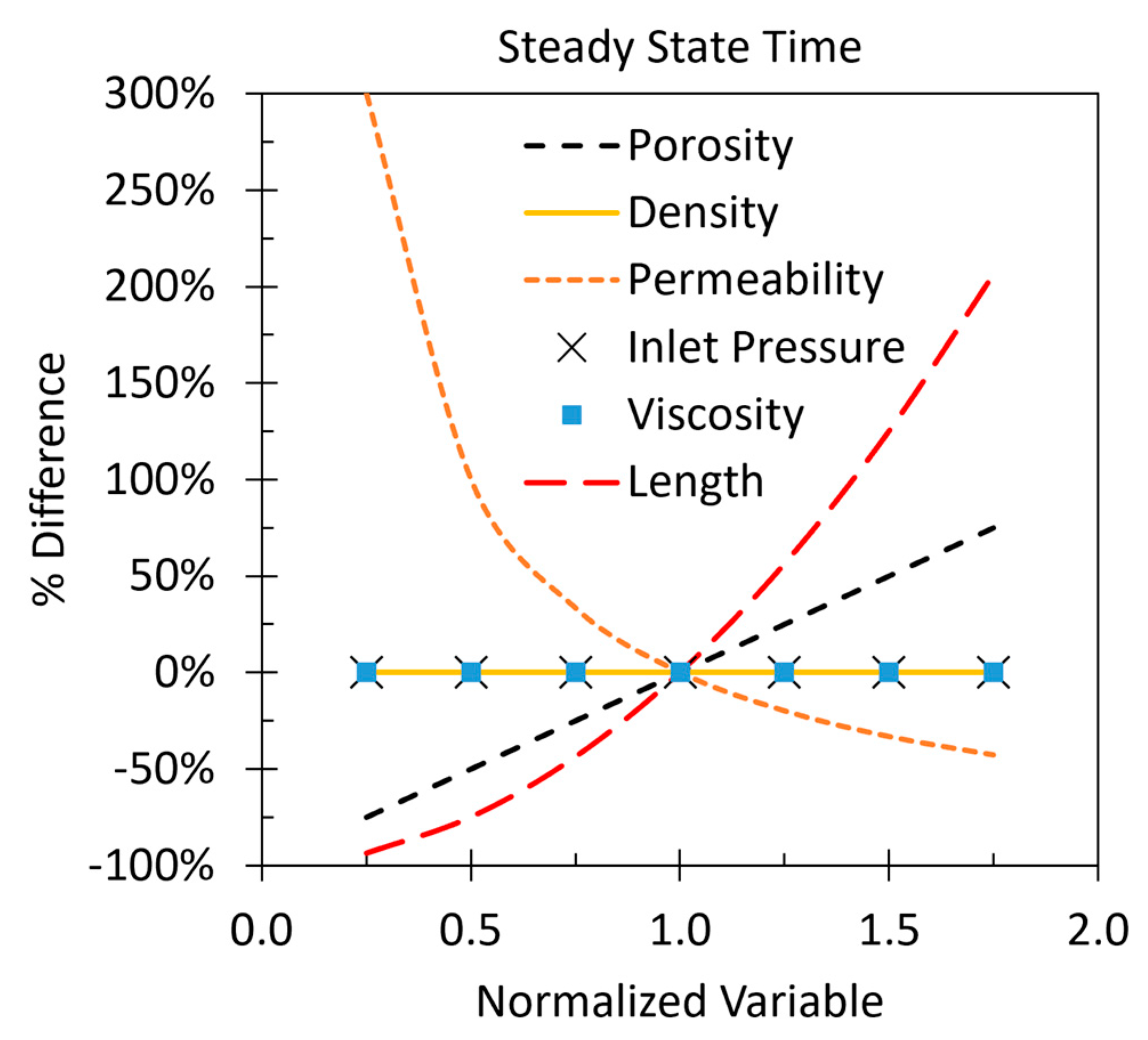
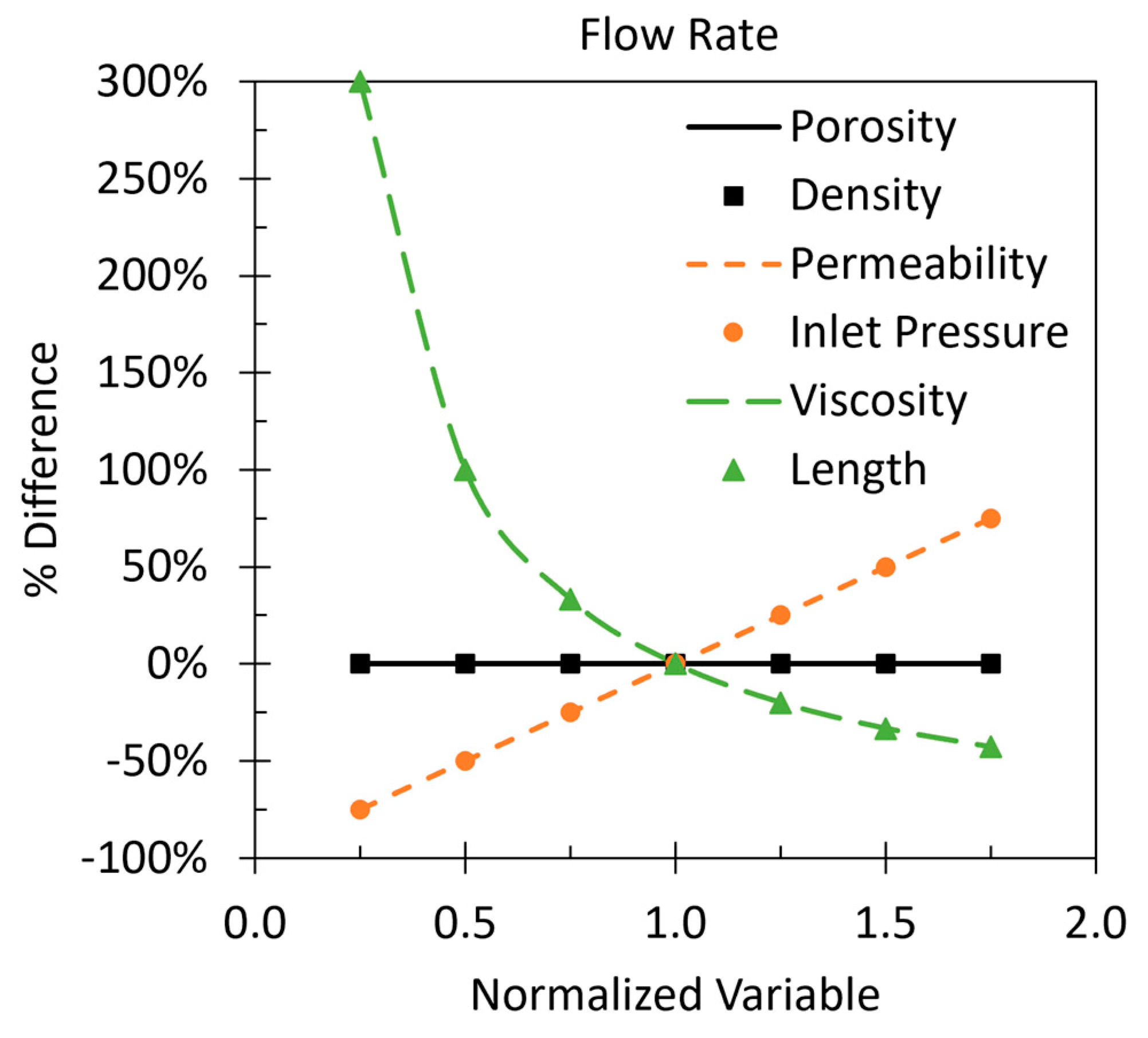
4. Discussion
5. Conclusions
Author Contributions
Funding
Data Availability Statement
Acknowledgments
Conflicts of Interest
References
- FEMA P-911; Assessing Dams and Impoundments: A Beginner’s Guide. USDA US Forest Service: Washington, DC, USA, 2017.
- Association of State Dam Safety Officials (ASDSO). Dam Failure Incident Driver. 2022. Available online: https://damsafety.org/dam-failures (accessed on 7 September 2022).
- Fadaei-Kermani, E.; Shojaee, S.; Memarzadeh, R.; Barani, G.A. Numerical simulation of seepage problem in porous media. Appl. Water Sci. 2019, 9, 79. [Google Scholar] [CrossRef] [Green Version]
- McBride, M.S.; Pfannkuch, H.O. The distribution of seepage within lakebeds. J. Res. US Geol. Surv. 1975, 3, 505–512. [Google Scholar]
- Aniskin, N.A.; Antonov, A.S. Using Mathematical Models to Study the Seepage Conditions at the Bases of Tall Dams. Power Technol. Eng. 2017, 50, 580–584. [Google Scholar] [CrossRef]
- Alekseevich, A.N.; Sergeevich, A.A. Numerical Modelling of Tailings Dam Thermal-Seepage Regime Considering Phase Transitions. Model. Simul. Eng. 2017, 2017, 7245413. [Google Scholar] [CrossRef] [Green Version]
- Dardanelli, G.; Pipitone, C. Hydraulic Models and Finite Elements for Monitoring of an Earth Dam, by Using GNSS Techniques. Period. Polytech. Civ. Eng. 2016, 61, 421–433. [Google Scholar] [CrossRef] [Green Version]
- Zhou, W.; Li, S.; Zhou, Z.; Chang, X. InSAR Observation and Numerical Modeling of the Earth-Dam Displacement of Shuibuya Dam (China). Remote. Sens. 2016, 8, 877. [Google Scholar] [CrossRef] [Green Version]
- Gordan, B.; Adnan, A.; Aida, M.A.K. Soil Saturated Simulation in Embankment during Strong Earthquake by Effect of Elasticity Modulus. Model. Simul. Eng. 2014, 2014, 1–7. [Google Scholar] [CrossRef] [Green Version]
- Szostak-Chrzanowski, A.; Massiéra, M. Relation between monitoring and design aspects of large earth dams. In Proceedings of the 3rd IAG Symposium on Geodesy for Geotechnical and Structural Engineering and 12th FIG Symposium on Deformation Measurements, Baden, Austria, 22–24 May 2006. [Google Scholar]
- Schueler, T.; Holland, H.K. The compaction of urban soils. Watershed Prot. Tech. 2000, 3, 661–665. [Google Scholar]
- Caldwell, L. USDA Watershed Programs Facts and Figures: A Reservoir of Watershed Program Information; U.S. Department of Agriculture Natural Resources Conservation Service (NRCS), Conservation Engineering Division: Washington, DC, USA, 2020.


| Darcy Flow | Heat Equation | ||||
|---|---|---|---|---|---|
| Variable | Value | Variable | Value | ||
| 6.89 × 10⁵ | 6.89 × 10⁵ | ||||
| 0.00 | 0.00 | ||||
| 0.00 | 0.00 | ||||
| 1.00 | 1.00 | ||||
| 1.72 × 10³ | 1.72 × 10³ | ||||
| 1.43 × 10⁻¹⁵ | 1.43 × 10⁻¹² | ||||
| 1.00 × 10⁻³ | () | 4.00 × 10⁻¹² | |||
| 35.7% | () | 2.07 × 10⁻⁴ | |||
| Min. Flow | Max. Flow | Avg. Flow | Theoretical Darcy Flow | |
|---|---|---|---|---|
| (W/m2) | (W/m2) | (W/m2) | (m/s) | |
| 1 year | 0.00 × 100 | 5.15 × 10⁻⁵ | ||
| 10 years | 0.00 × 100 | 1.61 × 10⁻⁵ | 9.85 × 10⁻⁷ | |
| 100 years | 0.00 × 100 | 5.09 × 10⁻⁶ | ||
| Approx. time | 2.96 × 10⁻⁷ | 2.96 × 10⁻⁷ | 9.93 × 10⁻⁷ | |
| 1000 years | 4.32 × 10⁻⁷ | 1.57 × 10⁻⁶ | 9.90 × 10⁻⁷ | |
| 10,000 years | 9.86 × 10⁻⁷ | 9.86 × 10⁻⁷ | 9.86 × 10⁻⁷ |
| Variable | Min. | Base | Max | |
|---|---|---|---|---|
| 1.72 × 10⁵ | 6.89 × 10⁵ | 1.21 × 10⁶ | ||
| 0.25 | 1.00 | 1.75 | ||
| 4.31 × 10² | 1.72 × 10³ | 3.02 × 10³ | ||
| 3.58 × 10⁻¹⁶ | 1.43 × 10⁻¹⁵ | 2.50 × 10⁻¹⁵ | ||
| 2.50 × 10⁻⁴ | 1.00 × 10⁻³ | 1.75 × 10⁻³ | ||
| 8.9% | 35.7% | 62.4% | ||
Disclaimer/Publisher’s Note: The statements, opinions and data contained in all publications are solely those of the individual author(s) and contributor(s) and not of MDPI and/or the editor(s). MDPI and/or the editor(s) disclaim responsibility for any injury to people or property resulting from any ideas, methods, instructions or products referred to in the content. |
© 2023 by the authors. Licensee MDPI, Basel, Switzerland. This article is an open access article distributed under the terms and conditions of the Creative Commons Attribution (CC BY) license (https://creativecommons.org/licenses/by/4.0/).
Share and Cite
Wise, J.; Hunt, S.; Al Dushaishi, M. Prediction of Earth Dam Seepage Using a Transient Thermal Finite Element Model. Water 2023, 15, 1423. https://doi.org/10.3390/w15071423
Wise J, Hunt S, Al Dushaishi M. Prediction of Earth Dam Seepage Using a Transient Thermal Finite Element Model. Water. 2023; 15(7):1423. https://doi.org/10.3390/w15071423
Chicago/Turabian StyleWise, Jarrett, Sherry Hunt, and Mohammed Al Dushaishi. 2023. "Prediction of Earth Dam Seepage Using a Transient Thermal Finite Element Model" Water 15, no. 7: 1423. https://doi.org/10.3390/w15071423