
Estimation of Evapotranspiration Based on a Modified Penman–Monteith–Leuning Model Using Surface and Root Zone Soil Moisture


1
Department of Water Resources, China Institute of Water Resources and Hydropower Research, Beijing 100048, China
2
Key Laboratory of River Basin Digital Twinning of Ministry of Water Resources, Beijing 100083, China
3
School of Water Resources and Environment, China University of Geosciences, Beijing 100083, China
4
Faculty of Geomatics, Lanzhou Jiaotong University, Lanzhou 730070, China
*
Author to whom correspondence should be addressed.
Water 2023, 15(7), 1418; https://doi.org/10.3390/w15071418
Submission received: 28 February 2023
/
Revised: 23 March 2023
/
Accepted: 1 April 2023
/
Published: 5 April 2023
(This article belongs to the Special Issue Evapotranspiration Measurements and Modeling II)
Abstract
:Most of the current parameterization schemes for the Penman–Monteith–Leuning evapotranspiration (ET) model (PML) consider meteorological and energy factors and land use types, but the analysis of the effect of soil moisture (SM) changes on ET processes lacks sufficient attention. This paper proposes a parameterization scheme for the sensitive parameters of the PML model considering soil water content, i.e., coupling the land surface SM in the calculation of soil evaporation coefficient and coupling the SM of the root zone layer in the calculation of maximum stomatal conductance , respectively. The new parameterization scheme is validated at 13 flux sites worldwide and showed significant improvements in improving the correlation with measured values. Moreover, based on the analysis of the spatial distribution of soil evaporation and vegetation transpiration, and the correlation between SM and ET, the regional characteristics of the effect of SM on ET are further revealed. This study provides a new idea for conducting the fusion simulation of SM based on a PML model, which is useful for the subsequent development of the model.
1. Introduction
Evapotranspiration (ET) is an important part of the land surface hydrologic cycle [1] and is also the largest part of continental surface water loss [2]. Normally, ET increases with temperature, radiation and wind speed [3]. It has been widely used in drought and flood control, agricultural water management and other fields [4]. Thus, improving the simulation accuracy of ET is of great value to reduce the uncertainty of land surface water balance simulation [5].
Since remote sensing technology can obtain relatively continuous land surface parameters in space and time more easily, which has obvious advantages over the traditional point-scale ET monitoring [6], remote sensing ET models have been developed significantly in recent years [7]. The remote sensing-based ET models can be further divided into the residual term method based on energy balance [8], the eigenspace method [9] and the direct calculation method based on the Penman–Monteith equation [10]. Among the methods based on the Penman–Monteith equation for ET calculation, the Penman–Monteith–Leuning (PML) model has been widely used in different climatic conditions [5,11,12,13] because of the simple parameterization scheme and clear biophysical mechanism.
Changes in soil moisture content (SM) affect the conversion of radiation to latent and sensible heat, which has an important effect on the formation of ET [14]. Especially in water-limited areas, the effect of SM on ET is more significant [15]. Specifically, the mechanism of the effect of SM on ET varies for different soil depths. For soil evaporation, it is mainly influenced by the SM in the top soil layer [16]. For vegetation transpiration, the regulation of surface energy flux distribution by plants is closely related to the magnitude of SM in the root zone [17]. Although the PML model has been used successfully in many applications, it is also deficient in its consideration of the effect of SM on ET. The sensitive parameters of the PML model are the soil evaporation coefficient and the maximum stomatal conductance [18]. Simulation of site-scale ET using the PML model usually determines the parameters by means of an optimization algorithm [10,19,20,21]. For regional-scale ET simulations, scholars describe soil evaporation capacity by cumulative rainfall [22] and also assign values to by land use type [12]. Morillas et al. [16] explored the feasibility of determining based on surface SM, but this study was limited to the site scale.
To the best of the authors’ knowledge, there is a lack of research considering both the effect of surface SM on soil evaporation and the effect of root zone SM on transpiration in the applications of the PML model. The objective of this research is to estimate ET components based on a modified PML algorithm by incorporating the SM in different layers. To this end, remote sensing-based SM products at different depths are used for ET calculation. As a comparison, both the original PML ET algorithm and the modified algorithm (hereafter called PML-SM) are evaluated with the observed ET from 13 eddy covariance (EC) sites around the world. Ultimately, we also apply the modified ET model with different global SM products for ET inversions to analyze the effect of SM differences on ET.
2. Materials and Methods
2.1. Model Description
2.1.1. PML Model
Since a number of ET simulation applications have been carried out based on the PML model, a brief description of the model is given in this section. By introducing a surface conductivity parameterization scheme with biophysical mechanisms, Leuning et al. [18] decomposed ET into soil evaporation () and vegetation transpiration (). The basic calculation process of the PML model is shown in the following equation.
where is ET; is latent heat of evaporation; is the ratio of slope of temperature-saturation water vapor pressure to psychrometric constant; is the density of air; is the specific heat of air at constant pressure; is the humidity deficit; is the aerodynamic conductance; is the psychrometric constant; is the canopy conductance; is the fraction of evaporation from the soil; and and are the energy absorbed by the canopy and soil, respectively.
Leuning et al. [18] introduced the maximum stomatal conductance () and LAI for calculation. They also considered and as the two parameters to be focused on in the PML model for site-scale ET calculations [20]. In the subsequent applications of the PML model, the studies also focused on the parameterization scheme for these two parameters [12,16,19,22].
2.1.2. PML-SM Algorithm
In the PML model, the soil evaporation ratio, , is employed to constrain the rate of evaporation from the soil surface and is usually calculated by means of cumulative rainfall [12] or parameter optimization [18]. Note that the land surface SM is the main factor affecting soil evaporation. Thus, we combine remote sensing SM products to characterize the dynamic of with the following equation [23]:
where is the surface SM. In this research, it is the grid value of SM remote sensing products. is the minimum SM for the period of the observed record, is the maximum SM for the period of the observed record.
Based on the canopy resistance parameterization model, the canopy resistance coupled with SM data can be calculated by the following equation [24]:
where
in which is the minimum stomatal resistance of the canopy; K is the solar shortwave radiation reaching the top of the canopy; LAI is the leaf area index; , and are the canopy maximum stomatal resistance, radiation threshold and vegetation coefficient, respectively, and they are usually taken as constants; and is the average SM in the root zone layer. Note that the same method based on the maximum and minimum values of SM is used here for the calculation of . is saturated water vapor pressure of air; is air water vapor pressure; is leaf reference temperature; and is the air temperature.
Based on the above model, we can derive the relationship between and as follows:
Meanwhile, the formula for surface resistance () can be derived from the basic Penman–Monteith theory as follows.
where is the aerodynamic resistance; is the water vapor pressure on the surface of the crop leaves; is the saturated water pressure in the stomatal cavity of the plant. Considering that the temperature of the canopy surface is not easily obtained directly, this paper uses the land surface temperature instead for calculation.
The relationship between and can be described according to the method proposed by Ben Mehrez et al. [25]. In this study, SM derived from remote sensing and reanalysis products are used to calculate the root zone SM [26] and applied to the calculation of . Furthermore, was obtained based on the inverse relationship between canopy stomatal resistance and stomatal conductance.
2.1.3. Evaluation
Simulated latent heat flux (LE) and observed values at EC sites are used to evaluate the accuracy of the ET model. The estimated daily ET of the PML-SM and PML models are evaluated with ET values observed by EC sites. Pearson’s r and the root mean square error (RMSE) are used for the evaluation. These evaluation indicators are calculated by the following formula.
where and are simulated and observed ET, respectively; is the length of the time-steps; and are the standard deviation of and , respectively.
2.2. Data
2.2.1. Forcing Data
Daily forcing data from 2001 to 2015 are used to calculate ET and the main components using the PML model [18]. The daily climate forcing time series data of vapor pressure, solar radiation, net radiation, air temperature, and wind speed at 0.25° spatial resolution are obtained from the fifth generation ECMWF (European Centre for Medium-Range Weather Forecasts) reanalysis (hereafter called ERA5) for the global climate and weather (https://cds.climate.copernicus.eu/ (accessed on 29 July 2021)). The 0.25°monthly synthetic LAI data are obtained from the Global Land Surface Satellite (GLASS) dataset [27,28,29]. The multi-day synthetic LAI products are interpolated with an S-G filter [30] to obtain the day-by-day data series.
This research excluded Antarctica and areas covered by water bodies and snow all year round. Besides, the global day-by-day ET values of 0.25° from 2001 to 2015 are simulated based on the above forcing data.
2.2.2. Soil Moisture Data
Consider that both land surface SM and root zone layer SM data are needed for this study, and that the data series can be long enough. In this paper, the SM products of ERA5 and Global Land Data Assimilation System (GLDAS) are chosen to parameterize the sensitive parameters of the PML model. A comparison based on 24 SM products shows that ERA5 SM data have a more obvious advantage in terms of accuracy [31]. Meanwhile, the GLDAS SM product, which combines remote sensing images with ground observations based on the land surface process model and data assimilation methods, has been adopted by many scholars [32,33,34]. Since the GLDAS SM product is mass water content, it is first converted to volumetric water content [35] when parameterizing the PML model. Meanwhile, for the calculation of the average water content of the root zone layer, this paper refers to the method of Xing et al. [26]. In this study, the ERA5 and GLDAS SM data within 1 m of the surface are combined to obtain the average SM of the root zone layer.
2.2.3. Validation Data
To validate the simulated ET of the PML model, this study collected observed data for 13 eddy covariance tower sites (Table 1) from the FLUXNET2015 dataset [36]. These sites are located in a variety of climatic zones around the world, with diverse land use types, and are concentrated in North America, Europe, Asia, etc. The chosen sites meet the following requirements: (i) the monitored energy balance closures are all greater than 75% [12], (ii) the observation periods of the sites are evenly distributed and cover the whole study period as far as possible, and (iii) the sites are distributed under different climatic zones and land use types.
3. Results
3.1. The Performance Comparison of Incorporating SM into ET
The updated PML-SM algorithm with SM into and is evaluated with the original PML model. Comparisons among the 13 EC sites are shown in Table 2. It can be seen that the good accuracy of the PML model can be obtained after incorporating SM in the process of soil evaporation and vegetation transpiration. Especially at the IT-PT1 site and CH-Cha site, the PML-SM model shows greater Pearson r (PML: 0.6, 0.68; PML-SM (ERA5): 0.73, 0.88), and lower RMSE (PML: 1.32 mm/d, 1.68 mm/d; PML-SM (GLDAS): 1.22 mm/d, 1.56 mm/d). Compared with the original PML model, the calculated results coupled with ERA5 SM have a significant effect in improving the correlation between simulated and measured values. The Pearson’s r between the measured and simulated values are above 0.7 overall for the sites selected in this paper. Meanwhile, the correlation coefficients of most of the selected sites are better than the performance of the original PML model.
In terms of RMSE, the simulation effect after coupling SM varies from site to site. At the IT-PT1 and CH-Cha sites, the RMSE of the PML-SM model is further reduced by approximately 0.1 mm/d. The RMSE values of the simulated and observed values of the PML-SM model and PML model are generally close to each other at sites CA-Qfo, CA-SF1, CN-HaM, FI-Hyy, and AT-Neu. The deviation of RMSE is around 0.2 mm/d. There are also some sites where the RMSE value decreases more significantly, with deviations above 0.3 mm/d.
The results show that the correlation with the observed values after coupling SM is significant in the cold, temperate monsoon and savanna zones. The improvement is particularly evident at sites in the Mediterranean and tropical savanna zone. Correspondingly, the change in RMSE seems to be more closely related to the land use type in which the site is located. Sites in deciduous broadleaf and mixed forest areas showed improvement in RMSE, while the most significant decrease in RMSE is obtained at the site in savanna areas. This result implies that there is some uncertainty in the application of the method in areas with drastic changes in the dry and wet seasons.
3.2. Spatial Distributions of Mean Annual ET
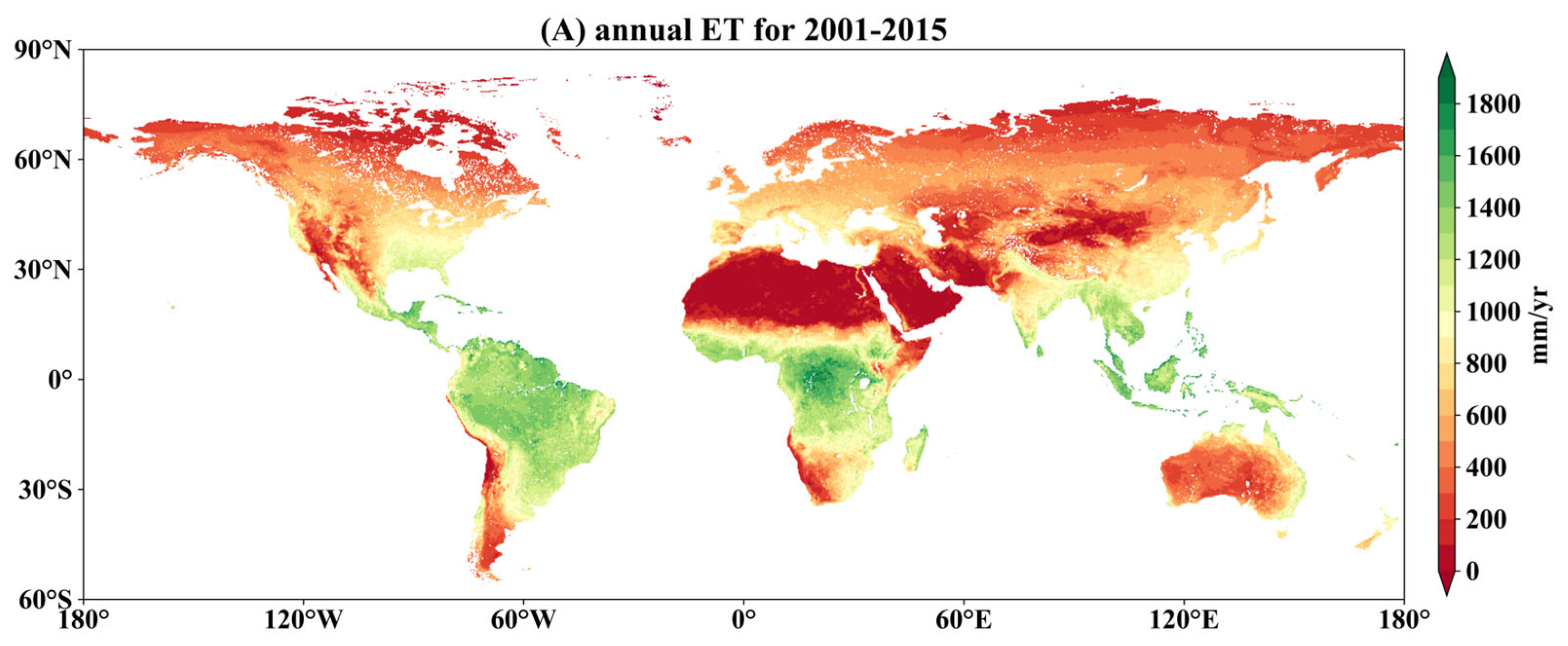
We applied the verified PML-SM model to the whole world for the period of 2001–2015 at a spatial resolution of 0.25°. Figure 1 shows the results of the mean annual ET, and coupled with ERA5 SM data over the period of 2001–2015. The mean annual ET distribution shows that high mean annual ET are found in densely vegetated humid areas such as the tropical rainforests of South America, central Africa and Southeast Asia. The low values of mean annual ET are concentrated in northern Africa, Central and West Asia, Australian desert areas, high latitudes and the west coast of North and South America. The lowest annual ET in these regions can be below 100 mm/yr. For , the high-value areas are concentrated in the rainforest areas near the equator, and the low-value areas are distributed similarly to ET. Low-value areas of are distributed in both tropical rainforest areas and arid desert areas. Tropical rainforest areas have low soil evaporation due to the dense vegetation cover all year round. Desert areas, on the other hand, have limited soil evaporation capacity due to the water shortage conditions.
3.3. Latitudinal Evolution
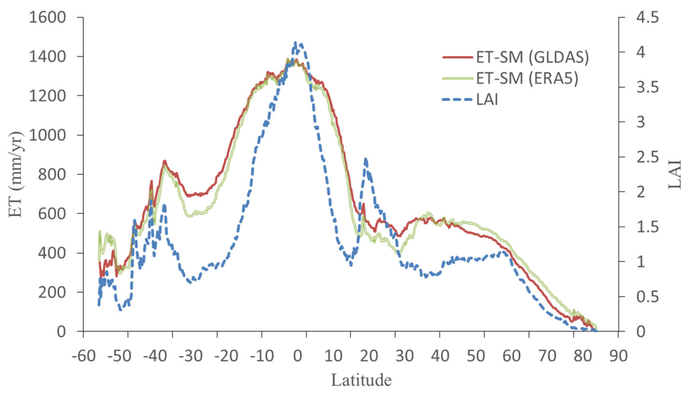
Figure 2 further explored the variation of annual ET features with latitude from a global scale. In general, the simulated results of coupling the two SM products showed relatively consistent distribution trends across the latitudinal zones. Rainforests are widespread near the equator and are the most evaporative region in the world due to abundant rain and heat and dense vegetation. These regions also have the highest LAI values in the world. At low and middle latitudes in the north and south latitudes, ET decreases overall. These areas are clearly controlled by the subtropical high-pressure zone with widespread deserts and distinct arid and low rainfall characteristics. In these regions, the simulation results of PML-SM (ERA5) are significantly lower than those of PML-SM (GLDAS). The prevailing westerly wind belt brings abundant ocean moisture to the mid-latitudes, and the average annual ET in these areas increases slightly. The increase in average annual ET is more pronounced in the mid-latitudes of the southern hemisphere, which may be influenced by two reasons. The first is that there is less land area in the mid-latitudes of the southern hemisphere; the second is that the land area of the northern hemisphere is extensive, and those inland far from the ocean have a predominantly continental climate with arid conditions that reduce ET. Annual ET is lowest at high latitudes, which is related to the lower temperature conditions in these regions.
4. Discussion
4.1. SM Constraint on and
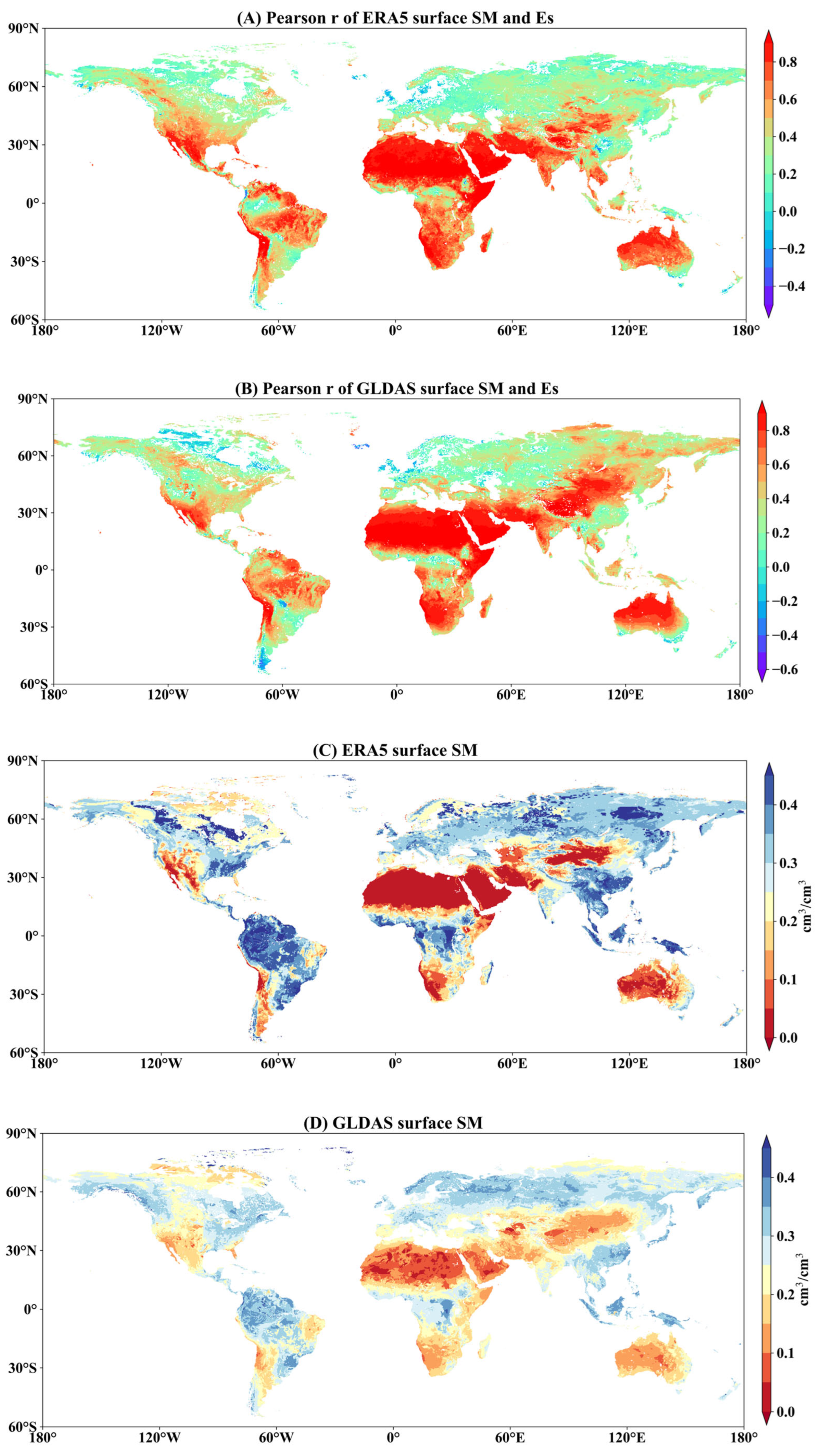
Although the effect of SM on ET has received attention from scholars, related research still needs further development due to the limitation of data conditions and other factors. In this paper, the correlation between SM and evaporation was further evaluated by introducing SM data into the soil evaporation and vegetation transpiration processes of the PML model. Figure 3 illustrates the distribution of ERA5, GLDAS SM data with Pearson r for and . Note that this paper only shows the correlation for regions with significance levels less than 0.05 [12]. Overall, the surface SM has a significant positive correlation with , while the negative correlation between SM in the root layer and is obvious.
Specifically, the simulation results of both coupled with ERA5 and GLDAS SM products reflect a predominantly positive relationship between land surface SM and . Dominant climatic characteristics may be an important factor in determining the strong correlation between SM and . The consistency of SM and is particularly evident in arid regions that are under the control of subtropical high pressure all year round, such as the North African region, the Arabian Peninsula, West Asia and the Australian continent. This is to some extent consistent with the findings of Rahmati et al. [37] on the relationship between ET and surface SM in arid regions. The regions controlled by tropical monsoon climate have distinct wet and dry seasons. The control of by SM in the dry season also makes the correlation higher in these regions. Examples include southern Africa, the Indian peninsula, and eastern South America. In particular, the correlation between SM and is also high in the interior of Asia and Europe, where the climate is dry all year round due to the long distance from the ocean. This is consistent with the view of similar studies that the effect of SM on ET is greater in areas subjected to greater soil moisture stress [38].
It should be noted that although the simulation results of coupling the two soil moisture data showed generally close spatial distribution characteristics, the correlation between soil moisture content and also showed different performance in local areas due to the differences between the two soil moisture data [39]. Within Asia and Europe, the results of coupled GLDAS SM have a much larger range of high values of correlation coefficients. In addition, the results of coupling this SM product show a more pronounced negative correlation at higher latitudes. The comparison of the two surface SM products also shows that although the spatial distribution trends of ERA5 and GLDAS surface SM are close, the SM values of GLDAS are lower than those of ERA5. This also implies that is relatively sensitive to the change range in the SM of the surface layer.
The relationship between SM in the root zone and is more complex. On a global scale, the correlation between these two elements includes both positive and negative characteristics. The relatively significant positive correlation feature appears in the Central African region. The distribution of the negative correlation characteristics is different due to the differences between the two SM data. As far as the results of coupled ERA5 SM are concerned, the negative correlation is more pronounced in the central–eastern part of Europe, whereas the results of coupled GLDAS SM have a relatively weaker negative correlation in the European region. The negative correlation between and SM in the root zone layer is enhanced in the high latitudes of North and South America and in Southeast Asia. Some relevant studies have shown a negative correlation between root layer SM and vegetation transpiration [37,40], but the relationship between the two elements is still a complex process influenced by multiple factors. The results in this paper may be related to some extent to the coupled simulation of SM. Even so, the simulation results based on the two SM products showed different correlation characteristics. Although is influenced by a variety of factors, this difference also arises to some extent in relation to the magnitude of the SM products in the two root zone layers. As can be seen in Figure 3G,H, the SM of the root zone layer is smaller for GLDAS [41].
4.2. Comparison with Other Global-Scale ET Simulation Studies
Many studies have carried out global-scale ET simulations [38,42,43] in which the coupling to SM has been considered to varying degrees [44]. We compared the simulation results of PML-SM with similar studies. In the comparison of the total annual amount of ET, the simulation results of PML-SM in this paper have close spatial distribution characteristics with those of Liu et al. [42] and are also consistent in terms of the maximum value of ET. After considering the interaction between SM and ET, the correlation between measured values and simulations is also strengthened [45]. In the distribution of different latitudes, the variation trend of ET simulated in this paper is also close to the research of Liu et al. [42]. However, compared with the global average annual ET maximum of 1500 mm [38,43,46], the maximum value of ET obtained by PML-SM in this paper is larger. Differences in data sources, reconstruction methods of remote sensing non-space-time continuous products, and coupling mechanisms between SM and ET processes are potential reasons for the different results of ET simulations.
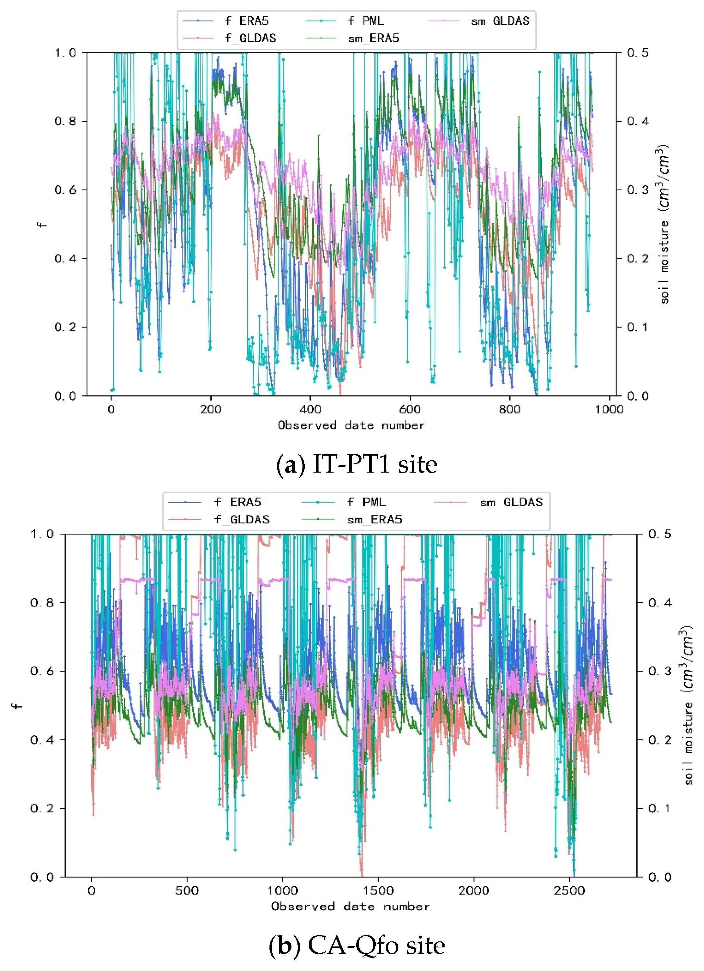
Since the differences between the PML-SM model constructed in this paper and other models are mainly reflected in the modification of the parameters and , the parameter variation process on the EC site can further reveal the reasons for the simulation results in this paper to some extent. Considering the complexity of the vegetation transpiration process, the comparison of the change process of some EC sites is shown here (Figure 4). Compared with the original parameterization scheme of the PML model [12], the parameterization results of the coupled SM are in better agreement with the variation of SM in the soil.
4.3. Limitations of This Study
The quality of SM data products is an important basis for conducting coupled ET and SM simulations. In this study, the differences in soil stratification between ERA5 and GLDAS products are not taken into consideration, while different root depths are not considered for different crop types [47], which may have an impact on the results. More refined research work is needed to follow up with spatial differences in crops.
The use and processing of remote sensing products is another issue that can continue to be improved. For the reconstruction of LAI products, this paper used the S-G filtering algorithm, which may bring some uncertainty to the spatial and temporal distribution of LAI data. Meanwhile, the temperature of the canopy surface is approximated by the surface temperature in this research, and the accuracy of the temperature products still needs to be improved subsequently.
The presence of the potential uncertainties mentioned above may introduce errors into the PML model parameters and the process of ET calculation, resulting in the new parameterization scheme not outperforming the original model at all sites. The simulation results present different RMSE accuracies for different land use types. The generalization of the canopy surface temperature, for example, has a potential impact on the calculation of , and the associated errors are optimized based on the physical mechanism of the parameter. This may, to some extent, affect the accuracy of the vegetation transpiration. Therefore, this preliminary research needs more studies to be refined.
5. Conclusions
By introducing land surface and root zone layer SM into the widely used PML model, this study conducted global ET simulations from 2001 to 2015. The comparison with the EC sites and similar studies shows that the simulation results of ET in this paper can further improve the correlation with the monitored values, meanwhile, the global spatial distribution is in good agreement with similar studies. The research further solidifies the physical mechanism of the PML model and strengthens the consistency between soil evaporation capacity and SM.
Comparing and with SM further reveals the influence of SM on ET processes on a global scale. Our results highlight that the adequate understanding of ET and reasonable portrayal of the interaction between the atmosphere and the soil during ET process is necessary. The relationship between two SM products, ERA5 and GLDAS, and ET is further analyzed to compare the differences between the two products in the simulation of ET. This study can provide further reference for the coupled simulation of ET and SM at a large scale, which is also useful for the mechanism analysis of water cycle process.
Limited by the data conditions, data generalization and interpolation methods, the simulation accuracy of ET needs to be further improved in subsequent studies. Optimizing the remote sensing data processing and validating the method on small scales for analysis are possible improvement directions.
Author Contributions
Conceptualization, H.D. and H.Z.; methodology, H.D. and H.X.; resources, Q.L.; data curation, C.H.; writing—original draft, H.D.; writing—review and editing, H.Z. All authors have read and agreed to the published version of the manuscript.
Funding
This research is supported by the National Key Research and Development Program of China (2021YFB3900602), the National Natural Science Foundation of China (52130907) and the Water Related Knowledge Service System (CKCEST-2022-1-35).
Data Availability Statement
The EC sites in this research are available from The Data Portal serving the FLUXNET community (https://fluxnet.org/ (accessed on 24 August 2021)). The ERA5 data used in this study are available from ECMWF (https://cds.climate.copernicus.eu/cdsapp#!/home (accessed on 29 July 2021)). The GLDAS soil moisture data are available from Earth Data (https://www.earthdata.nasa.gov/ (accessed on 22 October 2022)). The GLASS LAI data are available from http://www.glass.umd.edu/index.html (accessed on 28 May 2022).
Conflicts of Interest
The authors declare no conflict of interest.
References
- Khoshravesh, M.; Sefidkouhi, M.A.G.; Valipour, M. Estimation of reference evapotranspiration using multivariate fractional polynomial, Bayesian regression, and robust regression models in three arid environments. Appl. Water Sci. 2015, 7, 1911–1922. [Google Scholar] [CrossRef] [Green Version]
- Chirouze, J.; Boulet, G.; Jarlan, L.; Fieuzal, R.; Rodriguez, J.C.; Ezzahar, J.; Er-Raki, S.; Bigeard, G.; Merlin, O.; Garatuza-Payan, J.; et al. Intercomparison of four remote-sensing-based energy balance methods to retrieve surface evapotranspiration and water stress of irrigated fields in semi-arid climate. Hydrol. Earth Syst. Sci. 2014, 18, 1165–1188. [Google Scholar] [CrossRef] [Green Version]
- Mishra, V.; Kumar, R.; Shah, H.L.; Samaniego, L.; Eisner, S.; Yang, T. Multimodel assessment of sensitivity and uncertainty of evapotranspiration and a proxy for available water resources under climate change. Clim. Chang. 2017, 141, 451–465. [Google Scholar] [CrossRef]
- Li, S.; Wang, G.; Sun, S.; Fiifi Tawia Hagan, D.; Chen, T.; Dolman, H.; Liu, Y. Long-term changes in evapotranspiration over China and attribution to climatic drivers during 1980–2010. J. Hydrol. 2021, 595, 126037. [Google Scholar] [CrossRef]
- Cleugh, H.A.; Leuning, R.; Mu, Q.; Running, S.W. Regional evaporation estimates from flux tower and MODIS satellite data. Remote Sens. Environ. 2007, 106, 285–304. [Google Scholar] [CrossRef]
- Liu, G.; Liu, Y.; Hafeez, M.; Xu, D.; Vote, C. Comparison of two methods to derive time series of actual evapotranspiration using eddy covariance measurements in the southeastern Australia. J. Hydrol. 2012, 454–455, 1–6. [Google Scholar] [CrossRef]
- Zou, M.; Zhong, L.; Ma, Y.; Hu, Y.; Huang, Z.; Xu, K.; Feng, L. Comparison of Two Satellite-Based Evapotranspiration Models of the Nagqu River Basin of the Tibetan Plateau. J. Geophys. Res.-Atmos. 2018, 123, 3961–3975. [Google Scholar] [CrossRef]
- Gao, G.; Zhang, X.; Yu, T.; Liu, B. Comparison of three evapotranspiration models with eddy covariance measurements for a Populus euphratica Oliv. forest in an arid region of northwestern China. J. Arid Land 2015, 8, 146–156. [Google Scholar] [CrossRef] [Green Version]
- Jiang, L.; Islam, S. A methodology for estimation of surface evapotranspiration over large areas using remote sensing observations. Geophys. Res. Lett. 1999, 26, 2773–2776. [Google Scholar] [CrossRef] [Green Version]
- Gan, R.; Zhang, Y.; Shi, H.; Yang, Y.; Eamus, D.; Cheng, L.; Chiew, F.H.S.; Yu, Q. Use of satellite leaf area index estimating evapotranspiration and gross assimilation for Australian ecosystems. Ecohydrology 2018, 11, e1974. [Google Scholar] [CrossRef]
- Ma, N.; Zhang, Y. Increasing Tibetan Plateau terrestrial evapotranspiration primarily driven by precipitation. Agric. For. Meteorol. 2022, 317, 108887. [Google Scholar] [CrossRef]
- Zhang, Y.; Chiew, F.H.S.; Pena-Arancibia, J.; Sun, F.B.; Li, H.X.; Leuning, R. Global variation of transpiration and soil evaporation and the role of their major climate drivers. J. Geophys. Res.-Atmos. 2017, 122, 6868–6881. [Google Scholar] [CrossRef]
- Zhao, F.; Ma, S.; Wu, Y.; Qiu, L.; Wang, W.; Lian, Y.; Chen, J.; Sivakumar, B. The role of climate change and vegetation greening on evapotranspiration variation in the Yellow River Basin, China. Agric. For. Meteorol. 2022, 316, 108842. [Google Scholar] [CrossRef]
- Xing, W.; Wang, W.; Shao, Q.; Song, L.; Cao, M. Estimation of Evapotranspiration and Its Components across China Based on a Modified Priestley–Taylor Algorithm Using Monthly Multi-Layer Soil Moisture Data. Remote Sens. 2021, 13, 3118. [Google Scholar] [CrossRef]
- Qiu, J.; Crow, W.T.; Dong, J.; Nearing, G.S. Model representation of the coupling between evapotranspiration and soil water content at different depths. Hydrol. Earth Syst. Sci. 2020, 24, 581–594. [Google Scholar] [CrossRef] [Green Version]
- Morillas, L.; Leuning, R.; Villagarcía, L.; García, M.; Serrano-Ortiz, P.; Domingo, F. Improving evapotranspiration estimates in Mediterranean drylands: The role of soil evaporation. Water Resour. Res. 2013, 49, 6572–6586. [Google Scholar] [CrossRef]
- Teuling, A.J.; Seneviratne, S.I.; Williams, C.; Troch, P.A. Observed timescales of evapotranspiration response to soil moisture. Geophys. Res. Lett. 2006, 33, L23403. [Google Scholar] [CrossRef] [Green Version]
- Leuning, R.; Zhang, Y.Q.; Rajaud, A.; Cleugh, H.; Tu, K. A simple surface conductance model to estimate regional evaporation using MODIS leaf area index and the Penman-Monteith equation. Water Resour. Res. 2008, 44, W10419. [Google Scholar] [CrossRef]
- Duan, H.; He, X.; Zhao, H.; Jin, X.; Xu, H.; Wang, R. Analysis of the effect of seasonal changes on sensitive parameters of LAI-based Penman–Monteith evapotranspiration model based on particle swarm algorithm. Acta Geophys. 2022, 6, 1033–1043. [Google Scholar] [CrossRef]
- Li, F.; Cao, R.; Zhao, Y.; Mu, D.; Fu, C.; Ping, F. Remote sensing Penman–Monteith model to estimate catchment evapotranspiration considering the vegetation diversity. Theor. Appl. Climatol. 2015, 127, 111–121. [Google Scholar] [CrossRef]
- Wang, Q.M.; Jiang, S.; Zhai, J.Q.; He, G.H.; Zhao, Y.; Zhu, Y.N.; He, X.; Li, H.H.; Wang, L.Z.; He, F.; et al. Effects of vegetation restoration on evapotranspiration water consumption in mountainous areas and assessment of its remaining restoration space. J. Hydrol. 2022, 605, 127259. [Google Scholar]
- Zhang, Y.; Leuning, R.; Hutley, L.B.; Beringer, J.; McHugh, I.; Walker, J.P. Using long-term water balances to parameterize surface conductances and calculate evaporation at 0.05° spatial resolution. Water Resour. Res. 2010, 46, W05512. [Google Scholar] [CrossRef] [Green Version]
- Feng, J.; Zhang, K.; Zhan, H.; Chao, L. Improved soil evaporation remote sensing retrieval algorithms and associated uncertainty analysis on the Tibetan Plateau. Hydrol. Earth Syst. Sci. 2023, 27, 363–383. [Google Scholar] [CrossRef]
- Noilhan, J.; Planton, S. A simple parameterization of land surface processes for meteorological models. Mon. Weather Rev. 1989, 117, 536–549. [Google Scholar] [CrossRef]
- Ben Mehrez, M.; Taconet, O.; Vidal-Madjar, D.; Valencogne, C. Estimation of stomatal resistance and canopy evaporation during the HAPEX-MOBILHY experiment. Agric. For. Meteorol. 1992, 58, 285–313. [Google Scholar] [CrossRef]
- Xing, Z.; Fan, L.; Zhao, L.; De Lannoy, G.; Frappart, F.; Peng, J.; Li, X.; Zeng, J.; Al-Yaari, A.; Yang, K.; et al. A first assessment of satellite and reanalysis estimates of surface and root-zone soil moisture over the permafrost region of Qinghai-Tibet Plateau. Remote Sens. Environ. 2021, 265, 112666. [Google Scholar] [CrossRef]
- Liang, S.; Cheng, J.; Jia, K.; Jiang, B.; Liu, Q.; Xiao, Z.; Yao, Y.; Yuan, W.; Zhang, X.; Zhao, X.; et al. The Global Land Surface Satellite (GLASS) Product Suite. Bull. Am. Meteorol. Soc. 2021, 102, E323–E337. [Google Scholar] [CrossRef]
- Liang, S.; Zhang, X.; Xiao, Z.; Cheng, J.; Liu, Q.; Zhao, X. Global Land Surface Satellite (GLASS) Products: Algorithms, Validation and Analysis; Springer: Berlin/Heidelberg, Germany, 2013. [Google Scholar]
- Liang, S.; Zhao, X.; Liu, S.; Yuan, W.; Cheng, X.; Xiao, Z.; Zhang, X.; Liu, Q.; Cheng, J.; Tang, H.; et al. A long-term Global LAnd Surface Satellite (GLASS) data-set for environmental studies. Int. J. Digit. Earth 2013, 6, 5–33. [Google Scholar] [CrossRef]
- Chen, J.; Jönsson, P.; Tamura, M.; Gu, Z.; Matsushita, B.; Eklundh, L. A simple method for reconstructing a high-quality NDVI time-series data set based on the Savitzky–Golay filter. Remote Sens. Environ. 2004, 91, 332–344. [Google Scholar] [CrossRef]
- Zheng, J.; Zhao, T.; Lü, H.; Shi, J.; Cosh, M.H.; Ji, D.; Jiang, L.; Cui, Q.; Lu, H.; Yang, K.; et al. Assessment of 24 soil moisture datasets using a new in situ network in the Shandian River Basin of China. Remote Sens. Environ. 2002, 271, 112891. [Google Scholar] [CrossRef]
- Bi, H.; Ma, J.; Zheng, W.; Zeng, J. Comparison of soil moisture in GLDAS model simulations and in situ observations over the Tibetan Plateau. J. Geophys. Res.-Atmos. 2016, 121, 2658–2678. [Google Scholar] [CrossRef] [Green Version]
- Cai, J.; Zhang, Y.; Li, Y.; Liang, X.; Jiang, T. Analyzing the Characteristics of Soil Moisture Using GLDAS Data: A Case Study in Eastern China. Appl. Sci. 2017, 7, 566. [Google Scholar] [CrossRef] [Green Version]
- Kędzior, M.; Zawadzki, J. Comparative study of soil moisture estimations from SMOS satellite mission, GLDAS database, and cosmic-ray neutrons measurements at COSMOS station in Eastern Poland. Geoderma 2016, 283, 21–31. [Google Scholar] [CrossRef]
- Cui, Y.; Tan, J.; Jing, W.; Tan, G. Applicability evaluation of merged soil moisture in GLDAS and CLDAS products over Qinghai-Tibetan Plateau. Plateau Meteorol. 2018, 37, 123–136. [Google Scholar]
- Pastorello, G.; Trotta, C.; Canfora, E.; Chu, H.; Christianson, D.; Cheah, Y.W.; Poindexter, C.; Chen, J.; Elbashandy, A.; Humphrey, M.; et al. The FLUXNET2015 dataset and the ONEFlux processing pipeline for eddy covariance data. Sci. Data 2020, 7, 225. [Google Scholar] [CrossRef]
- Rahmati, M.; Groh, J.; Graf, A.; Pütz, T.; Vanderborght, J.; Vereecken, H. On the impact of increasing drought on the relationship between soil water content and evapotranspiration of a grassland. Vadose Zone J. 2020, 19, e20029. [Google Scholar] [CrossRef]
- Yan, H.; Wang, S.Q.; Billesbach, D.; Oechel, W.; Zhang, J.H.; Meyers, T.; Martin, T.A.; Matamala, R.; Baldocchi, D.; Bohrer, G.; et al. Global estimation of evapotranspiration using a leaf area index-based surface energy and water balance model. Remote Sens. Environ. 2012, 124, 581–595. [Google Scholar] [CrossRef] [Green Version]
- Wu, Z.; Feng, H.; He, H.; Zhou, J.; Zhang, Y. Evaluation of soil moisture climatology and anomaly components derived from ERA5-Land and GLDAS-2.1 in China. Water Resour. Manag. 2021, 35, 629–643. [Google Scholar] [CrossRef]
- Williams, I.N.; Torn, M.S. Vegetation controls on surface heat flux partitioning, and land-atmosphere coupling. Geophys. Res. Lett. 2015, 42, 9416–9424. [Google Scholar] [CrossRef]
- Yang, S.; Zeng, J.; Fan, W.; Cui, Y. Evaluating root-zone soil moisture products from GLEAM, GLDAS, and ERA5 based on in situ observations and triple collection method over Tibetan Plateau. J. Hydrometeorol. 2022, 23, 1861–1878. [Google Scholar] [CrossRef]
- Liu, Y.; Jiang, Q.; Wang, Q.; Jin, Y.; Yue, Q.; Yu, J.; Zheng, Y.; Jiang, W.; Yao, X. The divergence between potential and actual evapotranspiration: An insight from climate, water, and vegetation change. Sci. Total Environ. 2022, 807 Pt 1, 150648. [Google Scholar] [CrossRef] [PubMed]
- Zhang, Y.; Kong, D.; Gan, R.; Chiew, F.H.S.; McVicar, T.R.; Zhang, Q.; Yang, Y. Coupled estimation of 500 m and 8-day resolution global evapotranspiration and gross primary production in 2002–2017. Remote Sens. Environ. 2019, 222, 165–182. [Google Scholar] [CrossRef]
- Purdy, A.J.; Fisher, J.B.; Goulden, M.L.; Colliander, A.; Halverson, G.; Tu, K.; Famiglietti, J.S. SMAP soil moisture improves global evapotranspiration. Remote Sens. Environ. 2018, 219, 1–14. [Google Scholar] [CrossRef]
- Hssaine, B.A.; Merlin, O.; Rafi, Z.; Ezzahar, J.; Jarlan, L.; Khabba, S.; Er-Raki, S. Calibrating an evapotranspiration model using radiometric surface temperature, vegetation cover fraction and near-surface soil moisture data. Agric. For. Meteorol. 2018, 256–257, 104–115. [Google Scholar] [CrossRef] [Green Version]
- Ma, N.; Szilagyi, J.; Zhang, Y. Calibration-Free Complementary Relationship Estimates Terrestrial Evapotranspiration Globally. Water Resour. Res. 2021, 57, e2021WR029691. [Google Scholar] [CrossRef]
- Cui, Y.; Jia, L. Estimation of evapotranspiration of “soil-vegetation” system with a scheme combining a dual-source model and satellite data assimilation. J. Hydrol. 2021, 603, 127145. [Google Scholar] [CrossRef]
Figure 1.
Spatial distribution map of multi–year annual ET (A), (B) and (C).


Figure 2.
The variation of ET with latitude in multi−year average value.

Figure 3.
Spatial distribution of Pearson r of SM and ET components.


Figure 4.
The variation process of obtained by different methods and SM values.


Table 1.
Basic information of EC sites used in this study.
| Site ID | Climate | Years | Vegetation | Mean Annual Precipitation (mm) |
|---|---|---|---|---|
| AT-Neu | warm summer continental | 2002–2012 | grassland | 852 |
| AU-DaS | tropical savanna | 2008–2014 | savannas | 975.82 |
| CA-Qfo | subarctic | 2003–2010 | evergreen needleleaf forests | 962.32 |
| CA-SF1 | subarctic | 2003–2006 | evergreen needleleaf forests | 470 |
| CA-SF2 | subarctic | 2002–2005 | evergreen needleleaf forests | 470 |
| CH-Cha | warm summer continental | 2006–2012 | mixed forests | 663.59 |
| CN-HaM | tundra | 2002–2004 | grasslands | - |
| FI-Hyy | subarctic | 2004–2014 | evergreen needleleaf forests | 709 |
| FI-Lom | subarctic | 2007–2009 | permanent wetlands | 484 |
| FI-Sod | - | 2002–2010 | evergreen needleleaf forests | 500 |
| IT-PT1 | - | 2002–2004 | deciduous broadleaf forests | 984 |
| US-Me5 | Mediterranean | 2000–2002 | evergreen needleleaf forests | 590.81 |
| US-Syv | warm summer continental | 2001–2008 | mixed forests | 826 |
Table 2.
Quantitative measures of the PML model, PML-SM model performance at daily time-steps for 13 EC sites.
Table 2.
Quantitative measures of the PML model, PML-SM model performance at daily time-steps for 13 EC sites.
| EC Site | PML-SM (ERA5) Model | PML-SM (GLDAS) Model | PML Model | |||
|---|---|---|---|---|---|---|
| Pearson r | RMSE (mm/d) | Pearson r | RMSE (mm/d) | Pearson r | RMSE (mm/d) | |
| AT-Neu | 0.89 | 1.30 | 0.89 | 1.23 | 0.90 | 1.00 |
| AU-DaS | 0.89 | 1.78 | 0.87 | 1.75 | 0.72 | 0.87 |
| CA-Qfo | 0.86 | 1.80 | 0.86 | 1.71 | 0.72 | 1.59 |
| CA-SF1 | 0.87 | 1.77 | 0.60 | 1.48 | 0.77 | 1.44 |
| CA-SF2 | 0.85 | 1.69 | 0.83 | 1.54 | 0.67 | 1.22 |
| CH-Cha | 0.88 | 1.95 | 0.55 | 1.56 | 0.68 | 1.68 |
| CN-HaM | 0.80 | 1.56 | 0.65 | 1.21 | 0.74 | 0.99 |
| FI-Hyy | 0.92 | 1.59 | 0.89 | 1.51 | 0.88 | 1.29 |
| FI-Lom | 0.91 | 1.46 | 0.89 | 1.39 | 0.85 | 1.09 |
| FI-Sod | 0.89 | 1.43 | 0.86 | 1.38 | 0.82 | 0.98 |
| IT-PT1 | 0.73 | 1.87 | 0.70 | 1.22 | 0.60 | 1.32 |
| US-Me5 | 0.71 | 1.01 | 0.78 | 1.11 | 0.30 | 0.61 |
| US-Syv | 0.71 | 2.04 | 0.69 | 2.01 | 0.60 | 1.74 |
Disclaimer/Publisher’s Note: The statements, opinions and data contained in all publications are solely those of the individual author(s) and contributor(s) and not of MDPI and/or the editor(s). MDPI and/or the editor(s) disclaim responsibility for any injury to people or property resulting from any ideas, methods, instructions or products referred to in the content. |
© 2023 by the authors. Licensee MDPI, Basel, Switzerland. This article is an open access article distributed under the terms and conditions of the Creative Commons Attribution (CC BY) license (https://creativecommons.org/licenses/by/4.0/).
Share and Cite
MDPI and ACS Style
Duan, H.; Zhao, H.; Li, Q.; Xu, H.; Han, C. Estimation of Evapotranspiration Based on a Modified Penman–Monteith–Leuning Model Using Surface and Root Zone Soil Moisture. Water 2023, 15, 1418. https://doi.org/10.3390/w15071418
AMA Style
Duan H, Zhao H, Li Q, Xu H, Han C. Estimation of Evapotranspiration Based on a Modified Penman–Monteith–Leuning Model Using Surface and Root Zone Soil Moisture. Water. 2023; 15(7):1418. https://doi.org/10.3390/w15071418
Chicago/Turabian StyleDuan, Hao, Hongli Zhao, Qiuju Li, Haowei Xu, and Chengxin Han. 2023. "Estimation of Evapotranspiration Based on a Modified Penman–Monteith–Leuning Model Using Surface and Root Zone Soil Moisture" Water 15, no. 7: 1418. https://doi.org/10.3390/w15071418
Note that from the first issue of 2016, this journal uses article numbers instead of page numbers. See further details here.