
Improvement of Hargreaves–Samani Reference Evapotranspiration Estimates in the Peruvian Altiplano

1
Programa de Maestría en Riego y Drenaje, Universidad Nacional Agraria La Molina, Lima 15024, Peru
2
Escuela Profesional de Ingeniería Agrícola, Universidad Nacional del Altiplano, Puno 21001, Peru
*
Author to whom correspondence should be addressed.
Water 2023, 15(7), 1410; https://doi.org/10.3390/w15071410
Submission received: 30 January 2023
/
Revised: 1 March 2023
/
Accepted: 15 March 2023
/
Published: 5 April 2023
(This article belongs to the Special Issue Crop Evapotranspiration: Accurate Ground and Remote Sensing Observations and Computational Tools)
Abstract
:The FAO 56 Penman–Monteith equation (PM) is considered the most accurate method for estimating reference evapotranspiration (ETo). However, PM requires a large amount of data that is not always available. Thus, the objective of this study is to improve the Hargreaves–Samani (HS) reference evapotranspiration estimates in the Peruvian Altiplano (PA) by calibrating the radiation coefficient KRS. The results show modified HS (HSM) ETo estimates at validation after KRS calibration, revealing evident improvements in accuracy with Nash–Sutcliffe efficiency (NSE) between 0.58 and 0.93, percentage bias (PBIAS) between −0.58 and 1.34%, mean absolute error (MAE) between −0.02 and 0.05 mm/d, and root mean square error (RMSE) between 0.14 and 0.25 mm/d. Consequently, the multiple linear regression (MLR) model was used to regionalize the KRS for the PA. It is concluded that, in the absence of meteorological data, the HSM equation can be used with the new values of KRS instead of HS for the PA.
1. Introduction
Reference evapotranspiration (ETo) is one of the most useful and necessary indicators for efficient irrigation management [1]. The ETo plays an important role in estimating the water requirements of crops and irrigation programming, irrigation and drainage design, as well as drought management and studies related to climate change and variation [2,3,4,5]. Crop coefficients, which depend on crop characteristics and local conditions, are used to convert ETo into actual crop evapotranspiration ETr [6], with accurate estimation of ETo being of great importance.
In situ measurement of ETo is expensive and time consuming, and is subject to significant uncertainties. Due to the limitation of in situ measurements of ETo, several empirical models have been developed for its estimation [7]. The empirical models for ETo estimation available in the scientific literature are classified as (1) combination models completely based on physics that explain the principles of conservation of mass and energy; (2) semi-physical models that deal with the conservation of mass or energy; and (3) black box models based on artificial neural networks, empirical relationships, and fuzzy and genetic algorithms [8,9,10,11].
The method recommended to estimate ETo by the Food and Agriculture Organization of the United Nations (FAO) is the FAO Penman–Monteith equation 56 (PM) [6,12,13]. ETo is defined as the evapotranspiration rate of a hypothetical reference crop with an assumed crop height of 0.12 m, a surface resistance of 70 s/m and an albedo of 0.23, very similar to the evapotranspiration of a large area. green grass of uniform height, actively growing, completely shading the ground and not lacking in water [13]. Therefore, the PM equation is written as:
where is the reference evapotranspiration (mm/d), is the slope of the vapor pressure curve (Kpa/°C), is the net radiation on the crop surface (MJ/m2/d), is the soil heat flux density (MJ/m2/d), is the mean air temperature (°C), is the mean wind speed at a height 2 m (m/s), is the saturation vapor pressure (kPa), is the actual vapor pressure (kPa), is the vapor pressure deficit (kPa) and is the psychrometric constant (kPa/°C).
The PM equation was classified as the best to estimate ETo in all types of weather, it can be used globally without any local calibration, since it incorporates physiological and aerodynamic parameters, and has been tested using a variety of lysimeters [1,13]. PM works well in different regions of the world with data on air temperature, relative humidity, solar radiation, and wind speed [14]. However, in places with low availability of meteorological data, its application becomes limited, being the main impediment for the widespread use of the PM equation, therefore, alternative approaches are required to calculate the ETo.
Data limitations motivated Hargreaves and Samani [15] to develop an alternative approach to estimate ETo using only air temperature and extraterrestrial solar radiation data. For this reason, when the necessary meteorological data are not available for the calculation of ETo by the PM method, the Hargreaves–Samani (HS) method is recommended. Due to its simple application for the calculation of ETo with temperature data alone, the focus of research has been the use of the Hargreaves–Samani (HS) equation [15]. This equation can be written as:
where, corresponds to the reference evapotranspiration of the grass (mm/d), is the extraterrestrial radiation (mm/d), , y is the maximum, minimum and average temperature (°C), 0.0135 is a conversion factor of units from the American System to the International System, is the adjustment coefficient of the empirical radiation (°C−0.5), and 17.8 is an empirical factor related to the temperature units used in the original formulations.
The empirical coefficient was initially set at 0.17 °C−0.5 for arid and semi-arid regions [16]. According to Allen et al. [13], the adjustment coefficient differs for inland or coastal regions, thus, for inland locations where land mass dominates or next to it and where air masses are influenced by a nearby water mass, = 0.16 °C−0.5, while for coastal locations with or adjacent to a large land mass where air masses are influenced by a nearby water mass, = 0, 19 °C−0.5. With in mm/day and the empirical coefficient is normally considered as 0.17 °C−0.5.
Studies carried out under different climatic conditions reported that the calibration of the equations based on air temperature and radiation improved performance [17,18,19]. In effect, in the scientific literature, various studies worldwide adjusted the coefficients of the original HS equation to improve performance, they also included monthly precipitation [2], for different climatic zones [16], in specific geographic regions regional and local calibration [1,6,17,20,21,22,23,24,25], others included the altitude of the sites as a variable [26,27], related to the calibration of the radiation coefficient () [5,28,29,30]. Therefore, it is very important to investigate the coefficient of radiation () to reduce the estimation error of the original HS equation, at high altitude and under conditions of the Peruvian Altiplano (PA).
Since the calibration of the of the HS equation can improve the estimates of ETo, we focus this investigation on the main question: Is it possible to improve the reference evapotranspiration estimates of HS in the Peruvian Altiplano? To provide reasonable answers, this article focuses on the principal objective of improving the reference evapotranspiration estimates in the PA through a calibration of the radiation coefficient KRS of the HS equation, under environmental conditions of the PA, and as specific objectives (1) evaluate the original HS equation, (2) calibrate and validate the radiation coefficient KRS of the HS equation, and (3) regionalize the radiation coefficient for the PA based on the geographic characteristics.
2. Materials and Method
2.1. Study Area
The study area is located in the Peruvian Lake Titicaca basin (PLTB). It is characterized as an endorheic basin system surrounded by the eastern and western mountain ranges. It limits to the north with the Amazon hydrographic region, to the south-west with the Pacific hydrographic region and to the east with the PLT of the Republic of Bolivia, with an altitude (Figure 1a) that varies from 3804 to 5781 m.a.s.l. According to the climatic classification of Peru, the PLT has a predominantly rainy climate type, with dry autumn and winter [31].
The study area has an average annual rainfall that varies from 624.9 mm to 948.3 mm. The maximum and minimum air temperatures for all seasons range between 10.5 and 17.8 °C, and −2.2 and 3.5 °C, respectively. The relative humidity varies between 55% and 80.6%, while the wind speed oscillates between 1.5 and 5.5 m/s. The sun hours are between 6.3 and 8.4 h, and the altitudes of the stations are between 3812 and 4660 m.a.s.l. On the other hand, the aridity index (AI) for the meteorological station sites varies between 0.54 and 0.78 (mean 0.64). The AI is defined as the relationship between the annual precipitation (P) and the annual reference evapotranspiration (ETo) [32]. Then, the weather station sites are climatically classified as dry sub-humid (SH-s) to humid sub-humid (SH-h) (Table 1) according to the AI levels defined for Peru by Huerta and Lavado [32].
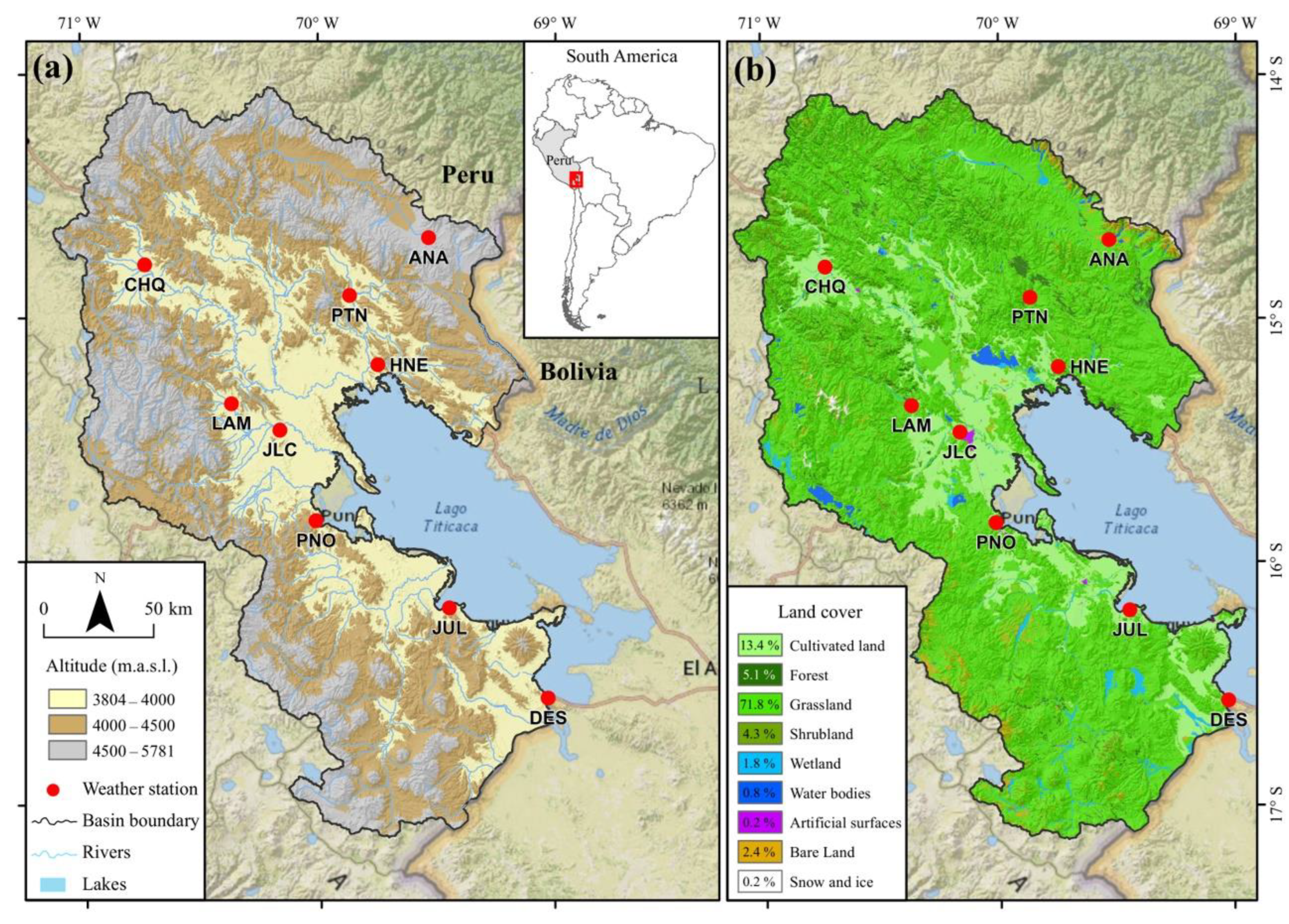
According to GlobeLand30 version 2010, the dominant land cover type for the PA is grassland, followed by cultivated land, forest, shrubland, bare land, wetland, water bodies, snow and ice, and artificial surfaces. GlobeLand30 is a 30 m spatial resolution global land cover data product developed by China [33], with versions available for 2000, 2010 and 2020 (http://www.globallandcover.com: accessed on 16 February 2023). Most weather stations are located on grassland (PTN, JLC and PNO), cultivated land (CHQ, HNE and JUL) and Artificial surfaces (ANA and DES) (Figure 1b).
2.2. Climatic and Terrain Data
The data used for this study are monthly values of maximum (Tmax, °C) and minimum (Tmin, °C) air temperature, relative humidity (RH, %), sun hours (SH, h), wind speed (U10, m/s) at a height of 10 m and precipitation (P, mm) from nine weather stations distributed in the PA (Figure 1a). The selected stations have data records from 2000 to 2019 (information provided by the National Meteorology and Hydrology Service of Peru (SENAMHI)). The stations considered include the representative stations of the PA, defined on the basis of the aridity index suggested by Huerta and Lavado [32].
A quality control process of the rain gauge measurements was carried out, which consisted of the verification of specific physical limits for the Peruvian territory, internal consistency, and spatial consistency [34]. The homogeneity of the climatic variables Rh, U10, Sh, Tmax, Tmin and P were analyzed by means of a visual inspection, and the absolute method. For the absolute method, the nonparametric test of Distribution-free cumulative sum (CUSUM) and rank-sum (RS) were applied independently to the data from each weather station using the TREND program (https://toolkit.ewater.org.au/Tools/TREND: accessed on 10 August 2022). CUSUM, is a nonparametric test of step jump in the mean, while RS is a nonparametric test of difference in the mean of two periods [35]. The null hypothesis for CUSUM and RS suggests that there is no step jump in the mean in the data series, and there is no difference in the mean between two data periods, which accepts the null hypothesis if the maximum deviation for CUSUM and the statistic z for calculated RS are less than the critical value of the statistical table at the 5% significance level and rejects it otherwise. Thus, the doubtful periods of the Rh, U10, Sh, Tmax, Tmin and P data series that did not meet the assumption of homogeneity were not considered in subsequent analyses.
In effect, the missing values were filled in using the random forest (RF) machine learning algorithm incorporated in the MICE (Generates Multivariate Imputations by Chained Equations) package for the R project [36]. It should be noted that the homogeneity of the data was checked with monthly data after filling in the missing data [37,38]. Homogeneity tests are generally more robust when used with monthly data [37]. The wind speed at a height of 2 m (U2, m/s) was calculated from U10.
Lat south latitude; Long west longitude; Alt altitude (m.a.s.l.); Rh relative humidity (%); U2 wind speed (m/s) at a height of 2 m; Sh sun hours (h); ETo reference evapotranspiration estimated by the PM method (mm/d); P annual precipitation (mm/year); AI aridity index; CC climatic classification; SH-h subhumid-humid; SH-d subhumid-dry.
To regionalize the KRS radiation coefficient calibrated from the HS equation, the NASA Shuttle Radar Topography Mission (SRTM) digital elevation model (DEM) was obtained from the Google Earth Engine (GEE) platform available at https://earthengine.google.com/ (accessed on 15 July 2022), ID de la imagen CGIAR/SRTM90_V4 [39], with a spatial resolution of ~90 m.
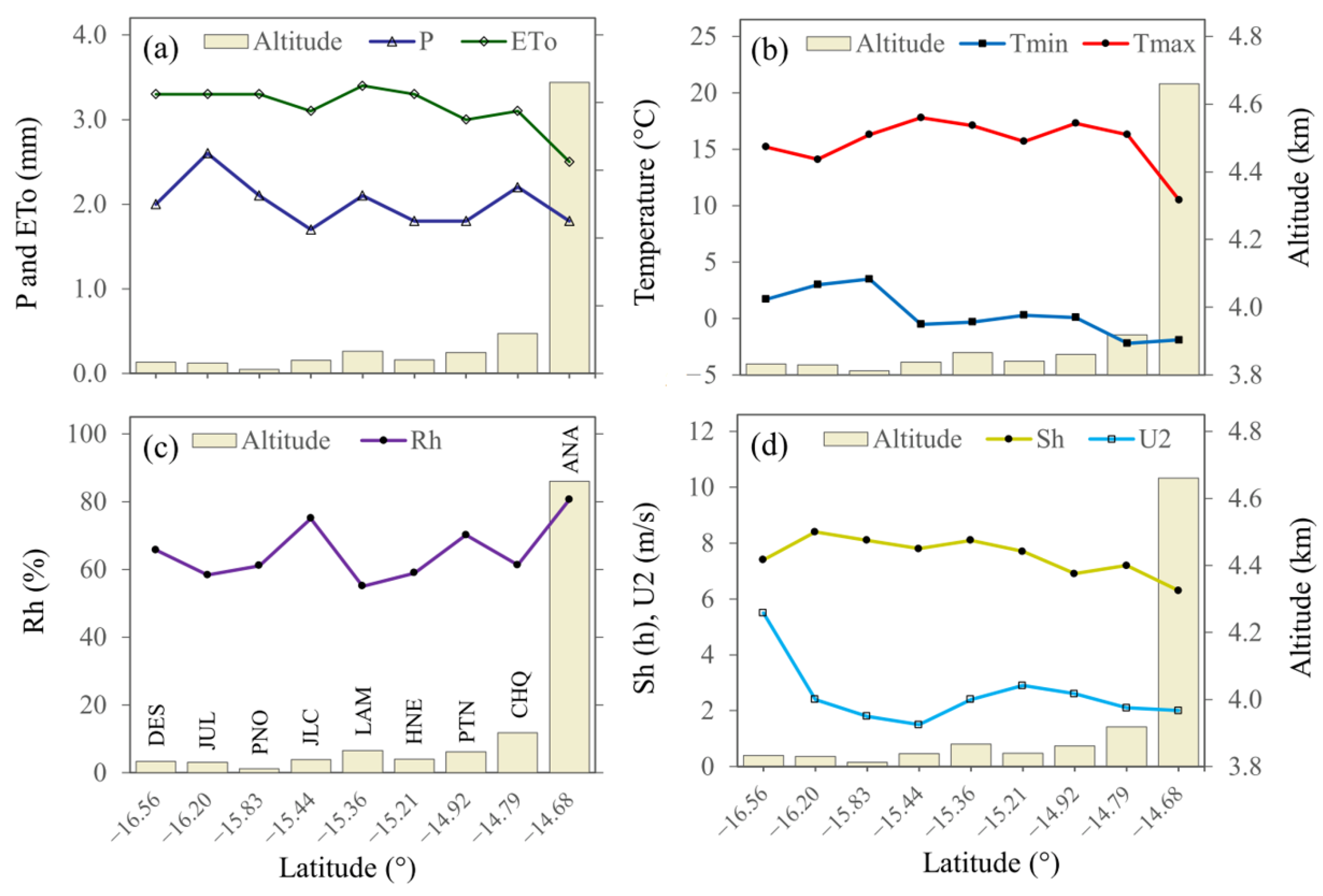
Figure 2 shows that the climatic and geographical variables that affect the ETo. As the altitude increases, precipitation, reference evapotranspiration, minimum and maximum temperature, sun hours and wind speed decrease, on the contrary, relative humidity increases, for the weather stations under study.
2.3. Evaluation of the Original Hargreaves-Samani Equation for Use in the Peruvian Altiplano
In this study, the PM method has been used as a substitute for reference evapotranspiration measured data, being the standard procedure when no lysimeter measured data is available [20]. Due to the lack of experimental reference evapotranspiration (ETo) measurements, the numbers given by the PM equation have been accepted as the true values. Moreover, this equation has been used to calibrate the modified versions of the Hargreaves–Samani (HS) equations [13,16].
The calculation of all the data required for the estimation of the ETo followed the recommendations given in the manual 56 of Irrigation and Drainage of the FAO [6].
where is the extraterrestrial radiation (MJ/m2/d), is the actual duration of sunlight (h), is the maximum possible duration of sunlight or hours of sunlight (h), is the regression constant which expresses the fraction of extraterrestrial radiation that reaches the earth on cloudy days ) and is the fraction of extraterrestrial radiation that reaches the earth on clear days ). In the absence of real measurements and calibration of solar radiation , values suggested by Allen et al. [13] are and . However, these default values should not be applied to high altitude sites, where proper calibration is required [40]. In this regard, values of and suggested by Chipana et al. [3], were used for high altitude areas (3820 to 3950 m.a.s.l.) estimated for the Bolivian altiplano and for altitudes above the 4660 m.a.s.l was considered with slight modifications of and .
Extraterrestrial radiation was estimated using the equation recommended by Allen et al. [13]. The values of for each day of the year and for different latitudes can be estimated from the solar constant, the solar declination and the time of the year and then selecting the for the 15th day of each month converted to monthly values, using the following equation:
where is the solar constant = 0.0820 MJ/m2/min, is the inverse relative distance to the sun, is the hour angle of sunset (rad), is the latitude (rad), and is the solar declination (rad).
The net radiation was calculated as the difference between the incoming net shortwave radiation and the outgoing net longwave radiation .
To calculate the net incoming shortwave radiation , the value used for albedo was 0.23, while the net longwave radiation , was estimated using the expression postulated by the modified Stefan-Boltzmann law due to absorption and downward radiation from the sky [13].
where is the net longwave radiation (MJ/m2/d), is the Stefan-Boltzmann constant (4.903 × 10⁻⁹ MJ/K−4/m2/d), is the maximum absolute temperature during the 24 h period (K = °C + 273), is the minimum absolute temperature during the 24 h period (K = °C + 273), is the actual vapor pressure (kPa), is the relative shortwave radiation (limited a ≤ 1.0), is the calculated solar radiation (MJ/m2/d) and is the calculated clear-sky radiation (MJ/m2/d).
The vapor pressure deficit is calculated as the difference between the saturation vapor pressure and the actual vapor pressure . is calculated as the average of the saturation vapor pressure at and . Approximations can be used to estimate depending on the available data. When only daily mean relative humidity data is available, is calculated as [13]:
2.4. Statistical Performance Metrics
To evaluate the performance between the original HS and the PM method for the nine weather stations, statistical performance metrics were used (Table 2), including the correlation coefficient (R), the Nash–Sutcliffe efficiency coefficient (NSE) used by Almorox and Grieser [16] and Todorovic et al. [4], percent bias (PBIAS), and root mean square error (RMSE) and mean absolute error (MAE), both used by Cobaner et al. [25].
The R denotes the degree of correlation between the observed and calculated values of ETo, with values ranging from −1.0 to 1.0, where values closer to ±1 indicate a better association between them. Legates and McCabe [41] suggest using the NSE coefficient to assess goodness of fit. [42] defined the coefficient of efficiency ranging from minus infinity to 1.0, where higher values indicate a better relationship. The NSE indicates that when the residual variance is equal to the variance of the observed data, the result is NSE = 1.0. On the contrary, when the NSE is equal to zero or is negative, it indicates that the observed mean is as good or a better predictor than the model. [43] classified the performance of a model as very good if NSE > 0.75, good if 0.65 < NSE ≤ 0.75, satisfactory if 0.50 < NSE ≤ 0.65 and poor if NSE ≤ 0.50.
Instead, PBIAS indicates the average trend of simulated data based on larger or smaller observed data, with the best value being 0 and negative (positive) values indicating an underestimation (overestimation) [44]. According to the criteria of Moriasi et al. [45], the statistical performance of models can be considered ‘very good’ when PBIAS < ±5, ‘good’ when ±5 ≤ PBIAS < ±10, ‘satisfactory’ when ±10 ≤ PBIAS < ±25 and ‘not satisfactory’ when PBIAS ≥ ±25.
On the other hand, [46] indicate that the MAE is the most natural measure of the magnitude of the average error of the absolute differences between what is observed and calculated. A low MAE value implies a high performance of the model. Meanwhile, the RMSE is one of the commonly used error rates [16], and it follows that a smaller RMSE indicates a better approximation of the model.
2.5. Calibration and Validation of the Radiation Coefficient KRS of the HS Equation
Todorovic et al. [4] reported that it is preferable to adjust the values of than to change the coefficient of 0.0023. Under this perspective, the HS equation was modified by means of calibrating the expressed as:
The of the HS equation was adjusted using the ETo data determined by the PM method, and was calibrated using the generalized reduced gradient (GRG) non-linear resolution method of the Microsoft Excel Solver tool. To define the objective function, the maximization of the ENS function (Nash–Sutcliffe coefficient of efficiency) and the minimization of the RMSE function (root mean square error) were established as the optimization objective in the Solver tool.
Shiri et al. [47] report that testing the calibrated version using the same calibration data could lead to partially valid results. Therefore, the observed data corresponding to the period from 2000 to 2019 were separated into two groups, being considered for calibration (70%) and validation (30%). However, using historical data to calibrate the HS model directly ignores the continuity of climate change over time, which can lead to good performance of the calibrated HS model in the calibrated years; however, instability may appear when the HS model is an extended data set [48]. To reduce this instability, the calibration and validation period was selected randomly. Consequently, to verify the validity of the new obtained from the HS equation, they were evaluated through performance metrics, which that include the ENS, PBIAS, MAE and RMSE (Table 2).
2.6. Regionalization of the Radiation Coefficient
A geographic information system (GIS) was used to spatially interpolate the point values of at a spatial resolution of ~90 m. The multiple linear regression (MLR) method was used with as the dependent variable, while the longitude, latitude and altitude were used as independent variables followed by residual values. The longitude and latitude maps were interpolated using the inverse distance weighted (IDW) method based on the pixel centroids of the altitude map, while the residue map was interpolated using the IDW method based on point location values of each weather station. Next, was obtained using map algebra (raster calculator tool) in ArcGIS. The value of at the unmeasured points is obtained according to the following equation:
where: is the predicted value at point , are the MRL coefficients, the values of are the independent variables at point , is the longitude, is the latitude, is the altitude, and the residue.
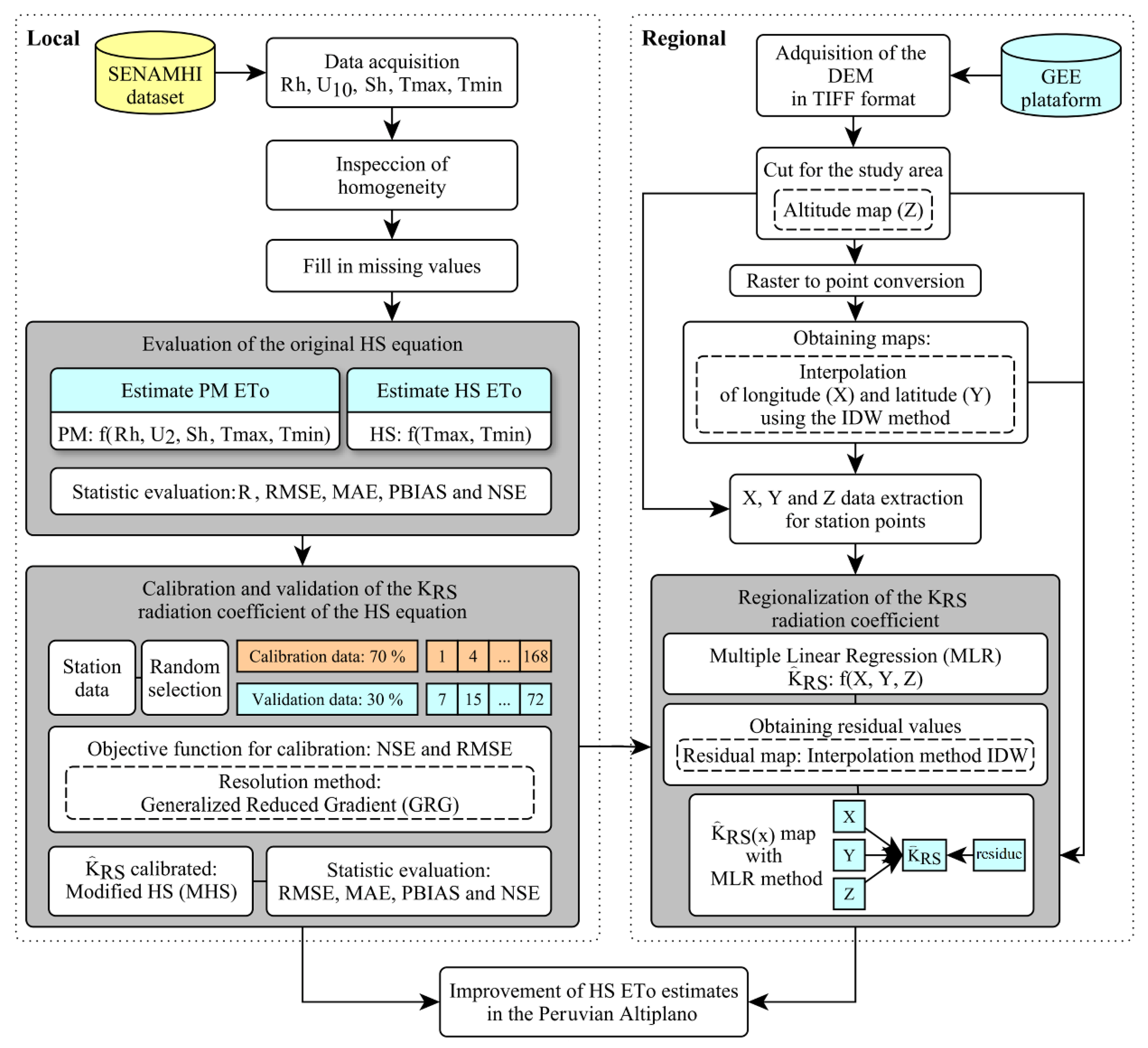
The flow diagram of Figure 3 summarizes the analysis procedure for the improvement of the Hargreaves–Samani reference evapotranspiration estimates.
3. Results and Discussion
3.1. Evaluation of the Original Hargreaves-Samani Equation
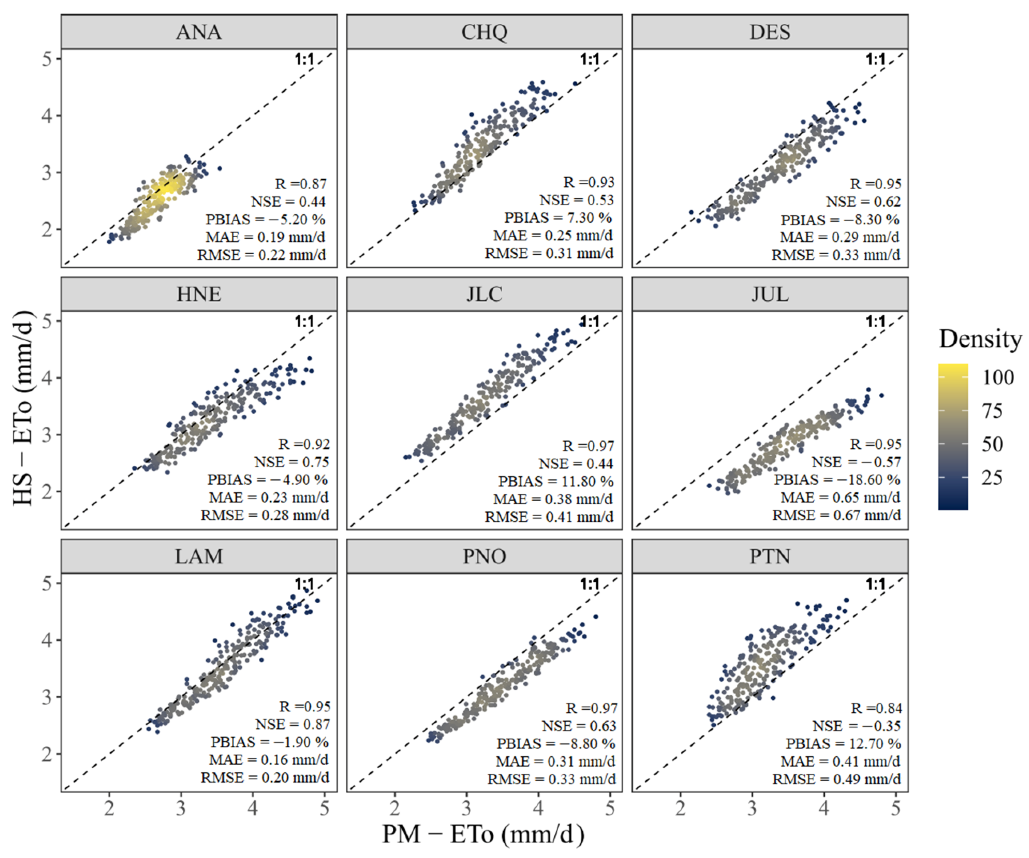
Figure 4 illustrates the comparison of ETo estimates by the original HS method versus the PM method. The value of KRS considered for the HS equation was 0.17 °C−0.5 for all weather stations. The precision of the ETo values of the original HS equation had significant variations in the SH-h and SH-d climatic zones identified in the study area (Table 1). The scatter diagrams reveal that the values of the correlation coefficient (R) within the two climatic zones oscillated between 0.84 and 0.97, presenting lower values in the ANA and PTN stations and higher values in the PNO and JLC stations. On the other hand, in relation to the values of the NSE vary between −0.57 and 0.87, NSE values lower than 0.50 were presented in the PTN, JUL, JLC and ANA stations, indicating poor performance. Meanwhile, values higher than 0.75 were presented in the of HNE and LAM stations, indicating very good performance according to the discretion of Moriasi et al. [43].
The PBIAS oscillates values between −18.60% and 12.70%, deducing that the HS equation tends to underestimate the ETo in the JUL, PNO, DES, ANA. HNE and LAM stations with values of −18.60%, −8.80%, −8.30%, −5.20%, −4.90% and −1.90%, respectively. On the other hand, it tends to overestimate the ETo in the PTN, JLC and CHQ stations whit values of 12.70%, 11.80%, and 7.30% respectively. The ETo underestimations occurred in the JUL, PNO, DES y HNE stations that are close to Lake Titicaca (LT), it was also observed in the LAM and ANA stations that are far from the LT, while the overestimations the ETo observed in the stations that are far from the LT. For the CHQ station that is in the SH-h climate classification, and the JLC and PTN stations with SH-d climate, the results are in accordance with that determined by Trajkovic [6], where the HS model generally overestimates the ETo in humid climate areas. However, the ANA and JUL station with the SH-h climate and DES, HNE, LAM and PNO stations with the SH-d climate, underestimated the ETo, therefore, the use of the HS equation is not very efficient.
Meanwhile, for Allen et al. [13], the HS equation tends to underestimate the ETo values under strong wind conditions and to overestimate the ETo under high relative humidity conditions. In this study, only the DES station reports a high wind speed, which tends to underestimate the ETo, while the other stations that registered lower wind speeds tended to underestimate and overestimate the ETo. On the other hand, in relation to relative humidity, the results do not agree with the ANA weather station, which tends to underestimate ETo.
On the other hand, the values of the MAE oscillate between 0.16 and 0.65 mm/d, presenting the lowest values in the LAM, ANA, HNE, CHQ and DES stations (0.16, 0.19, 0.23, 0.25 and 0.29 mm/d) and the high values in the PNO, JLC, PTN and JUL stations (0.31, 0.38, 0.41 and 0.65 mm/d). Likewise, the RMSE values vary between 0.20 and 0.67 mm/d, presenting low values occurred in the LAM, ANA, HNE, CHQ, DES and PUN stations (0, 20, 0.22, 0.28, 0.31, 0.33 and 0.33 mm/d) and high values in the JLC, PTN and JUL stations (0.41, 0.49 and 0.67 mm/d).
3.2. Calibration and Validation of the Radiation Coefficient KRS of the HS Equation
The results show that using a single value of KRS can lead to less precise estimates of ETo in the PA, thus, the calibrated values of the range from 0.150 °C−0.5 to 0.199 °C−0.5. For most of the stations, the values of differ from the coefficient suggested by Hargreaves and Samani [15], except that of the LAM station where a very close value was obtained ( = 0.173 °C−0.5). High values of were obtained at the DES, JUL, PNO and HNE stations close to LT, with values of 0.184 °C−0.5, 0.209 °C−0.5, 0.186 °C−0.5 and 0.179 °C−0.5, respectively, while low values were obtained at the CHQ, JLC and PTN stations with values of 0.158 °C−0.5, 0.152 °C−0.5 and 0.150 °C−0.5 respectively, which are the same ones that are far from the LT. The ANA station located at high altitude (4660 m.a.s.l.) and far from the LT registered a high value of = 0.179 °C−0.5. Ref. [30] showed that KRS values do not decrease with distance from the sea. At the same time, the standard values of 0.16 °C−0.5 and 0.19 °C−0.5 should not be assumed. In this regard, the precision of the ETo estimate improved for each weather station by adopting the calibrated and validated values in the HS equation.
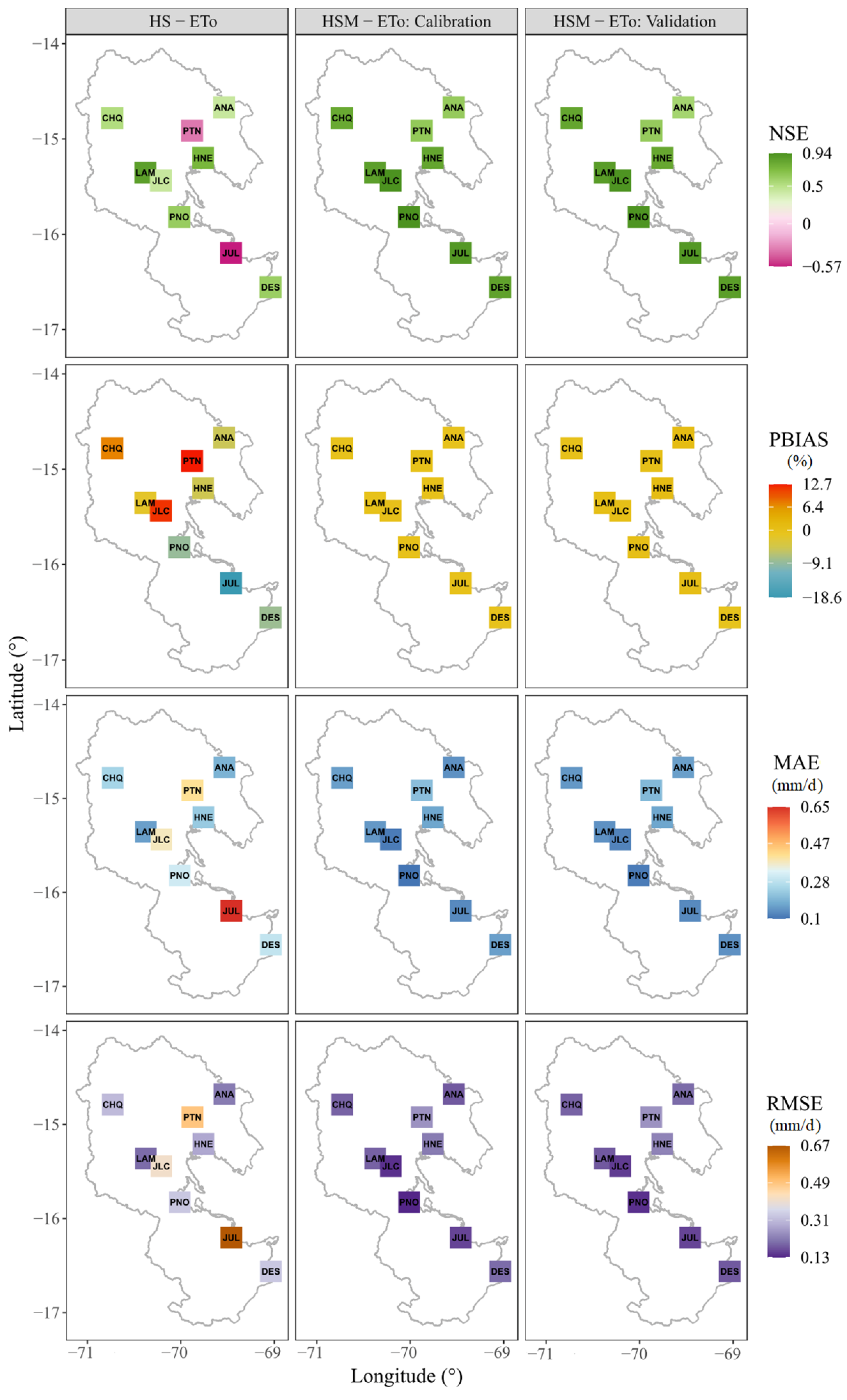
Figure 5 shows the spatial distribution of the NSE, PBIAS, MAE and RMSE of the ETo estimates from the HS and modified HS equation (HSM) for the nine stations. The performance indicators significantly improved the NSE values that oscillate between 0.64 and 0.94 for the calibration phase, while for the validation phase the NSE values oscillate between 0.58 to 0.93. The lowest values were presented in the ANA and PTN stations with 0.64 and 0.65 in the calibration phase, and values of 0.58 and 0.64 in the validation phase.
On the other hand, the PBIAS values oscillate between −0.52% and −0.01% in the calibration phase, presenting slight underestimations in all weather stations; however, in the validation phase the values oscillate between −0.58% and 1.34%, presenting underestimations in the CHQ and DES stations at −0.21% and −0.58% respectively, according to the discretion of Moriasi et al. [43] the PBIAS values are below ±5%, being considered ‘very good’.
Regarding the MAE, the HSM equation with calibrated and validated values presents low values for all weather stations, ranging between 0.02 and 0.00 mm/d, for the calibration phase. Meanwhile, for the validation phase, the MAE values oscillate between −0.02 and 0.05 mm/d, respectively. Likewise, for the calibration phase, the RMSE values are between 0.13 and 0.25 mm/d, while for the validation phase, the RSME values are between 0.14 and 0.25 mm/d. The precision indicators used agree with those found in studies conducted by Rodrigues and Braga [30], Paredes et al. [29] and Raziei and Pereira [5], where, after calibrating the value of the , the ETo led to very good results, being able to use the simplified equations (Table 3) for the estimation of the ETo locally.
3.3. Regionalisation of the Radiation Coefficient
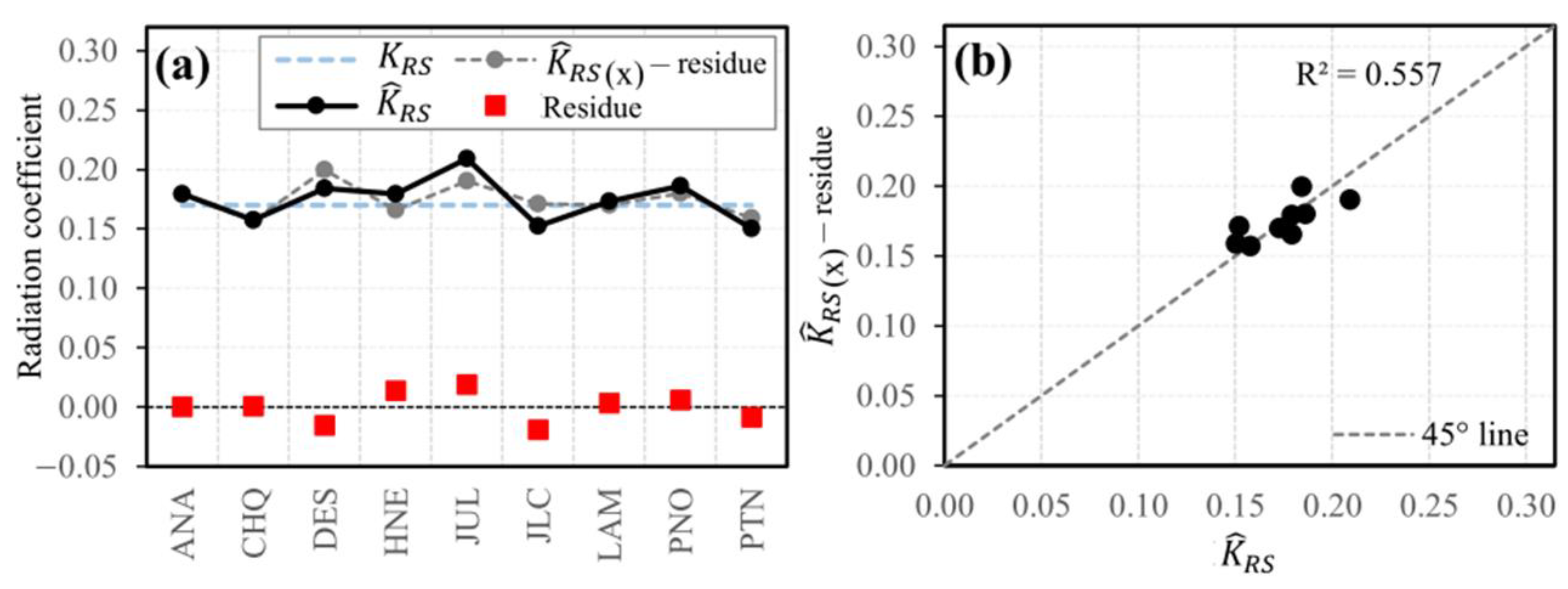
Considering the scarcity of climatic data, the regionalization of the for the PA is proposed. The RLM model was used to build the regionalization model of the based on geographic characteristics. The results of the correlation analysis between and the geographical characteristics of longitude, latitude and altitude resulted in a correlation equal to 0.59, −0.62 and 0.04 respectively. The latitude feature obtained the highest correlation compared with the longitude and altitude features. Consequently, the geographical characteristics (longitude, latitude and altitude) explained the variability of by 55.7% (R2 = 0.557) (Figure 6b). This study found that the regional equation of could better estimate ETo for regions with limited data within the PA, with the magnitude of R2 being acceptable for estimating in the PA from geographic characteristics.
The standard error for was 0.016. The confidence interval for the model parameter varies between −4.25303 and 3.70991, that for varies between −0.04514 and 0.04690, that for varies between −0.06647 and 0.01713 and that for varies between −0.00005 and 0.00012, with a confidence level of 95%. The residuals of for the station points, vary between −0.019 and 0.019 respectively (Figure 6a), being the applicable equation for the PA.
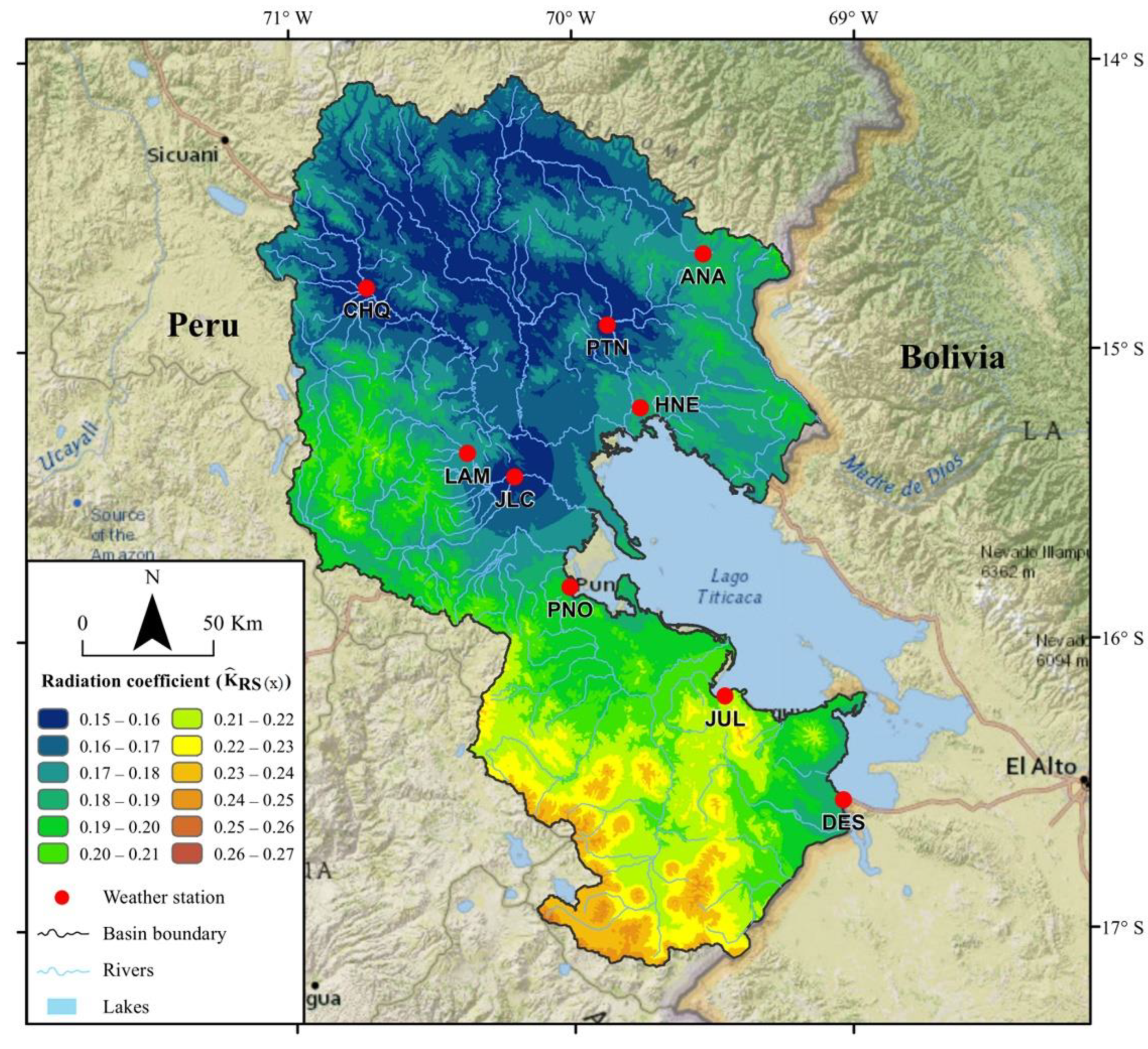
The values for the PA vary between 0.15 and 0.27. The spatial distribution is greater for the western, central and southern zone of the Altiplano, as it approaches the coastal areas; while lower values are observed for the northern zone there (Figure 7), these estimated values when regionalizing the radiation coefficient for the PA, are found in the range of the values reported by Samani [49] which oscillates between 0.12 and 0.24 °C−0.5, by Raziei and Pereira [5] obtained values that oscillate between 0.14 and 0.20 °C−0.5, while results obtained by Paredes et al. [50] show values that oscillate between 0.14 and 0.25 °C−0.5, respectively.
The regional equation to estimate the ETo in the PA based on the Hargreaves–Samani model is as follows:
where , is the predicted value at any point in the Peruvian Altiplano.
4. Conclusions
The main objective of the research was to improve the Hargreaves–Samani reference evapotranspiration estimates in the PA. The main conclusions are summarized below:
The HS model based on air temperature is recommended as the simplest and most practical method to estimate ETo. The ETo HS estimates were evaluated based on the ETo PM estimates in the PA. The period considered was from January 2000 to December 2019 on a monthly time scale. The ETo calculated with PM and HS showed a high correlation, but a great bias, with strong underestimations and overestimations of the ETo, requiring its local calibration before its use.
Due to its association of the radiation coefficient KRS with solar radiation, it is preferable to calibrate the values of KRS from the HS equation and thus obtain an HSM equation. The HSM model performed better than the HS model for each weather station. Better estimates of ETo were obtained with HSM after calibration of the radiation coefficient KRS of the HS equation, mainly removing biases.
The new values of the radiation coefficient of the HS empirical model for the PA are presented. The MLR model was used to regionalize the radiation coefficient KRS. The HS equation, together with the calibrated radiation coefficient KRS, can significantly improve the estimate of ETo over data-deficient regions within the PA.
It is important to note that although the MLR model used to regionalize the KRS has proven effective in estimating ETo in the study area, it is necessary to consider that the lack of availability of observed climatic data could affect its reliability in areas far from the meteorological stations used for calibration. Therefore, caution is recommended when using the HS equation with new KRS values in areas outside the study area and away from the meteorological stations, and further research is suggested to evaluate the applicability of the proposed approach in other regions with different climatic and topographic conditions. In this regard, future research lines could be explored, such as (1) examining the influence of other factors, such as soil moisture and vegetation cover, on the accuracy of ETo estimates using the HS model, (2) expanding the research to other regions with different climatic and topographic conditions to evaluate the applicability of the proposed methodology, and (3) exploring the regionalization of KRS based on additional climatic factors. These research lines could improve the accuracy of ETo estimates and, therefore, have a positive impact on the management and planning of water resources in different regions.
Author Contributions
Conceptualization, A.L., M.S.-D. and E.L.; methodology, A.L. and E.L.; formal analysis, E.L.; investigation, A.L. and E.L.; resources, A.L., M.S.-D. and E.L.; writing—original draft preparation, A.L. and E.L.; writing review and editing, A.L., M.S.-D. and E.L. All authors have read and agreed to the published version of the manuscript.
Funding
This research received no external funding.
Data Availability Statement
Not applicable.
Acknowledgments
Our thanks to the National Service of Meteorology and Hydrology (SENAMHI)—Peru for providing the meteorological information for carrying out this research study.
Conflicts of Interest
The authors declare no conflict of interest.
References
- Berti, A.; Tardivo, G.; Chiaudani, A.; Rech, F.; Borin, M. Assessing reference evapotranspiration by the Hargreaves method in north-eastern Italy. Agric. Water Manag. 2014, 140, 20–25. [Google Scholar] [CrossRef]
- Droogers, P.; Allen, R.G. Estimating reference evapotranspiration under inaccurate data conditions. Irrig. Drain. Syst. 2002, 16, 33–45. [Google Scholar] [CrossRef]
- Chipana, R.; Yujra, R.; Paredes, P.; Pereira, L.S. Determinación de la evapotranspiración de referencia con datos limitados en zonas de altura del Altiplano Boliviano aplicando la metodología de la FAO y la ecuación de Hargreaves-Samani. In I Congreso Boliviano de Riego y Drenaje; Facultad de Agronomía: La Paz, Argentina, 2010; pp. 12–14. [Google Scholar]
- Todorovic, M.; Karic, B.; Pereira, L.S. Reference Evapotranspiration estimate with limited weather data across a range of Mediterranean climates. J. Hydrol. 2013, 481, 166–176. [Google Scholar] [CrossRef] [Green Version]
- Raziei, T.; Pereira, L.S. Estimation of ETo with Hargreaves–Samani and FAO-PM temperature methods for a wide range of climates in Iran. Agric. Water Manag. 2013, 121, 1–18. [Google Scholar] [CrossRef]
- Trajkovic, S. Hargreaves versus Penman-Monteith under Humid Conditions. J. Irrig. Drain. Eng. 2007, 133, 38–42. [Google Scholar] [CrossRef]
- Muhammad, M.K.I.; Nashwan, M.S.; Shahid, S.; Ismail, T.B.; Song, Y.H.; Chung, E.S. Evaluation of empirical reference evapotranspiration models using compromise programming: A case study of Peninsular Malaysia. Sustainability 2019, 11, 4267. [Google Scholar] [CrossRef] [Green Version]
- Adamala, S.; Raghuwanshi, N.S.; Mishra, A.; Tiwari, M.K. Evapotranspiration modeling using second-order neural networks. J. Hydrol. Eng. 2014, 19, 1131–1140. [Google Scholar] [CrossRef]
- Srivastava, A.; Sahoo, B.; Raghuwanshi, N.S.; Singh, R. Evaluation of Variable-Infiltration Capacity Model and MODIS-Terra Satellite-Derived Grid-Scale Evapotranspiration Estimates in a River Basin with Tropical Monsoon-Type Climatology. J. Irrig. Drain. Eng. 2017, 143, 4017028. [Google Scholar] [CrossRef] [Green Version]
- Kumari, N.; Srivastava, A. An Approach for Estimation of Evapotranspiration by Standardizing Parsimonious Method. Agric. Res. 2020, 9, 301–309. [Google Scholar] [CrossRef]
- Hamed, M.M.; Khan, N.; Muhammad, M.K.I.; Shahid, S. Ranking of Empirical Evapotranspiration Models in Different Climate Zones of Pakistan. Land 2022, 11, 2168. [Google Scholar] [CrossRef]
- Pereira, L.S.; Allen, R.G.; Smith, M.; Raes, D. Crop evapotranspiration estimation with FAO56: Past and future. Agric. Water Manag. 2015, 147, 4–20. [Google Scholar] [CrossRef]
- Allen, R.G.; Pereira, L.S.; Raes, D.; Smith, M. Crop evapotranspiration: Guidelines for computing crop water requirements. FAO Irrigation and drainage paper 56. FAO Rome 1998, 300, D05109. [Google Scholar]
- Almorox, J.; Senatore, A.; Quej, V.H.; Mendicino, G. Worldwide assessment of the Penman–Monteith temperature approach for the estimation of monthly reference evapotranspiration. Theor. Appl. Climatol. 2018, 131, 693–703. [Google Scholar] [CrossRef]
- Hargreaves, G.H.; Samani, Z.A. Reference Crop Evapotranspiration from Temperature. Appl. Eng. Agric. 1985, 1, 96–99. [Google Scholar] [CrossRef]
- Almorox, J.; Grieser, J. Calibration of the Hargreaves–Samani method for the calculation of reference evapotranspiration in different Köppen climate classes. Hydrol. Res. 2016, 47, 521–531. [Google Scholar] [CrossRef] [Green Version]
- Bogawski, P.; Bednorz, E. Comparison and validation of selected evapotranspiration models for conditions in Poland (Central Europe). Water Resour. Manag. 2014, 28, 5021–5038. [Google Scholar] [CrossRef] [Green Version]
- Čadro, S.; Uzunović, M.; Žurovec, J.; Žurovec, O. Validation and calibration of various reference evapotranspiration alternative methods under the climate conditions of Bosnia and Herzegovina. Int. Soil Water Conserv. Res. 2017, 5, 309–324. [Google Scholar] [CrossRef]
- Awal, R.; Habibi, H.; Fares, A.; Deb, S. Estimating reference crop evapotranspiration under limited climate data in West Texas. J. Hydrol. Reg. Stud. 2020, 28, 100677. [Google Scholar] [CrossRef]
- Gavilán, P.; Lorite, I.J.; Tornero, S.; Berengena, J. Regional calibration of Hargreaves equation for estimating reference et in a semiarid environment. Agric. Water Manag. 2006, 81, 257–281. [Google Scholar] [CrossRef]
- Tabari, H.; Talaee, P.H. Local calibration of the Hargreaves and Priestley-Taylor equations for estimating reference evapotranspiration in arid and cold climates of Iran based on the Penman-Monteith model. J. Hydrol. Eng. 2011, 16, 837. [Google Scholar] [CrossRef]
- Mohawesh, O.E.; Talozi, S.A. Comparison of Hargreaves and FAO56 equations for estimating monthly evapotranspiration for semi-arid and arid environments. Arch. Agron. Soil Sci. 2012, 58, 321–334. [Google Scholar] [CrossRef]
- Pandey, V.; Pandey, P.K.; Mahanta, A.P. Calibration and performance verification of Hargreaves Samani equation in a humid region. Irrig. Drain. 2014, 63, 659–667. [Google Scholar] [CrossRef]
- Dorji, U.; Olesen, J.E.; Seidenkrantz, M.S. Water balance in the complex mountainous terrain of Bhutan and linkages to land use. J. Hydrol. Reg. Stud. 2016, 7, 55–68. [Google Scholar] [CrossRef] [Green Version]
- Cobaner, M.; Citakoğlu, H.; Haktanir, T.; Kisi, O. Modifying Hargreaves–Samani equation with meteorological variables for estimation of reference evapotranspiration in Turkey. Hydrol. Res. 2017, 48, 480–497. [Google Scholar] [CrossRef]
- Ravazzani, G.; Corbari, C.; Morella, S.; Gianoli, P.; Mancini, M. Modified Hargreaves-Samani equation for the assessment of reference evapotranspiration in Alpine river basins. J. Irrig. Drain. Eng. 2012, 138, 592–599. [Google Scholar] [CrossRef]
- Lavado Casimiro, W.S.; Lhomme, J.P.; Labat, D.; Guyot, J.L.; Boulet, G. Estimación de la evapotranspiración de referencia (FAO-56 Penman-Monteith) con limitados datos climáticos en la cuenca andina amazónica peruana. Rev. Peru. Geo Atmosférica 2015, 4, 31–43. [Google Scholar]
- Morales-Salinas, L.; Ortega-Farías, S.; Riveros-Burgos, C.; Neira-Román, J.; Carrasco-Benavides, M.; López-Olivari, R. Monthly calibration of Hargreaves–Samani equation using remote sensing and topoclimatology in central-southern Chile. Int. J. Remote Sens. 2017, 38, 7497–7513. [Google Scholar] [CrossRef]
- Paredes, P.; Fontes, J.C.; Azevedo, E.B.; Pereira, L.S. Daily reference crop evapotranspiration in the humid environments of Azores islands using reduced data sets: Accuracy of FAO-PM temperature and Hargreaves-Samani methods. Theor. Appl. Climatol. 2018, 134, 595–611. [Google Scholar] [CrossRef]
- Rodrigues, G.C.; Braga, R.P. Estimation of Reference Evapotranspiration during the Irrigation Season Using Nine Temperature-Based Methods in a Hot-Summer Mediterranean Climate. Agriculture 2021, 11, 124. [Google Scholar] [CrossRef]
- Servicio Nacional de Meteorología e Hidrología del Perú (SENAMHI). Climas del Perú—Mapa de Clasificación Climática Nacional; Dirección de Meteorología y Evaluación Ambiental Atmosférica: Lima, Perú, 2020. [Google Scholar]
- Huerta, A.; Lavado, W. ATLAS Zonas Áridas Del Perú: Una Evaluación Presente Y Futura; SENAMHI: Lima, Perú, 2021. [Google Scholar]
- Chen, J.; Chen, J.; Liao, A.; Cao, X.; Chen, L.; Chen, X.; He, C.; Han, G.; Peng, S.; Lu, M.; et al. Global land cover mapping at 30 m resolution: A POK-based operational approach. ISPRS J. Photogramm. Remote Sens. 2015, 103, 7–27. [Google Scholar] [CrossRef] [Green Version]
- Vera, L.; Villegas, E.; Oria, C.; Arboleda, F. Control de Calidad de Datos de Estaciones Meteorológicas E Hidrológicas Automáticas en El Centro de Procesamiento de Datos Del SENAMHI; Servicio Nacional de Meteorología e Hidrología del Perú (SENAMHI): Lima, Perú, 2021. [Google Scholar]
- Chiew, F.H.; Siriwardena, L. Trend/Change Detection Software. USER GUIDE; CRC for Catchment Hydrology: Clayton, Australia, 2005. [Google Scholar]
- Van Buuren, S.; Groothuis-Oudshoorn, K. Mice: Multivariate imputation by chained equations in R. J. Stat. Softw. 2011, 45, 1–67. [Google Scholar] [CrossRef] [Green Version]
- Tomas-Burguera, M.; Vicente-Serrano, S.M.; Beguería, S.; Reig, F.; Latorre, B. Reference 634 crop evapotranspiration database in Spain (1961–2014). Earth Syst. Sci. Data. 2019, 11, 1917–1930. [Google Scholar] [CrossRef] [Green Version]
- Woldesenbet, T.A.; Elagib, N.A.; Ribbe, L.; Heinrich, J. Gap filling and homogenization of climatological datasets in the headwater region of the Upper Blue Nile Basin, Ethiopia. Int. J. Climatol. 2017, 37, 2122–2140. [Google Scholar] [CrossRef]
- Jarvis, A.; Reuter, H.I.; Nelson, A.; Guevara, E. Hole-Filled SRTM for the Globe Version 4. Available from the CGIAR-CSI SRTM 90m Database. 2008. Available online: http://srtm.csi.cgiar.org (accessed on 15 July 2022).
- Ye, J.; Guo, A.; Sun, G. Statistical analysis of reference evapotranspiration on the Tibetan Plateau. J. Irrig. Drain. Eng. 2009, 135, 134–140. [Google Scholar] [CrossRef]
- Legates, D.R.; McCabe, G.J. Evaluating the use of ‘goodness-of-fifit’ measures in hydrologic and hydroclimatic model validation. Water Resour. Res. 1999, 35, 233–241. [Google Scholar] [CrossRef]
- Nash, J.E.; Sutcliffe, J.V. River flow forecasting through conceptual models part I—A discussion of principles. J. Hydrol. 1970, 10, 282–290. [Google Scholar] [CrossRef]
- Moriasi, D.; Arnold, J.; Van Liew, M.; Bingner, R.; Harmel, R.; Veith, T. Model evaluation guidelines for systematic quantifification of accuracy in watershed simulations. Trans. ASABE 2007, 50, 885–900. [Google Scholar] [CrossRef]
- Vu, T.T.; Li, L.; Jun, K.S. Evaluation of multi-satellite precipitation products for streamflow simulations: A case study for the Han River Basin in the Korean Peninsula, East Asia. Water 2018, 10, 642. [Google Scholar] [CrossRef] [Green Version]
- Moriasi, D.N.; Gitau, M.W.; Pai, N.; Daggupati, P. Hydrologic and water quality models: Performance measures and evaluation criteria. Trans. ASABE 2015, 58, 1763–1785. [Google Scholar]
- Willmott, C.J.; Matsuura, K. Advantages of the mean absolute error (MAE) over the root mean square error (RMSE) in assessing average model performance. Clim. Res. 2005, 30, 79–82. [Google Scholar] [CrossRef]
- Shiri, J.; Sadraddini, A.A.; Nazemi, A.H.; Marti, P.; Fard, A.F.; Kisi, O.; Landeras, G. Independent testing for assessing the calibration of the Hargreaves–Samani equation: New heuristic alternatives for Iran. Comput. Electron. Agric. 2015, 117, 70–80. [Google Scholar] [CrossRef]
- Feng, Y.; Jia, Y.; Cui, N.; Zhao, L.; Li, C.; Gong, D. Calibration of Hargreaves model for reference evapotranspiration estimation in Sichuan basin of southwest China. Agric. Water Manag. 2017, 181, 1–9. [Google Scholar] [CrossRef]
- Samani, Z. Discussion of “History and Evaluation of Hargreaves Evapotranspiration Equation ”by George H. Hargreaves and Richard G. Allen. J. Irrig. Drain. Eng. 2003, 130, 447. [Google Scholar] [CrossRef]
- Paredes, P.; Fontes, J.C.; Azevedo, E.B.; Pereira, L.S. Daily reference crop evapotranspiration with reduced data sets in the humid environments of Azores islands using estimates of actual vapor pressure, solar radiation, and wind speed. Theor. Appl. Climatol. 2018, 134, 1115–1133. [Google Scholar] [CrossRef]
Figure 1.
(a) Location of the study area and spatial distribution of weather stations and (b) land cover.
Figure 1.
(a) Location of the study area and spatial distribution of weather stations and (b) land cover.

Figure 2.
Variation of climatic factors as a function of latitude and altitude (a) P and ETo (b) Tmin and Tmax, (c) Rh and (d) Sh and U2.
Figure 2.
Variation of climatic factors as a function of latitude and altitude (a) P and ETo (b) Tmin and Tmax, (c) Rh and (d) Sh and U2.

Figure 3.
Flow diagram for the improvement of the Hargreaves–Samani reference evapotranspiration estimates in the PA.
Figure 3.
Flow diagram for the improvement of the Hargreaves–Samani reference evapotranspiration estimates in the PA.

Figure 4.
Scatter diagrams between values of ETo by the PM method versus original HS at the weather stations.
Figure 4.
Scatter diagrams between values of ETo by the PM method versus original HS at the weather stations.

Figure 5.
Spatial distribution of the NSE, PBIAS (%), MAE (mm/d) and RMSE (mm/d) from the ETo estimates of HS with original , HSM with in the calibration and validation phase. Study area in gray outline.
Figure 5.
Spatial distribution of the NSE, PBIAS (%), MAE (mm/d) and RMSE (mm/d) from the ETo estimates of HS with original , HSM with in the calibration and validation phase. Study area in gray outline.

Figure 6.
Regionalization of the calibrated radiation coefficient of the HS equation as a function of longitude, latitude and altitude: (a) variation of the original KRS, calibrated, and residuals; (b) scatterplot between and interpolated without addition of the residual.
Figure 6.
Regionalization of the calibrated radiation coefficient of the HS equation as a function of longitude, latitude and altitude: (a) variation of the original KRS, calibrated, and residuals; (b) scatterplot between and interpolated without addition of the residual.

Figure 7.
Spatial distribution of the radiation coefficient .


Table 1.
Coordinates of the weather stations used, average of the meteorological variables, aridity index and climatic classification.
Table 1.
Coordinates of the weather stations used, average of the meteorological variables, aridity index and climatic classification.
| Station | Lat. | Long. | Alt. | Tmax | Tmin | Rh | U2 | Sh | ETo | P | AI | CC |
|---|---|---|---|---|---|---|---|---|---|---|---|---|
| Ananea (ANA) | −14.676 | −69.534 | 4660 | 10.5 | −1.9 | 80.6 | 2.0 | 6.3 | 2.7 | 658.4 | 0.67 | SH-h |
| Lampa (LAM) | −15.361 | −70.374 | 3866 | 17.1 | −0.3 | 55.0 | 2.4 | 8.1 | 3.6 | 757.1 | 0.60 | SH-d |
| Chuquibambilla (CHQ) | −14.788 | −70.728 | 3918 | 16.3 | −2.2 | 61.3 | 2.1 | 7.2 | 3.2 | 787.0 | 0.67 | SH-h |
| Putina (PTN) | −14.921 | −69.876 | 3861 | 17.3 | 0.1 | 70.1 | 2.6 | 6.9 | 3.1 | 643.9 | 0.56 | SH-d |
| Huancané (HNE) | −15.207 | −69.758 | 3840 | 15.7 | 0.3 | 58.9 | 2.9 | 7.7 | 3.4 | 650.5 | 0.52 | SH-d |
| Juliaca (JLC) | −15.444 | −70.208 | 3838 | 17.8 | −0.5 | 75.0 | 1.5 | 7.8 | 3.2 | 624.9 | 0.53 | SH-d |
| Puno (PNO) | −15.826 | −70.012 | 3812 | 16.3 | 3.5 | 61.1 | 1.8 | 8.1 | 3.5 | 750.6 | 0.59 | SH-d |
| Juli (JUL) | −16.204 | −69.460 | 3830 | 14.1 | 3.0 | 58.3 | 2.4 | 8.4 | 3.5 | 948.3 | 0.78 | SH-h |
| Desaguadero (DES) | −16.563 | −69.037 | 3833 | 15.2 | 1.7 | 65.7 | 5.5 | 7.4 | 3.4 | 736.9 | 0.60 | SH-d |
Table 2.
List of statistical performance metrics used for the calibration and validation of the KRS of the HS equation for the estimation of ETo.
Table 2.
List of statistical performance metrics used for the calibration and validation of the KRS of the HS equation for the estimation of ETo.
| Statistical Performance | Equation 1 | Unit | Optimal Value |
|---|---|---|---|
| Correlation coefficient (R) | - | ±1 | |
| Nash–Sutcliffe efficiency (NSE) | - | 1 | |
| Percent bias (PBIAS) | % | 0 | |
| Mean absolute error (MAE) | mm | 0 | |
| Root mean square error (RMSE) | mm | 0 |
Notes: 1 Variables: is the estimated value with PM, is the calculated value, is the average of the estimated value with PM, is the average of the calculated value, and is the total number of data.
Table 3.
Modified HS equations for each weather station.
| Station | Recommended Equations |
|---|---|
| Ananea (ANA) | |
| Lampa (LAM) | |
| Chuquibambilla (CHQ) | |
| Putina (PTN) | |
| Huancané (HNE) | |
| Juliaca (JLC) | |
| Puno (PNO) | |
| Juli (JUL) | |
| Desaguadero (DES) |
Disclaimer/Publisher’s Note: The statements, opinions and data contained in all publications are solely those of the individual author(s) and contributor(s) and not of MDPI and/or the editor(s). MDPI and/or the editor(s) disclaim responsibility for any injury to people or property resulting from any ideas, methods, instructions or products referred to in the content. |
© 2023 by the authors. Licensee MDPI, Basel, Switzerland. This article is an open access article distributed under the terms and conditions of the Creative Commons Attribution (CC BY) license (https://creativecommons.org/licenses/by/4.0/).
Share and Cite
MDPI and ACS Style
Lujano, A.; Sanchez-Delgado, M.; Lujano, E. Improvement of Hargreaves–Samani Reference Evapotranspiration Estimates in the Peruvian Altiplano. Water 2023, 15, 1410. https://doi.org/10.3390/w15071410
AMA Style
Lujano A, Sanchez-Delgado M, Lujano E. Improvement of Hargreaves–Samani Reference Evapotranspiration Estimates in the Peruvian Altiplano. Water. 2023; 15(7):1410. https://doi.org/10.3390/w15071410
Chicago/Turabian StyleLujano, Apolinario, Miguel Sanchez-Delgado, and Efrain Lujano. 2023. "Improvement of Hargreaves–Samani Reference Evapotranspiration Estimates in the Peruvian Altiplano" Water 15, no. 7: 1410. https://doi.org/10.3390/w15071410
Note that from the first issue of 2016, this journal uses article numbers instead of page numbers. See further details here.