Changes in Tidal and Barometric Response of Groundwater during Earthquakes—A Review with Recommendations for Better Management of Groundwater Resources

Abstract

The effects of earthquakes on groundwater and aquifer properties can be quantified and monitored using water-level changes produced by tides and barometric pressure. Tidal and barometric responses are particularly useful in evaluating the impacts of unexpected events, such as earthquakes, because the signals are continuously generated and recorded over large areas of the Earth’s surface. The techniques for the extraction of tidal and barometric signals from the water-level time series are described in many excellent papers, here, we focus on reviewing the hydrogeologic interpretations of, and earthquake impacts on, these responses. We review how hydrogeology and earthquakes impact the groundwater response to Earth tides, and changes in barometric pressure and barometric tides. Next, we review the current understanding of the mechanisms responsible for earthquake-induced changes in aquifer confinement and permeability. We conclude with a summary of open questions and topics for future research, notably the value in long-term monitoring and analysis of the earthquake response at multiple tidal and barometric frequencies.

1. Introduction

Changes in the groundwater level in wells during earthquakes have been reported since antiquity, e.g., [1,2]. The analysis of such changes is important because it provides information on earthquake impacts on the flow and storage of groundwater. Most early studies focused on the occurrence of such responses, e.g., [3], their signs, duration, and spatial distribution, e.g., [3,4,5,6,7,8,9,10,11,12,13,14,15,16,17,18,19,20,21], their relation with the occurrence of liquefaction, e.g., [22,23] and mud volcanoes, e.g., [24], changes in groundwater level and streamflow e.g., [25,26,27,28], and their correlation with seismic energy and strain [29,30,31]. Analytical models for idealized aquifers were developed and used to simulate the co-seismic and post-seismic change in water levels, e.g., [12,32] and stream discharge, e.g., [14,26,33], with the general conclusion that the permeability of aquifers, especially their vertical permeability, may be enhanced by earthquakes [34,35,36]. A extensive review is provided by Wang and Manga [37].

The co-seismic change in aquifer permeability poses a challenge to the management of groundwater resources, which requires accurate knowledge of aquifer properties. These changes often cause confined aquifers to leak [38,39,40], which in turn may lead to the exchange of groundwater among different aquifers or between aquifers and the ground surface [38,41]. While most of these changes are reversible and the pre-seismic values are recovered after several weeks or months [42], some are long lasting, e.g., [43,44,45] and do not recover to the pre-seismic level for many years. In such cases, the management of groundwater resources based on the knowledge of the pre-seismic aquifer properties may lead to erroneous decisions. Because large earthquakes may occur unexpectedly and because aquifer leakage may cause hazardous waste to spread from repositories to groundwater resources, urgent action may sometimes be required. The tidal and barometric response methods reviewed in this paper make it possible for real-time, large-scale, and quantitative re-evaluation of the aquifer properties and the safety of groundwater resources after large earthquakes.

Here, we review recent advances in the study of earthquake impacts on groundwater systems based on analysis of the change in groundwater response to tides and barometric pressure. Quantitative evaluation of the earthquake effects on aquifer properties began with the application of analysis on the tidal and barometric pressure to this discipline, e.g., [42]. Because the response of groundwater to Earth tides is present in many groundwater records, this method has since been widely adopted in later studies of earthquake impacts on groundwater, e.g., [43,45,46,47,48,49,50,51,52,53,54,55,56]. Furthermore, large earthquakes, such as the 2008 M7.9 Wenchuan earthquake and the M9.0 Tohoku earthquake, have caused changes in the tidal response of groundwater across the Chinese mainland [49,57] and have offered the opportunity to investigate earthquake impacts on a regional scale.

Another naturally occurring change in the groundwater level in wells is caused by a change in the barometric pressure on the Earth’s surface, which induces changes in the pore pressure in aquifers and the water level in wells. The investigation of the hydraulic properties of both aquifers and aquitards based on the barometric response has been a topic of active research, e.g., [13,58,59]. A recent development is the joint application of the analysis of tidal and barometric responses to evaluate earthquake impacts on groundwater systems, which enables the study of hydrogeological changes over different frequencies and spatial scales [40,41,45,48,54,60,61,62].

We first review studies on earthquake impacts on groundwater systems using the interactions between Earth tides and groundwater. We then review studies on earthquake impacts on groundwater systems using the interaction between barometric pressure and groundwater. Some recent attempts to combine the different approaches were also reviewed. Finally, we suggest some directions for future research. We conclude this review with some recommendations for better management of groundwater resources, particularly in areas prone to natural or induced earthquakes and areas near the repositories of hazardous waste.

2. Groundwater Response to Earth Tides

2.1. Earth Tides

The gravitational attractions of the Sun and Moon deform the Earth (Figure 1a) and cause periodic volumetric strains in aquifers, which produce oscillations of pore pressure that, in turn, cause groundwater to flow between aquifers and wells (Figure 1b). Thus, the water level in wells oscillates, and the amplitude and phase depend on how pressure is transmitted in the subsurface.

Given that the ratio a/R is small, the lunar tidal potential on the Earth’s surface at a latitude $\alpha$ is approximately, e.g., [63]:

$$W_2=\frac{GM}{R}{\left(\frac{a}{R}\right)}^2\frac{3 {cos}^2\alpha -1}{2},$$

where $G$ is the gravitational constant, $M$ is the mass of the Moon, a is the Earth’s average radius, and R is the distance between the centers of the Earth and the Moon. This expression may be further decomposed into a diurnal term and a semi-diurnal term, e.g., [63]. Similar expressions may be derived for solar tides. In reality, the tidal potential is more complex because the Moon’s orbit about the Earth and the Earth’s orbit about the Sun are elliptical, the Moon’s orbital plane does not align with the Earth’s equator, nor is the Earth’s rotation aligned with the ecliptic plane. Hence, there are numerous components to Earth tides (

Table 1. Largest tides at a latitude of 50° (modified from [64] (p. 22)).

Darwin Name	Period (Day)	Frequency (cpd)	Origin	Vertical Displacement (mm)
Mm	27.554	0.0363	Moon	7
Mf	13.660	0.0732	Moon	14
Q1	1.1195	0.8933	Moon	19
O1	1.0758	0.9295	Moon	100
M1	1.0347	0.9665	Moon	8
P1	1.0027	0.9973	Sun	47
S1	1.0000	1.000	Sun	1
K1	0.9973	1.0027	Moon/Sun	141
J1	0.9624	1.0391	Moon	8
OO1	0.9294	1.0760	Moon	4
2N2	0.5377	1.8598	Moon	3
N2	0.5274	1.8961	Moon	21
M2	0.5175	1.9324	Moon	108
L2	0.5080	1.9685	Moon	21
S2	0.5000	2.0000	Sun	50
K2	0.4986	2.0056	Moon/Sun	14
M3	0.3450	2.8986	Moon	1

), but most are too small to be of concern for studies on the groundwater response to tides.

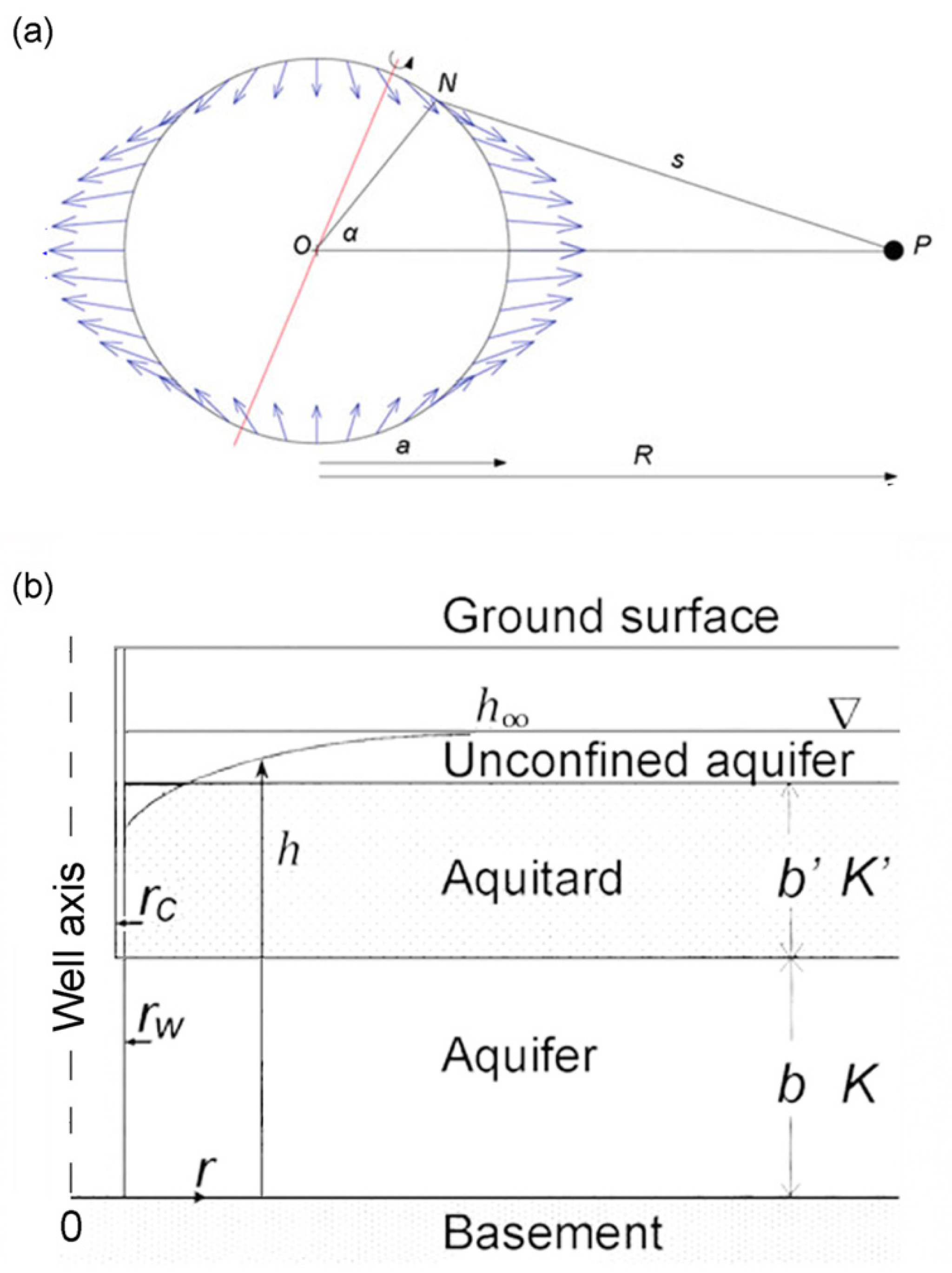
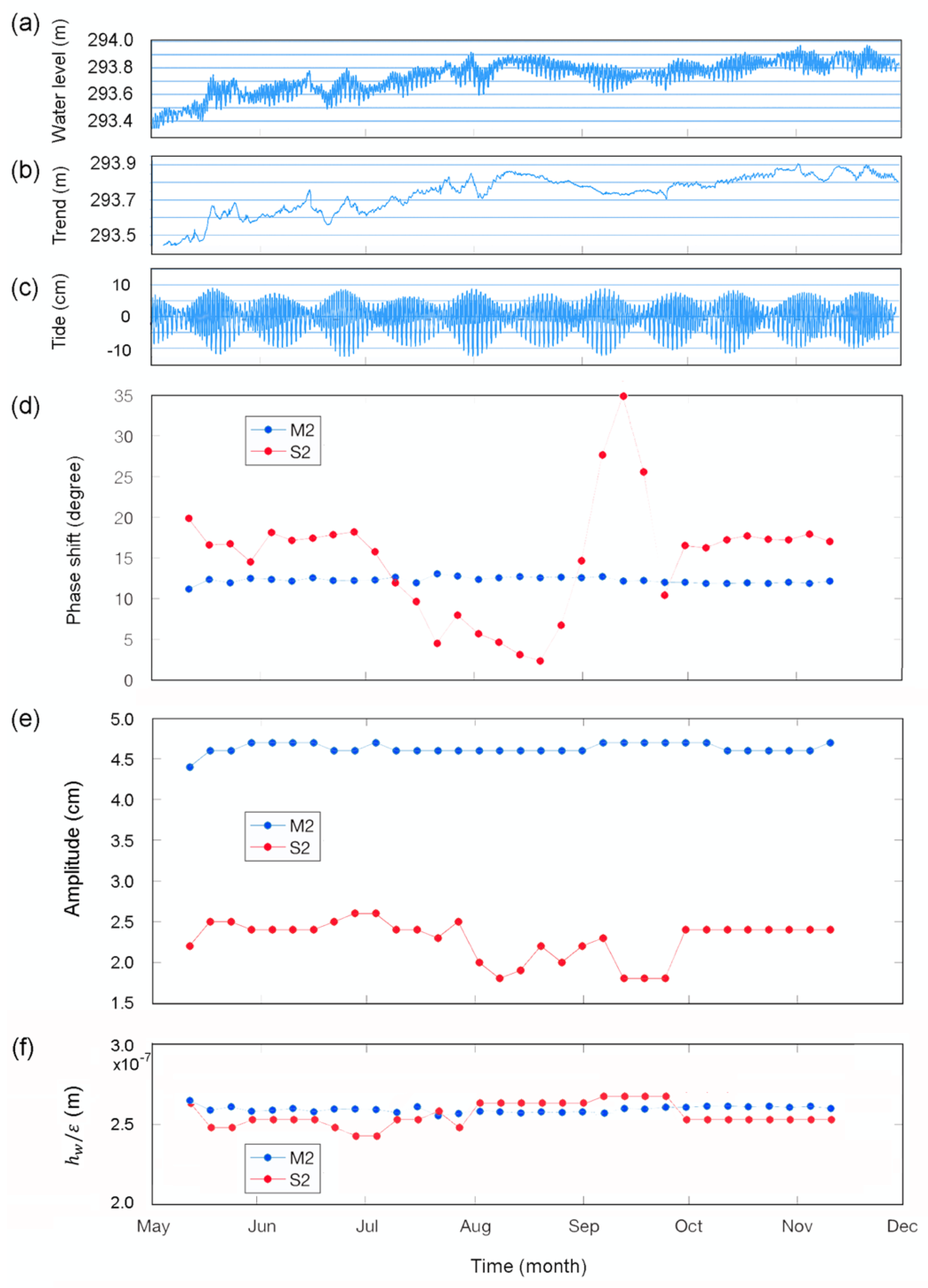
2.2. Tidal Response of Groundwater Level in Wells

Groundwater wells are the hydrogeologists’ scope to study groundwater systems. Hence, the analysis of changes in the water level in wells has been a time-honored study. Tidally-induced changes are often small in comparison to changes in water level (Figure 2), due to other causes such as seasonal recharge and groundwater extraction. Standard techniques are available for extracting tidal signals from water-level timeseries, such as using Fourier analysis, and readers are referred to some excellent reviews and tutorials on this aspect, e.g., [63,65]. Important for such analysis are long time series, high sampling frequency, and accurate measurements.

The flow of groundwater between the aquifer and the well causes changes in the phase and the amplitude of the water level in the well from those produced directly by the tidal strain. The difference in phase is known as the phase shift; a negative shift means that the response lags behind the tidal strain. The amplitude of the water-level response, if shown as the ratio between the observed amplitude and the amplitude of the tidal strain or the equivalent water level, is known as the amplitude ratio. Figure 2a shows the time series of the raw data for the groundwater level above the mean sea level from a USGS monitoring well (Figure 3) that opens to a carbonate aquifer (the Arbuckle) in NE Oklahoma at a depth of ~1 km below the surface. After the drift in the groundwater level was removed, the remaining time series shows the tidal signals (Figure 2c). Figure 2d shows the phase shift and amplitude of the response to the M₂ and S₂ tides in this time series, referenced to the local tidal volumetric strain; Figure 2f shows the ratio between the amplitudes of the water-level response and the volumetric tidal strain [38].

The phase shift and the amplitude of the M₂ tide are much more stable with time than those for the S₂ tide, which shows large fluctuations (Figure 2d,e) due to the changes in the thermal expansion of the atmosphere in response to solar heating (e.g., Figure 2d). As a consequence, the tides used most often for hydrological studies are the semi-diurnal and the diurnal lunar tides that are denoted as the M₂ and O₁ tides, respectively.

Direct measurement of the tidal strain is not available in most wells, and a theoretical tidal strain is often calculated at the well location and used as the reference for the observed tidal response. This procedure introduces some uncertainty into the response analysis because tidal strain is known to be affected by the local geology, topography, and underground cavities [66,67], which are difficult to correct. Locations close to coasts can also be affected by ocean tides.

2.3. Interpretation of Tidal Response of Groundwater in Aquifers

To interpret the tidal response data, hydrogeological models for the flow of groundwater between the well and the aquifer are needed. Two classical models have most often been invoked to interpret the observed tidal response. The model used for interpreting the tidal response with a negative phase shift is the confined aquifer model [63,68]. The model used for interpreting the tidal response with a positive phase shift is the unconfined aquifer model [11,63,69]. Reviews of these models are given by McMillan et al. [70] and Cutillo and Bredehoeft [71]. Most aquifers, however, are neither perfectly confined nor perfectly unconfined, e.g., [72], because the permeability of an aquitard cannot be zero, but is finite at time scales above a threshold. The interpretation of the tidal response of groundwater in such aquifers requires a model for leaky aquifers [38].

The well that provided the data shown in Figure 2 is located in northeastern Oklahoma (Figure 3a) and opens at a depth of ~900 m to a carbonate aquifer (the Arbuckle aquifer, Figure 3b) that has long been considered confined and used as a repository for the injection of wastewater co-produced from hydrocarbon exploration. Figure 3b shows a simplified diagram for the major geologic units intersected by the USGS Oklahoma deep well. It shows that the Arbuckle aquifer lies on the top of a crystalline basement and is overlain by an aquitard consisting of a sequence of layered rocks with a basal shale. The aquitard is in turn overlain by a layer of unconsolidated sediments. Given the layered structure of the aquitard (Figure 3b), its average vertical conductivity may be estimated by the harmonic mean of permeability of the layers, which is dominated by the layer with the lowest permeability, e.g., [73], in this case the basal shale (Figure 3b). In other words, according to this estimate, the value of K′ for the layered aquitard may be expected to be close to that of the basal shale [38], consistent with the suggestion that the aquifer is confined. However, the groundwater response to the M₂ tide in the USGS well shows a positive phase (Figure 2d) that characterizes an unconfined model, according to the traditional interpretation. Hence, neither the confined aquifer model nor the unconfined aquifer model may completely satisfy the observational data. The need to explain this apparent contradiction is important because of the large increase in induced earthquakes in the mid-continental U.S. produced by fluid injection, as exemplified by the occurrence of three large ($M\ge 5$) earthquakes in Oklahoma in 2016 (Figure 3a).

To explain the positive phase shift for an aquifer bounded by low-permeability formations, Wang et al. [38] derived a model for a semi-confined aquifer. The model may be reduced to that for a confining aquifer when the leakage becomes very small; it also provides predictions similar to that of an unconfined aquifer when the leakage becomes very large [38]. The semi-confined aquifer model is, therefore, a versatile model and is described below to illustrate how the analysis of tidal response of groundwater may be applied to assess the impact of earthquakes.

Assuming that the aquifer is laterally extensive and the leakage through the aquitard is vertical [74], the model of the tidally-induced groundwater flow may be described as [38]:

$$T\left[\frac{{\partial }^{2}h}{{\partial r}^2}+\frac{1}{r}\frac{\partial h}{\partial r}\right]-\frac{K^{\prime }}{b^{\prime }}h=S\frac{\partial h}{\partial t}-\frac{SB{K}_u}{\rho g}\frac{\partial \epsilon }{\partial t}$$

(1)

where $h$ is the hydraulic head in the aquifer, r is the radial distance from the studied well, T and S are the transmissivity and storativity of the aquifer, respectively, and are related to the hydraulic conductivity K and the specific storage S_s of the aquifer of T = bK and S = bS_s, $\epsilon$ is the tidally-induced oscillating volumetric strain of the aquifer, B is the Skempton’s coefficient, $K_u$ is the undrained bulk modulus, and K′ and b′ are the vertical hydraulic conductivity and the thickness of the aquitard, respectively. The hydraulic conductivity is generally a second rank tensor and is related to the permeability tensor as follows:

$$K=\frac{{\rho }_f gk}{\mu }.$$

(2)

where ${\rho }_f$ and µ, respectively, are the density and viscosity of the pore water, and $g$ is the gravitational acceleration. In most groundwater studies, aquifers and aquitards are assumed to be isotropic and the tensor notations are replaced by K and k. Furthermore, since the density and viscosity of groundwater are usually nearly constant, it may be more convenient to use K instead of k under common conditions.

In this semi-confined aquifer model, the unconfined aquifer is taken to be part of the aquitard with atmospheric pressure on its upper boundary. Moreover, it is assumed in this model that the storage of the aquitard is negligible. The boundary conditions for our problem are:

$$h (r,t)=h_{\infty }\left(t\right) \mathrm{at} r=\infty ,$$

(3)

$$h \left(r,t\right)=h_w\left(t\right) \mathrm{at} r=r_w, \mathrm{and}$$

(4)

$$-2\pi r_{w}T{\left(\partial h/\partial r\right)}_{r=r_w}=\pi {r_c}^2\left(\partial h_w/\partial t\right)=-i\omega h_w\pi {r_c}^2 \mathrm{at} r=r_w$$

(5)

where:

$$h_w=h_{wo}{e}^{i\omega t}$$

(6)

is the oscillating water level in the well with an amplitude (complex) of $h_{wo}$ and a frequency of $\omega$, r_w is the radius of the screened portion of the well, and r_c is the inner radius of the well casing in which the water level moves up and down.

The procedure for solving the boundary value problem follows previous works on confined aquifers [68] and is given in [38]. Assuming $\epsilon ={\epsilon }_o{e}^{i\omega t}$, where ${\epsilon }_o$ is the (complex) amplitude of the tidally-induced strain, the solution to (1) with boundary conditions (3) to (5) is:

$$h_{w,o}=\frac{1}{\xi }\frac{i\omega S}{\left(i\omega S+K^{\prime }/b^{\prime }\right)}\left(\frac{B{K}_u{\epsilon }_o}{\rho g}\right),$$

(7)

$$\xi =1+{\left(\frac{r_c}{r_w}\right)}^2\frac{i\omega r_w}{2T\beta }\frac{K_o\left(\beta r_w\right)}{K_1\left(\beta r_w\right)},$$

(8)

$$\beta ={\left(\frac{K^{\prime }}{T{b}^{\prime }}+\frac{i\omega S}{T}\right)}^{1/2},$$

(9)

where $K_o$ and $K_1$ are the modified Bessel functions of the second kind and of the zeroth and first orders, respectively. The amplitude ratio and the phase shift of the tidal response are, respectively,

$$A=\left|h_{w,o}/\left(\frac{B{K}_u{\epsilon }_o}{\rho g}\right)\right|,$$

(10)

$$\eta =\arg \left[h_{w,o}/\left(\frac{B{K}_u{\epsilon }_o}{\rho g}\right)\right].$$

(11)

Expressions (10) and (11) relate the amplitude ratio and the phase shift of the tidal response of the groundwater to three important parameters of the groundwater system, i.e., the vertical hydraulic permeability K′ of the leaky aquitard, the horizontal transmissivity T, and the storativity S of the aquifer. Given the amplitudes and phases of the observed M₂ and O₁ tides, the above expressions may be used to invert for the hydraulic parameters of the groundwater system. For the USGS Oklahoma deep well that opens to the Arbuckle aquifer (Figure 2), independent measurements exist for T and S [38]. Using these parameters together with the response of the groundwater in the USGS Oklahoma deep well to the M₂ tide, Wang et al. [38] estimated K′ ~3 × 10⁻⁸ to 3 × 10⁻⁷ m/s for the average vertical conductivity of the aquitard above the Arbuckle, which is many orders of magnitude greater than that estimated for an assumed intact aquitard [38]. This huge discrepancy between the permeability estimated from the observed tidal response and that for an assumed intact aquitard suggests that the aquitard near the well may have been breached by subvertical fractures. This suggestion was further supported by independent measurements of the electrical conductivity of the groundwater in the USGS Oklahoma deep well [41].

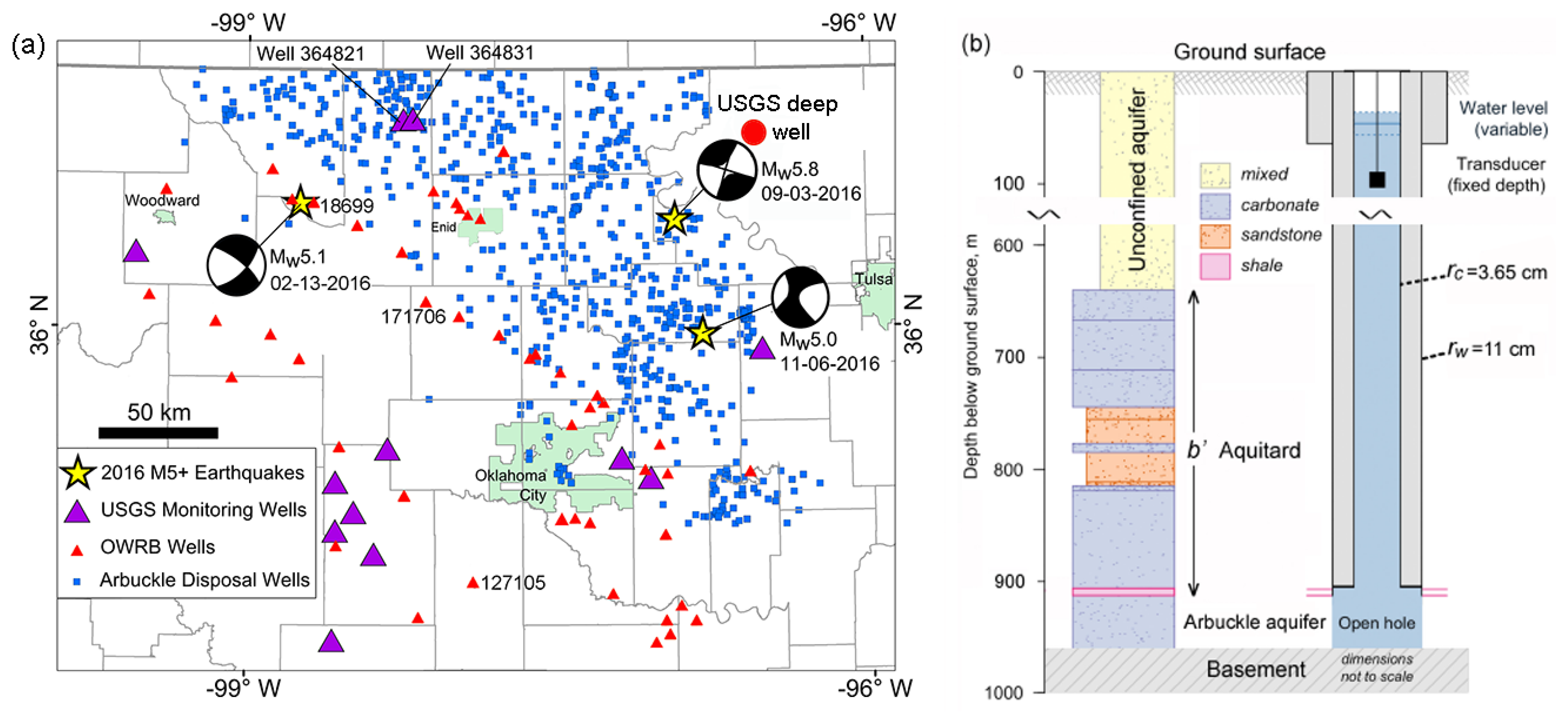
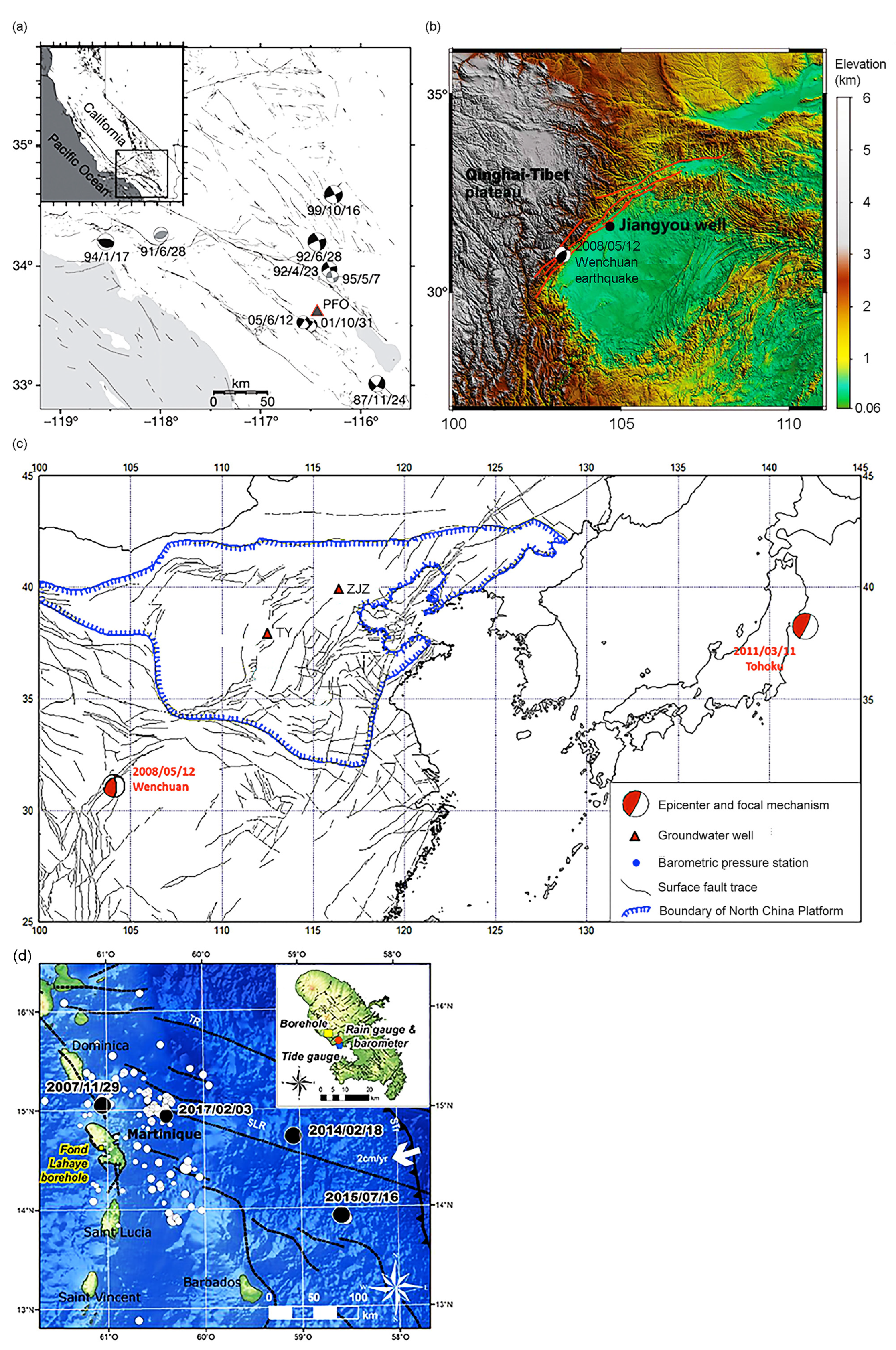
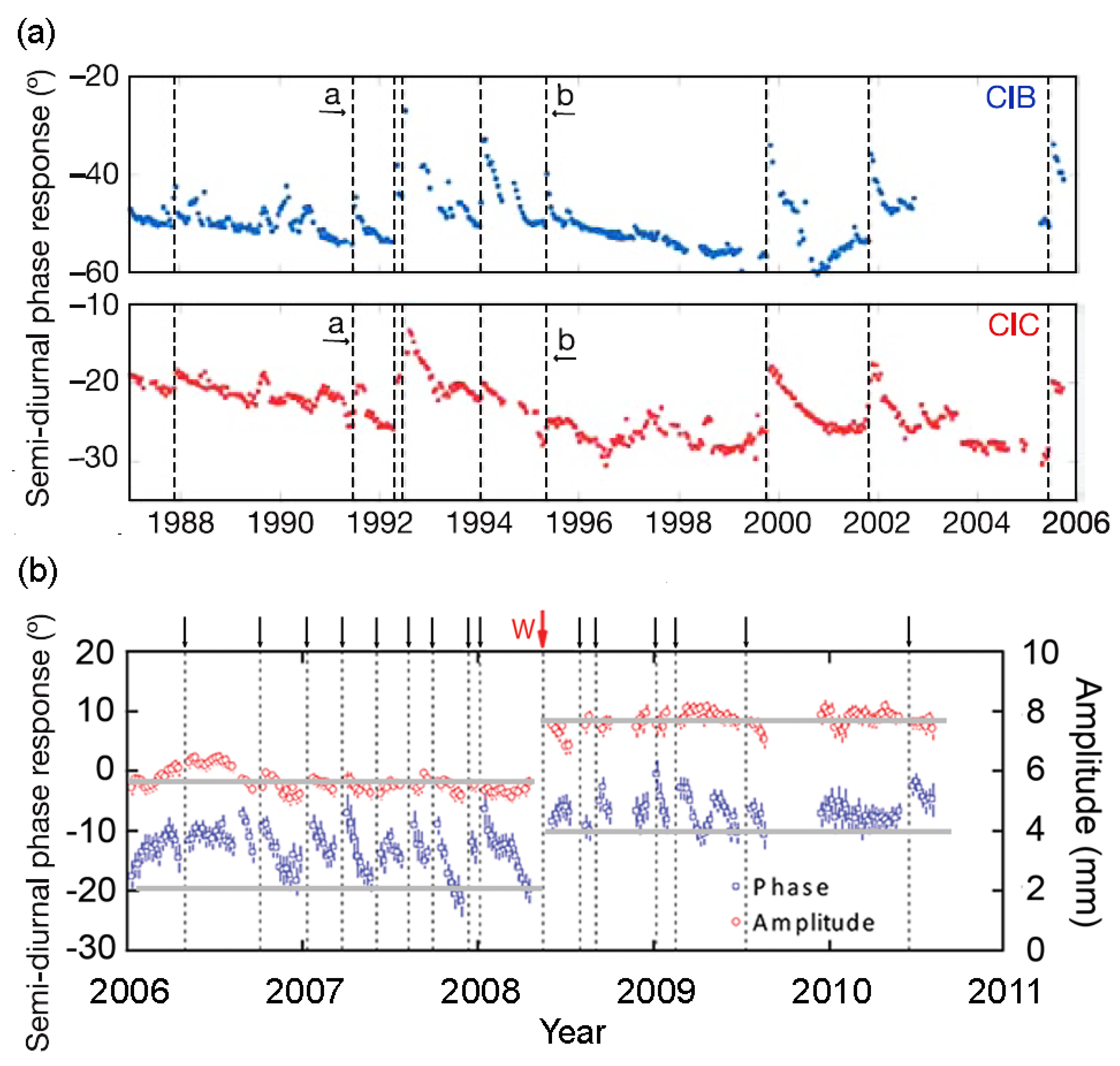
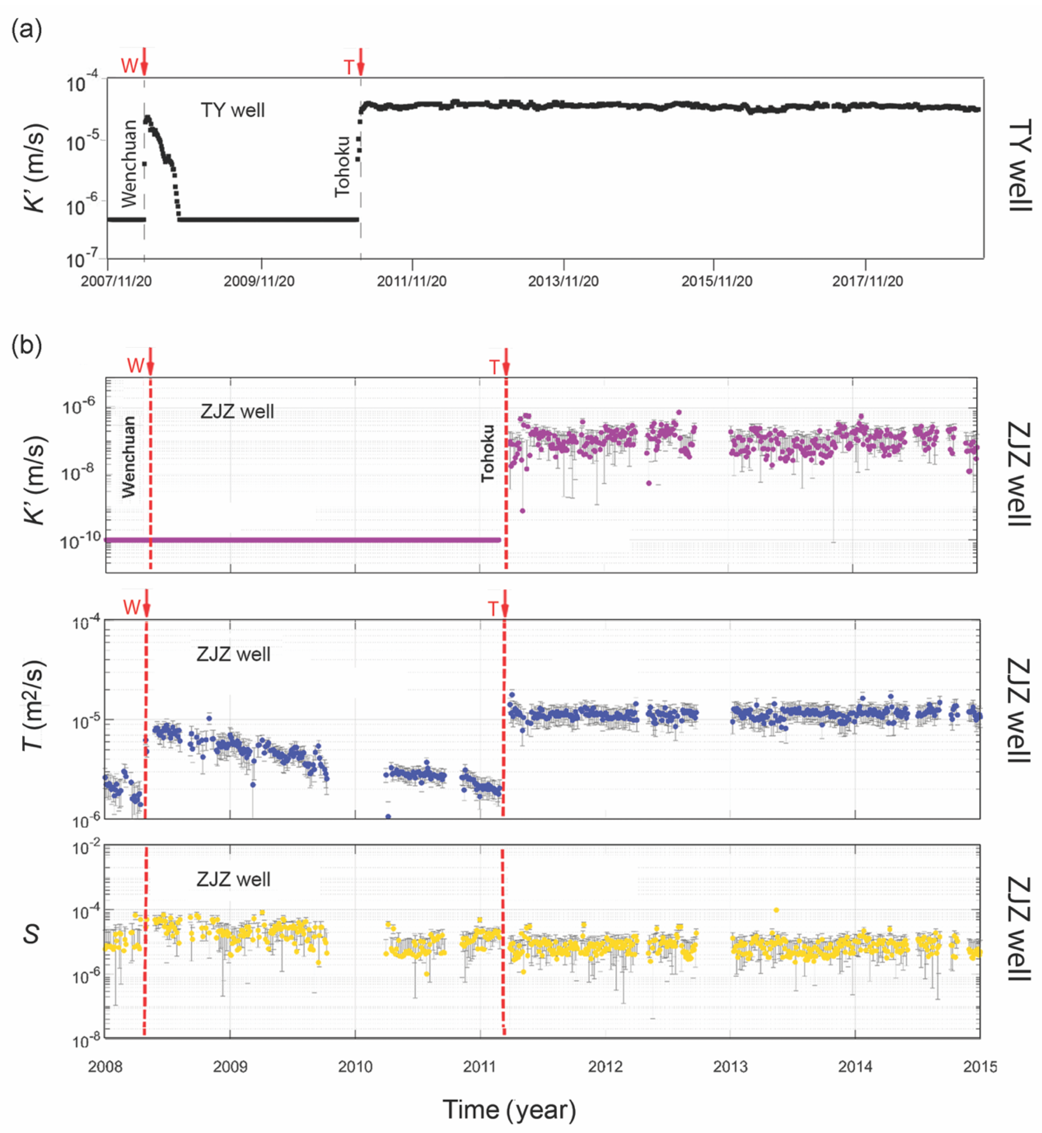
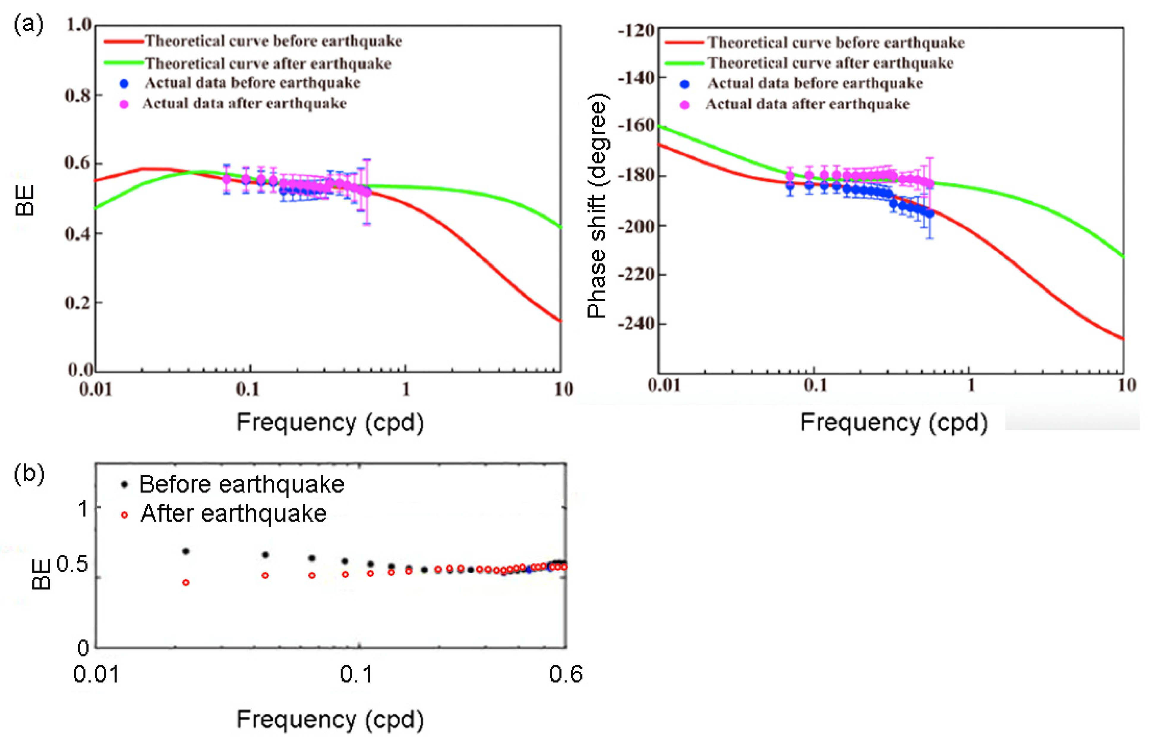
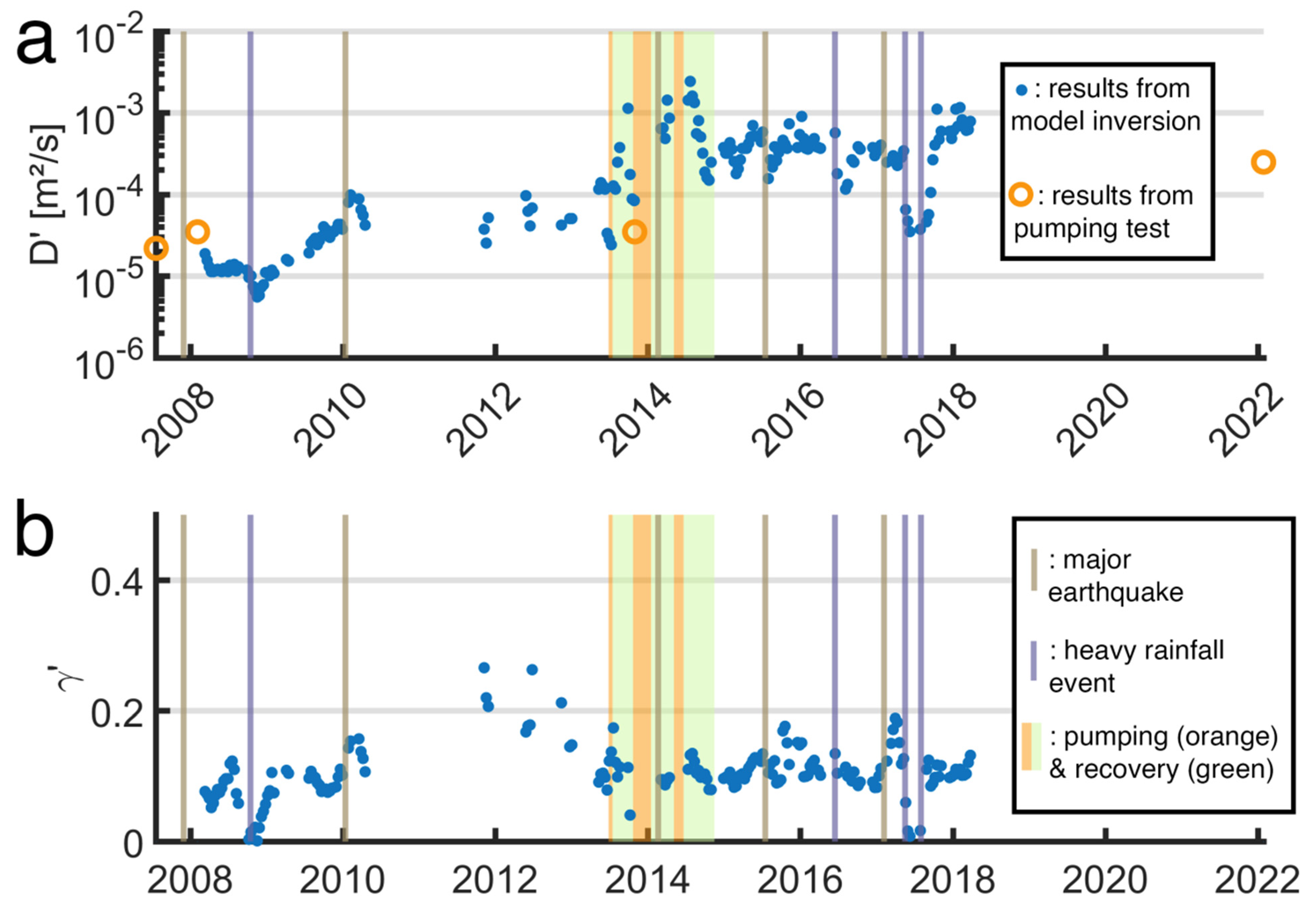
2.4. Assessing Earthquake Impact on Groundwater from Its Response to Earth Tides

Using the groundwater response to Earth tides in two wells in southern California (Figure 4a), Elkhoury et al. [42] found transient and recoverable changes in the water levels during and after earthquakes (Figure 5a). The wells open to a fractured aquifer in the granitic basement and the co-seismic water-level responses were interpreted with the confined aquifer model [68] to identify transient and reversible changes to the aquifer permeability. Liao et al. [43], on the other hand, found a tidal response after the 2008 M7.9 Wenchuan earthquake in the JY (Jiangyou) well in Sichuan (Figure 4b), China, which did not recover, but stayed at the co-seismic level for many years afterwards (red arrow in the top row of Figure 5b), even though the tidal responses of the groundwater in the same well to many smaller earthquakes (black arrows in Figure 5b), both before and after the Wenchuan earthquake, were transient and reversible, similar to the observations reported in [42]. The distinct difference between the change in the tidal response during the Wenchuan earthquake and the other earthquakes, suggests that distinctly different mechanisms were at play [44]. This well is only ~20 km from the ruptured fault of the 2008 M7.9 Wenchuan earthquake; the closeness of the well to the ruptured fault may be partly responsible for the distinct change in the tidal response during and after this earthquake. The coordinates and depths of these wells, the lithology of the aquifers, and their epicentral distances to some earthquakes are listed in

Table 2. Well locations, well depths, lithology of the aquifers, and epicentral distances to some earthquakes reviewed in this paper.

Well Names	Locations	Well Depth (m)	Aquifer Lithology	Aquitard Lithology	Epicentral Distance (km)
					Wenchuan Earthquake	Tohoku Earthquake
USGS Oklahoma deep well	36.73 N, 96.53 W	960	Carbonates	Shale, sandstone, carbonates	(Not studied)	(Not studied)
Piñor Flat Observatory 1	33.61 N, 116.46 W	211 (CIB) 137 (CIC)	Fractured granodiorite	Unfractured granodiorite	(Not studied)	(Not studied)
JY 2 (Jiangyou)	31.82 N, 104.76 E,	4000	Sandstone	Shale	21 km from ruptured fault	3480
ZJZ 3 (Zuojiazhuang)	39.95 N, 116.45 E	2600	Dolomite	Shale, mudstone	1532	2260
TY 4 (Taiyuan)	37.72 N, 112.43 E	765	Limestone dolomite	Marlstone	1115	2614
Fond Lahaye borehole 5	~14.6 N ~61.1 W	62	Fractured andesite	Altered andesite	(Not studied)	(Not studied)

Notes: ¹ Elkhoury et al. [42]; ² Liao et al. [43]; ³ Zhang et al. [45]; ⁴ Shi et al. [17]; ⁵ Thomas et al. [60].

.

Most interpretations of the tidal response of groundwater to earthquakes, such as those shown in Figure 5, were based on either the confined aquifer model [63,68] (or the unconfined aquifer model [13,63,69]. Given the ability of the semi-confined aquifer model [38] to estimate the vertical conductivity of aquitards, it has been increasingly used to interpret the groundwater response to Earth tides and study the effects of earthquakes, e.g., [17,45,75].

After the 2011 M9.1 Tohoku earthquake in Japan, some wells in China (Table 1), more than 2000 km away from the epicenter, also showed irreversible changes in the tidal response (Figure 4c,d; [45,51,75]). The upper two rows of Figure 6a show the phase shift and amplitude ratio of the groundwater response to the M₂ tide in the Taiyuan (TY) well in central China [51]; the phase shift increased but the amplitude ratio decreased both during the 2008 Wenchuan earthquake (red arrow marked W) and during the 2011 Tohoku earthquake (red arrow marked T). The changes during the Tohoku earthquake stayed at the co-seismic level for many years, but those during the Wenchuan earthquake were transient and quickly recovered to the pre-seismic level.

During the same earthquake, a well in northern China, the Zuojiazhuang (ZJZ) well (Figure 4c), showed a different response. This is a deep (2600 m) well, screened between depths of 2079 and 2600 m and is open to an aquifer of late Precambrian carbonate rocks. The aquifer is overlain by an aquitard of younger volcanic rocks and breccia, tuff, sandstone, and mudstone more than 2 km thick. Zhang-Shi et al. [39] analyzed the tidal response of the water level to the M₂ tide in this well and found large co-seismic increases in both the phase shift, from −40° to ~2°, and in the amplitude ratio, from 2 to 3 m/microstrain, during the Tohoku earthquake. Zhang-Wang et al. [45] re-analyzed the water-level response in the same well to both the M₂ and the O₁ tides. They found that the phase shift and amplitude ratio of the M₂ and the O₁ tides both increased in the ZJZ well during the Tohoku earthquake and remained at the co-seismic level for many years afterwards (Figure 6b). After the Wenchuan earthquake (red arrow marked W), on the other hand, the co-seismic increases of the phase shift and the amplitude ratio recovered gradually to the pre-seismic level.

Applying the semi-confined model to the groundwater response to the M₂ tide in the TY well, Shi et al. [51] interpreted the co-seismic change in the tidal response in the TY well as corresponding to the co-seismic increase in the vertical conductivity of the aquitard that recovered afterwards to the pre-seismic level (Figure 7a). During the Tohoku earthquake, the vertical conductivity increased from ~5 × 10⁻⁷ m/s to 5 × 10⁻⁵ m/s, but the increase stayed at the co-seismic level for many years (Figure 7a). Zhang et al. [45] employed the same model for the semi-confined aquifer and carried out an inversion for the unknown K′ of the aquitard, and T and S for the aquifer, from the responses to both the M₂ and O₁ tides in the ZJZ well, using the nonlinear least-square inversion. A lower limit of 10⁻¹⁰ m/s was set for K′ in the inversion to prevent the occurrence of singularity. The results of the inversion (Figure 6b; Zhang et al. [45]) showed that K′ stayed at the set minimum of 10⁻¹⁰ m/s from 2007 to 2011 before the Tohoku earthquake, suggesting that the aquifer was well confined before the Tohoku earthquake; however, during the Tohoku earthquake, K′ increased by three orders of magnitude from 10⁻¹⁰ m/s to 10⁻⁷ m/s, showing that the confinement of the aquifer was breached by the earthquake. T also increased from ~2 × 10⁻⁶ to ~2 × 10⁻⁵ m²/s during the earthquake. Furthermore, both these increases stayed at the co-seismic level for many years until the end of the study (Figure 6b; [45]). During the Wenchuan earthquake, no change in K′ was revealed, but T increased from ~2 × 10⁻⁶ to ~9 × 10⁻⁶ m/s and recovered gradually afterwards. Errors in the inverted S were too large to clearly identify the co-seismic changes.

One challenge to interpreting tidal responses is that different conceptual models may be able to explain the same observations. For example, Zhang et al. [55] reassessed the tidal responses from the well ZJZ (Figure 6b) assuming that the water-level changes were caused by volumetric changes in the transmissive fractures that intersect the well. Pressure changes in a fracture depend on the orientation of the fracture relative to the principal directions of the changing tidal strain and, thus, the amplitude and phase of the water-level changes will depend on the fracture orientation. In this model, both phase leads and lags are possible. Using the model of Hanson and Owen [76] and the amplitude and phase of the water-level response to the O₁ and M₂ tides, Zhang et al. [55] proposed that the apparent orientation of the fractures changed after the earthquakes. The underlying assumption behind the fracture orientation model is that the well is recording strain in the fracture and that hydraulic flows (and hence finite permeability) can be neglected. Since new fractures with different orientations are not likely to be created by the small stresses from these earthquakes, Zhang et al. [55] suggested that the connections between the pre-existing fractures were unlogged leading to changes in the apparent fracture orientation. The difference in the interpretations is non-trivial: Zhang et al. [45] inferred that the deep aquifers became much less well confined, whereas Zhang et al. [55] inferred changes in the apparent orientation of the fractures. Both models, however, do require a change in the hydrogeological properties of the aquifers and pathways for fluid flow.

Another challenge in the interpretation of tidal responses arises from the structures in the aquifers. For example, Zhang et al. [56] showed that fine layers of shale, which commonly occur in thick sandstone aquifers, introduce anisotropy to the aquifer, which may significantly affect the predicted phase shift in the tidal response and, thus, impact the interpretation of the observation. Another fine structure that may affect the tidal response of groundwater is the boundary between the layers of different permeabilities and grain sizes. Using ten years of continuous groundwater data from a well in southwest China, Liao et al. [77] showed that the groundwater in an unconfined aquifer changed its tidal response from being confined-like to being unconfined-like when the water level rose across the boundary between a fine-grained layer and a coarse-grained layer above. The authors explained this transition as due to the appearance of a confining capillary zone when the water table is below the upper boundary of the fine-grained layer, and its disappearance when the water level rises above this boundary. Even though the water-level rise in this study was due to seasonal precipitation, the same change in the tidal response may be expected if the water-level rise is earthquake induced. The introduction of fine structures into a model may make the model more realistic but, at the same time, it increases the number of unknown parameters and makes the inversion of the parameters from the observations under constrained. This point will be discussed further in a later section.

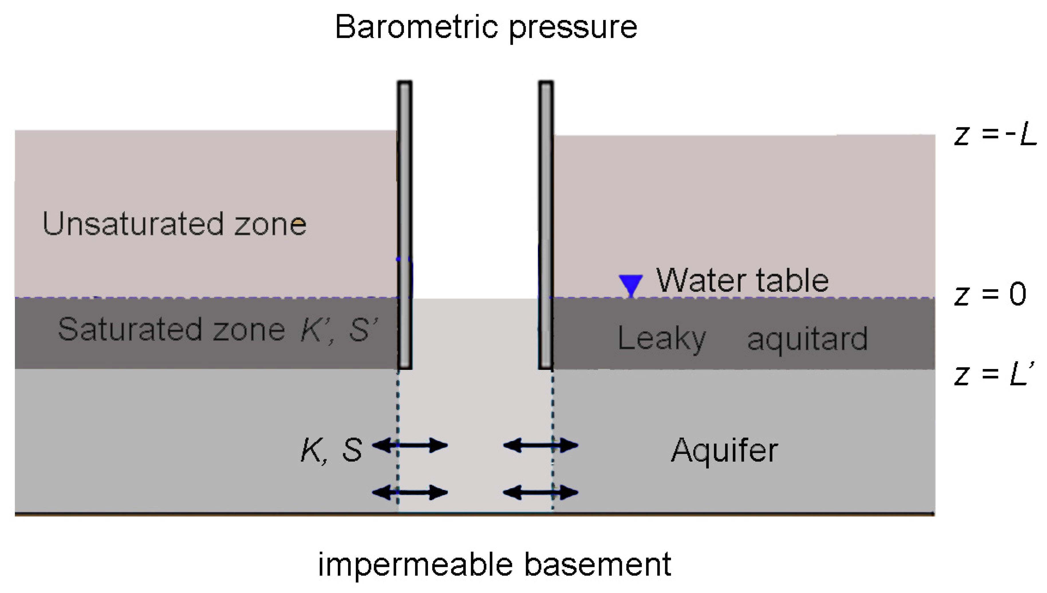
3. Barometric Pressure and Barometric Response

3.1. Barometric Response

The barometric pressure on the Earth’s surface changes with time across large areas and over a wide range of frequencies; hence, the analysis of the response of groundwater to barometric changes may also provide useful information on the hydraulic properties of the groundwater system. The barometric pressure on the Earth’s surface is balanced by the stresses in the solid matrix and the pore pressure in the water. In response to an increase in the barometric load, the increase in water pressure inside an open well that penetrates a confined aquifer (Figure 8) will be greater than the increase in pore pressure in the aquifer, because part of the increased load on the aquifer is supported by the solid matrix. The difference in water pressure will then force the well water to flow into the aquifer. The opposite will occur when the barometric pressure decreases. The response of the water level in an open well is, thus, opposite in sign to the barometric change (Figure 8).

Quantitative analysis of the barometric response began with Jacob [59], who defined the barometric efficiency, BE, as the ratio between the water-level change in the well and the change in barometric pressure (expressed in water height), which is a measure of the aquifer compressibility. The time delay between the water-level response and the barometric change is controlled by the hydraulic diffusivity of both the aquifer and the aquitards (the semi-confining layer). The analysis of the response in the groundwater to barometric changes has been broadly applied to the groundwater system to estimate the hydraulic properties of aquifers and aquitards, e.g., [13,78], and to the studies on earthquake effects on groundwater systems [45,54,62,79].

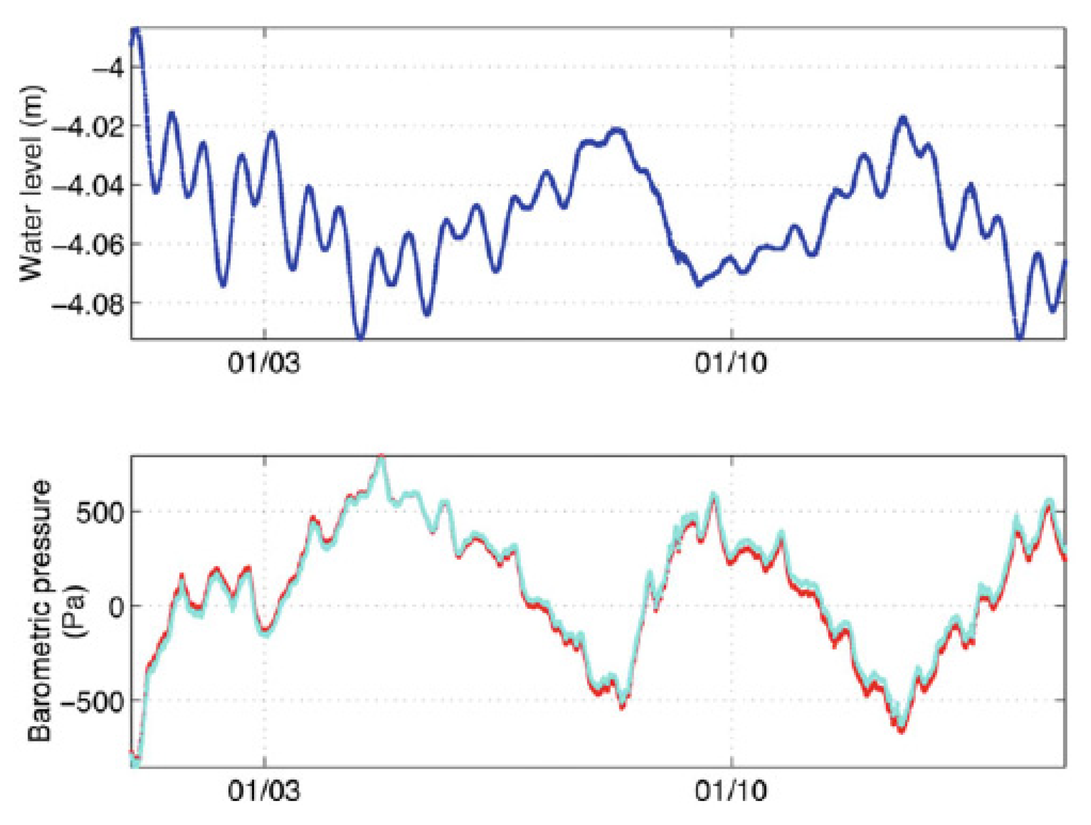
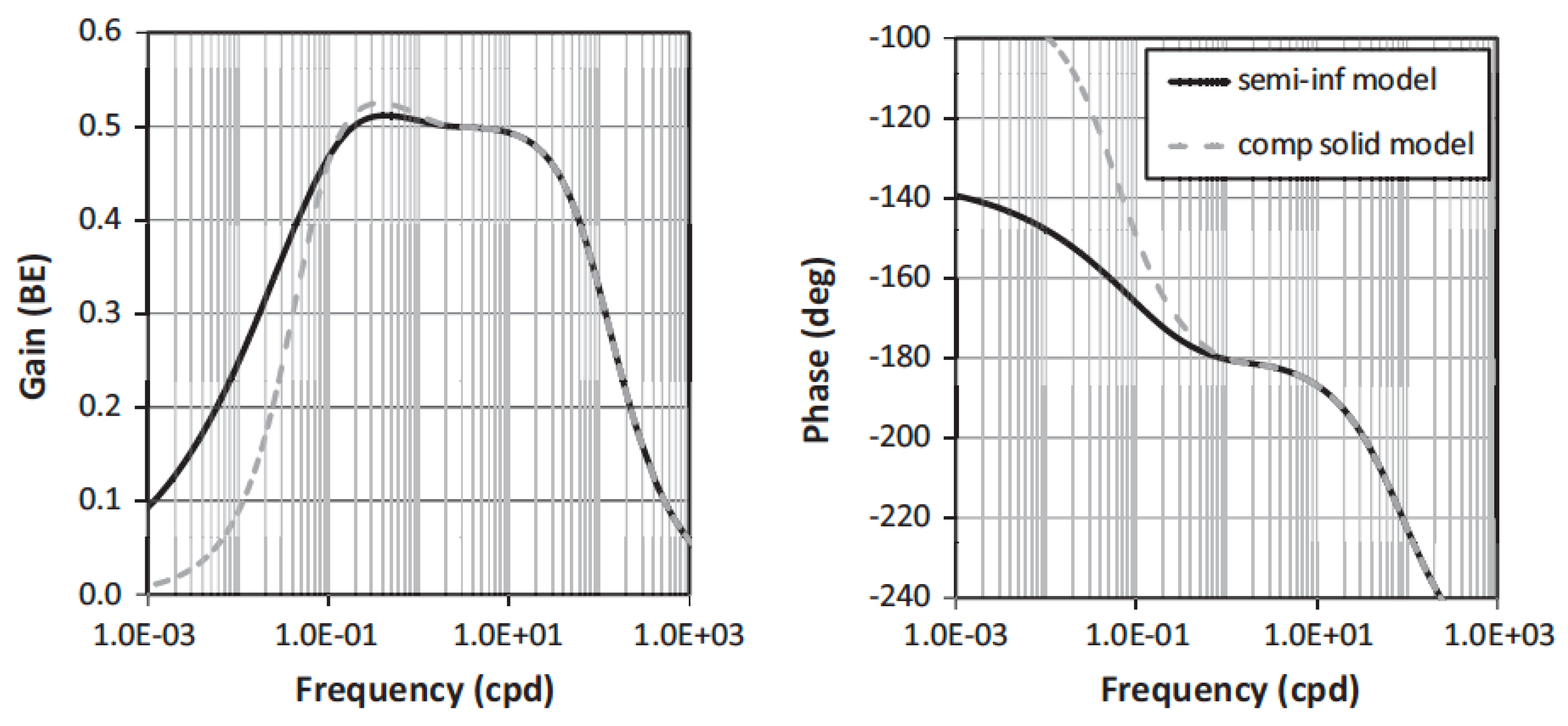
3.2. Barometric Response of the Groundwater Level in Wells

If the aquifer is perfectly confined and has high lateral transmissivity, the response of the water level in a well to a change of barometric pressure is linearly proportional to the barometric change. Since, as noted earlier, most aquifers are not perfectly confined and boreholes have a finite amount of storage, the barometric efficiency depends on the frequency of the applied load. Analysis of this dependency was discussed in several papers, e.g., [13,78,80] and applied to study how the vertical hydraulic conductivity of the aquitard and the horizontal transmissivity of the aquifer may depend on frequency. An advantage in the study of the barometric response of the groundwater is that onsite measurements of barometric pressure are often available to serve as a reference in the analysis.

Rojstaczer [13] expressed the frequency-dependent water-level fluctuation in a borehole in response to changing barometric pressure (Figure 9) as the sum of the fluctuating barometric pressure in the unsaturated zone, the influence of pore pressure in the saturated aquitard, and the flow between the borehole and a semi-confined aquifer:

$$x_o=-\frac{A}{\rho g}+\frac{P_o}{\rho g}-s_o,$$

(12)

where $x_o$, $A,$ $P_o$ and $s_o$ are, respectively, the complex amplitudes of the water-level fluctuation in the borehole, the atmospheric load, the pore pressure at the base of the aquitard, and the drawdown in the well.

For the periodic flow of air between the surface and the water table, Rojstaczer [13] used the differential equation:

$$D_a\frac{{\partial }^2{P}_a}{{\partial z}^2}=\frac{\partial P_a}{\partial t}$$

(13)

with the boundary condition on the Earth’s surface as:

$$P_a\left(z=-L,t\right)=A\cos \left(\omega t\right)$$

(14)

where z = 0 is taken to be at the groundwater table, z = −L is taken to be the Earth’s surface, A is the amplitude of the barometric oscillations at the surface, and $D_a$ is the pneumatic diffusivity in the unsaturated layer, which is assumed to be constant. The solution for air pressure at the water table (z = 0) is [13]:

$$P_a\left(0,t\right)=A\left(M+iN\right) \exp \left(i\omega t\right)$$

(15)

where:

$$M=\frac{2\cosh \left(\sqrt{R_a}\right)\cos \left(\sqrt{R_a}\right)}{\cosh \left(2\sqrt{R_a}\right)+\cos \left(2\sqrt{R_a}\right)},$$

(16)

$$N=\frac{2\sinh \left(\sqrt{R_a}\right)\sin \left(\sqrt{R_a}\right)}{\cosh \left(2\sqrt{R_a}\right)+\cos \left(2\sqrt{R_a}\right)},$$

(17)

and

$$R_a=L^2\omega /2D_a.$$

(18)

Vertical flow is also assumed for the saturated aquitard, with the differential equation:

$$D^{\prime }\frac{{\partial }^{2}P}{\partial z^2}=\frac{\partial P}{\partial t}+A\omega \gamma \sin \omega t,$$

(19)

where $P$ is the excess pore pressure in the saturated aquitard (above the hydrostatic pressure), $D^{\prime }$ is the hydraulic diffusivity of the aquitard, and $\gamma$ is the loading efficiency of the aquitard defined as 1 − BE, i.e.,

$$\gamma =1-\left|x_o\rho g/A\right|.$$

(20)

The upper boundary condition is equal to the barometric pressure at the water table (15), i.e.,

$$P\left(0,t\right)=P_a\left(0,t\right)=A\left(M+iN\right)\exp \left(i\omega t\right).$$

(21)

Rojstaczer [13] simplified the problem by assuming a half space for the saturated aquitard. Thus,

$$P\left(\infty ,t\right)=A\gamma \exp \left(i\omega t\right).$$

(22)

Under these boundary conditions, the solution to (19) at the base of the aquitard ($z=L^{\prime }$) is:

$$P\left(z=L^{\prime }\right)=A\left[\gamma +\left(M+iN-\gamma \right) \exp \left(-\left(1+i\right)\sqrt{R^{\prime }}\right)\right]\exp \left(i\omega t\right),$$

(23)

where:

$$R^{\prime }={L\prime }^2\omega /2D^{\prime }.$$

(24)

For the radial flow between the borehole and the aquifer, the differential equation is [74]:

$$T\left(\frac{{\partial }^{2}s}{\partial r^2}+\frac{1}{r}\frac{\partial s}{\partial r}\right)-\frac{K^{\prime }s}{L^{\prime }}=S\frac{\partial s}{\partial t}$$

(25)

where the small letter s is the ‘drawdown’ near the well, T and S are the transmissivity and storativity of the aquifer, respectively, and $K^{\prime }$ and $L^{\prime }$ are the hydraulic conductivity and the thickness of the semi-confining aquitard, respectively. The boundary conditions are:

$$s\left(\infty ,t\right)=0,$$

(26)

and

$$\underset{r\to r_w}{\lim } \frac{r\partial s}{\partial r}=\frac{\omega r_w^2{x}_o}{2T}\sin \omega t,$$

(27)

where r_w is the well radiusand x_o is the amplitude of the water-level fluctuation in the well produced by the volumetric discharge of the aquifer. Subjected to these conditions, (25) may be solved to yield the drawdown rate in the well [81]:

$$s_w=\frac{i}{2}W{x}_o{K}_o\left\{{\left[W^2\left(S^2+q^{-2}\right)\right]}^{1/4}\exp \left[\frac{i}{2}{\tan }^{-1} \left(qS\right)\right]\right\} \exp \left(i\omega t\right)$$

(28)

where K_o is the modified Bessel function of the second kind of order zero,

$$W=\omega r_w^2/T,$$

(29)

and

$$q=L^{\prime }\omega /K^{\prime }.$$

(30)

Thus, $P_o$ and $s_o$ in (12) are:

$$P_o=A\left[\gamma +\left(M+iN-\gamma \right)\exp \left(-\left(1+i\right)\sqrt{R^{\prime }}\right)\right],$$

(31)

and

$$s_o=\frac{i}{2}W{x}_o{K}_o{\left[W^2\left(S^2+q^{-2}\right)\right]}^{1/4}\exp \left[\frac{i}{2}{\tan }^{-1} \left(qS\right)\right].$$

(32)

Rojstaczer [13] approximated the saturated aquitard by a half-space, which may introduce errors in the predicted barometric response, as explained later. Odling et al. [78] presented an improved model in which the thickness of the aquitard is finite. In this case, the solution for $P_o$ becomes:

$$P_o=A\left[\gamma +\left(M+iN-\gamma \right)\left(E^{\prime }-F^{\prime }\frac{G{E}^{\prime }+H{G}^{\prime }}{G{F}^{\prime }+H{H}^{\prime }}\right)\right],$$

(33)

where M and N are the same as defined in (15) and (16) and, for the aquitard,

$$E^{\prime }=\mathrm{c}\mathrm{o}\mathrm{s}\mathrm{h}\left[\left(1+i\right)\sqrt{R^{\prime }}\right],$$

(34)

$$F^{\prime }=\frac{L^{\prime }}{K^{\prime }}\frac{\sinh \left[\left(1+i\right)\sqrt{R^{\prime }}\right]}{\left[\left(1+i\right)\sqrt{R^{\prime }}\right]},$$

(35)

$$G^{\prime }=-\frac{K^{\prime }}{L^{\prime }}\left[\left(1+i\right)\sqrt{R^{\prime }}\right]\mathrm{s}\mathrm{i}\mathrm{n}\mathrm{h}\left[\left(1+i\right)\sqrt{R^{\prime }}\right],$$

(36)

$$H^{\prime }=E^{\prime }.$$

(37)

For the aquifer, E, F, G and H are similarly defined, with R′ replaced by:

$$R=L^2\omega /2D,$$

(38)

and $L$, $K$ and $D$, respectively, are the corresponding parameters of the aquifer.

The barometric efficiency and the phase of the response are defined as:

$$\mathrm{BE}\left(\omega \right)=\left|x_o\rho g/A\right|,$$

(39)

and

$$\eta \left(\omega \right)=\arg \left(x_o\rho g/A\right).$$

(40)

Figure 10 compares the barometric efficiency and phase of the groundwater response predicted by the two models. For the input parameters (

Table 3. Input parameters for calculating the curves in Figure 10 with both the Rojstaczer [13] model and the Odling et al. [78] model (from [78]).

Parameter	Value
Barometric efficiency, BE (no units)	0.5
Saturated aquitard thickness, L′ (m)	18
Unsaturated aquitard thickness, L (m)	2
Saturated aquitard hydraulic diffusivity, D′ (m2/d)	50
Unsaturated aquitard pneumatic diffusivity, D (m2/d)	10
Aquifer specific storage, Ss(aqf) (m−1)	2.76 × 10−6
Aquitard specific storage, Ss(aqt) (m−1)	6.71 × 10−4
Well radius, rw (m)	0.075

), the predicted barometric efficiency and the phase of the water-level response from the two models [13,78] (are nearly identical at frequencies greater than 1 cpd (Figure 10); at frequencies lower than 1 cpd, however, the predicted phase from the two models diverges, with the difference increasing with decreasing frequency, reaching several tens of degrees at a frequency of 0.01 cpd (Figure 10). This difference may be explained by the ‘skin depth’ of the fluctuating barometric pressure. Assuming a uniform half-space, the depth at which the amplitude of fluctuating barometric pressure decays to 1/e of its surface amplitude is $\delta =\sqrt{2D/\omega }$. For $D$ = 50 m²/day (Table 3) and $\omega$ = 7.3 × 10⁻⁵ s⁻¹ (~1 cpd), where we have $\delta ~4$ m. At $\omega <$ 1 cpd, the ‘skin depth’ of the fluctuating barometric pressure, ~3 $\delta$, exceeds the thickness of the saturated aquitard assumed in Odling’s model (Table 3) and the approximation of the saturated aquitard by a half-space becomes invalid.

3.3. Assessing Earthquake Impact on Groundwater with Barometric Response

A welcome recent development is the utilization of both the tidal and the barometric responses to study earthquake impacts on groundwater systems [45,54,60,82]. The first three of these studies reported changes in the response of the water level in the Zuojiazhuang (ZJZ) well in northern China (Figure 4), during the 2011 Mw9.1 Tohoku earthquake, as discussed in the previous section. Here we compare their analyses of the barometric response and its changes, during the same earthquake.

Zhang et al. [82] showed a nearly constant barometric efficiency of 0.55 before and after the earthquake over the frequency band between 0.07 to 0.6 cpd (left of Figure 11a), and a phase shift slightly less than −180° before the earthquake, but slightly greater than −180° after the earthquake (right of Figure 11a). Zhang et al. [45] re-analyzed the data over the frequency band from 0.02 to 0.6 cpd and showed that, from 0.1 to 0.6 cpd, the response had a nearly constant barometric efficiency of 0.55 before and after the earthquake, similar to that in [82] but, at frequencies below 0.1 cpd, the post-seismic barometric efficiency became lower than that before the earthquake. At a frequency of 0.02 cpd, for example, the barometric efficiency declined from a pre-seismic value of 0.7 to below 0.5. It is reassuring that the results from the two independent analyses are largely consistent over the frequency band, which is common in both studies.

The post-seismic positive phase shift in Zhang et al. [82] (Figure 11a) and the post-seismic decrease in the barometric efficiency in Zhang et al. [45] at frequencies <0.1 cpd are both consistent with the authors’ interpretations of the tidal response of a post-seismic increase in the vertical leakage. Furthermore, He et al. [79] used the groundwater response to Earth tides and barometric pressure, and estimated a high (D ≈ 3 m²/s) hydraulic diffusivity in the fault-damage zone embedded in crystalline rock; they concluded that the combined tidal- and barometric-response method is a robust approach for characterizing the hydrogeological properties of fault-damage zones.

Some recent attempts have used the barometric tides produced by the thermal contraction and expansion of the atmosphere in response to the solar heating of the Earth’s atmosphere. Since these barometric tides and the gravitational tides have the same frequencies, they need to be ‘disentangled’ with special techniques, as discussed by Valois et al. [61]. Furthermore, since these tides have the same frequencies as the solar gravitational tides, S₁ and the S₂ (Table 1), they have often been denoted with the same symbols as the Earth tides, e.g., [30,60], which may introduce some confusion. Figure 12 shows the inverted diffusivity (D′) and loading efficiency (${\gamma }^{\prime }$) of the upper layer of a two-layered aquifer inverted from the response of the groundwater to the barometric tide in a well in Martinique, in the Lesser Antilles archipelago [60], where D′ = K′/$S_s^{\prime }$, and K′ and $S_s^{\prime }$ are, respectively, the vertical hydraulic conductivity and the specific storage of the upper layer. The inverted hydraulic parameters showed significant variations between earthquakes and heavy rainfall, even though these physical properties should be constant when not disturbed by earthquakes or heavy rainfall. Such variations were interpreted by the authors to show ‘long-term evolution’ but these may also be mapping uncertainty and variability in the tidal data.

4. Mechanisms

The significant distinction between the responses observed in different wells and, in the same well, between the responses to different earthquakes (e.g., Figure 6) suggest that different mechanisms cause the changes during earthquakes. For the transient and recoverable co-seismic changes of hydraulic properties, there are two often proposed models: one is the co-seismic removal of gas bubbles from the pores in aquifers [33,83,84,85,86] and the other is the co-seismic removal of colloidal deposits or debris that has clogged pre-existing fractures [4] and reclogged the fractures by accumulating or precipitating new deposits from the flowing groundwater after the earthquakes [4,42,51,87]. These models, where seismic waves dislodge gas bubbles or particles from pores or fractures and then groundwater deposits cause new particles to reclog flow pathways, imply transient and recoverable changes. The time from co-seismic change to recovery ranges from about half an hour in laboratory measurement [88,89,90] to months in nature [42,87].

On the other hand, the orders of magnitude and the irrecoverable changes in permeability at great epicentral distance to great earthquakes (Figure 5 and Figure 6; [45,51]) and at close distance to major earthquakes (Figure 4b; [43]) cannot be explained by the model of clogging and unclogging of pores or pre-existing fractures unless the clogging process is extremely slow. Wang [91] proposed that earthquakes may pressurize the groundwater systems to cause hydro-fractures in the aquifer and the liquefaction of unconsolidated materials. The liquefied sands may be injected into fractures to keep fractures open, and the increased permeability may last for long periods of time. The proposed mechanism enables prolonged upward migration of hot fluids from deep basins, which may be an important process for the subsurface transport of heat and solutes, and useful to understand the safety of groundwater and the security of underground repositories. This model seems to be consistent with field observations at excavated sites of paleo-liquefaction [81,92] where extensive subsurface networks of sand dikes and sills, which represent the conduits for pressurized pore water and sediments to escape from the liquefied layers, were discovered. The geological record also documents liquefied structures in deep sedimentary sequences in the form of homogenized and inverted sand dikes that cut across impermeable barriers to facilitate the expulsion of fluids, e.g., [93,94,95,96]. Seismic profiling in deep sedimentary basins for petroleum exploration has further detected anomalous structures that may be associated with liquefied sediments in the subsurface, e.g., [97,98].

Shi et al. [51] analyzed the frequency content of the surface waves from the two earthquakes using seismic records from a broadband seismometer near the Taiyuan well (Figure 4). They showed that the Rayleigh waves of the Tohoku earthquake have a dominant frequency of ~0.05 Hz, lower by a factor of five than that of the Wenchuan earthquake and suggested that lower frequency seismic waves may be more effective in clearing clogged fractures, resulting in the prolonged increase in the vertical permeability after the Tohoku earthquake. However, the higher frequency seismic waves from the Wenchuan earthquake also caused the prolonged (many years) disruption of the aquitard in the JY well (top row of Figure 1a) near the ruptured fault (Table 1), a transient change in aquitard permeability (K′) in the TY well (top row of Figure 1b) 1115 km from the epicenter, but no change in the aquitard permeability in the ZJZ well (second row of Figure 1b) 1532 km from the epicenter, showing that other mechanisms may also play a role in triggering aquitard disruption.

Zhang et al. [40] found that the water temperature, water level, and flow rate in an artesian well in SW China always show co-seismic step-like increases following earthquakes. Coupled modeling of the flow rate and water temperature indicates that the co-seismic temperature changes are the result of mixing different volumes of water from shallow and deep aquifers, indicating that the vertical permeability was enhanced by earthquakes, consistent with the results from their analysis of the tidal response of groundwater before and after the earthquakes.

Finally, after the 2004 M9.1 Sumatra earthquake in Indonesia, a violent eruption of groundwater occurred in southern China, more than 3000 km from the epicenter, with the maximum height of the eruptive column reaching ~65 m above the ground surface [99,100,101]. Analysis of the tidal response of the groundwater in this well showed that the vertical conductivity of the aquitard increased from 5.5 × 10⁻⁶ to 1.1 × 10⁻⁵ m/s during the earthquake [101]. Yan et al. [101] further inferred that the violent eruption may have been caused by the volumetric expansion of a water–CO₂ mixture from a source in the crust near the erupting well, during the Sumatra earthquake.

5. Suggested Future Studies

The reviewed examples highlight the ability to document and monitor changes in aquifer properties in a passive manner by monitoring water-level responses to tides and barometric pressure. The number of wells and earthquakes studied to date are modest and this limits the ability to identify clear patterns in the magnitude, duration, and mechanism of hydrogeological changes after earthquakes. Open questions, thus, remain about what types of formations are most sensitive to earthquakes, the mechanisms that cause permeability changes, whether there is a frequency dependence in the seismic waves that cause changes, whether there is a threshold strain or strain-rate amplitude for causing changes, and why some changes are recoverable and others are not. Progress in answering these questions may be possible by studying more wells and the responses to more earthquakes.

While the model for the semi-confined aquifer is versatile to provide estimates of the vertical permeability K′ and its change during earthquakes, the current model [38] did not consider wellbore damage (the skin effect) or aquitard storage, which may cause oversimplifications. Gao et al. [102] considered the skin effect and Thomas et al. [60] considered the effect of aquitard storage in their models. Inclusion of both the skin effect and the aquitard storage in the semi-confined model may be needed in the study of the impact of earthquakes on groundwater systems, but this would increase the number of unknowns to five, i.e., K′ and $S_s^{\prime }$ for the aquitard, T and S for the aquifer, and the skin effect. In this case, the inversion of the hydraulic parameters from the phase and amplitude of the M₂ and O₁ tides alone becomes under constrained, and the inclusion of the atmospheric tides may become necessary to constrain the inversion for the evaluation of the hydraulic parameters and their changes during earthquakes.

Multiple models can sometimes explain at least a subset of observations. For example, changes in the phase and amplitude of tidal responses can be modeled with a leaky aquifer or hydraulically transmissive fractures. Independent testing of the inferred changes using well tests may be needed to distinguish between conflicting model interpretations.

Several studies have compiled the impact of earthquakes on groundwater systems as expressed by different co-seismic responses, such as the occurrence of liquefaction, changes in groundwater level, groundwater temperature, stream discharge, spring flow, and the eruptions of geysers and mud volcanoes (see Wang and Manga [20] for a summary). These changes are obviously related to the change in the subsurface permeability. However, the relationship between these co-seismic changes and the co-seismic changes in the tidal response of the groundwater is currently unclear. In the past decade there has been accelerating effort in applying artificial intelligence-based approaches in research on earthquake-related phenomena, e.g., [103,104]. Progress has been made primarily in the study of earthquake prediction, e.g., [103,104,105], earthquake detection, e.g., [106,107], in the estimation of the earthquake’s effect on the groundwater level, e.g., [108], in the detection of possible earthquake precursors [109,110], in the prediction of earthquake hazards [111], and in modeling the hydrological response to earthquakes [112]. To date, however, there has been little effort in applying artificial intelligence-based approaches to the study of earthquake-induced changes in the groundwater response to Earth tides or the barometric pressure. This is probably because, as noted earlier, the numbers of wells and earthquakes studied to date are still modest. With a potential increase in the number of wells and earthquakes, the opportunities to apply artificial intelligence-based approaches to the well data will increase, and may eventually allow us to answer some open questions summarized at the beginning of this section, in particular, what types of formations are most sensitive to earthquakes, the mechanisms that cause permeability changes, whether there is a frequency dependence in the seismic waves that cause changes, whether there is a threshold strain or strain-rate amplitude for causing changes, and why some changes are recoverable and others are not.

Finally, the unconfined aquifer on the top of a groundwater system is usually not fully saturated, but contains an unsaturated zone near the ground surface, which is separated from the saturated zone by the water table. The interfacial tension between the air, water, and solid grains in the unsaturated zone may pull groundwater to rise above the water table to form a zone of negative pore pressure, i.e., the capillary zone, which may significantly affect the tidal response of some aquifers [109,113,114]. The study of the influence of the capillary zone on the tidal response of groundwater, however, is relatively recent and has not yet been applied to understand earthquake impacts.

6. Concluding Remarks

Better management of groundwater resources requires knowledge of the aquifer properties. As shown in numerous studies reviewed in this paper, the hydraulic properties of aquifers are not constant in time and may change significantly during earthquakes. Such changes often create leakage of aquifers, leading to exchanges of groundwater among different aquifers, or between aquifers and the surface water. Some of these changes are long lasting and do not recover to the pre-seismic level after many years. In such cases, the management of groundwater resources based on the knowledge of the pre-seismic aquifer properties may lead to erroneous decisions. Because large earthquakes may occur unexpectedly and because aquifer leakage may cause the spreading of hazardous waste from their repositories, urgent action may often be required. As shown in this review, the tidal and barometric response methods are particularly useful in evaluating the impacts of earthquakes. Their advantages make it possible for large-scale, real-time re-evaluation of the safety of groundwater after large earthquakes. It is the opinion of the authors that real-time and continuous monitoring of groundwater including the tidal and barometric response of the groundwater should be mandatory, particularly in areas prone to natural or induced earthquakes and near the repositories of hazardous waste.

References

1. Castellano, C.; Cucci, L.; Tertulliani, A. Reappraisal of data of hydrological changes associated with some strong historical Italian earthquakes. Geosciences 2023, 13, 55. [Google Scholar] [CrossRef]
2. Institute of Geophysics. CAS (China Earthquake Administration) China Earthquake Catalog; Center for Chinese Research Materials: Washington, DC, USA, 1976; p. 500. (In Chinese) [Google Scholar]
3. Wakita, H. Water wells as possible indicators of tectonic strain. Science 1975, 189, 553–555. [Google Scholar] [CrossRef] [PubMed]
4. Brodsky, E.E.; Roeloffs, E.; Woodcock, D.; Gall, I.; Manga, M. A mechanism for sustained water pressure changes induced by distant earthquakes. J. Geophys. Res. 2003, 108, 2390. [Google Scholar] [CrossRef] [Green Version]
5. Chia, Y.P.; Wang, Y.S.; Wu, H.P.; Chiu, J.J.; Liu, C.-W. Changes of groundwater level due to the 1999 Chi-Chi earthquake in the Choshui River fan in Taiwan. Bull. Seismol. Soc. Am. 2001, 91, 1062–1068. [Google Scholar] [CrossRef] [Green Version]
6. Hurst, A.; Scott, A.; Vigorito, M. Physical characteristics of sand injectites. Earth Sci. Rev. 2011, 106, 215–246. [Google Scholar] [CrossRef]
7. Jonsson, S.; Segall, P.; Pedersen, R.; Björnsson, G. Postearthquake ground movements correlated to porepressure transients. Nature 2003, 424, 179–183. [Google Scholar] [CrossRef]
8. Kitagawa, Y.; Koizumi, N.; Takahashi, M.; Matsumoto, N.; Sato, N. Changes in water levels or pressures associated with the 2004 earthquake off the west coast of northern Sumatra (M9.0). Earth Planets Space 2006, 58, 173–179. [Google Scholar] [CrossRef] [Green Version]
9. Matsumoto, N.; Kitagawa, G.; Roeloffs, E.A. Hydrological response to earthquakes in the Haibara well, central Japan—I. Water level changes revealed using state space decomposition of atmospheric pressure, rainfall and tidal responses. Geophys. J. Int. 2003, 155, 885–898. [Google Scholar] [CrossRef] [Green Version]
10. Quilty, E.; Roeloffs, E. Water level changes in response to the December 20, 1994, M4.7 earthquake near Parkfield California. Bull. Seismol. Soc. Am. 1997, 87, 310–317. [Google Scholar] [CrossRef]
11. Roeloffs, E.A. Poroelastic techniques in the study of earthquake-related hydrogeologic phenomena. Adv. Geophys. 1996, 37, 135–195. [Google Scholar]
12. Roeloffs, E.A. Persistent water level changes in a well near Parkfield, California, due to local and distant earthquakes. J. Geophys. Res. 1998, 103, 869–889. [Google Scholar] [CrossRef]
13. Rojstaczer, S. Determination of fluid flowproperties from the response ofwater levels in wells to atmospheric loading. Water Resour. Res. 1988, 24, 1927–1938. [Google Scholar] [CrossRef] [Green Version]
14. Rojstaczer, S.; Wolf, S. Permeability changes associated with large earthquakes: An example from Loma Prieta, California, 10/17/89 earthquake. Geology 1992, 20, 211–214. [Google Scholar] [CrossRef]
15. Rojstaczer, S.; Wolf, S.; Michel, R. Permeability enhancement in the shallow crust as a cause of earthquake-induced hydrological changes. Nature 1995, 373, 237–239. [Google Scholar] [CrossRef]
16. Sato, T.; Matsumoto, N.; Kitagawa, Y.; Koizumi, N.; Takahashi, M.; Kuwahara, Y.; Ito, H.; Cho, A.; Satoh, T.; Ozawa, K.; et al. Changes in water level associated with the 2003 Tokachi-oki earthquake. Earth Planets Space 2004, 56, 395–400. [Google Scholar] [CrossRef] [Green Version]
17. Sil, S.; Freymueller, J.T. Well water level changes in Fairbanks, Alaska, due to the great Sumatra-Andaman earthquake. Earth Planets Space 2006, 58, 181–184. [Google Scholar] [CrossRef] [Green Version]
18. Wang, C.Y.; Cheng, L.H.; Chin, C.V.; Yu, S.-B. Coseismic hydrologic response of an alluvial fan to the 1999 Chi-Chi earthquake, Taiwan. Geology 2001, 29, 831–834. [Google Scholar] [CrossRef]
19. Wang, C.Y.; Chia, Y. Mechanism of water-level changes during earthquakes near field versus intermediate field. Geophys. Res. Lett. 2008, 35. [Google Scholar] [CrossRef]
20. Wang, C.Y.; Manga, M.; Shirzaei, M.; Weingarten, M.; Wang, L.-P. Induced seismicity in Oklahoma affects shallow groundwater. Seismol. Res. Lett. 2017, 88, 956–962. [Google Scholar] [CrossRef]
21. Whitehead, R.L.; Harper, R.W.; Sisco, H.G. Hydrologic changes associated with the October 28, 1983, Idaho earthquake. Pure Appl. Geophys. 1984, 122, 280–293. [Google Scholar] [CrossRef]
22. Cox, S.C.; van Ballegooy, S.; Rutter, H.K.; Harte, D.S.; Holden, C.; Gulley, A.K.; Lacrosse, V.; Manga, M. Can artesian groundwater and earthquake-induced aquifer leakage exacerbate the manifestation of liquefaction? Eng. Geol. 2021, 281, 1059982. [Google Scholar] [CrossRef]
23. Galli, P. New empirical relationships between magnitude and distance for liquefaction. Tectonophysics 2000, 324, 169–187. [Google Scholar] [CrossRef]
24. Guliyev, I.S.; Huseynov, D.A. Relics of Mud Volcanoes in the Sedimentary Cover of the South Caspian Basin. Lithol. Miner. Resour. 2015, 50, 311–321. [Google Scholar] [CrossRef]
25. Hosono, T.; Yamada, C.; Shibata, T.; Tawara, Y.; Wang, C.Y.; Manga, M.; Rahman, A.T.M.S.; Shimada, J. Coseismic groundwater drawdown along crustal ruptures during the 2016 Mw 7.0 Kumamoto earthquake. Water Resour. Res. 2019, 55, 5891–5903. [Google Scholar] [CrossRef] [Green Version]
26. Manga, M. Origin of postseismic streamflow changes inferred from baseflow recession and magnitude-distance relation. Geophys. Res. Lett. 2001, 28, 2133–2136. [Google Scholar] [CrossRef] [Green Version]
27. Muir-Wood, R.; King, G.C. Hydrological signatures of earthquake strain. J. Geophys. Res. Solid Earth 1993, 98, 22035–22068. [Google Scholar] [CrossRef]
28. Wang, C.Y.; Manga, M. New streams and springs after the 2014 Mw6.0 South Napa earthquake. Nat. Commun. 2015, 6, 7597. [Google Scholar] [CrossRef] [PubMed] [Green Version]
29. Waller, R.M.; Thomas, H.E.; Vorhis, R.C. Effects of the good friday earthquake on water supplies. J. Am. Water Work Assoc. 1965, 57, 123–131. [Google Scholar] [CrossRef]
30. Wang, C.Y.; Barbour, A.J. Influence of pore pressure change on coseismic volumetric strain. Earth Planet. Sci. Lett. 2017, 475, 152–159. [Google Scholar] [CrossRef]
31. Wang, C.Y.; Liao, X.; Wang, L.P.; Wang, C.-H.; Manga, M. Large earthquakes create vertical permeability by breaching aquitards. Water Resour. Res. 2016, 52, 5923–5937. [Google Scholar] [CrossRef] [Green Version]
32. Geballe, Z.M.; Wang, C.Y.; Manga, M. A permeability-change model for water-level changes triggered by teleseismic waves. Geofluids 2011, 11, 302–308. [Google Scholar] [CrossRef]
33. Wang, C.Y.; Wang, C.H.; Manga, M. Coseismic release of water from mountains: Evidence from the 1999 (Mw = 7.5) Chi-Chi, Taiwan, earthquake. Geology 2004, 32, 769–772. [Google Scholar] [CrossRef] [Green Version]
34. Mohr, C.H.; Manga, M.; Wang, C.Y.; Kirchner, J.W.; Bronstert, A. Shaking water out of soil. Geology 2015, 43, 207–210. [Google Scholar] [CrossRef]
35. Mohr, C.H.; Manga, M.; Wang, C.Y.; Korup, O. Regional changes in streamflow after a megathrust earthquake. Earth Planet Sci. Lett. 2017, 458, 418–428. [Google Scholar] [CrossRef] [Green Version]
36. Wang, C.Y.; Wang, C.H.; Kuo, C.Y. Temporal change in groundwater level following the 1999 Mw 7.5 Chi-Chi earthquake, Taiwan. Geofluids 2004, 4, 210–220. [Google Scholar] [CrossRef] [Green Version]
37. Wang, C.Y.; Manga, M. Water and Earthquake; Springer: Cham, Switzerland, 2021; Available online: https://link.springer.com/book/10.1007/978-3-030-64308-9 (accessed on 22 February 2023).
38. Wang, C.Y.; Doan, M.L.; Xue, L.; Barbour, A.J. Tidal response of groundwater in a leaky aquifer—Application to Oklahoma. Water Resour. Res. 2018, 54, 8019–8033. [Google Scholar] [CrossRef]
39. Zhang, S.C.; Shi, Z.M.; Wang, G.C. Comparison of aquifer parameters inferred from water level changes induced by slug test, earth tide and earthquake—A case study in the three Gorges area. J. Hydrol. 2019, 579, 124169. [Google Scholar] [CrossRef]
40. Zhang, S.; Shi, Z.; Wang, G.; Zhang, Z.; Guo, H. The origin of hydrological responses following earthquakes in confined aquifer: Insight from water level, flow rate and temperature observations. Hydrol. Earth Syst. Sci. 2023, 27, 401–415. [Google Scholar] [CrossRef]
41. Barbour, A.J.; Xue, L.; Roeloffs, E.; Rubinstein, J.L. Leakage and increasing fluid pressure detected in Oklahoma’s wastewater disposal reservoir. J. Geophys. Res. Solid Earth 2019, 124, 2896–2919. [Google Scholar] [CrossRef]
42. Elkhoury, J.E.; Brodsky, E.E.; Agnew, D.C. Seismic waves increase permeability. Nature 2006, 441, 1135–1138. [Google Scholar] [CrossRef] [Green Version]
43. Liao, X.; Wang, C.-Y.; Liu, C.-P. Disruption of groundwater systems by earthquakes. Geophys. Res. Lett. 2015, 42, 9758–9763. [Google Scholar] [CrossRef]
44. Wang, C.Y. A new mechanism for earthquake-enhanced permeability. Water Resour. Res. 2022, 58, e2021WR031503. [Google Scholar] [CrossRef]
45. Zhang, Y.; Wang, C.Y.; Fu, L.Y.; Yang, Q.Y. Are deep aquifers really confined? Water Resour. Res. 2021, 57, e2021WR030195. [Google Scholar] [CrossRef]
46. Allègre, V.; Brodsky, E.E.; Xue, L.; Nale, S.M.; Parker, B.L.; Cherry, J.A. Using earthtide induced water pressure changes to measure in situ permeability: A comparison with longterm pumping tests. Water Resour. Res. 2016, 52, 3113–3126. [Google Scholar] [CrossRef]
47. Hung, R.J.; Weingarten, M. Persistent groundwater reduction induced by dynamic stresses from the 2019 Ridgecrest earthquake observed within a fractured aquifer near Ash Meadows, Nevada, USA. Earth Planet. Sci. Lett. 2023, 605, 118034. [Google Scholar] [CrossRef]
48. Qi, Z.; Shi, Z.; Rasmussen, T.C. Time- and frequency-domain determination of aquifer hydraulic properties using water-level responses to natural perturbations: A case study of the Rongchang Well, Chongqing, southwestern China. J. Hydrol. 2023, 617, 128820. [Google Scholar] [CrossRef]
49. Shi, Z.; Wang, G.; Minga, M.; Wang, C.Y. Mechanism of co-seismic water level change following four great earthquakes—Insights from co-seismic responses throughout the Chinese mainland. Earth Planet. Sci. Lett. 2015, 430, 66–74. [Google Scholar] [CrossRef] [Green Version]
50. Shi, Z.M.; Wang, G.C. Aquifers switched from confined to semiconfined by earthquakes. Geophys. Res. Lett. 2016, 43, 11166–111172. [Google Scholar] [CrossRef]
51. Shi, Z.; Wang, C.-Y.; Yan, R. Frequency-dependent groundwater response to earthquakes. J. Hydrol. 2021, 603, 127153. [Google Scholar] [CrossRef]
52. Xue, L.; Li, H.B.; Brodsky, E.E.; Xu, Z.-Q.; Kano, Y.; Wang, H.; Mori, J.J.; Si, J.-L.; Pei, J.-L.; Zhang, W. continuous permeability measurements record healing inside the Wenchuan earthquake fault zone. Science 2013, 340, 1555–1559. [Google Scholar] [CrossRef] [PubMed]
53. Xue, L.; Brodsky, E.E.; Erskine, J.; Fulton, P.M.; Carter, R. A permeability and compliance contrast measured hydrogeologically on the San Andreas Fault. Geochem. Geophys. Geosyst. 2016, 17, 858–871. [Google Scholar] [CrossRef] [Green Version]
54. Zhang, Y.; Wang, C.Y.; Fu, L.Y.; Zhao, B.; Ma, Y. Unexpected far-field hydrological response to a great earthquake. Earth Planet. Sci. Lett. 2019, 519, 202–212. [Google Scholar] [CrossRef]
55. Zhang, Y.; Manga, M.; Fu, L.Y.; Yang, Q.Y.; Cui, Z.D.; Huang, Y. Changes of Hydraulic Transmissivity Orientation Induced by Tele-Seismic Waves. Water Resour. Res. 2022, 58, e2022WR033272. [Google Scholar] [CrossRef]
56. Zhang, Y.; Fu, L.-Y.; Zhu, A.; Zhao, L.; Qi, S.; Huang, T.; Ma, Y.; Zhang, W. Anisotropy and heterogeneity induced by shale in aquifer lithology—Influence of aquifer shale on the leaky model with tidal response analysis. Water Resour. Res. 2023, 59, e2021WR031451. [Google Scholar] [CrossRef]
57. He, A.; Singh, R.P. Coseismic groundwater temperature response associated with the Wenchuan earthquake. Pure Appl. Geophys. 2020, 177, 109–120. [Google Scholar] [CrossRef]
58. Hwang, J.-H.; Yang, C.-W.; Chen, C.-H. Investigations on soil liquefaction during the Chi-Chi earthquake. Soils Found. 2003, 43, 107–123. [Google Scholar] [CrossRef] [Green Version]
59. Jacob, C.E. The flow of water in an elastic artesian aquifer. EOS Trans. AGU 1940, 21, 574–586. [Google Scholar] [CrossRef]
60. Thomas, A.; Fortin, J.; Vitteecoq, B.; Liolette, S. Earthquake and heavy rainfall influence on aquifer properties: A new coupled earth and barometric tidal response model in a confined bi-layer aquifer. Water Resour. Res. 2023; in review. [Google Scholar] [CrossRef]
61. Valois, R.; Rau, G.C.; Vouillamoz, J.-M.; Derode, B. Estimating hydraulic properties of the shallow subsurface using the groundwater response to Earth and atmospheric tides: A comparison with pumping tests. Water Resour. Res. 2022, 58, e2021WR031666. [Google Scholar] [CrossRef]
62. Zhang, H.; Shi, Z.M.; Wang, G.C.; Yan, X.; Liu, C.L.; Sun, X.L.; Ma, Y.C.; Wen, D.G. Different sensitivities of earthquake-ihnduced water level and ydrogeological property variations in two aquifer systems. Water Resour. Res. 2021, 57, e2020WR028217. [Google Scholar] [CrossRef]
63. Doan, M.L.; Brodsky, E.E.; Prioul, R.; Signer, C. Tidal Analysis of Borehole Pressure: A Tutorial; Schlumberger-Doll Research Report; Schlumberger: Cambridge, MA, USA, 2006. [Google Scholar]
64. Wilhelm, H.; WZürn; Wenzel, H.-G. (Eds.) Tidal Phenomena; Lecture Notes in Earth Sciences; Springer: Berlin/Heidelberg, Germany, 1997; Volume 66. [Google Scholar]
65. Agnew, D.C. Earth tides. Treatise Geophys. 2007, 3, 163–195. [Google Scholar]
66. Beaumont, C.; Berger, J. An analysis of tidal strain observations from the United States of America: I. The laterally homogeneous tide. Bull. Seismol. Soc. Am. 1975, 65, 1613–1629. [Google Scholar] [CrossRef]
67. Harrison, J.C. Cavity and topography effects on the measurement of tilt and strain. EOS. Trans. Am. Geophys. Union 1974, 56, 1151. [Google Scholar]
68. Hsieh, P.; Bredehoeft, J.; Farr, J. Determination of aquifer permeability from earthtide analysis. Water Resour. Res. 1987, 23, 1824–1832. [Google Scholar] [CrossRef]
69. Wang, H.F. Theory of Linear Poroelasticity with Applications to Geomechanics and Hydrogeology; Princeton University Press: Princeton, NJ, USA, 2000. [Google Scholar]
70. McMillan, T.C.; Rau, G.C.; Timms, W.A.; Andersen, M.S. Utilizing the impact of Earth and atmospheric tides on groundwater systems: A review reveals the future potential. Rev. Geophys. 2019, 57, 281–315. [Google Scholar] [CrossRef] [Green Version]
71. Cutillo, P.A.; Bredehoeft, J.D. Estimating aquifer properties from the water level response to earth tides. Groundwater 2011, 49, 600–610. [Google Scholar] [CrossRef]
72. Galloway, D.L.; Rojstaczer, S.A. Inferences about formation elastic and fluid flow properties from the frequency response of water levels to atmospheric loads and earth tides: 4th Canadian/American conference on hydrogeology: Fluid flow. In Proceedings of the Heat Transfer and Mass Transport in Fractured Rocks, Banff, AB, Canada, 21–24 June 1988; pp. 100–113. [Google Scholar]
73. Ingebritsen, S.E.; Sanford, W.E.; Neuzil, C.E. Groundwater in Geologic Processes, 2nd ed.; Cambridge University Press: New York, NY, USA, 2006. [Google Scholar]
74. Hantush, M.S.; Jacob, C.E. Non-steady Green’s functions for an infinite strip of leaky aquifers. Trans. Am. Geophys. Union 1955, 36, 101–112. [Google Scholar] [CrossRef]
75. Yang, Q.-Y.; Zhang, Y.; Fu, L.-Y.; Ma, Y.; Hu, J. Vertical leakage occurred after an earthquake: Suggestions for utilizing the mixed flow model. Lithosphere 2021, 2021, 8281428. [Google Scholar] [CrossRef]
76. Hanson, J.M.; Owen, L.B. Fracture orientation analysis by the solid earth tidal strain method. In Spe Annual Technical Conference and Exhibition; OnePetro: Richardson, TX, USA, 1982. [Google Scholar]
77. Liao, X.; Wang, C.-Y.; Wang, Z.-Y. Seasonal change of groundwater response to Earth tides. J. Hydrol. 2022, 612, 128118. [Google Scholar] [CrossRef]
78. Odling, N.E.; Serrano, R.P.; Hussein, M.E.A.; Riva, M.; Guadagnini, A. Detecting the vulnerability of groundwater in semi-confined aquifers using barometric response functions. J. Hydrol. 2015, 520, 143–156. [Google Scholar] [CrossRef]
79. He, G.; Shi, Z.; Rasmussen, T.C.; Qi, Z. Fault zone hydraulic parameter estimation by passive methods using natural forces. Water Resour. Res. 2023, 59, e2022WR033377. [Google Scholar] [CrossRef]
80. Hussein, M.E.; Odling, N.E.; Clark, R.A. Borehole water level response to barometric pressure as an indicator of aquifer vulnerability. Water Resour. Res. 2013, 49, 7102–7119. [Google Scholar] [CrossRef]
81. Obermeier, S.F.; Dickenson, S.E. Liquefaction evidence for the strength of ground motions resulting from late Holocene Cascadia subduction earthquakes, with emphasis on the event of 1700 A.D. Bull. Seismol. Soc. Am. 2000, 90, 876–896. [Google Scholar] [CrossRef]
82. Zhang, H.; Shi, Z.; Wang, G.; Sun, X.; Yan, R.; Liu, C. Large earthquake reshapes the groundwater flow system: Insight from the water-level response to Earth tides and atmospheric pressure in a deep well. Water Resour. Res. 2019, 55, 4207–4219. [Google Scholar] [CrossRef] [Green Version]
83. Beresnev, I.; Gaul, W.; Vigil, R.D. Direct pore-level observation of permeability increase in two-phase flow by shaking. Geophys. Res. Lett. 2011, 38. [Google Scholar] [CrossRef] [Green Version]
84. Crews, J.B.; Cooper, C.A. Experimental evidence for seismically initiated gas bubble nucleation and growth in groundwater as a mechanism for coseismic borehole water level rise and remotely triggered seismicity. J. Geophys. Res. Solid Earth 2014, 119, 7079–7091. [Google Scholar] [CrossRef]
85. Deng, W.; Cardenas, M.B. Dynamics and dislodgment from pore constrictions of a trapped nonwetting droplet stimulated by seismic waves. Water Resour. Res. 2013, 49, 4206–4218. [Google Scholar] [CrossRef]
86. National Research Council. State of the Art and Practice in the Assessment of Earthquake-Induced Soil Liquefaction and Its Consequences; National Academies Press: Washington, DC, USA, 2016. [Google Scholar] [CrossRef]
87. Manga, M.; Beresnev, I.; Brodsky, E.E.; Elkhoury, J.E.; Elsworth, D.; Ingebritsen, S.E.; Mays, D.C.; Wang, C.-Y. Changes in permeability caused by transient stresses: Field observations, experiments, and mechanics. Rev. Geophys. 2012, 50, RG2004. [Google Scholar] [CrossRef]
88. Candela, T.; Marone, E.E.B.C.; Elsworth, D. Laboratory evidence for particle mobilization as a mechanism for permeability enhancement via dynamic stressing. Earth Planet. Sci. Lett. 2014, 392, 279–291. [Google Scholar] [CrossRef] [Green Version]
89. Elkhoury, J.E.; Niemeijer, A.; Brodsky, E.E.; Marone, C. Laboratory observations of permeability enhancement by fluid pressure oscillation of in-situ fractured rock. J. Geophys. Res. 2011, 116, B02311. [Google Scholar] [CrossRef] [Green Version]
90. Faoro, I.; Elsworth, D.; Marone, C. Permeability evolution during dynamic stressing of dual permeability media. J. Geophys. Res. 2012, 117. [Google Scholar] [CrossRef] [Green Version]
91. Wang, C.Y. Liquefaction beyond the near field. Seismol. Res. Lett. 2007, 78, 512–517. [Google Scholar] [CrossRef]
92. Obermeir, S.F. The New Madrid Earthquakes: An Engineering-Geologic Interpretation of Relic Liquefaction Features; US Geological Survey Professional Paper; USGS: New Madrid, MO, USA, 1989; p. 114, 1336-B.
93. Alvarez, W.; Staley, E.; O’Connor, D.; Chan, M.A. Synsedimentary deformation in the Jurassic of southeastern Utah—A case of impact shaking? Geology 1998, 26, 579–582. [Google Scholar] [CrossRef]
94. Huuse, M.; Jackson, C.A.-L.; Van Rensbergen, P.; Davies, R.; Felmings, P.B.; Dixon, R.J. Subsurface sediment remobilization and fluid flow in sedimentary basins: An overview. Basin Res. 2010, 22, 342–360. [Google Scholar] [CrossRef]
95. Sherry, T.J.; Rowe, C.D.; Kirkpatrick, J.D.; Brodsky, E.E. Emplacement and dewatering of the world’s largest exposed sand injectite complex. Geochem. Geophys. Geosys. 2012, 13. [Google Scholar] [CrossRef] [Green Version]
96. Thompson, B.J.; Moore, J.C.; Garrison, R.E. A Reservoir-scale Miocene Injectite near Santa Cruz, California. AAPG Mem. 2007, 87, 151–162. [Google Scholar]
97. Andresen, K.J. Fluid flow features in hydrocarbon plumbing systems: What do they tell us about the basin evolution? Marine Geol. 2012, 332–334, 89–108. [Google Scholar] [CrossRef]
98. Cartwirght, J. Regionally extensive emplacement of sandstone intrusions: A brief review. Basin Res. 2010, 22, 502–516. [Google Scholar] [CrossRef]
99. Che, Y.-T.; Yu, J.-Z.; Liu, C.-L.; Wan, Y.-F.; Luo, S.-Q.; He, Y.-Q.; Xiao, Z.-D. Investigation and analysis to co-seismic blowout in Chagan well. Seismol. Geol. 2009, 31, 226–232. [Google Scholar] [CrossRef]
100. Wang, C.Y.; Manga, M. Hydrogeologic responses to earthquakes and a general metric. Geofluids 2010, 10, 206–216. [Google Scholar]
101. Yan, X.; Shi, Z.; Wang, C.Y.; Ingebritsen, S.E.; Manga, M. Violent groundwater eruption triggered by a distant earthquake. Geophys. Res. Lett. 2022, 49, e2022GL101239. [Google Scholar] [CrossRef]
102. Gao, X.; Sato, K.; Horne, R. N General solution for tidal behavior in confined and semiconfined aquifers considering skin and–wellbore storage effects. Water Resour. Res. 2020, 56, e2020WR027195. [Google Scholar] [CrossRef]
103. Beroza, G.C.; Segou, M.; Mostafa Mousavi, S. Machine learning and earthquake forecasting—Next steps. Nat. Commun. 2021, 12, 4761. [Google Scholar] [CrossRef]
104. Galkina, A.; Grafeeva, N. Machine Learning Methods for Earthquake Prediction: A Survey. In Proceedings of the Fourth Conference on Software Engineering and Information Management (SEIM-2019), Saint Petersburg, Russia, 13 April 2019; full papers. p. 25. [Google Scholar]
105. Mignan, A.; Broccardo, M. Neural Network Applications in Earthquake Prediction (1994–2019): Meta- Analytic and Statistical Insights on Their Limitations. Seismol. Res. Lett. 2020, 91, 2330–2342. [Google Scholar] [CrossRef]
106. Mousavi, S.M.; Ellsworth, W.L.; Zhu, W.; Chuang, L.Y.; Beroza, G.C. Earthquake transformer—An attentive deep-learning model for simultaneous earthquake detection and phase picking. Nat. Commun. 2020, 11, 3952. [Google Scholar] [CrossRef] [PubMed]
107. Perol, T.; Gharbi, M.; Denolle, M. Convolutional neural network for earthquake detection and location. Sci. Adv. 2018, 4, e1700578. [Google Scholar] [CrossRef] [Green Version]
108. Yokoo, K.; Ishida, K.; Nagasato, T.; Kawagoshi, Y.; Ito, H. Reconstruction of groundwater level at Kumamoto, Japan by means of deep learning to evaluate its increase by the 2016 earthquake. In IOP Conference Series: Earth and Environmental Science; Iop Science: Bristol, UK, 2021; Volume 851, p. 012032. [Google Scholar]
109. Wang, C.Y.; Zhu, A.Y.; Liao, X.; Manga, M.; Wang, L. Capillary effects on groundwater response to Earth tides. Water Resour. Res. 2019, 55, 6886–6895. [Google Scholar] [CrossRef]
110. Yan, X.; Shi, Z.; Wang, G.; Zhang, H.; Bi, E. Detection of possible hydrological precursor anomalies using long short-term memory: A case study of the 1996 Lijiang earthquake. J. Hydrol. 2021, 599, 126369. [Google Scholar] [CrossRef]
111. Gitis, V.G.; Derendyaev, A.B. Machine learning methods for seismic hazards forecast. Geosciences 2019, 9, 308. [Google Scholar] [CrossRef] [Green Version]
112. Scorzini, A.R.; Bacco, M.D.; De Luca, G.; Tallini, M. Deep learning for earthquake hydrology? Insights from the karst Gran Sasso aquifer in central Italy. J. Hydrol. 2023, 617, 129002. [Google Scholar] [CrossRef]
113. Liang, X.Y.; Wang, C.Y.; Ma, E.Z.; Zhang, Y.K. Effects of unsaturated flow on hydraulic head response to Earth tides—An analytical model. Water Resour. Res. 2022, 58, e2021WR030337. [Google Scholar] [CrossRef]
114. Zhang, J.; Liang, X.; Wang, C.Y. Capillary impact on tidal response of groundwater in two-dimensional unconfined aquifers with finite thickness, anisotropy, and borehole storage—An analytical model. Water Resour. Res. 2023; in press. [Google Scholar]
Figure 1. (a) A rotating Earth, with the center at O and an average radius a, deforming under the gravitational attraction of the Moon with the center at P, separated by a distance R. N is a point on the Earth’s surface at latitude α (not to scale). (b) Schematic diagram of a groundwater well that opens to a semi-confined aquifer, with thickness b and hydraulic conductivity K, overlain by a leaky aquitard with thickness b′ and hydraulic conductivity K′, which in turn is overlain by an unconfined aquifer. The vertical dashed line on the left shows the well axis, located at r = 0. Moreover, h is the hydraulic head of groundwater in the aquifer, h is the hydraulic head of groundwater at a large distance from the well, and rc and rw, respectively, are the radii of the well casing and the screened well (not to scale).
Water 15 01327 g001
Figure 2. Time series of (a) raw data for the groundwater level above the mean sea level in a USGS Oklahoma monitoring well that opens to the Arbuckle aquifer at a depth of ~1 km below the surface, (b) drift in the groundwater level that was removed, (c) tides in the remaining groundwater level after the drift was removed, (d) phase shift of the water-level response to the M2 and S2 tides referenced to the local tidal volumetric strain, (e) amplitude of water-level response (hw,o) to the M2 and S2 tides, and (f) the ratio between the amplitude of the water-level response and the amplitude of the volumetric tidal strain (εo) response to the M2 and S2 tides. Computed using Baytap08 (from [38]).
Water 15 01327 g002
Figure 3. (a) Locations of the USGS Oklahoma deep monitoring wells (red circle at top right corner), Arbuckle disposal wells (blue dots), shallow USGS and OWRB wells, and the epicenters of three 2016 earthquakes with an M ≥ 5. (b) Simplified diagram of the major geologic units in the USGS Oklahoma deep well.
Water 15 01327 g003
Figure 4. (a) Locations of the Piño Flat Observatory and earthquake epicenters in the study by Elkhoury et al. [42] (b) Locations of the Jiangyou well and the epicenter of the Wenchuan earthquake in the study by Liao et al. [43]. (c) Locations of the Taiyuan well (TY) and the Zuojiazhuang well (ZJZ), and the epicenters of the Wenchuan and the Tohoku earthquakes in the studies by Shi et al. [17] and Zhang et al. [45]. (d) Locations of the Fond Lahaye borehole and earthquake epicenters in the study by Thomas et al. [60].
Water 15 01327 g004
Figure 5. (a) Transient and reversible changes in the response of the groundwater to the M2 tide during many earthquakes observed in two wells (CIB and CIC) in southern California (from [42]. (b) Tidal response before and after the 2008 M7.9 Wenchuan earthquake (red arrow) in the JY (Jiangyou) well in Sichuan, China. The co-seismic changes did not return for many years after the earthquake, while the tidal responses in the same well to many small earthquakes (black arrows) were transient and reversible (from [43]).
Water 15 01327 g005
Figure 6. (a) Phase shift and amplitude ratio of the response of the groundwater in the Taiyuan (TY) well to the M2 tide from 2007 to 2017 (from [51]). Notice the distinct difference between the changes after the M7.9 Wenchuan earthquake and those after the M9.2 Tohoku earthquake. (b) Phase shift and amplitude ratio of the response of the groundwater in the Zuojiazhuang (ZJZ) well to both the M2 and the O1 tides from 2008 to 2015 (from [45,75]). Notice also, the distinct difference between the changes after the M7.9 Wenchuan earthquake and those after the M9.2 Tohoku earthquake.
Water 15 01327 g006
Figure 7. Interpretation of the tidal response of the groundwater in the Taiyuan (TY) well and the Zuojiazhuang (ZJZ) well, before and after earthquakes, using the semi-confined aquifer model. (a) For the TY well, only the vertical conductivity of the aquitard (K′) was estimated (modified from [51]. (b) For the ZJZ well, both the vertical conductivity of the aquitard and the horizontal transmissivity (T) and storativity (S) of the aquifer were estimated (modified from [45,75]).
Water 15 01327 g007
Figure 8. Water level recorded in the CIB well by the Piñon Flat Observatory and the barometric pressure on site during the first 15 days of 1999 (modified from [63]).
Water 15 01327 g008
Figure 9. Schematic diagram showing an aquifer and a semi-confining layer (aquitard), the borehole and groundwater flow in response to changing barometric pressure, where K and K′ and S and S′ are, respectively, the hydraulic conductivity and the storativity of the aquifer and aquitard (modified from [13]).
Water 15 01327 g009
Figure 10. Comparison of the BRF gain (left) and phase (right) curves between the model of Rojstaczer [13] using a semi-infinite model for the saturated confining layer (solid black curve), and the modified model of Odling et al. [78] for a saturated confining layer with finite thickness (dashed grey curve). The input parameters for the two models are listed in Table 3 (from [78]).
Water 15 01327 g010
Figure 11. (a) Barometric efficiency and phase shift in the ZJZ well before and after the Tohoku earthquake, plotted against frequency (from [39]). Negative phase shifts indicate that the water-level response lags behind the change in atmospheric pressure. The colored curves show the best fitting curves using the model of Rojstaczer [13]. (b) Barometric efficiency in the ZJZ well before (grey circles) and after (red circles) the Tohoku earthquake, plotted against frequency between 0.02 to 0.6 cpd (modified from [45]). The phase shift is not available in [45].
Water 15 01327 g011
Figure 12. Evolution of (a) the vertical diffusivity D′ defined as K′/ S s , where S s is the specific storage of the top layer in a two-layered aquifer and (b) is the loading efficiency γ′ of the top layer inverted from the response of the groundwater to the barometric tides in a well in Martinique, in the Lesser Antilles archipelago [60]. The orange circles correspond to the results of the pumping tests. The vertical brown lines correspond to earthquakes, the vertical blue lines correspond to heavy rainfall events, and the orange/green rectangles to the pumping operation in the well.
Water 15 01327 g012