Article

Groundwater Contamination Site Identification Based on Machine Learning: A Case Study of Gas Stations in China

1
School of Environment, Harbin Institute of Technology, Harbin 150090, China
2
School of Environmental Science and Engineering, Southern University of Science and Technology, Shenzhen 518055, China
3
Technical Center for Soil, Agriculture and Rural Ecology and Environment, Ministry of Ecology and Environment, Beijing 100012, China
4
Chinese Academy of Environmental Planning, Beijing 100043, China
5
Engineering Innovation Center of SUSTech (Beijing), Southern University of Science and Technology, Beijing 100083, China
*
Author to whom correspondence should be addressed.
Water 2023, 15(7), 1326; https://doi.org/10.3390/w15071326
Submission received: 3 March 2023 / Revised: 26 March 2023 / Accepted: 27 March 2023 / Published: 28 March 2023

Abstract

:
Accurately identifying groundwater contamination sites is vital for groundwater protection and restoration. This study aims to use a machine learning (ML) approach to identify groundwater contamination sites with total petroleum hydrocarbons (TPH) as target contaminants in a case study of gas stations in China. Firstly, six classical ML algorithms, including logistic regression, decision tree, gradient boosting decision tree (GBDT), random forest, multi-layer perceptron, and support vector machine, were applied to develop the identification models of TPH-contaminated groundwater with 40 features and the performances were compared. The comparison results showed that the GBDT model achieves the best prediction performance, with F1 score of 1 and AUC value of 1. Next, Bayesian optimization optimized GBDT (BO-GBDT) was conducted to further decrease the training time from 19,125 s to 513 s while maintaining the same prediction performance (F1 score = 1, AUC = 1). Finally, Shapley additive explanations (SHAP) analysis was performed on the BO-GBDT model. The SHAP results displayed that the critical feature variables in the BO-GBDT model include wind, population, evaporation, total potassium in the soil, precipitation, and leakage accident. This study demonstrated that BO-GBDT is one satisfactory model to identify groundwater TPH-contamination at gas stations. The method proposed in this study has the potential to be applied to other types of groundwater contamination sites.

1. Introduction

The identification of potentially contaminated sites is crucial for the management of contaminated sites and the protection of public health [1]. Given the mobility of groundwater and the difficult-to-repair nature of contamination, the deterioration of groundwater quality due to point source pollution, represented by various industrial and commercial sites, is attracting widespread concern [2,3]. There are over 2.5 million potentially contaminated sites in Europe [3]. In Asia and the USA, new contamination sites are being identified every day [4]. China is estimated to have over 500,000 contaminated sites [5]. Therefore, identifying groundwater contamination sites has become a research hotspot [6].
Current methods for identifying groundwater contamination sites include site history review, field survey and sampling analysis, and interviews [6]. Site history review refers to the search for documents relating to original buildings on the site from environmental and health agencies, associations, unions, and so on [7]. However, historical documents are not always available, especially for sites with long histories. In addition, this method is time-consuming for a large number of sites. Field surveys and sampling analysis have the advantage of maximizing the accuracy of the findings. However, each site requires multiple samples to be collected for laboratory analysis and therefore requires a significant investment of workforce, money, and time [8]. In the interview method, information about the site is obtained by interviewing the site manager, owner, government personnel, and residents around the site to judge the site’s contamination. The drawback of this method is its subjectivity, which may be related to the gender, age, profession, and standpoint of the interviewees, and has a high degree of uncertainty [9,10,11].
Data science methods, represented by machine learning, have attracted significant attention in recent years. The primary purpose of machine learning is to evaluate or predict objectives after training a model with data in specific conditions. The advantage of machine learning is that hidden associations in the data can be learned through automatic mathematical analysis [12]. Currently, many machine learning algorithms are applied to solve groundwater-related problems. Six of these algorithms have been reported to be widely applied, including Logistic regression (LR), decision tree (DT), gradient boosting decision tree (GBDT), random forest (RF), multi-layer perceptron (MLP), and support vector machine (SVM). For example, in the Saladin Province of Iraq, LR was applied to assess groundwater nitrate contamination levels [13]. A DT model was developed to classify groundwater quality in the Ardebil aquifer, Northwest Iran [14]. Spatially distributed feature variables related to arsenic and manganese flows were selected for the GBDT model to obtain areas of high arsenic and manganese in the northern USA [15]. RF, LR, and MLP algorithms were used to model fluoride in groundwater in Datong Basin, China [16]. Four models, including MLP and SVM, were developed to estimate groundwater TDS in the East Azerbaijan Province [17]. Recent researches on identifying groundwater contamination using machine learning mainly focused on the identification of contamination source or intensity in a specific contaminated site. For example, self-organizing map algorithm was applied to identify the source of sulfate in groundwater of an abandoned mine [18]; the Bayesian and machine learning method was used to invert the contamination source release intensity and duration in a hypothetical case study [19]; the deep learning algorithms based on Long-Short Term Memory networks were utilized to identify the contamination source, initial release period, and release intensity in a hypothetical case study with irregular boundaries [20]. However, to our knowledge, few studies have been reported on using machine learning methods to identify potential groundwater contamination sites, especially hybrid machine learning models. Moreover, only a few studies have shown concern for explanatory analyses of the results.
Due to leaks from storage tanks or pipelines, groundwater contamination at gas stations is attracting significant attention worldwide [21]. Relevant reports indicated there might be about 242,000 leaking gas station storage tanks in the EU with contamination from leaks [22]. Four hundred ninety-five thousand leaking gas station storage tanks have been reported in the United States until 2010 [23]. There are 27,000 gas stations in Brazil with possible soil and groundwater contamination from oil spills [24]. There are over 120,000 gas stations in China, located in commercial and residential areas, urban traffic arteries, and highways; some are even in water sources and nature reserves. Total petroleum hydrocarbon (TPH) is one of the primary contaminants in groundwater from gas stations [22,25]. Aromatic hydrocarbons in TPH are carcinogenic, teratogenic, and mutagenic [26]. The China Geological Survey conducted a survey of some gas stations in Tianjin province. The results showed that the detection rate of TPH in groundwater samples was 85%, and the exceedance samples accounted for 40% of the total groundwater samples. Therefore, TPH was set as the target contaminant in this study, and Chinese gas station sites were set as the study area.
This study aimed to develop machine learning models based on multi-source data to identify the current status of groundwater TPH contamination under gas stations in China. LR, DT, GBDT, RF, MLP, and SVM were determined as the machine learning algorithms used in this study. Forty feature variables from the field survey and database were considered as input variables for machine learning to train and test the models. The optimization effect of Bayesian optimization (BO) was also examined, and the importance of feature variables was discussed using the Shapley additive explanations (SHAP) method.

2. Materials and Methods
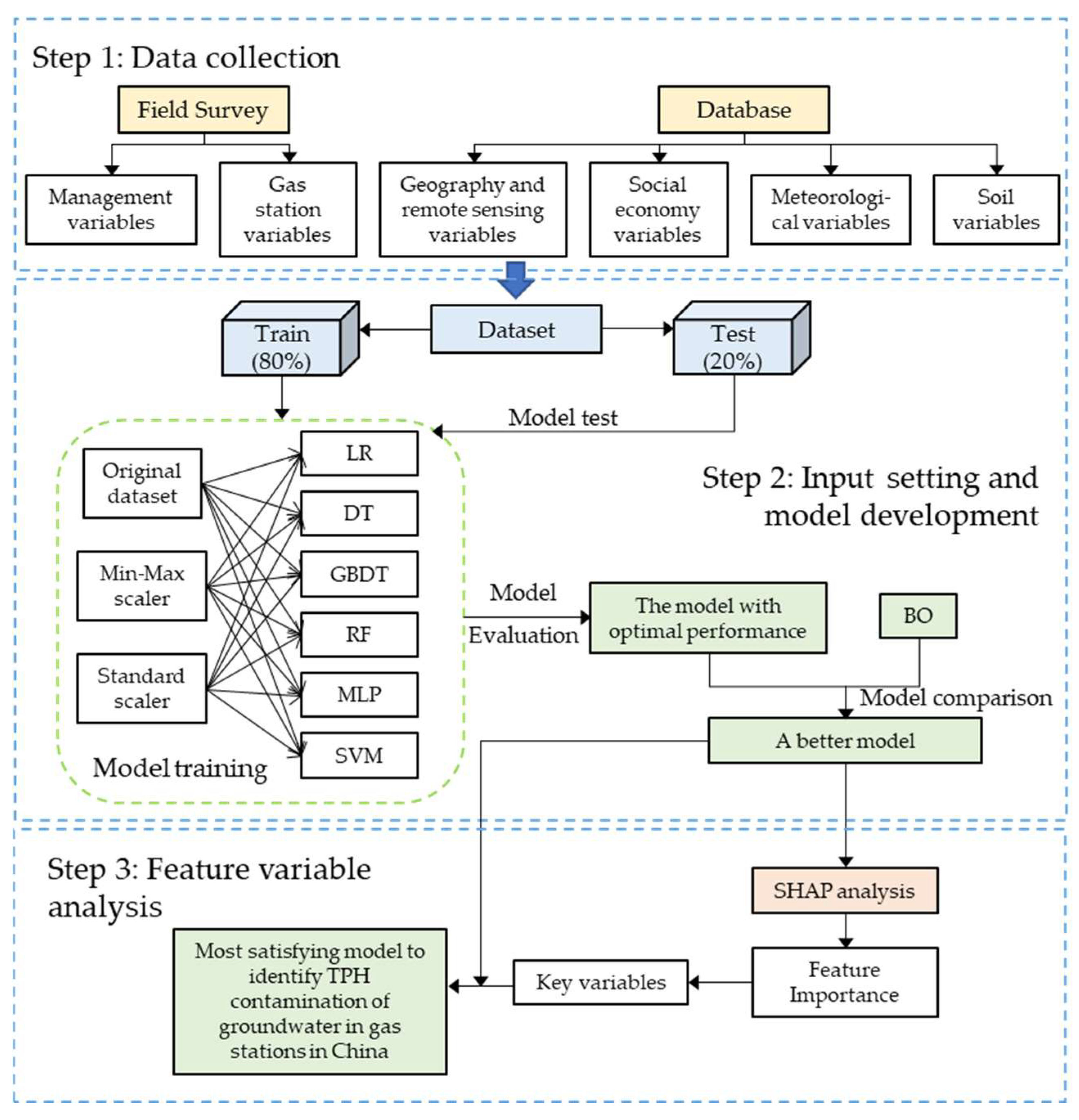
2.1. Methodology

As shown in Figure 1, there are three steps in the framework for developing models for groundwater contamination site identification. Firstly, data collection was conducted simultaneously from the field survey and database. Subsequently, six different machine learning models were built based on a training dataset. Three approaches (original dataset, min-max scaler, standard scaler) were used for data pre-processing. The model with the optimal result was selected according to model evaluation and was compared with the Bayesian optimization (BO) hybrid model to determine a better one. Finally, the feature variables were analyzed using the SHAP method to obtain the key variables. These key variables were combined with the optimal model obtained in step 2 to obtain the most satisfying model to identify groundwater TPH contamination sites.

2.2. Data

Field surveys and groundwater sampling were conducted at 103 gas stations in 24 regions of China following the requirements of the technical guidelines (HJ 25.1-2014) issued by the Ministry of Ecology and Environment of China. The sampling was carried out from 2017 to 2019. Sample collection, storage, transportation, and testing were determined according to guides issued by the Chinese authorities [27,28,29]. The groundwater TPH contamination of 103 gas stations was finally obtained as the target variable for machine learning in this study. Eighty-three gas stations belonged to the “uncontaminated” category, while the other twenty belonged to the “contaminated” category.
The factors affecting TPH contamination of groundwater at gas stations were considered, and the available information was aggregated into the feature variables dataset for this study. The selection of feature variables is based firstly on authenticity, accessibility, completeness, and diversity of the data. The feature variables include six categories: management variables, gas station variables, geography and remote sensing variables, social economy variables, meteorological variables, and soil variables, with a total of 40 variables. All variables may reflect some association with groundwater contamination. Key investigation list (KIL), a management variable, reflected a greater risk of contamination around the gas station. The construction time, a gas station variable, was associated with groundwater contamination at the gas station. The distance to the nearest lake (dist_lake) and distance to the nearest river (dist_river) in the geographic and remote sensing variables might influence the status of groundwater recharge and runoff. Among the social economy variables, the night light index (NLI), population, and GDP correspond to the intensity of human activity, which might be a source of anthropogenic pollution of groundwater. Meteorological variables may influence groundwater recharge and discharge; for example, precipitation is usually positively correlated with vertical recharge and annual sunshine affects groundwater in many aspects such as precipitation and evaporation. The soil related variables are also included, considering the closest contact between soil medium and groundwater. To sum up, these variables come from different sources and reflect the role of the natural environment and human activities and are therefore included. Table 1 shows detailed information on these feature variables, including category, name, description, and type.

2.3. Machine Learning Approach

2.3.1. Models

Here, we briefly introduce the basic principles of the six algorithms (LR, DT, GBDT, RF, MLP, SVM), the detailed principles of which can be found in the attached reference. LR is one of the most classical statistical machine learning models. LR can make categorical predictions from several selected categorical, discrete, or continuous variables and is a suitable technique for predicting binary outcomes [30,31]. Based on a logistic function, LR maps the linear regression results to the interval [0, 1] [32]. DT is a machine learning algorithm based on a tree structure that can reveal complex relationships that are difficult to identify with linear statistical models [33]. The tree includes the root, internal, and leaf nodes. During training, the role of the nodes is to test and assign the feature variable for each input until it reaches the leaf nodes. Each leaf node represents a class of instances [34]; for example, this study represents two classes of TPH out of threshold or not out of threshold. GBDT is an ensemble learning algorithm based on DT consisting of multiple trees. Therefore, it combines crucial advantages of the DT algorithm [35]. The basic idea of GBDT is boosting mechanism. A new tree is trained with the original feature variables in each iteration. This new tree will fit the residuals left by the previous tree, thus continuously reducing the model error [36]. Therefore, the number of trees (n_estimators) is one of the critical hyperparameters of the algorithm. RF is another ensemble learning algorithm based on DT that has been widely modeled in recent years [37]. Unlike GBDT, the idea of RF is bagging. In RF, each tree is trained using a different part of the same training set, meaning each tree learns different samples. A vote of all trees generates the final result of RF. This sampling mechanism allows RF to circumvent the effects of noise in the data [38]. MLP, also known as artificial neural networks, has a long history in groundwater modeling [39]. The MLP model consists of an input, hidden, and output layer. Neurons characterized by weights and biases interconnect these layers. The input layer is to input data, and the output layer is the target of the model prediction. An activation function is embedded in the hidden layer to transform the deviation-weighted summation of the layer to the next layer until it reaches the output layer [40]. Therefore, selecting an appropriate activation function plays an important role in the training of the MLP. In addition, the number of layers and neurons in each hidden layer constitute the hidden layer size, and experiments are needed to obtain the optimal hyperparameter settings. Finally, SVMs are a class of generalized linear classifiers that perform binary data classification in a supervised learning manner. In the binary classification problem investigated in this study, SVMs attempt to locate a hyperplane in the n-dimensional input space that can separate the data points into two distinct classes. The boundaries of this hyperplane (called decision boundaries) also have to be as large as possible to make reliable classification predictions [41].
The computer configuration used to perform the experiments was CPU Core i7-6820HQ, 48 GB of RAM, and Windows 10 as the operating system. We used the Scikit-learn toolkit in Python to perform machine learning modeling (https://scikit-learn.org/stable/index.html (accessed on 3 January 2023)). The GridSearchCV module in Scikit-learn was called to determine the best hyperparameters for different algorithms and optimize the model’s performance. We first identified the critical hyperparameters of each algorithm and the search scope of GridSearchCV through a literature review in conjunction with the problem of this study. GridSearchCV performs an exhaustive search for a specified machine learning algorithm within a hyperparameter search range with an exhaustive search. Afterward, GridSearchCV uses the adjusted hyperparameters to train the learner to find the most accurate parameter in the validation set from all parameters. Here, the validation set is generated by cross-validation with k = 10. The descriptions and ranges of the critical hyperparameters for the different algorithms are shown in Table 2.
Although GridSearchCV is guaranteed to obtain the most satisfying hyperparameters within a specified range of parameters, this advantage also has the disadvantage of being time-consuming. Therefore, after executing GridSearchCV and recording the results, the best-performing machine learning algorithm was selected. BO was introduced to tune and compare the machine learning algorithms with GridSearchCV results, including model performance and time consumption. BO is a powerful sequential optimization tool widely applied in machine learning modeling for its ability to obtain the best hyperparameter values quickly [47]. BO allows for mastery of prior knowledge, i.e., incorporating historical information in the iterative process and avoiding redundant and unnecessary evaluation of the objective function c(x) [48,49]. In this study, the execution of BO is implemented by the bayes_opt toolkit.

2.3.2. Input Setting and Feature Importance Analysis

The dataset was randomly divided into a training set and a test set by applying the leave-out method at 80–20%. The model’s training is performed on the training set, and the test set checks the model’s generalization ability. We first used all 40 feature variables as input to machine learning to examine the performance of the algorithms. Three different continuous variable pre-processing methods were considered to examine the effect of pre-processing on model performance. The three continuous variable pre-processing methods are original dataset (OD), Min-Max Scaler (MMS, Equation (1)), and standard scaler (SS, Equation (2)):
X n e w = X X m i n X m a x X m i n
where Xnew represents the scaled value, X is the original value to be scaled. Xmax and Xmin represent the maximum and minimum values in the feature variables, respectively.
X n e w = X μ σ
where μ and σ are the mean and standard deviation of the feature variables.
SHAP is a game-theoretic method that can be applied to interpret the output of machine learning models [50]. SHAP interprets the output of a model as the sum of the actual values attributed to each input feature variable and is an additive feature attribution method [51]. The detail of the computational principles of SHAP can be found in the attached reference [52]. In this work, SHAP was applied to explain the attribution of the model based on a well-established machine learning model for groundwater TPH-contaminated site identification at gas stations.

2.3.3. Model Evaluation

F1 score and area under curve (AUC) were chosen to evaluate the performance of models. Gas stations with TPH-contaminated groundwater are marked as 1 and uncontaminated as 0. If the predicted result and actual value are both 1, the station is classified as a True Positive (TP); while, if the predicted result and actual value are both 0, the station is classified as a True Negative (TN). Conversely, if the predicted result is 1 but the actual result is 0, the station is classified as a False Positive (FP), and if the predicted result is 0 but the actual result is 1, the station is classified as a False Negative (FN). Precision refers to the proportion of results with a predicted value of 1 corresponding to an actual value of 1, i.e., TP/(TP + FP). In contrast, recall refers to the proportion of samples with an actual value of 1 with a predicted outcome of 1, i.e., TP/(TP + FN). F1 score is taken to be in the interval [0,1], the larger, the better. According to Equation (3), the F1 score can be calculated as follows:
F 1   score = 2 × precision × recall precision + recall
AUC is calculated based on the receiver operating characteristic curve (ROC), which consists of recall and 1-specificity for different classification probability thresholds. AUC is the area bounded by the ROC curve and the x-axis, x = 1. AUC is within the range [0.5, 1], with larger values indicating better model performance.
In addition, this study evaluates the training speed according to the time consumption, aiming to obtain the most efficient model.

3. Results and Discussion

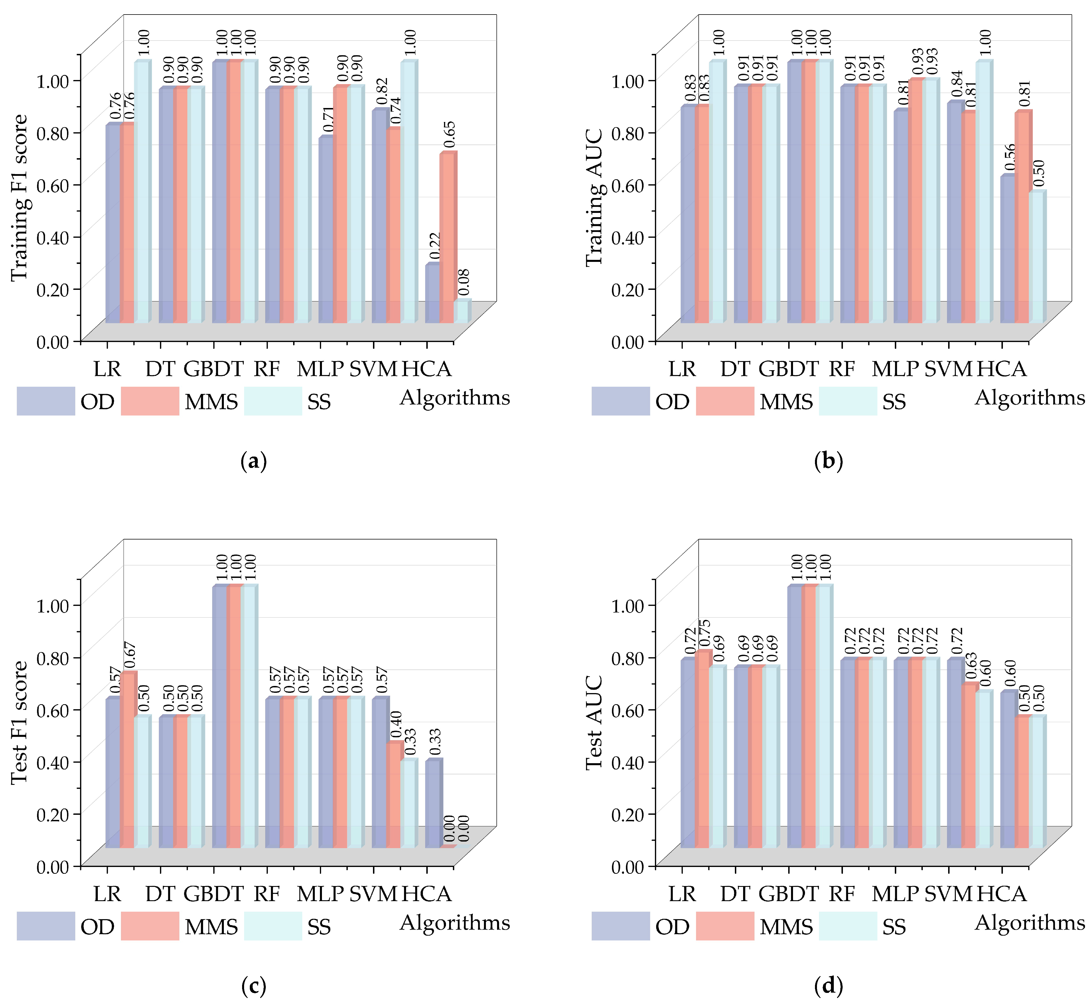
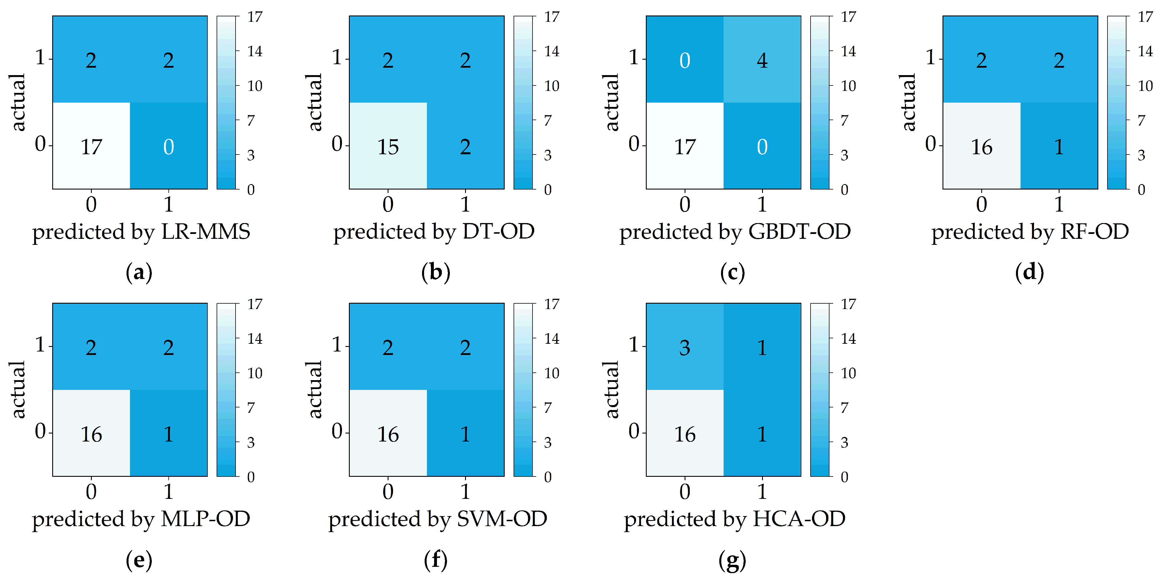
3.1. Performance of Machine Learning Models

The model performances are given in Figure 2. In detail, Figure 2a displays that the F1 score performed well for the LR, GBDT, and SVM models on the training set, all achieving an F1 score of 1. GBDT achieved an F1 score of 1 on the test set, while the highest scores for LR and SVM were only 0.67 and 0.57, respectively (Figure 2c). Figure 2b shows that LR, GBDT, and SVM achieved better results than the DT, RF, MLP, and hierarchical cluster analysis (HCA) models regarding the AUC scores for training. The best AUC results on the test set were GBDT (AUC = 1) > LR (AUC = 0.75) > SVM (AUC = 0.72) (Figure 2d). The results illustrated that GBDT has a certain degree of generalization performance. GBDT accurately identified groundwater TPH contamination in 82 gas stations in the training set and validated the algorithm’s capability in 21 gas stations in the test set. This can be attributed to the iterative residual correcting strategy of GBDT, which allowed GBDT to achieve better results than DT and RF [53]. LR performed poorly at dealing with unbalanced datasets, so the results were not satisfying [54]. In addition, SVM and MLP require high data density, which otherwise tends to underfit [55,56]. Moreover, the poor performance of the traditional HCA model compared to machine learning models may be attributed to the specificalities of feature variables. These feature variables were not the classical hydrochemical variables related to groundwater TPH, which is a significant difference from other studies where groundwater hydrochemical characteristics were used as input variables in the HCA model [57]. The input variables of the ML model are more flexible, which means all potentially relevant variables can be set as input variables, while the HCA method tends to use groundwater chemistry indicators as input variables. Moreover, the ML model has a stronger ability to find nonlinear relationships among variables than the HCA model. Overall, the GBDT model based on GridSearchCV achieved the highest F1 score and AUC in both the training and test sets. The prediction performance of GBDT was satisfying, while the other models were not.
Models trained with the data processed by SS tend to achieve better performance. In the LR, SVM, and MLP models, the best training results were achieved pre-processed by SS, with F1 scores and AUCs higher than those of OD and MMS. However, in the testing phase, the SS-built models did not necessarily achieve optimal results. The MMS-based LR model performed better in the testing phase, while the SVM was better using OD, indicating that overfitting occurred when using SS for training LR and SVM [58]. Furthermore, for the tree models, including DT, GBDT, and RF, the F1 scores and AUC results obtained from the three pre-processing methods were equal. It may be attributed to the operational mechanism of DT: each input feature variable is treated separately, and therefore each variable does not involve inconsistencies in the magnitudes of different feature variables [59]. Figure 3 shows the confusion matrix of the best-performing models on the test set. GBDT performed well on the 21 samples in the test set, correctly identifying all 4 TPH-contaminated sites (TP = 4, FP = 0, FN = 0). In comparison, other models could only identify one or two. This demonstrates the generalization ability of the GBDT model in identifying TPH contamination in groundwater from gas stations. Therefore, the GBDT model, pre-processed by OD, was chosen for further analysis.
Table 3 shows the information obtained for the GBDT model. Based on the boosting mechanism, GBDT classifies data by overlaying base learners, in which the residuals from the training process are continuously reduced [36]. In this study, the hyperparameter associated with boosting is n_estimators, which eventually took a value of 25, implying that 25 boosting stages were performed during the implementation. Among the hyperparameters related to the tree model, the optimal criterion was friedman_mse. Therefore, friedman_mse, a modified mean squared error function, was chosen to measure the impurities of the nodes [60]. Min_samples_split determines the minimum number of samples required for each internal node to be divided. The optimal value of min_samples_split was 0.1, which means that 10% of the training samples were required to split an internal node. Max_depth means that a single DT is limited in further subdividing the nodes, with an optimal value of three. The optimal value of min_samples_leaf was three, indicating the minimum number of samples in each tree leaf node. Min_samples_leaf is complementary to min_samples_split.

3.2. Model Optimization

Excessive training time is unacceptable due to the wide range of different site types, pollutants, and the fact that the training time of the model increases with the sample size. Table 4 presents the time the model’s training consumes based on the GridSearchCV method. MLP consumed the most time, followed by RF and GBDT. Overall, this was attributed to the exhaustive search mechanism of GridSearchCV. However, the single attempt time of MLP was only 1.21–1.28 s. This resulted from the fact that MLP had set the largest number of parameter groups (198,720). RF had the longest single attempt time (3.64 s), so its total time was much longer than GBDT. The GBDT model with the optimal predictive performance had the problem of inefficiency. The single attempt time was about 1.5 s, and the total was more than 5 h. The MLP algorithm set the largest number of parameter groups, since 230 different hidden layer sizes were designed. In addition, both RF and GBDT had a number of parameter groups of the order of 104. As a result, MLP, GBDT, and RF were time-consuming. For algorithms such as LR, GBDT, RF, and MLP, MMS or SS pre-processing of the input shortened the time to train the model. Nevertheless, the total training time for GBDT was still unacceptable.
Since GBDT can achieve optimal identification performance, the hyperparameters search process of GBDT was considered to be optimized to improve the efficiency of model training. Here, we proposed to optimize the model parameters by using BO. The settings of BO were as follows:
  • Black box function: the cross-validation score of the GBDT algorithm, and the metrics are F1 score and AUC.
  • Random search step: 5.
  • The number of iterations: 100.
  • Range of hyperparameters: see Table 5. The input of hyperparameters to BO can only be float instead of string and integer. Therefore, the criterion of GBDT is set to friedman_mse, which is also the default value of the model.
Table 6 displays the results of the hyperparameters optimized by BO. Compared to GridSearchCV, the optimal hyperparameters searched by BO differed from that of GridSearchCV. However, BO achieved the best performance on both the training and test sets, indicating that the hyperparameters optimized by BO can also exploit the best learning ability of GBDT [61]. Compared to GBDT, the training efficiency of BO-GBDT was much higher, taking only 1/37 of the total time of GBDT. In terms of the single attempt time, BO-GBDT took 5.13 s while GBDT spent 1.5 s for a single model, reflecting the value of BO-GBDT in improving overall efficiency. Therefore, the BO-GBDT model can improve the efficiency of identifying groundwater TPH contamination sites at gas stations without reducing the identification accuracy.

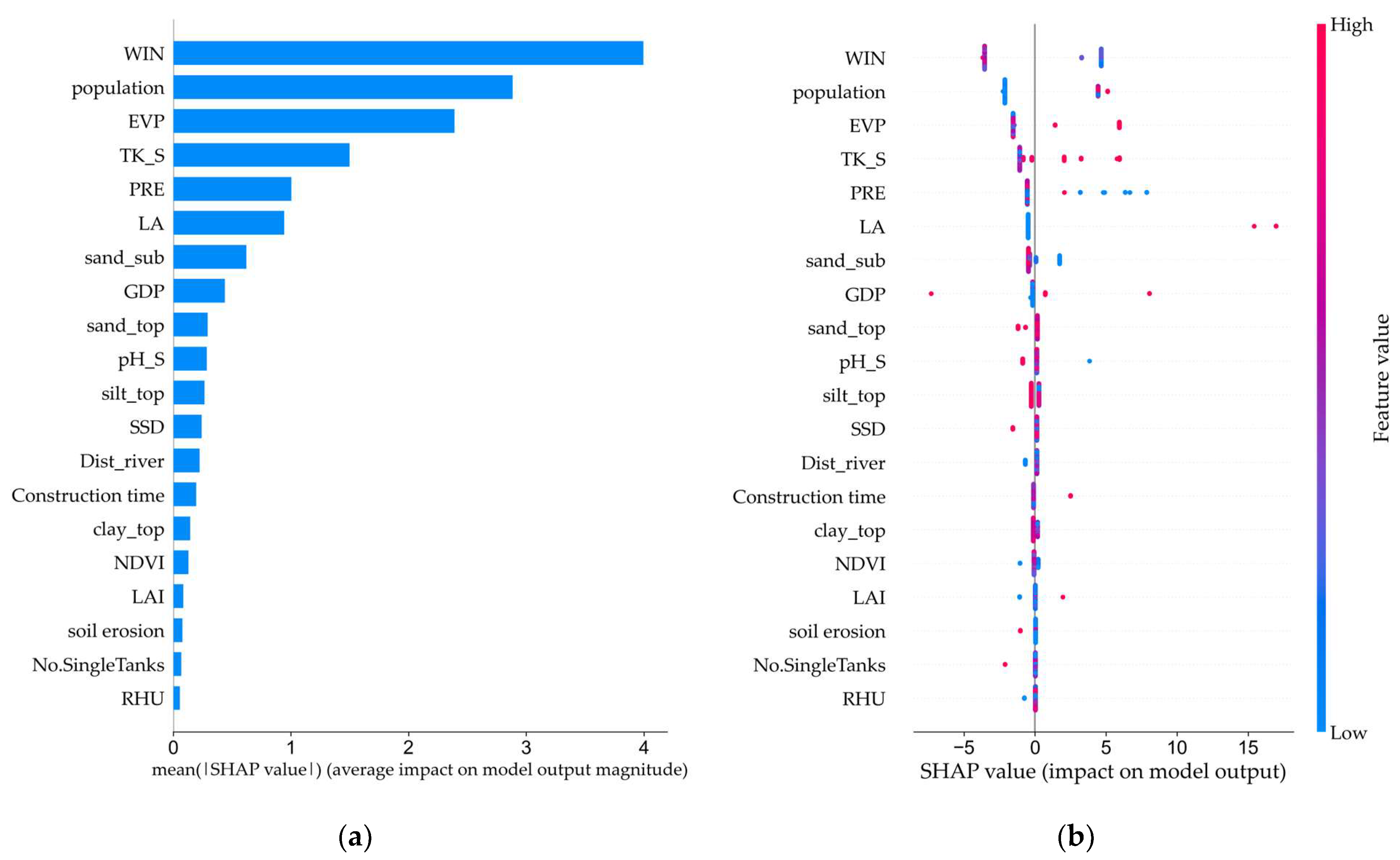
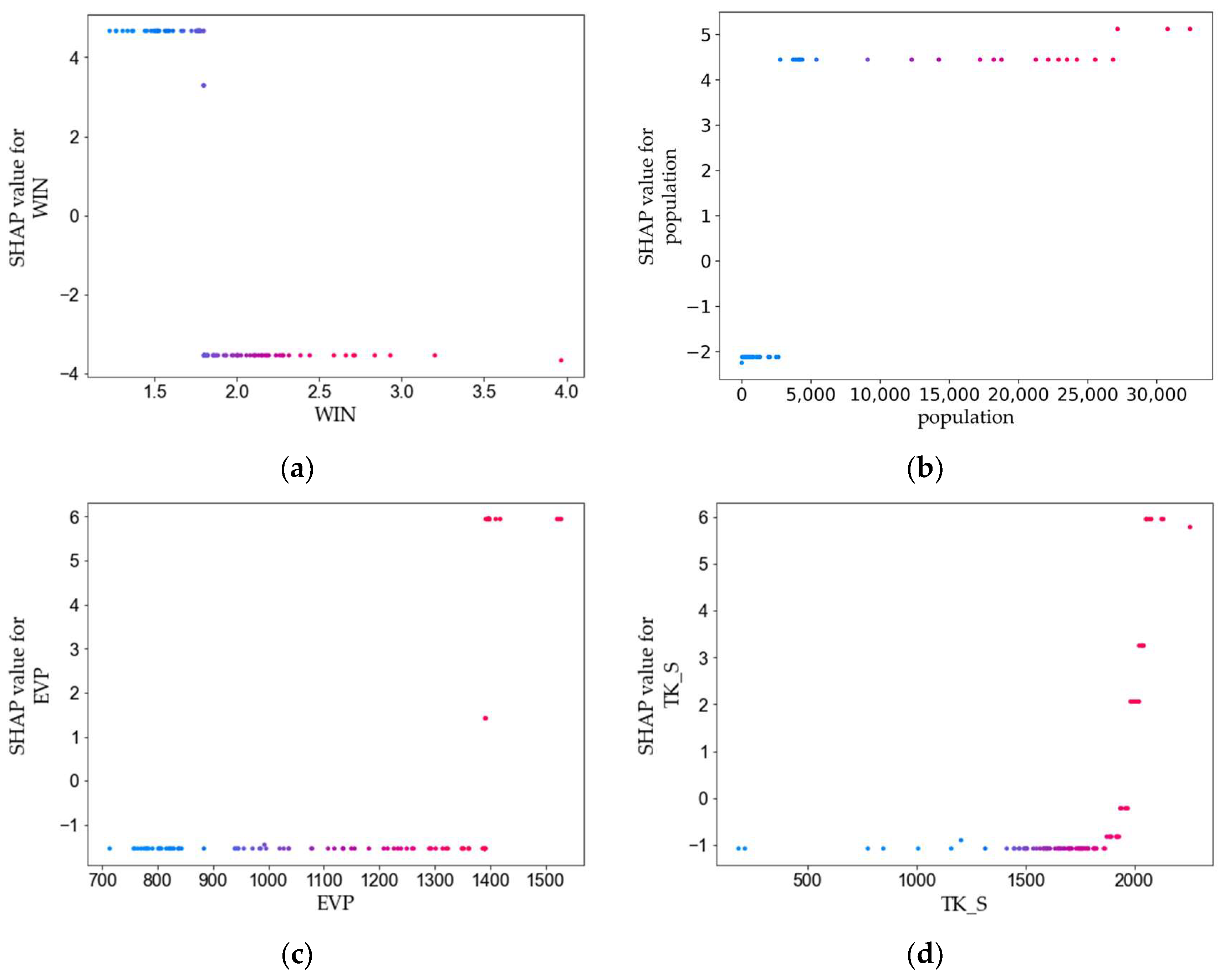
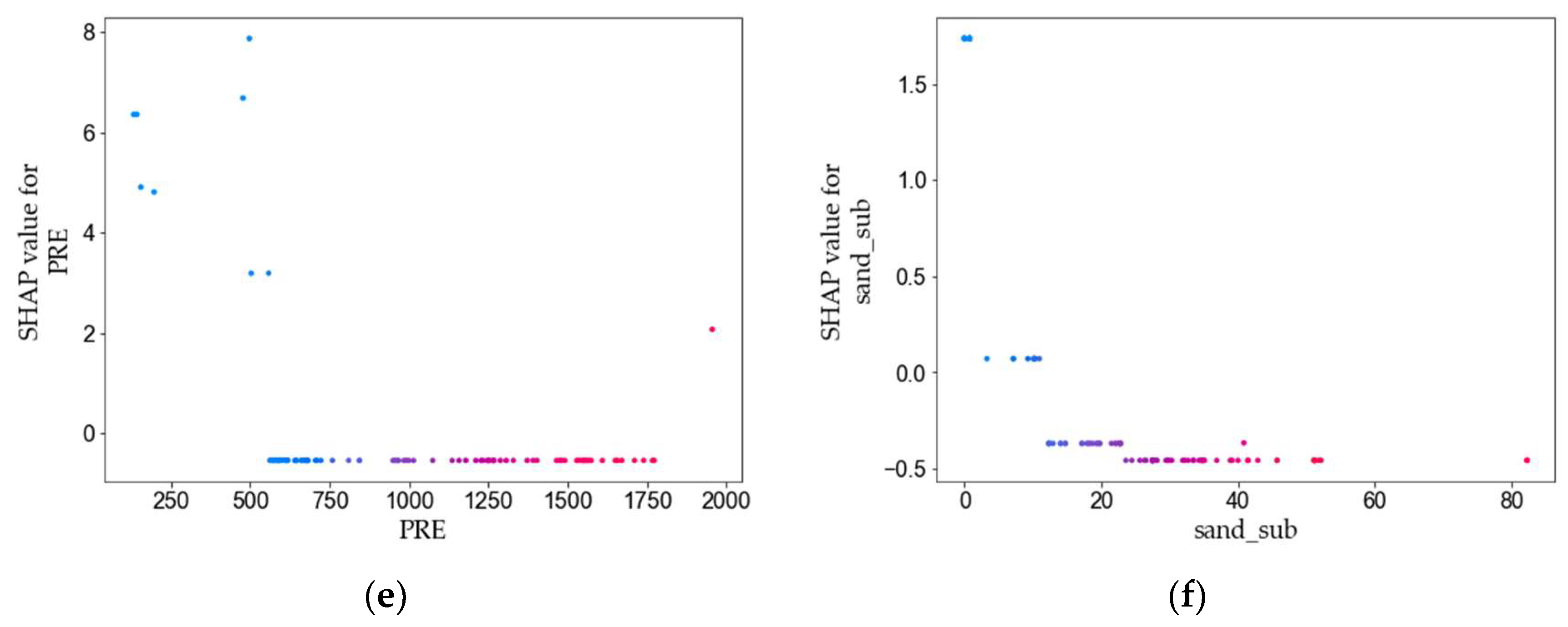
3.3. Feature Variables Analysis

The top 20 ranked feature variables were presented in the variable importance plot (Figure 4a), including WIN (wind), population, EVP (evaporation), TK_S (total potassium in the soil), PRE (precipitation), LA (leakage accidents), sand_sub (the content of sand in the subsoil), GDP, sand_top, pH_S, silt_top, SSD, Dist_river, construction time, clay_top, NDVI, LAI, soil erosion, NO.SingleTanks, RHU. WIN was regarded as the essential variable for identifying groundwater TPH contamination under gas stations in China (Figure 4a). The WIN distribution in the SHAP summary results further confirmed the high importance of wind speed in identifying groundwater TPH contamination at gas stations (Figure 4b). The results implied that wind speed lower than 1.8 m/s resulted in a higher probability of groundwater TPH contamination (Figure 5a). Part of the reason for this result may be the acceleration of the gasoline vaporization rate by increased surface wind speeds, which results in less TPH leaking into the groundwater [62]. Moreover, the natural attenuation of TPH could be enhanced by an active water cycle under strong wind [63]. The population showed high importance in identifying groundwater TPH contamination (Figure 4a). The SHAP value gradually increased with population, and meanwhile the positive effect on the probability of groundwater TPH contamination increased as well (Figure 4b). The SHAP value was positive when the population was more than 2780 p/km2 (Figure 5b), indicating that groundwater TPH contamination is more likely to occur at gas stations in densely populated areas, which may be related to the high volume of transportation and storage due to the high demand for gasoline [64]. The association between population and groundwater TPH contamination reflected the enormous impact of human activities on groundwater around gas stations, including TPH transportation, storage, and accidental spills. EVP, as another meteorological variable, was also important to the BO-GBDT model. The SHAP values were negative with lower EVP values (Figure 4b). Specifically, when the EVP was below 1391 mm/a, the groundwater at the gas station was not likely to be contaminated with TPH (Figure 5c). In contrast, the probability of groundwater TPH contamination increased remarkably when EVP was higher than 1391 mm/a, which could be ascribed to the increase in TPH concentration caused by water evaporation [65,66]. Moreover, high EVP may result from high permeability, which may accelerate the transport of TPH from soil to groundwater.
TK_S between 0 and 1969 mg/kg has a negative SHAP value, while it has a positive SHAP value when TK_S is greater than 1969 mg/kg (Figure 5d). This indicates that the high TK_S is somewhat related to the TPH pollution of groundwater in the local gas station. In addition, PRE was identified as another important variable associated with groundwater TPH contamination. The results of the SHAP summary showed that the decrease in PRE increased the probability of groundwater TPH contamination (Figure 4b). The SHAP values start to turn negative when the PRE exceeds 560 (Figure 5e). This result may be related to the high natural attenuation of TPH at high value of PRE [67]. Meanwhile, PRE tends to be negatively correlated with TK_S due to the strong leaching effect caused by rainfall [68], which explains the positive correlation between TK_S and SHAP value. LA was also identified as a significant variable. Groundwater TPH contamination occurred at all gas stations where tank leaks have been detected (Figure 4b), indicating that once tank leaks occur, groundwater is likely to be contaminated. The results alert the environmental authorities to monitor the gas storage tanks more closely to avoid the risk of LA. The SHAP value increased with a decrease in sand_sub, indicating that TPH contamination of groundwater at gas stations is more likely to occur with low sub-soil sand content. The SHAP value was negative when sand_sub was between 0 and 12.33% (Figure 5f). This may be related to the TPH trapping effect of the sand in the subsoil [69]. For features ranked after sand_sub, their SHAPs are concentrated around 0, indicating that they play a minor role in the well-established model (Figure 4).
Furthermore, the above seven crucial feature variables were set as inputs of BO-GBDT to investigate their identification performance of groundwater TPH pollution. The settings of the input variables are shown in Table 7.
The performance metrics of the BO-GBDT model obtained by training with the seven input settings are shown in Figure 6. Overall, the F1 score and AUC of the BO-GBDT model showed an increasing trend when the number of input variables was increased, showing the boosting effect of increasing variables on the model performance. It is worth noting that the model already performed well when using only WIN as an input variable, with F1 scores and AUCs of 0.87 and 0.90 on the training set and 0.75 and 0.85 on the test set, respectively, reflecting the vital role of WIN in the model’s prediction. This is in agreement with the findings presented in Figure 3a. At five variables, the predictive performance slightly decreases compared to four, suggesting that with few feature variables, adding features may potentially introduce overfitting, as previously reported [70]. The model’s performance saw a notable improvement when using six input variables (training F1 score = 1, test F1 score = 0.89, training AUC = 1, test AUC = 0.97). When the number of input features was seven, the results were consistent with those when the number of features was six. It was found that when using six or seven input variables, all the prediction errors involved cases where no contamination was predicted as contamination (n = 1). In that case, although the model’s results are not perfect, they are relatively conservative. Therefore, a reliable model for identifying groundwater TPH contamination can be established using only six variables (WIN, population, EVP, TK_S, PRE, LA).
The variables analysis results reveal that TPH contamination in groundwater at gas stations in China is a combination of natural and anthropogenic factors. China’s eco-environmental authorities are undertaking a series of pollution prevention control of gas stations, as required by policy documents such as the National Groundwater Pollution Prevention and Control Plan (2011–2020) and the 14th Five-Year Plan for Soil, Groundwater and Rural Ecological Protection. The human activities at gas stations including the transportation and storage of gas need to be further regulated. We recommend that managers pay more attention to the supervision of gas storage tanks in densely populated areas in order to detect potential leaks on time. This study also provides a scientific basis for the site selection of new gas stations. From the point of view of avoiding groundwater contamination by TPH, areas with low wind speed, low evaporation, low population density, and high precipitation are considered suitable sites for new gas stations.

4. Conclusions

This study applied a machine learning approach to develop models to identify groundwater contamination sites. An evaluation of model prediction performance and efficiency was carried out. A case study was conducted using gas station sites in China with groundwater TPH as the target contaminant. The model developed by the GBDT algorithm had the most satisfying prediction performance (F1 score = 1, AUC = 1). Compared to GridsearchCV, the BO-GBDT model could significantly improve the modeling efficiency without degrading the prediction performance, with a time from 19,125 s to 513 s. Therefore, BO-GBDT was the most reliable prediction model in this study. The SHAP results displayed that the critical feature variables in the BO-GBDT model included wind, population, evaporation, total potassium in the soil, precipitation, and leakage accident.
It can be seen that the machine learning approach, particularly being optimized with BO, shows potential for identifying groundwater contamination sites. The limitations of the method mainly come from two aspects: (1) the machine learning model has inherent uncertainty itself, which may affect the generalization ability; (2) the relatively small sample size introduces uncertainty into the results of this study. In future studies, researchers should incorporate more gas station contamination samples for further model improvement and validation. Moreover, detailed experiments should be conducted to further verify the relationships between the variables and TPH contamination identified in this study. In addition, some other machine learning models, such as deep learning-based models, also deserve to be studied for groundwater contamination site identification. The idea of using a machine learning approach to identify groundwater contamination sites is highly suggested to be employed in more countries/regions and more types of sites and contaminants.

Author Contributions

Conceptualization, Y.H. and Q.H.; methodology, Y.H. and G.L.; validation, W.L.; investigation, H.N., G.L. and S.L.; writing—original draft preparation, Y.H. and L.D.; writing—review and editing, M.Y. and Q.H.; visualization, Y.H. and M.Y.; supervision, Q.H.; funding acquisition, L.D. and W.L. All authors have read and agreed to the published version of the manuscript.

Funding

This research was funded by the National Key R&D Program of China (Grant NO. 2019YFC1803900 and NO. 2018YFC1800204).

Data Availability Statement

The datasets generated during the current study are available from the first author on reasonable request.

Acknowledgments

Acknowledgement for the data support from National Cryosphere Desert Data Center. (http://www.ncdc.ac.cn (accessed on 23 August 2022)), National Earth System Science Data Center, National Science & Technology Infrastructure of China (http://www.geodata.cn (accessed on 23 August 2022)).

Conflicts of Interest

The authors declare no conflict of interest.

References

  1. Jiang, Y.; Huang, M.; Chen, X.; Wang, Z.; Xiao, L.; Xu, K.; Zhang, S.; Wang, M.; Xu, Z.; Shi, Z. Identification and risk prediction of potentially contaminated sites in the Yangtze River Delta. Sci. Total Environ. 2022, 815, 151982. [Google Scholar] [CrossRef] [PubMed]
  2. Hou, D. Ten grand challenges for groundwater pollution prevention and remediation at contaminated sites in China. Res. Environ. Sci. 2022, 35, 2015–2025. [Google Scholar]
  3. Li, H.; Gu, J.; Hanif, A.; Dhanasekar, A.; Carlson, K. Quantitative decision making for a groundwater monitoring and subsurface contamination early warning network. Sci. Total Environ. 2019, 683, 498–507. [Google Scholar] [CrossRef]
  4. Van Liedekerke, M.; Prokop, G.; Rabl-Berger, S.; Kibblewhite, M.; Louwagie, G. Progress in the Management of Contaminated Sites in Europe; European Commission: Brussels, Belgium, 2014. [Google Scholar]
  5. Jiang, Y.; Wang, H.; Lei, M.; Hou, D.; Chen, S.; Hu, B.; Huang, M.; Song, W.; Shi, Z. An integrated assessment methodology for management of potentially contaminated sites based on public data. Sci. Total Environ. 2021, 783, 146913. [Google Scholar] [CrossRef] [PubMed]
  6. Rampanelli, G.B.; Braun, A.B.; Visentin, C.; Trentin, A.W.d.S.; da Cruz, R.; Thomé, A. The process of selecting a method for identifying potentially contaminated sites—A case study in a municipality in southern Brazil. Water Air Soil Pollut. 2021, 232, 26. [Google Scholar] [CrossRef]
  7. Pitsaki, K.; Boura, F.; Pantazidou, M.; Katsiri, A. Methodologies for compiling national inventories of contaminated sites and conducting preliminary site screening. Glob. Nest J. 2014, 16, 24–35. [Google Scholar] [CrossRef]
  8. Rouillon, M.; Taylor, M.P.; Dong, C.Y. Reducing risk and increasing confidence of decision making at a lower cost: In-situ pXRF assessment of metal-contaminated sites. Environ. Pollut. 2017, 229, 780–789. [Google Scholar] [CrossRef]
  9. Wiséen, T.; Wester-Herber, M. Dirty soil and clean consciences: Examining communication of contaminated soil. Water Air Soil Pollut. 2007, 181, 173–182. [Google Scholar] [CrossRef]
  10. Sjöberg, L. The allegedly simple structure of experts’ risk perception: An urban legend in risk research. Sci. Technol. Hum. Values 2002, 27, 443–459. [Google Scholar] [CrossRef]
  11. Wester-Herber, M.; Warg, L.-E. Did they get it? Examining the goals of risk communication within the Seveso II Directive in a Swedish context. J. Risk Res. 2004, 7, 495–506. [Google Scholar] [CrossRef]
  12. Jordan, M.I.; Mitchell, T.M. Machine learning: Trends, perspectives, and prospects. Science 2015, 349, 255–260. [Google Scholar] [CrossRef] [PubMed]
  13. Rizeei, H.M.; Azeez, O.S.; Pradhan, B.; Khamees, H.H. Assessment of groundwater nitrate contamination hazard in a semi-arid region by using integrated parametric IPNOA and data-driven logistic regression models. Environ. Monit. Assess. 2018, 190, 633. [Google Scholar] [CrossRef] [PubMed]
  14. Saghebian, S.M.; Sattari, M.T.; Mirabbasi, R.; Pal, M. Ground water quality classification by decision tree method in Ardebil region, Iran. Arab. J. Geosci. 2013, 7, 4767–4777. [Google Scholar] [CrossRef]
  15. Erickson, M.L.; Elliott, S.M.; Brown, C.J.; Stackelberg, P.E.; Ransom, K.M.; Reddy, J.E.; Cravotta, C.A., III. Machine-Learning predictions of high arsenic and high manganese at drinking water depths of the glacial aquifer system, northern continental United States. Environ. Sci. Technol. 2021, 55, 5791–5805. [Google Scholar] [CrossRef] [PubMed]
  16. Nafouanti, M.B.; Li, J.; Mustapha, N.A.; Uwamungu, P.; Al-Alimi, D. Prediction on the fluoride contamination in groundwater at the Datong Basin, Northern China: Comparison of random forest, logistic regression and artificial neural network. Appl. Geochem. 2021, 132, 105054. [Google Scholar] [CrossRef]
  17. Jafari, R.; Torabian, A.; Ghorbani, M.A.; Mirbagheri, S.A.; Hassani, A.H. Prediction of groundwater quality parameter in the Tabriz plain, Iran using soft computing methods. J. Water Supply Res. Technol.-Aqua 2019, 68, 573–584. [Google Scholar] [CrossRef]
  18. Mao, H.R.; Wang, C.Y.; Qu, S.; Liao, F.; Wang, G.C.; Shi, Z.M. Source and evolution of sulfate in the multi-layer groundwater system in an abandoned mine-Insight from stable isotopes and Bayesian isotope mixing model. Sci. Total Environ. 2023, 859, 12. [Google Scholar] [CrossRef]
  19. An, Y.; Zhang, Y.; Yan, X. An integrated Bayesian and machine learning approach application to identification of groundwater contamination source parameters. Water 2022, 14, 2447. [Google Scholar] [CrossRef]
  20. Li, J.; Lu, W.; Luo, J. Groundwater contamination sources identification based on the Long-Short Term Memory network. J. Hydrol. 2021, 601, 126670. [Google Scholar] [CrossRef]
  21. Wu, Q.; Zhang, X.; Zhang, Q. Current situation and control measures of groundwater pollution in gas station. In Proceedings of the 2017 3rd International Conference on Energy, Environment and Materials Science (EEMS), Northwestern Polytechnical University, Singapore, 28–30 July 2017. [Google Scholar]
  22. Rosales, R.M.; Martínez-Pagán, P.; Faz, A.; Bech, J. Study of subsoil in former petrol stations in SE of Spain: Physicochemical characterization and hydrocarbon contamination assessment. J. Geochem. Explor. 2014, 147, 306–320. [Google Scholar] [CrossRef]
  23. Yang, Q.; Chen, X.; Sun, C.; Kang, L.; Zhao, Z.; Chen, M. Spatial distribution of typical pollutants of gas stations in shallow water-table areas. Chin. J. Environ. Eng. 2014, 8, 98–103. [Google Scholar]
  24. Tiburtius, E.R.L.; Peralta-Zamora, P.; Emmel, A. Treatment of gasoline-contaminated waters by advanced oxidation processes. J. Hazard. Mater. 2005, 126, 86–90. [Google Scholar] [CrossRef]
  25. Zhao, L.; Deng, Y.; Huang, X.; Sun, Q. Problems and countermeasures of soil and groundwater environmental management in gas station. Adm. Tech. Environ. Monit. 2019, 31, 4–7. [Google Scholar]
  26. Lesage, S.; Xu, H.; Novakowski, K.S. Distinguishing natural hydrocarbons from anthropogenic contamination in ground water. Groundwater 1997, 35, 149–160. [Google Scholar] [CrossRef]
  27. GB 5749-2006; Standards for Drinking Water Quality. Ministry of Health of the People’s Republic of China; Standardization Administration of China: Beijing, China, 2006.
  28. HJ 164-2004; Technical Specification for Environmental Monitoring of Groundwater. State Environmental Protection Administration of the People’s Republic of China: Beijing, China, 2004.
  29. HJ 894-2017; Water Quality-Determination of Extractable Petroleum Hydro-Carbons (C10-C40)-Gas Chro-Matography. Ministry of Environmental Protection of the People’s Republic of China: Beijing, China, 2017.
  30. Mojaddadi, H.; Pradhan, B.; Nampak, H.; Ahmad, N.; Ghazali, A.H.b. Ensemble machine-learning-based geospatial approach for flood risk assessment using multi-sensor remote-sensing data and GIS. Geomat. Nat. Hazards Risk 2017, 8, 1080–1102. [Google Scholar] [CrossRef] [Green Version]
  31. McManus, S.L.; Richards, K.G.; Grant, J.; Mannix, A.; Coxon, C.E. Pesticide occurrence in groundwater and the physical characteristics in association with these detections in Ireland. Environ. Monit. Assess. 2014, 186, 7819–7836. [Google Scholar] [CrossRef]
  32. Wu, R.; Podgorski, J.; Berg, M.; Polya, D.A. Geostatistical model of the spatial distribution of arsenic in groundwaters in Gujarat State, India. Environ. Geochem. Health 2021, 43, 2649–2664. [Google Scholar] [CrossRef] [PubMed]
  33. Hinkle, S.R.; Tesoriero, A.J. Nitrogen speciation and trends, and prediction of denitrification extent, in shallow US groundwater. J. Hydrol. 2014, 509, 343–353. [Google Scholar] [CrossRef]
  34. Barad, S.; Mishra, P.; Sahu, P.C.; Sarkar, T.; Amin, M.F.M.; Choudhury, T.; Edinur, H.A.; Kari, Z.A.; Nandi, D.; Pati, S. Comparative approach of decision tree and CWQI analysis for classification of groundwater with a special reference to fluoride ion in drought-prone Boudh district of Odisha, India. Sustain. Water Resour. Manag. 2021, 7, 94. [Google Scholar] [CrossRef]
  35. Taherdangkoo, R.; Liu, Q.; Xing, Y.; Yang, H.; Cao, V.; Sauter, M.; Butscher, C. Predicting methane solubility in water and seawater by machine learning algorithms: Application to methane transport modeling. J. Contam. Hydrol. 2021, 242, 103844. [Google Scholar] [CrossRef]
  36. Naghibi, S.A.; Pourghasemi, H.R.; Dixon, B. GIS-based groundwater potential mapping using boosted regression tree, classification and regression tree, and random forest machine learning models in Iran. Environ. Monit. Assess. 2016, 188, 44. [Google Scholar] [CrossRef] [PubMed]
  37. Band, S.S.; Janizadeh, S.; Pal, S.C.; Chowdhuri, I.; Siabi, Z.; Norouzi, A.; Melesse, A.M.; Shokri, M.; Mosavi, A. Comparative analysis of artificial intelligence models for accurate estimation of groundwater nitrate concentration. Sensors 2020, 20, 5763. [Google Scholar] [CrossRef] [PubMed]
  38. Elith, J.; Leathwick, J.R.; Hastie, T. A working guide to boosted regression trees. J. Anim. Ecol. 2008, 77, 802–813. [Google Scholar] [CrossRef]
  39. Rajaee, T.; Ebrahimi, H.; Nourani, V. A review of the artificial intelligence methods in groundwater level modeling. J. Hydrol. 2019, 572, 336–351. [Google Scholar] [CrossRef]
  40. Ali, E.B.; Abdeslam, T.; Youssef, B. Groundwater quality forecasting using machine learning algorithms for irrigation purposes. Agric. Water Manag. 2021, 245, 106625. [Google Scholar] [CrossRef]
  41. Mosavi, A.; Sajedi Hosseini, F.; Choubin, B.; Taromideh, F.; Ghodsi, M.; Nazari, B.; Dineva, A.A. Susceptibility mapping of groundwater salinity using machine learning models. Environ. Sci. Pollut. Res. Int. 2020, 28, 10804–10817. [Google Scholar] [CrossRef]
  42. Jiang, X.; Xu, C. Deep learning and machine learning with Grid search to predict later occurrence of breast cancer metastasis using clinical data. J. Clin. Med. 2022, 11, 5772. [Google Scholar] [CrossRef]
  43. Shamsuddin, I.I.S.; Othman, Z.; Sani, N.S. Water quality index classification based on machine learning: A case from the Langat River Basin model. Water 2022, 14, 2939. [Google Scholar] [CrossRef]
  44. Im, G.; Lee, D.; Lee, S.; Lee, J.; Lee, S.; Park, J.; Heo, T.-Y. Estimating chlorophyll-a concentration from hyperspectral data using various machine learning techniques: A case study at Paldang Dam, South Korea. Water 2022, 14, 4080. [Google Scholar] [CrossRef]
  45. Wong, J.; Manderson, T.; Abrahamowicz, M.; Buckeridge, D.L.; Tamblyn, R. Can hyperparameter tuning improve the performance of a super learner?: A case study. Epidemiology 2019, 30, 521–531. [Google Scholar] [CrossRef]
  46. Pannakkong, W.; Harncharnchai, T.; Buddhakulsomsiri, J. Forecasting daily electricity consumption in Thailand using regression, artificial neural network, support vector machine, and hybrid Models. Energies 2022, 15, 3105. [Google Scholar] [CrossRef]
  47. Garrido-Merchán, E.C.; Hernández-Lobato, D. Dealing with categorical and integer-valued variables in Bayesian Optimization with Gaussian processes. Neurocomputing 2020, 380, 20–35. [Google Scholar] [CrossRef] [Green Version]
  48. Yan, M.; Shen, Y. Traffic accident severity prediction based on random forest. Sustainability 2022, 14, 1729. [Google Scholar] [CrossRef]
  49. Wang, Y.; Kandeal, A.W.; Swidan, A.; Sharshir, S.W.; Abdelaziz, G.B.; Halim, M.A.; Kabeel, A.E.; Yang, N. Prediction of tubular solar still performance by machine learning integrated with Bayesian optimization algorithm. Appl. Therm. Eng. 2021, 184, 116233. [Google Scholar] [CrossRef]
  50. Lundberg, S.M.; Lee, S.-I. A unified approach to interpreting model predictions. In Proceedings of the the 31st International Conference on Neural Information Processing Systems, Long Beach, CA, USA, 4–9 December 2017. [Google Scholar]
  51. Vega García, M.; Aznarte, J.L. Shapley additive explanations for NO2 forecasting. Ecol. Inform. 2020, 56, 101039. [Google Scholar] [CrossRef]
  52. Fryer, D.; Strümke, I.; Nguyen, H. Shapley values for feature selection: The good, the bad, and the axioms. IEEE Access 2021, 9, 144352–144360. [Google Scholar] [CrossRef]
  53. Shen, Z.; Yong, B. Downscaling the GPM-based satellite precipitation retrievals using gradient boosting decision tree approach over Mainland China. J. Hydrol. 2021, 602, 126803. [Google Scholar] [CrossRef]
  54. Song, Y.; Niu, R.; Xu, S.; Ye, R.; Peng, L.; Guo, T.; Li, S.; Chen, T. Landslide susceptibility mapping based on weighted gradient boosting decision tree in Wanzhou section of the Three Gorges Reservoir area (China). ISPRS Int. J. Geo-Inf. 2019, 8, 4. [Google Scholar] [CrossRef] [Green Version]
  55. Park, Y.; Ligaray, M.; Kim, Y.M.; Kim, J.H.; Cho, K.H.; Sthiannopkao, S. Development of enhanced groundwater arsenic prediction model using machine learning approaches in Southeast Asian countries. Desalination Water Treat. 2015, 57, 12227–12236. [Google Scholar] [CrossRef]
  56. Purkait, B. Application of artificial neural network model to study arsenic contamination in groundwater of Malda District, eastern India. J. Environ. Inform. 2008, 12, 140–149. [Google Scholar] [CrossRef] [Green Version]
  57. Bi, P.; Pei, L.; Huang, G.; Han, D.; Song, J. Identification of groundwater contamination in a rapidly urbanized area on a regional scale: A new approach of multi-hydrochemical evidences. Int. J. Environ. Res. Public Health 2021, 18, 12143. [Google Scholar] [CrossRef]
  58. Han, H.; Jiang, X. Overcome support vector machine diagnosis overfitting. Cancer Inform. 2014, 13, 145–158. [Google Scholar] [CrossRef] [PubMed]
  59. Krzywinski, M.; Altman, N. Classification and regression trees. Nat. Methods 2017, 14, 757–758. [Google Scholar] [CrossRef]
  60. Friedman, J.H. Greedy function approximation: A gradient boosting machine. Ann. Stat. 2001, 29, 1189–1232. [Google Scholar] [CrossRef]
  61. Rong, G.; Alu, S.; Li, K.; Su, Y.; Zhang, J.; Zhang, Y.; Li, T. Rainfall induced landslide susceptibility mapping based on Bayesian optimized random forest and gradient boosting decision tree models—A case study of Shuicheng County, China. Water 2020, 12, 3066. [Google Scholar] [CrossRef]
  62. Halmemies, S.; Gröndahl, S.; Nenonen, K.; Tuhkanen, T. Estimation of the time periods and processes for penetration of selected spilled oils and fuels in different soils in the laboratory. Spill Sci. Technol. Bull. 2003, 8, 451–465. [Google Scholar] [CrossRef]
  63. Maxwell, R.M.; Chow, F.K.; Kollet, S.J. The groundwater–land-surface–atmosphere connection: Soil moisture effects on the atmospheric boundary layer in fully-coupled simulations. Adv. Water Resour. 2007, 30, 2447–2466. [Google Scholar] [CrossRef] [Green Version]
  64. Vandana; Priyadarshanee, M.; Mahto, U.; Das, S. Chapter 2-Mechanism of toxicity and adverse health effects of environmental pollutants. In Microbial Biodegradation and Bioremediation, 2nd ed.; Das, S., Dash, H.R., Eds.; Elsevier: Amsterdam, The Netherlands, 2022; pp. 33–53. [Google Scholar]
  65. Sun, H.; Yang, X.; Xie, J.; Li, X.; Zhao, Y. Remediation of diesel-contaminated aquifers using thermal conductive heating coupled with thermally activated persulfate. Water Air Soil Pollut. 2021, 232, 293. [Google Scholar] [CrossRef]
  66. Falciglia, P.P.; Maddalena, R.; Mancuso, G.; Messina, V.; Vagliasindi, F.G.A. Lab-scale investigation on remediation of diesel-contaminated aquifer using microwave energy. J. Environ. Manag. 2016, 167, 196–205. [Google Scholar] [CrossRef] [Green Version]
  67. McAlexander, B.; Sihota, N. Influence of ambient temperature, precipitation, and groundwater level on natural source zone depletion rates at a large semiarid LNAPL site. Groundw. Monit. Remediat. 2019, 39, 54–65. [Google Scholar] [CrossRef] [Green Version]
  68. Ma, J. The influence of rainstorm on soil components and properties:a case study of Biyang rainstorm area, Henan province. Geogr. Res. 2004, 23, 55–62. [Google Scholar]
  69. Zhang, S.; Su, X.; Lin, X.; Zhang, Y.; Zhang, Y. Experimental study on the multi-media PRB reactor for the remediation of petroleum-contaminated groundwater. Environ. Earth Sci. 2015, 73, 5611–5618. [Google Scholar] [CrossRef]
  70. Isazadeh, M.; Biazar, S.M.; Ashrafzadeh, A. Support vector machines and feed-forward neural networks for spatial modeling of groundwater qualitative parameters. Environ. Earth Sci. 2017, 76, 610. [Google Scholar] [CrossRef]
Figure 1. Methodological framework in this study.
Water 15 01326 g001
Figure 2. Performance evaluation of all machine learning models. (a) F1 score and (b) AUC of the model on the training set; (c) F1 score and (d) AUC of the model on the test set.
Water 15 01326 g002
Figure 3. The confusion matrix of the best-performing models on the test set. In each subgraph, from top left to bottom right are FN, TP, TN, FP. (a) LR-MMS; (b) DT-OD; (c) GBDT-OD; (d) RF-OD; (e) MLP-OD; (f) SVM-OD; (g) HCA-OD.
Water 15 01326 g003
Figure 4. Results of SHAP analysis of the BO-GBDT model. (a) Bar diagram showing the feature variable importance.; (b) SHAP summary plot of feature variables.
Water 15 01326 g004
Figure 5. Scatter plots of feature variables and SHAP values. (a) WIN; (b) population; (c) EVP; (d) TK_S; (e) PRE; (f) sand_sub.
Water 15 01326 g005aWater 15 01326 g005b
Figure 6. Performance of BO-GBDT model established by different input settings on the training and test sets.
Water 15 01326 g006
Table 1. Description of feature variables in this study.
CategoryVariableDescriptionType
Management variablesKILKey investigation list. Whether the station is on the key investigation list or notcategorical
OCOperating condition. Whether the station is open for businesscategorical
OwnerThe owner of the gas stationcategorical
LALeakage accident. Whether the station has ever had oil leakage accidentscategorical
GWPAGroundwater protection area. Whether the station is located in a groundwater protection areacategorical
Gas station variablesConstruction TimeThe length of time since the station was constructeddiscrete
No.TanksTotal number of tanks at the gas stationdiscrete
No.SingleTanksTotal number of single-layer tanks at the gas stationdiscrete
Impermeable pondsWhether the gas station has built impermeable pondscategorical
PipelineType of pipeline at the stationcategorical
Geography and remote sensing variablesDist_lakeThe distance from the nearest lakecontinuous
Dist_riverThe distance from the nearest rivercontinuous
ElevationThe elevation where the gas station is locatedcontinuous
NPPNet primary productivity at the location of the gas stationcontinuous
LAILeaf area index. The leaf area index of the location of the gas stationcontinuous
LanduseLand use types around gas stationscategorical
NDVINormalized vegetation index of the gas station locationcontinuous
Social economy variablesNLINight light index. The night light index of the gas station locationcontinuous
populationThe population of the town where the gas station is locatedcontinuous
GDPTotal GDP of the cell grid where the gas station is locatedcontinuous
Meteorological variablesPermafrost typeThe type of frozen soilcategorical
EVPAnnual mean evaporationcontinuous
GSTAnnual mean ground surface temperaturecontinuous
PREAnnual precipitation continuous
PRSAnnual mean pressurecontinuous
RHUAnnual mean relative humiditycontinuous
SSDAnnual sunshinecontinuous
TEMAnnual mean temperaturecontinuous
WINAnnual mean wind speedcontinuous
Soil variablesSoil erosionTypes and properties of external forces of soil erosioncategorical
clay_topThe proportion of clay in the topsoil (0–30 cm)continuous
sand_topThe proportion of sand in the topsoil continuous
silt_topThe proportion of silt in the topsoil continuous
soil moistureThe moisture of the topsoilcontinuous
clay_subThe content of clay in the subsoil (30–100 cm)continuous
sand_subThe content of sand in the subsoilcontinuous
CEC_SSoil cation exchange capacity in 100–200 cmcontinuous
TK_STotal potassium in soil from 15 to 30 cmcontinuous
gravel_SGravel content in soil from 30 to 60 cmcontinuous
pH_SSoil pH in the range of 30–60 cmcontinuous
Table 2. Hyperparameter settings [42,43,44,45,46].
AlgorithmHyperparameterDescriptionRange
LRCRegularization parameter. A smaller C means that the model may have better generalization, but it is also more likely to underfit[0.0001, 0.001, 0.01, 0.1, 1, 10, 100, 1000, 10,000]
DTcriterionSelects the criteria by which attributes will be selected for separation[gini, entropy, log_loss]
min_samples_leafThe minimum number of samples required at a leaf node[1, 2, 3, 4, 5, 6, 7, 8, 9, 10]
max_depthThe maximum depth of the tree[3, 4, 5, 6]
min_samples_splitThe minimum number of samples required to split internal nodes[0.1, 0.2, 0.3, 0.4, 0.6, 0.8, 1.2]
GBDTcriterionSelects the criteria by which attributes will be selected for separation[friedman_mse, squared_error]
n_estimatorsThe number of boosting stages to perform. It is represented in GBDT as the number of decision trees[10, 25, 50, 60, 70, 80, 90, 100, 110, 120, 130, 140, 150, 160, 170, 180, 190, 200, 500, 1000, 1500, 2000]
DT hyperparametersmin_samples_leaf, max_depth, and min_samples_splitSame as DT
RFn_estimatorsThe number of trees in the random forestSame as GBDT
DT hyperparametersCriterion, min_samples_leaf, max_depth, and min_samples_splitSame as DT
MLPhidden_layer_sizesThe number of hidden layers in the neural network and the number of neurons in each hidden layer[‘layer1’: 1 to 20 (n), ‘layer2’: 0 to n]
activationActivation function for the hidden layer[identity, logistic, tanh, relu]
max_iterThe maximum number of iterations of the solver[100, 280, 460, 640, 820, 1000]
learning_rate_initThe initial learning rate used. It controls the step size when the weight is updated[0.001, 0.0108, 0.0206, 0.0304, 0.0402, 0.05]
momentumMomentum for gradient descent update[0.5, 0.58, 0.66, 0.74, 0.82, 0.9]
SVMCRegularization parameter[0.001, 0.01, 0.1, 1, 10, 100, 3300, 1000]
kernelSpecifies the kernel type used in the algorithm[linear, rbf, poly, sigmoid]
Table 3. Information on the GBDT model for groundwater TPH contamination identification.
AlgorithmPre-ProcessingHyperparameterParameter Optimum
GBDTODcriterionfriedman_mse
n_estimators25
min_samples_leaf3
max_depth3
min_samples_split0.1
Table 4. Time consumption summary of training models based on the GridSearchCV method.
AlgorithmPre-ProcessingNumber of Parameter GroupsTotal Time (s)Single Attempt Time (s)
LROD953.105.90
MMS913.101.46
SS97.750.86
DTOD84060.570.07
MMS84060.070.07
SS84070.700.08
GBDTOD12,32019,1251.55
MMS12,32018,6651.52
SS12,32018,9611.54
RFOD18,48067,2833.64
MMS18,48066,5743.60
SS18,48065,3263.53
MLPOD198,720253,5001.28
MMS198,720248,4001.25
SS198,720240,7801.21
SVMOD322.240.07
MMS323.950.12
SS323.020.09
Table 5. Hyperparameter range for BO-GBDT.
HyperparameterRange
n_estimators(1, 2000)
min_samples_leaf(1, 10)
max_depth(3, 6)
min_samples_split(0.1, 1)
Table 6. The BO results in the GBDT model.
HyperparameterHyperparameter
Optimum
PerformanceTraining Time
n_estimators978Training: F1 score = 1, AUC = 1
Test: F1 score = 1, AUC = 1
513 s
min_samples_leaf1
max_depth3
min_samples_split0.9745
Table 7. Input combinations for each BO-GBDT model.
Number of VariablesInput Variables
1WIN
2WIN, population
3WIN, population, EVP
4WIN, population, EVP, TK_S
5WIN, population, EVP, TK_S, PRE
6WIN, population, EVP, TK_S, PRE, LA
7WIN, population, EVP, TK_S, PRE, LA, sand_sub
Disclaimer/Publisher’s Note: The statements, opinions and data contained in all publications are solely those of the individual author(s) and contributor(s) and not of MDPI and/or the editor(s). MDPI and/or the editor(s) disclaim responsibility for any injury to people or property resulting from any ideas, methods, instructions or products referred to in the content.

