The Effect of Pipeline Arrangement on Velocity Field and Scouring Process

Abstract

This experimental study investigates the effect of changes in the arrangement of horizontal pipelines on changes in the velocity pattern in three dimensions and the scouring process around these submarine pipelines. Experiments have been carried out in four cases: single pipe, two pipes with a distance of 0.5 D, two pipes with a distance of D, and three pipes with a distance of 0.5 D (D is the diameter of the pipes). The velocity upstream, downstream, and on the pipes have been measured by the Acoustic Doppler Velocimeter (ADV). The results show that a single pipe’s scouring depth in the first case is more significant than in the other cases. In the second case, the presence of the second pipe at a distance of 0.5 D from the first pipe significantly reduced the scour depth (28.6%) compared to the single pipe condition by changing the velocity pattern around the pipelines. By increasing the number of pipes to 3 with a distance of 0.5 D, this reduction in scouring depth has reached 47.6% compared to the single pipe condition. However, in the case of two pipes with a distance of D, the reduction of scouring depth was 21.4% compared to the case of a single pipe, and compared to the case of two pipes with a distance of 0.5 D, it increased by 10%.

1. Introduction

Submarine pipelines are important infrastructures for transporting water, natural gas, oil, and petroleum products. Due to the increasing extraction of oil and gas resources, the use of submarine pipelines is rapidly increasing. When a pipe is placed on an erodible seabed, scouring occurs around the pipeline due to the interaction between the pipeline and the erodible seabed, under a current or a wave, or a combination of both. As a result, parts of the pipe become suspended and have no support. Over time, the length of free openings increases, and the pipe may rupture or structurally fail under severe oscillating loads due to vortices formed around the pipeline. Therefore, the mechanism of occurrence and expansion of the scour cavity, its depth, and the factors affecting it have received considerable attention from researchers and designers.

The flow pattern during scouring around the pipe is complex. One of the most important phenomena that occur in the pipe wake and are effective in the development of scour holes is vortex shedding. When the distance between the pipe and the bed is relatively small, a weak shear layer is created in the lower part of the pipe, and due to the weak interaction of the upper and lower shear layers of the pipe, the phenomenon of vortex shedding does not occur [1]. Jensen and Samer (1990) [2] investigated the flow and velocity changes around the pipe, without the initial distance of the pipe from the bed in different stages of scouring. Their study shows that, before scouring downstream of the pipeline, the horizontal velocity values are negative in the height range of the pipe’s presence. Then, at levels higher than the upper surface of the pipe, the velocity profile is accompanied by a strong gradient, and the horizontal velocity components change direction, and their magnitude increases. Additionally, after the scour balance is reached, the outflow from under the pipe has caused S-shaped profiles downstream of the pipeline to form. In the case where e/D (e is the distance between the bottom surface of the pipe and the bed; D is the diameter of the pipe) is smaller than 0.3, the vortex shedding phenomenon stops [3]. Oner et al. (2008) [4], have also investigated the flow interaction with the pipe for different values of the distance between the pipe and the bed using the particle image velocimetry (PIV) technique. The results show that the effect of the bed on the flow field around the pipe is very small for e/D ≥ 1, but for small values of e/D, a vortex is created upstream of the pipe in the vicinity of the bed. In the condition of e/D = 0, the size of this vortex decreases with the increase in the Reynolds number. Additionally, the phenomenon of vortex shedding occurs for e/D ≥ 0.2. Lin et al. (2009) [5] stated that the phenomenon of vortex shedding occurs at a Reynolds number greater than 40, and a boundary layer adjacent to the pipe is separated due to the reverse pressure gradient. The separation of the boundary layer that occurs in the upper and lower parts of the pipe creates two shear layers in the upper and lower part of the pipe, and when the two shear layers interact with each other, vortex shedding occurs. Lin et al. (2009) used the PIV method to investigate the characteristics of the velocity field and velocity time series and observed that, within the range of 0 ≤ e/D ≤ 0.3, this vortex is formed upstream of the pipe and in the vicinity of the bed and the pipe. As e/D decreases, the size of the vortex and the vertical distance between the center of the vortex and the bed increases. In cases where the size of the vortex is large, this vortex acts as an obstacle against the flow, and by preventing the flow from entering under the pipe, it leads to the weakening of the flow under the pipe.

Abbaszadeh Tavassoli and Haji Kandi (2010) [6] simulated the flow around the pipe after creating a scour hole with Fluent software and stated that the vortices downstream of the pipeline after creating a scour hole causes an increase in the flow velocity downstream of the pipe. This increase near the bed causes the formation of scour cavity downstream of the pipe. This increase in velocity will continue until the scour hole reaches equilibrium, and after that, the effect of the vortices on the bed downstream of the pipeline will decrease. Yeganeh Bakhtiari et al. (2011) [7] modeled the flow around the pipeline in the case of e/D = 0.3. Observing the S-shaped horizontal velocity profiles downstream of the pipeline, they concluded that the maximum horizontal velocity in the jet flow (below the pipeline), is 1.3 times the velocity of the free surface of the incoming flow. In addition, an examination of the sections under the pipe and downstream of the pipe has shown that the horizontal velocity gradient is high near the bed. Therefore, in the conditions of an erodible bed, it is expected that the jet flow under the pipe plays a major role in the erosion of the bed under the pipe. This study also states that, with the increase in the distance between the pipe and the bed, the maximum velocity and the average velocity of the flow under the pipe gradually increase. This is due to the positive pressure gradient in the flow direction when the distance between the pipe and the bed is small, which causes a decrease in the flow velocity and also a decrease in the flow flux in the vicinity of the bed. Zhang and Shi (2016) [8] investigated the flow around the pipe with initial distances of 0.1 D, 0.3 D, and 0.5 D from the bed in sections x/D = 1 and x/D = 3.5 downstream of the pipe. They observed S-shaped horizontal velocity profiles and reported the occurrence of two vortices downstream of the pipe. This study also states that in the two cases of distance from the bed 0.1 D and 0.3 D, due to the small distance of the pipe from the bed, the interaction between the shear layer of the upper and lower surfaces of the pipe downstream is not complete. For this reason, the lower vortex is not fully developed and is smaller in size than the upper vortex. At the same time, in the case of the distance from the bed 0.5 D, the effect of the bed is reduced and both vortices are almost the same size. Many previous studies have mentioned the presence of S-shaped profiles downstream of the pipeline. They have explained the existence of these profiles along with the reverse flow due to the presence of two vortices in that area. By moving downstream from the pipe, the S-shape of the profiles gradually disappears at a relatively far distance from the pipe (where the effect of the pipe on the flow is negligible). The shape of the horizontal velocity profiles becomes similar to the profiles of the flow upstream of the pipe [2,9,10]. Penna et al. (2020) [11], investigated the flow around a single pipe in shallow flow conditions (H < 5 D). They observed two vortices downstream of the pipe and reported the maximum values of positive and negative Reynolds stress at the place of formation of the upper and lower vortices, respectively. Leo et al. (2021) [12] investigated the time development of vortices downstream of the pipe after the formation of scour hole. They measured the length of the created vortex in the largest size, twice the diameter of the pipe. Chen et al. (2022) [13], stated that in 0.3 ≤ e/D ≤ 1.5 states, vortices shed from the upper and lower surfaces of the pipe with different intensities and in e/D ≥ 1.5 states with the same intensity. The frequency of vortex shedding is higher in the first state.

So far, most studies that have reported on the flow structures around the pipelines are about single-pipe states. Less research has been reported on the pipe groups scour, while in many recent pipeline projects, pipe groups are used. In such circumstances, understanding the effect of pipeline layout on the flow condition is essential. Although some studies have been reported, knowledge gaps regarding the impact of pipeline layout on flow conditions remain. Accordingly, the novelty of this study is to make a comparison between four layouts of pipes, (a) single pipe, (b) two pipes with a distance of 0.5 D, (c) two pipes with a distance of D, and d) three pipes with a distance of 0.5 D. In this study, the scouring mechanism and the components of the flow velocity in 3 D around the pipelines are compared in these four arrangements. The results of this study may help to highlight the best layout for parallel pipes where the pipes are straight on the erodible bed without using scour control methods, such as impermeable horizontal or vertical plates.

2. Materials and Methods

In this study, experiments have been conducted in a laboratory flume for four cases. First: one pipe; second: two pipes with a distance of 0.5 D from each other; third: two pipes with a distance of D from each other; and fourth: three pipes with a distance of 0.5 D from each other (D is the diameter of pipes). The flume is 12.0 m long, 0.9 m wide, and 0.6 m deep with a rectangular cross-section area and glass walls. A pump was used to circulate the water with a discharge of 31.6 L per second. An electromagnetic flowmeter was installed in the supply conduit to measure the discharge passing through the flume continuously. PVC pipes with a circular cross-section and a diameter of 4 cm have been used in this study, located 6.0 m downstream of the flume entrance. The pipes are attached to the walls on both sides and do not move during the runs. The experimental section (sandbox) was 2.0 m long, 0.17 m deep, and 0.9 m wide. In this testing section, the flow was fully developed. The sediment used in this study was uniform sand. The median diameter of the sediment particles was ${\mathrm{d}}_{50}=0.83$ mm, and the geometric standard deviation of particle size distribution was ${\mathsf{\sigma }}_{\mathrm{g}}=1.33$ (<1.4). The approaching flow depth H was maintained at 20 cm. The experiments ran with an average approaching flow velocity of U = 18.1 cm/s, which satisfied the clear-water condition of ${\mathrm{u}}^{*}/{\mathrm{u}}^{*}{}_{\mathrm{c}}=0.71$ where ${\mathrm{u}}^{*}$ is the shear velocity. The point gauge with an accuracy of $\pm 1 \mathrm{mm}$ was used to measure flow depth. After the scour process reached the equilibrium state for each experimental run, a depth of 2200 to 3500 points was measured using a mobile point gauge with an accuracy of 0.5 mm, and the 3 D topography was drawn using Surfer software with a surface resolution of 1.0 cm.

The instantaneous three-dimensional velocity components were measured at different sections using a down-looking Acoustic Doppler Velocimeter (ADV) and Vectrino Plus made by Nortek with a duration of 120 s. The sampling frequency was set at 200 Hz [14]. The accuracy and quality of the collected data were controlled by two parameters, the correlation coefficient (COR) and the signal-to-noise ratio (SNR). WinADV software [15] has been used to filter the inappropriate recorded data with SNR and COR less than 15 dB and 70%, respectively. In this study, we use this filter to obtain the desired data. Moreover, the filter provided by Goring and Nikora [14] for the phase-space threshold despiking has been used to detect and eliminate spurious data.

Velocity profiles are collected at 11–15 sections in the longitudinal direction of the flume and 5 sections in the transverse direction of the flume in each run. Along each vertical axis, data have been collected at 20–30 measuring points. Observations have been collected from 3 mm above the bed to the point 5 cm below the water surface. In this study, due to the limitation of ADV for data collection under the pipes, there are no observations in these areas. Figure 1 shows how the pipe is placed in the flume. Additionally, the location of data collection in the longitudinal direction of the flume for the single-pipe state can be seen in this figure.

3. Results

3.1. Scour Process

At the start of the test, the exit of the sediment from under the pipe towards the downstream side is evident, which shows the start of the scouring process. At the very beginning, the rapid rotational movement of sand particles is observed in a small space upstream and downstream of the pipe. Additionally, at a short distance from the rapid rotational movement downstream of the pipe, the movement of sand grains can be seen with less intensity but in a relatively larger space. For the first time, Mao (1986) [16], stated that this phenomenon is because of the existence of three vortices A, B, and C around the pipe at the beginning of scouring, where vortex A is upstream and vortices B and C are downstream of the pipe. Zhang and Shi (2016) [8], also observed these vortices.

The sediments that were transported downstream of the pipes showed two behaviors: (a) Part of the sediments was piled up at a short distance from the downstream pipe and formed a sand dune. (b) Some of them entered the vortices formed in the distance between the sand dune formed downstream and the pipe, until they were somehow removed from that flow and formed the sand dune, such as in the first category or were transferred to the downstream. Over time, the scour hole became wider and the formed sand dunes were moved downstream and gained more distance from the pipe. Gradually, the speed of sediment transfer from the scour hole and the movement of the sand dune downstream decreased until the scour hole reached equilibrium.

In the tests conducted in the second and third cases, where the two pipes are placed at distances of 0.5 D and D, respectively, the presence of the upstream pipe caused a delay in the scouring process under the downstream pipe. Lee et al. (2020) [17] stated in their study that this delay to start scouring the downstream pipe is due to the presence of the upstream pipe. Like the process mentioned above for the two-pipe modes, in the three-pipe mode, scouring under the second pipe started with a delay compared to the first pipe, and scouring under the third pipe also started with a delay compared to the second pipe. Figure 2 shows the three-dimensional topography of the bed after the completion of the tests.

In all four tested cases, scouring started from the sides of the walls and gradually progressed toward the center of the channel. Although scouring in the central area of the channel started with a delay compared to the side of the walls, it has progressed and the sand dunes downstream of the pipes in the central area of the channel have moved further downstream and lost their height. In other words, the scour hole is wider in the central area of the channel. The maximum scouring depth is also created in this area. The sand dunes created downstream of the pipes have a higher height near the walls and are closer to the pipe. This difference in the progress of scouring in the central area of the channel and walls, in the tests performed with one pipe and three pipes Figure 2a,d, is greater than in the two pipes (Figure 2b,c).

3.2. Scour Depth and Time

The results of scouring depth and equilibrium time are shown in

Table 1. Scour depth and test time for experimental runs.

States	S (cm)	${\mathbf{t}}_{\mathbf{e}} \left(\mathbf{min}\right)$
Single pipe	2.1	645
Two pipes-0.5 D	1.5	525
Two pipes-D	1.65	555
Three pipes-0.5 D	1.1	480

. In the following study, the central area in the width of the channel is a range of 60 cm wide (−30 cm < y < 30 cm). The areas next to the walls are the areas that are, at most, 15 cm away from the wall.

To validate the tests, the results of the single-pipe test have been compared with some important studies conducted in the field of pipeline scouring. Westerhorstmann et al. (1992) [18], during an experiment on the scouring of a single pipe with a diameter of 3 cm, expressed the maximum scouring depth as 0.52 D. Zhao et al. (2016) [19], also recorded this depth as 0.53 D during an experiment on a single pipe with a 3.2 cm diameter. In Zhang and Shi (2016)’s study [8], the maximum scour depth for a pipe with a diameter of 10 cm was stated as 0.55 D. According to Table 1 in this study, the maximum scouring depth in the case of a single pipe with a diameter of 4 cm is obtained as 0.52 D, which is consistent with the results of the other studies. In these studies, the maximum scour depth formation location is recorded at a short distance from the center of the pipe downstream, which is also evident in the present study’s results. Penna et al. (2020) [11], obtained the maximum scour depth for a single pipe with a diameter of 3 cm as 1.8 D and explained the reason for this increase by performing experiments in shallow flow conditions. (H < 5 D)

According to the results of Table 1, the highest scouring depth occurred in the case of a single pipe. In the case of two pipes with distance D, the scouring depth has decreased by 21.4%, and test time by 13.95%, compared to the case of a single pipe. Further, by reducing the distance between two pipes to 0.5 D, the scour depth has decreased by 9.1% compared to the case of two pipes with a distance of D and by 28.6% compared to the case of a single pipe. This result is consistent with those of similar studies. Maddah et al. (2021) [20], during an experiment they conducted on two pipes with a diameter of 4 cm in live bed conditions, stated that, by reducing the distance between the two pipes from D to 0.5 D, the maximum scour depth decreased by 19.7 percent. They repeated their experiments using pipes with diameters of 3.2 and 2 cm and saw a decrease of 13.9% and 11.1%, respectively, in the amount of the maximum scouring depth. Westerhorstman et al. (1992) [18] also recorded a 25% decrease in the maximum scour depth by reducing the distance between two pipes with a diameter of 3 cm from D to 0.5 D. The test time was also reduced by 5.4% in the case of two pipes with a distance of 0.5 D, compared to the case of two pipes with a distance of D, and by 18.6% compared to the case of a single pipe.

For three pipes with a distance of 0.5 D from one another, the maximum scour depth was reduced by 26.7% and 47.6%, respectively, compared to the two-pipe test with a distance of 0.5 D and the single-pipe test. The test time also shows a reduction of 8.57% and 25.58%, respectively. The bed profile in the equilibrium state in the central axis of the channel for each state is shown in Figure 3.

3.3. Velocity Field around the Pipelines

3.3.1. Velocity Field in X-Y Plane

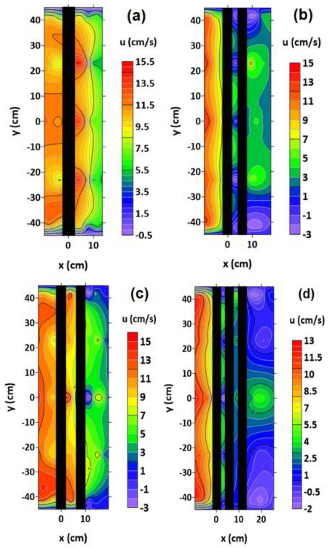
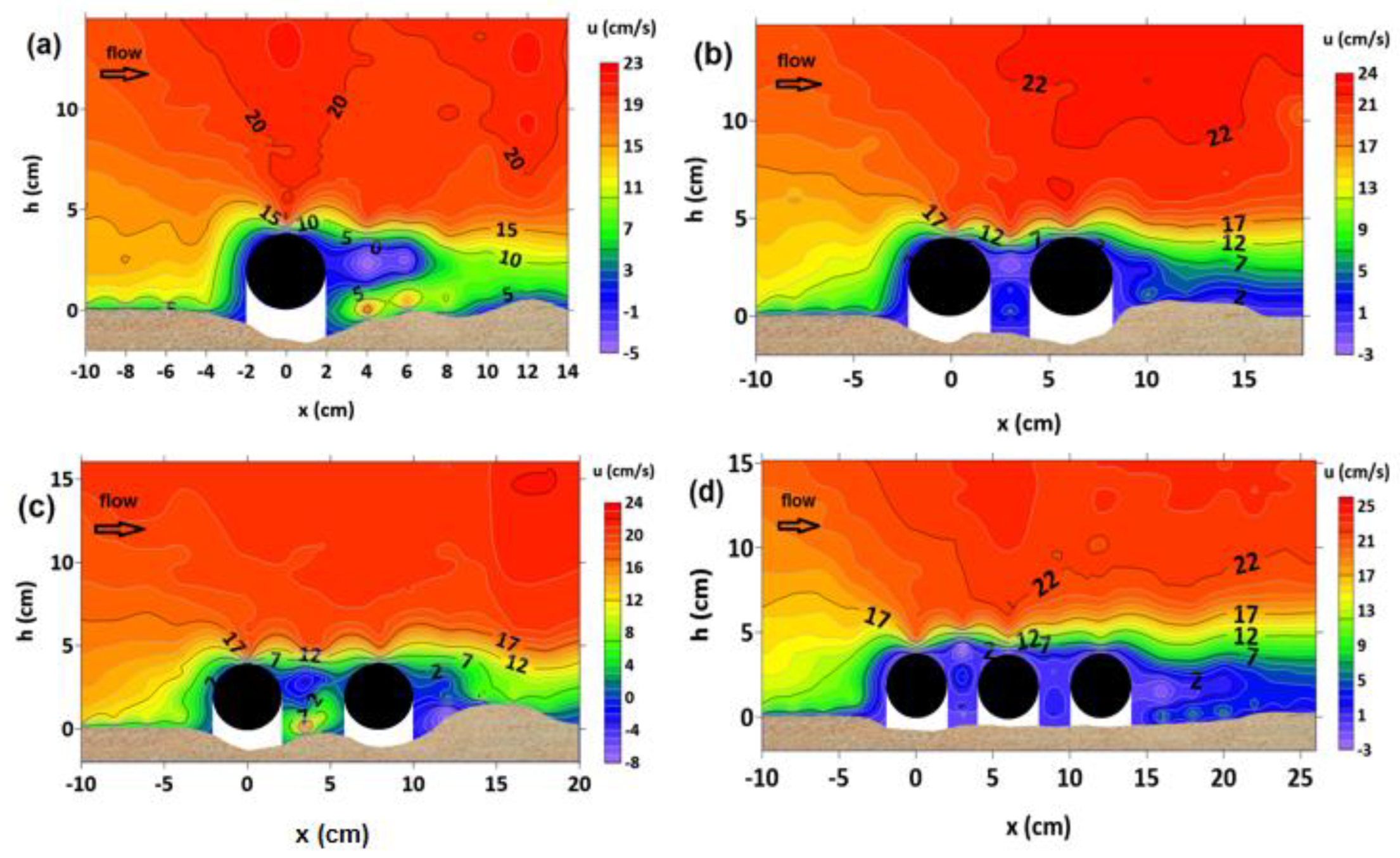
Figure 4 shows the contours of u velocity at 0.6 cm from the bed (z = 0.6 cm). Figure 4a, for the single-pipe test, shows that the horizontal component of the flow velocity (u) upstream decreases when approaching the pipe. As the flow passes through the scour hole created below the pipe, the horizontal flow velocity increases greatly, which indicates the outflow jet from under the pipe. By increasing the distance from the pipe in the area between the pipe and the sand dunes formed downstream, the horizontal velocity of the flow decreases. Additionally, after passing through the area of sand dunes, the decrease of horizontal velocity near the bed continues. For example, upstream of the pipe at the coordinates x = −10 cm, y = −23 cm, the horizontal velocity of the flow is u = 10.6666 cm/s, which near the pipe at the coordinates x = −4 cm, y = −23 cm to the value of u = 7.9887 cm/s has decreased. Downstream, the outflow jet from under the pipe, at coordinates x = 4 cm, y = −23 cm increases speed up to u = 14.1914 cm/s. Then, during a decreasing process in coordinates x = 14 cm, y = −23 cm, the value of u = 5.1011 cm/s has been reached. In this figure, reverse flow is not observed upstream and downstream of the single pipeline. By approaching the walls, the horizontal velocity values decrease, which indicates the effect of the walls. For example, in the upstream of the pipe from coordinates x = −10 cm, y = 0 to coordinates x = −10 cm, y = −42 cm, the velocity has decreased from u = 12.2335 cm/s to u = 10.1111 cm/s. Downstream of the pipe from coordinates x = 4 cm, y = 0 to coordinates x = 4 cm, y = −42 cm, the velocity decreases from u = 13.4359 cm/s to u = 9.4478 cm/s. In addition, the maximum value of the horizontal velocity at z = 0.6 cm, in this case, is u = 14.6849 cm/s, which is in the central cross-section of the channel at coordinates x = 4 cm and y = 23 cm.

In Figure 4b (state 2—two pipes with a distance of 0.5 D), the horizontal component of the velocity near the bed upstream has decreased by approaching the pipes. For example, from the coordinate x = −10 cm, y = 0 to the coordinate x = −4 cm, y = 0, it has decreased from the value of u = 13.1805 cm/s to the value of u = 8.5098 cm/s. The horizontal velocity of this flow has been significantly reduced by entering the scour hole formed in the distance between the two pipes. For example, the velocity value at coordinates x = 3 cm, y = 0 is equal to u = 0.6363 cm/s. Additionally, negative values of horizontal velocity can be seen in this area, which indicates reverse flow. For example, in the coordinates, x = 3 cm, y = −23 cm and x = 3 cm, y = −42 cm, the horizontal velocity values are u = −2.7319 cm/s and u = −2.0174 cm/s, respectively. As the flow passes through the scour hole under the second pipe to the downstream side, an increase in the velocity values is observed. Still, these values are smaller compared to the upstream flow of pipelines. For example, in the coordinates x = 10 cm, y = 0, u = 3.2508 cm/s, which show an increase compared to u = 0.6363 cm/s in the coordinates x = 3 cm, y = 0, but compared to u = 8.5098 cm/s in the upstream of the pipe at coordinates x = −4 cm, y = 0 is much less. Next, by moving away from the downstream pipe, a decreasing trend occurs in the velocity values. For example, from coordinates x = 10 cm, y = 0 to x = 18 cm, y = 0, the velocity reaches from u = 3.2508 cm/s to u = 2.3106 cm/s. According to the mentioned materials, in this tested case, due to the short distance between the two pipes, the flow has been blocked, which causes the velocity values to be small, and the reverse flow is created in this area. Comparing Figure 4a with Figure 4b shows the effect of the presence of the second pipe at a short distance from the first pipe. In other words, the second pipe’s presence has significantly reduced the horizontal velocity of the flow passing through the scour hole near the bed downstream of the pipe. The examination of the horizontal velocity values in the central axis of the channel (y = 0) show that the velocity of the outflow from under the pipe downstream in the second state at a distance of 0.5 D from the second pipe is u = 3.2508 cm/s, which compared to the first state, at the same distance from the pipe in the downstream, with the velocity u = 13.4359 cm/s, it has decreased by 75.8%. This can be a justification for less scouring depth in the second case compared to the first. The point of commonality between the two states is that the horizontal velocity values near the bed are higher in the central area of the channel, compared to the area near the walls. For example, in the upstream part, from coordinates x = −10 cm, y = 0 to coordinates x = −10 cm, y = −42 cm, the horizontal velocity value has decreased from u = 13.1805 cm/s to u = 11.0879 cm/s.

Figure 4c, which is related to the third case with two pipes with distance D, shows that the values of horizontal velocity near the bed decreased as it approached the upstream pipe. A decreasing trend is also observed downstream of the pipelines, but in the distance between two pipes, some increase in the velocity values can be seen. Downstream of the pipelines, in the area of the central axis, as well as near the walls, negative values of the horizontal velocity can be seen. For example, in the central axis of the channel (y = 0), the horizontal velocity at x = −10 cm is equal to u = 13.8888 cm/s. Then, it decreases at x = −4 cm to u = 9.1231 cm/s. At the distance between two pipes, it has values of u = 14.3719 cm/s and u = 9.1892 cm/s at x = 3.5 cm and x = 4.5 cm, respectively. Immediately downstream of the second pipe at x = 12 cm, it had a negative value of u = −4.0123 cm/s, then again from x = 16 cm to x = 20 cm, the horizontal velocity decreased from u = 8.4674 cm/s to u = 1.3925 cm/s. The maximum values of positive horizontal velocity have also been observed in the central transverse area of the channel (velocity u = 14.3719 cm/s in coordinates x = 3.5 cm, y = 0). The comparison of Figure 4a,c shows that the presence of the second pipe downstream of the first pipe has significantly reduced the horizontal velocity of the flow near the bed in the distance between the two pipes and downstream of the pipes. For example, in the central axis of the channel, at a distance of 0.5 D from the downstream pipe, u has decreased by 77.5% compared to the same distance from the downstream pipe in the first case. The same issue justifies the reduction in scouring depths in the third case compared to the single pipe case. The comparison of Figure 3b,c shows that increasing the distance between the two pipes from 0.5 D to D has caused the effect of the presence of the second pipe on reducing the horizontal flow velocity in the space between the two pipes, as well as the downstream of them, it should be weaker so that in the distance between two pipes and at the central axis of the channel, the magnitude of the horizontal velocity in the third state is 22.6 times compared to the second state. This issue is in harmony with the greater scouring depth in the third state compared to the second.

In Figure 4d (case 4: three pipes with a distance of 0.5 D) in the upstream part of the pipelines similar to previous three cases, as the flow approaches the first pipe (upstream pipe), the horizontal velocity of the flow has decreased. For example, in the central axis, it has decreased from u = 12.1336 cm/s at x = −10 cm to u = 10.6877 cm/s at x = −4 cm. When the flow enters the scour hole formed in the distance between the first and second pipe, the horizontal velocity values become negative, which indicates reverse flow. Nevertheless, in the distance between the second and third pipes, there is no effect of reverse flow, and the horizontal velocity is positive, but with a small magnitude. Downstream of the pipes, in the central axis of the channel, there has been some increase in the horizontal flow velocity (up to u = 4.4238 cm/s at x = 18 cm). In other parts, however, the horizontal velocity values are positive or negative and close to zero. By comparing this state with the second state, the values of the horizontal velocity downstream of the pipes and also in the area between the first and second pipes are almost similar to each other and a significant decrease in the horizontal velocity of the flow has been observed along with the presence of reverse flow. The difference is that the velocity values are closer to zero in the case of three pipes. Additionally, in both mentioned cases, in the central area of the channel downstream of the pipes, the velocity has increased a little. This velocity increase occurred in the case of three pipes in the central axis of the channel and other parts, there is a positive velocity close to zero or negative, but in the second case, two pipes with a distance of 0.5 D, in a larger part of the central area of the channel and the negative horizontal velocity values are limited to the parts close to the walls.

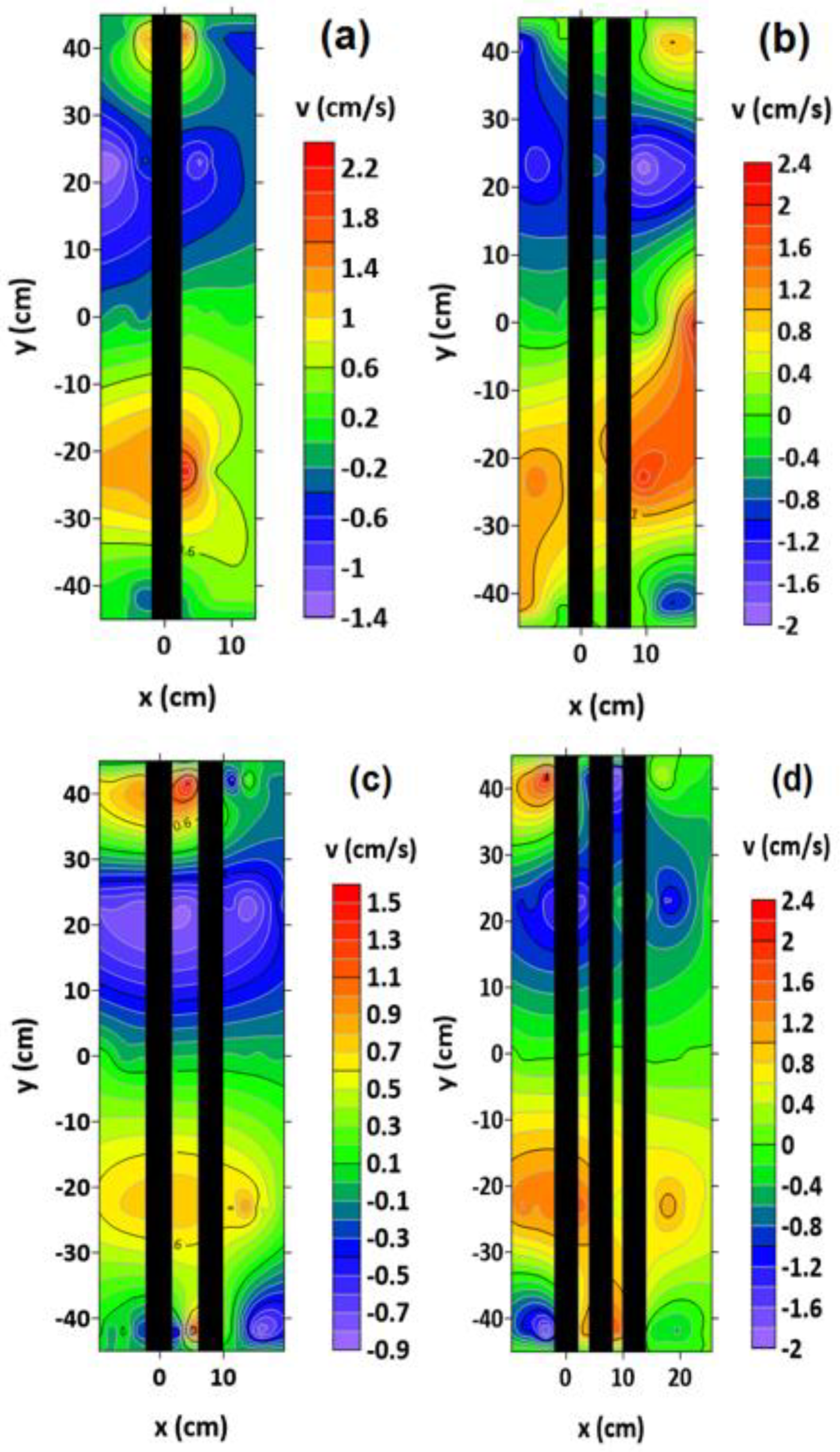
In the following, the lateral component of the velocity (v) at 0.6 cm from the bed will be investigated. In Figure 5a–d, this component is shown for the four tested cases. In all four arrangements of pipes, in the negative-y areas, v is positive (flow deviation in the counterclockwise direction) and in positive-y areas, v is negative (flow deviation in the clockwise direction). This shows the deviation of the current towards the transverse central axis of the channel (y = 0). By approaching the transverse central axis of the channel, the lateral velocity values (both positive and negative) decrease and tend to zero.

In the first test case, near the walls, at a short distance from the upstream and downstream of the pipe, some deviation of the flow towards the walls is observed. For example, at the coordinates x = −4 cm, y = −42 cm, v = −0.4678 cm/s, and at the coordinates x = 4 cm, y = −42 cm, v = −0.0118 cm/s. In the second case of the test, this deviation continues to a greater distance downstream of the pipes and the maximum value of this deviation (lateral velocity deviation towards the wall) occurred at a distance of 1.5 D from the pipe to the downstream side (value v = −1.0465 cm/s in coordinates x = 14 cm, y = −42 cm and the value of v = 1.0555 cm/s in coordinates x = 14 cm, y = 42 cm). In the third case of the test, the deviation of the flow towards the wall is observed in the upstream parts, the distance between the two pipes, and the downstream. The maximum value of deviation in the distance of 1.5 D downstream of the second pipe at the coordinates x = 16 cm, y = −42 cm is equal to v = −0.8228 cm/s, and between the pipes at the coordinates x = 4.5 cm, y = 42 cm to the value of v = 1.6554 cm/s. In the fourth case of the test, the deviation of the lateral component of the flow velocity towards the wall was created only in the upstream and downstream of the pipelines. (The maximum value of deviation at x = −4 cm, y = −42 cm is equal to v = −2.0067 cm/s and at x = −4 cm, y = 42 cm is equal to v = 2.3256 cm/s).

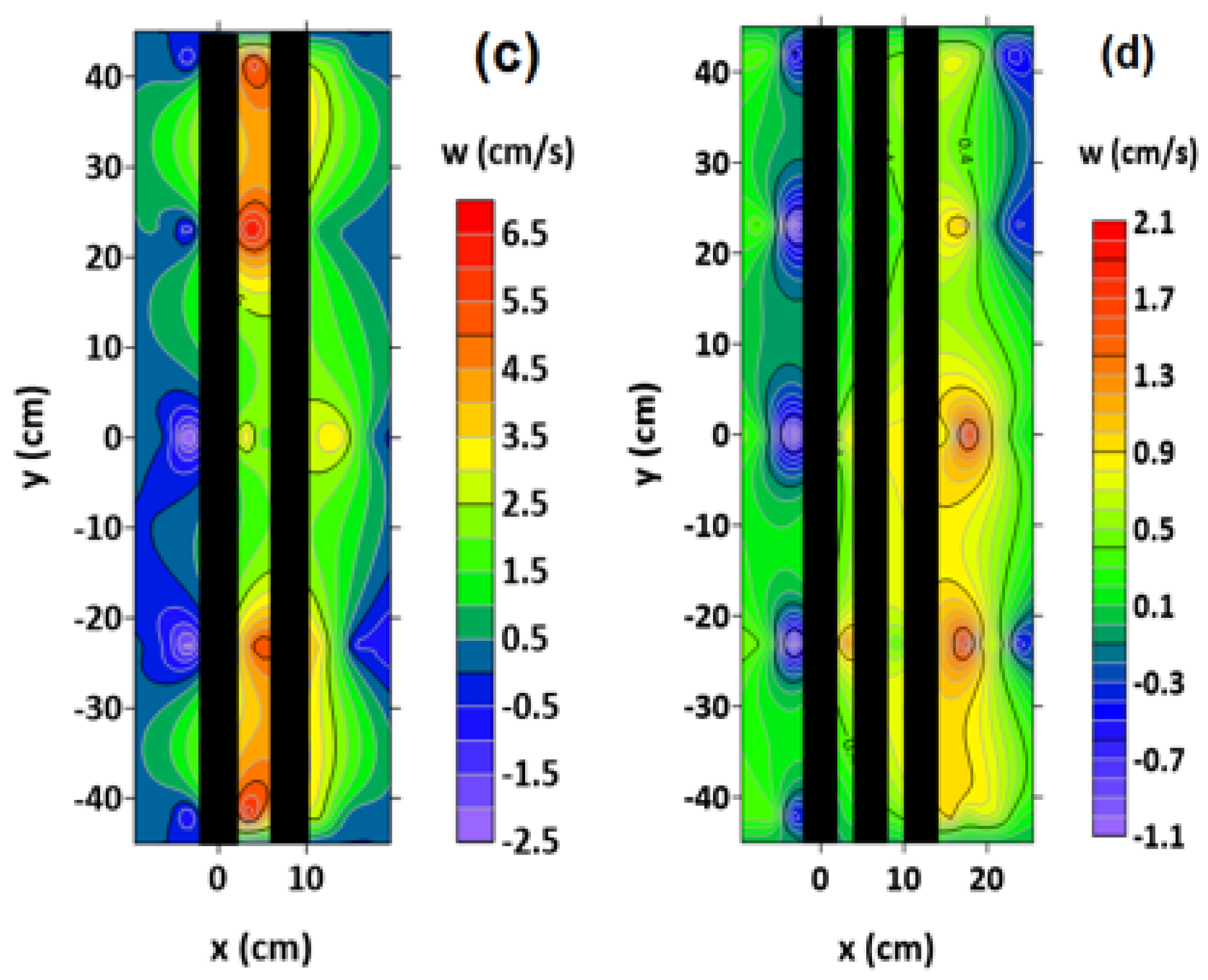
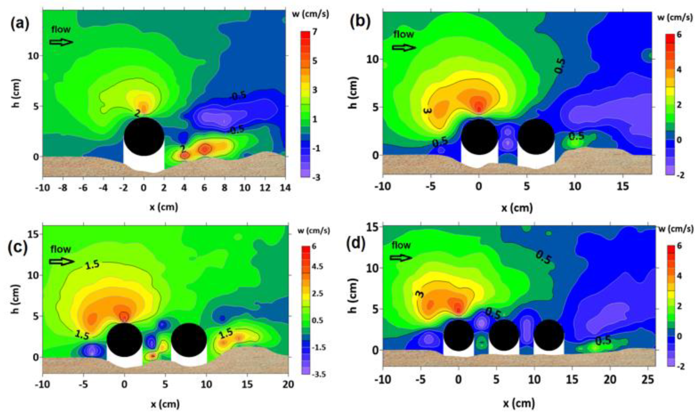
In Figure 6a–d, the contours are presented for the vertical component of the velocity at 0.6 cm from the bed. Results show that an upward flow is formed upstream of the pipes, which can be caused by the separation of the flow. By approaching the pipeline, negative values of the vertical velocity are observed, which can be due to the flow entering the scour hole. Downstream of the pipelines, an upward flow has occurred due to the exit from the scour hole. In the following, this flow faces the sand dunes formed downstream of the pipe(s), and the values of the vertical component of the velocity remain positive. Gradually, passing through the positive slope of the sand dunes and approaching their peak, the values of the vertical velocity tend to zero, and then, upon reaching the negative slope of the sand dunes, the values of the vertical component of the velocity become negative.

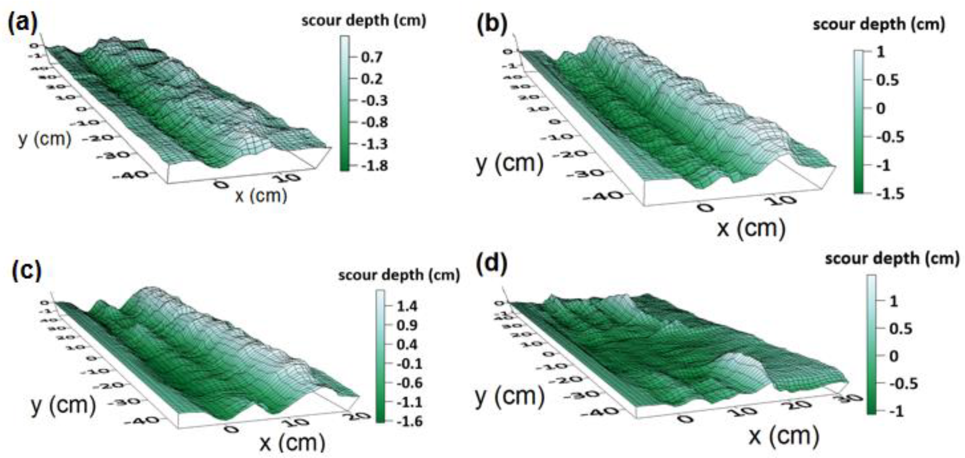
The highest values of the vertical component of the velocity downstream of the pipe are observed in the first state (single pipe) (the maximum value of w = 9.8877 cm/s in coordinates x = 4 cm, y = −23 cm). This problem can be justified considering that the depth of the scour hole in the first case is greater than the other three cases, and the flow downstream of the single pipe must exit from a deeper hole. The maximum positive values of the vertical component of the velocity among the other three states, as expected, are related to the third state (two pipes with section D), which has the highest scour depth after the first state. These large positive values of vertical velocity, in addition to the downstream of the pipelines (the maximum value of w = 3.6357 cm/s at the coordinates x = 14 cm, y = 0 at the distance D from the downstream pipe), are also observed in the area between the two pipes. (The maximum value of w = 6.8709 cm/s in coordinates x = 3.5 cm, y = −42 cm). This can be caused by the outflow of the flow from the scour hole created under the first pipe. Additionally, the vortices created in the distance between two pipes can be the cause of these vertical velocity values. In the second case of the test, the maximum positive values of the vertical component of the flow velocity formed downstream of the pipes are lower than the first and third cases (the maximum value of w = 2.4222 cm/s in coordinates x = 10 cm and y = −23 cm in the distance 0.5 D from the downstream pipe). Between the two pipes, unlike the third case, the velocity in the vertical direction has positive values but with a small magnitude. In the fourth case, the maximum positive values of the vertical component of the velocity created downstream of the pipes are lower than in the second case (the maximum value of w = 1.9882 cm/s in coordinates x = 18 cm, y = −23 cm at the distance D from the downstream pipe). This issue indicates the gentle slope of the scour hole in this area. In the distance between the pipes in the fourth state, like the second state, the vertical velocity has positive values but with a small magnitude. The mentioned discussion and results are in agreement with the results obtained from the scour hole in all cases.

3.3.2. Velocity Field in X-Z Plane

Figure 7a shows that upstream of the pipe (x = −10 cm to x/D = −2.5), the effect of the presence of the pipe on the flow path is less, the horizontal component of the flow velocity near the bed becomes larger as z increases, and by moving away from the bed, the horizontal velocity gradient decreases. When approaching the pipe, the effect of the pipe on blocking the flow is quite evident. The gradient of the horizontal component of velocity u is intense on the pipe and the value of the velocity has increased from the number close to zero to the velocity u = 20.7743 cm/s at 0.5 cm from the upper surface of the pipe. Furthermore, with the increase of z, not much change occurs in the horizontal velocity values. The shear layer of the flow passing over the pipe, by separating from its surface downstream, has formed two vortices during the interaction with the shear layer exiting from under the pipe. Additionally, in Figure 7a, the negative values of the horizontal velocity in this area indicate the existence of reverse flow. According to Zhang et al. (2016) [9], the formation of reverse flow indicates the presence of the two mentioned vortices in the flow area of the pipeline wake. Gradually, with the distance from the pipe downstream, the effect of the pipe’s presence on the flow is reduced, and the horizontal velocity changes at different depths, becoming like the flow at a large distance upstream of the pipe. Downstream of the pipe and near the bed, the u values increase. Abbaszadeh Tavassoli and Haji Kandi. (2010) [6] point out the increase in velocity in this area and considered it to be the cause of the scour hole downstream of the pipeline. Yeganeh Bakhtiari et al. (2011) [7] also state that vortex shedding occurs downstream. Brors (1999) [21] has investigated the velocity contours around the single pipe after the scour cavity has reached equilibrium which are very similar to the contour lines of Figure 7a.

In Figure 7b, contours for the horizontal component of the velocity in the second stage of the test are shown. In this case, like the first case, the horizontal component of the velocity has decreased by approaching the pipelines. In the areas on the pipes, a strong horizontal velocity gradient is also observed, and this gradient is higher on the first pipe than on the second pipe. At 0.5 cm from the upper surface of the first pipe, u = 20.4537 cm/s, and at the same distance from the upper surface of the second pipe, u = 15.6927 cm/s. With a sharp increase in velocity in these areas, there is no significant velocity gradient further when increasing z. Downstream of the pipes, the reverse flow was not observed, but in the distance between the pipes, with increasing distance from the bed, the positive values of the horizontal velocity are initially small. At the distances of 3.3 and 3.8 cm from the bed, the reverse flow is observed with the values of u = −1.7599 cm/s and u = −1.9538 cm/s. In the following, the values of the horizontal velocity are again positive but with a small magnitude. In this area, approaching the height level of the upper surface of the pipes (h = 4 cm), a strong gradient has occurred in the velocity values, so that the velocity u = 3.7643 cm/s at z = 4.4 cm is reached u = 19.0666 cm/s at z = 5 cm. After reaching the maximum velocity, there is no significant change in the velocity values. Hu et al. (2019) [22], during an experiment on the scouring of two parallel pipes in a shallow flow, pointed out the formation of the maximum velocity at a short distance from the upper surface of the pipes.

In Figure 7c, third test case, by approaching pipelines from the upstream side, the horizontal velocity values decrease. Additionally, a strong gradient of u is observed in the area on the pipes. In this case, like the second case, the velocity gradient on the upper surface of the first pipe is stronger than the second pipe, so that, up to a distance of 0.5 cm from the upper surface of the first pipe, the horizontal velocity is u = 19.1342 cm/s and up to the same distance from the upper surface in the second pipe, the velocity has reached u = 15.6726 cm/s. After this sharp increase in velocity in these areas, the u changes are small as z increases. Downstream of the pipelines, in the areas near the bed up to z = 2.2 cm, there was a reverse flow with the maximum value of u = −7.8705 cm/s at x = 12 cm, z = 0.3 cm. Then, with the increase of z, there is no effect of the reverse flow, and the horizontal component of the velocity is faced with a high gradient in the positive direction. Additionally, in the area between the second pipe and the sand dune, a reverse flow is formed, but with the increase of x, there is no effect of the reverse flow in the areas on the dune. Moving downstream, negative values of horizontal velocity near the bed are also observed downstream of the sand dune (with a maximum value of u = −0.1539 cm/s at x = 20 cm, z = 0.3 cm). In the area between the two pipelines, a sharp increase in the positive u values near the bed has occurred. A little above this area, in the range of z = 2 cm to z = 4 cm, negative u values have been created. This issue shows the interactions caused by the collision of shear layers separated from the upper and lower surfaces of the first pipeline. This process, like the process occurring downstream of the single pipe (case 1), has caused the creation of two vortices in this area. By comparing the third and second states, it seems that the increase in the distance between the two pipes has caused the shear layer to separate from the upper and lower surfaces of the first pipe to have enough space to mix in between the two pipes and form two vortices. Near the bed, there has been enough space to create a strong horizontal velocity gradient by the outflow jet from under the first pipe. These vortices can be considered as the Carman vortices that Ishigai et al. (1972) [23] mentioned in their study.

Figure 7d shows the u contours for the fourth tested case. In the upstream of the pipelines, like the previous cases, the horizontal component of velocity u has decreased as it approaches the upstream pipe. On the upper surface of the pipes, a strong horizontal velocity gradient is observed, which decreases on the second and third pipes, respectively. After this extreme gradient, with the increase of z, no noticeable change in u values is observed. In the distance between the first and second pipe, like the second case, u values are small and do not fluctuate significantly. At z = 0.9, 4.3, 4.8 cm, the reverse flow was created with the values of u = −1.8244, −2.9317, −2.9228 cm/s, respectively, and in the rest of the elevated levels of this area, the velocity was positive, but its magnitude was small. The reason for this can be seen in the previous cases, because of the flow’s stagnation due to the small distance between the pipes. This flow stagnation is much greater in the distance between the second and third pipes. In this area, there is no sign of reverse flow and the horizontal velocity values are all positive, and at the same time, very close to zero. In the downstream of the pipelines, the values of the horizontal component of the velocity are positive with a small magnitude, and only in the cross section of x = 16 and in the height range of 1.5 cm ≤ z ≤ 2.3 cm, the presence of reverse flow is observed (−2.0353 cm/s ≤ u ≤ −0.6308 cm/s). Near the bed, the horizontal velocity values also increase slightly.

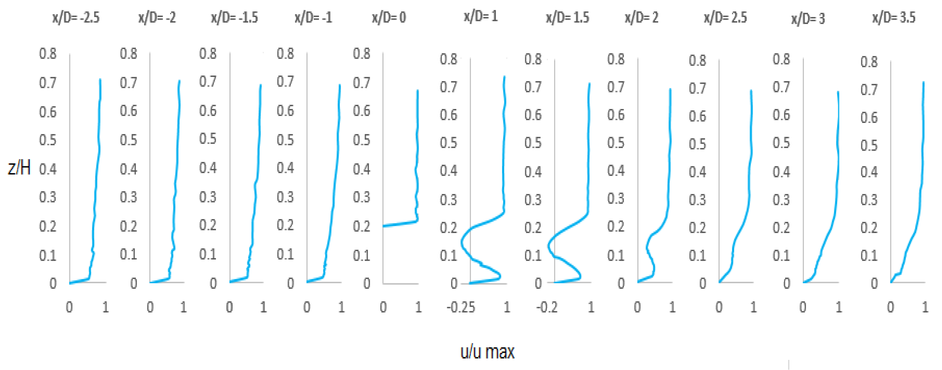
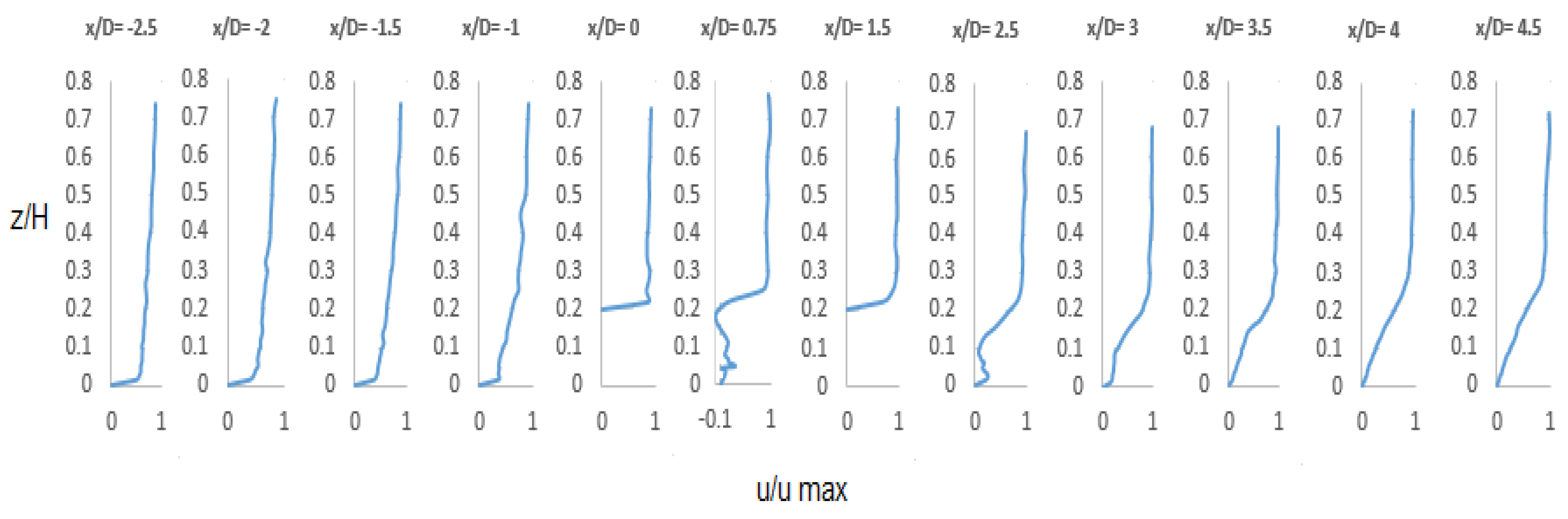
Figure 8 shows the dimensionless profiles of the horizontal component of the velocity in the direction of the flow u, in the upstream, downstream, and on the single pipe, after the bed balance. Examining the velocity profiles in sections x/D = −1.5, −2, and −2.5 shows that the effect of the pipe’s presence on the horizontal velocity profile far upstream is insignificant. At section x/D = 0, a high velocity gradient can be seen on the pipe. In this area, the velocity at a distance close to the pipe almost reaches the maximum value ($\mathrm{u} =0.97 {\mathrm{u}}_{\max }$), and further, with the increase of z, no significant changes in the velocity values are observed. In sections x/D = 1.5 and x/D = 1, S-shaped profiles are formed, which indicate two vortices in this area of the flow due to the presence of negative horizontal velocity values in them. In section x/D = 2, the S-shaped profile is still observed, but there is no reverse flow. In the next sections (x/D = 2.5, 3, 3.5), gradually, there is no more S-shaped profile, and the effect of the pipe’s presence on the velocity profiles becomes less and less. A similar general trend in the changes of the velocity profiles formed around the single pipe can be seen in the studies of researchers such as Jensen et al. (1990) [2], Zhang et al. (2016) [9], and Chen et al. (2020) [10], so the results of the single pipe case are similar to previous studies in this field.

By comparing the velocity profile at x/D = 3.5 and x/D = −2.5, the velocity gradient near the bed at x/D = 3.5 is much lower compared to x/D = −2.5. At x/D = 3.5, the velocity has approached the maximum value at a greater distance from the bed (at z/H = 0.26, u value has reached $\mathrm{u}=0.82 {\mathrm{u}}_{\max }$). The reason for this can be the continuation of the effect of the shear layer separated from the upper surface of the pipe to a significant distance downstream of the pipe, which Figure 7a also illustrates. Moving downstream, the thickness of the boundary layer will be similar to its thickness at a long distance upstream of the pipe, and the effect of the pipe’s presence on the flow will disappear to a great extent. This matter is seen in the study of Chen et al. (2022) [13]. Zhang and Shi (2016) [8] have observed the S-shaped horizontal velocity profile and the occurrence of two vortices, during the investigation of the flow around a single pipe with an initial distance of 0.1 D, 0.3 D and 0.5 D from the bed, at the sections of x/D = 1 and x/D = 3.5 (downstream of the pipe).

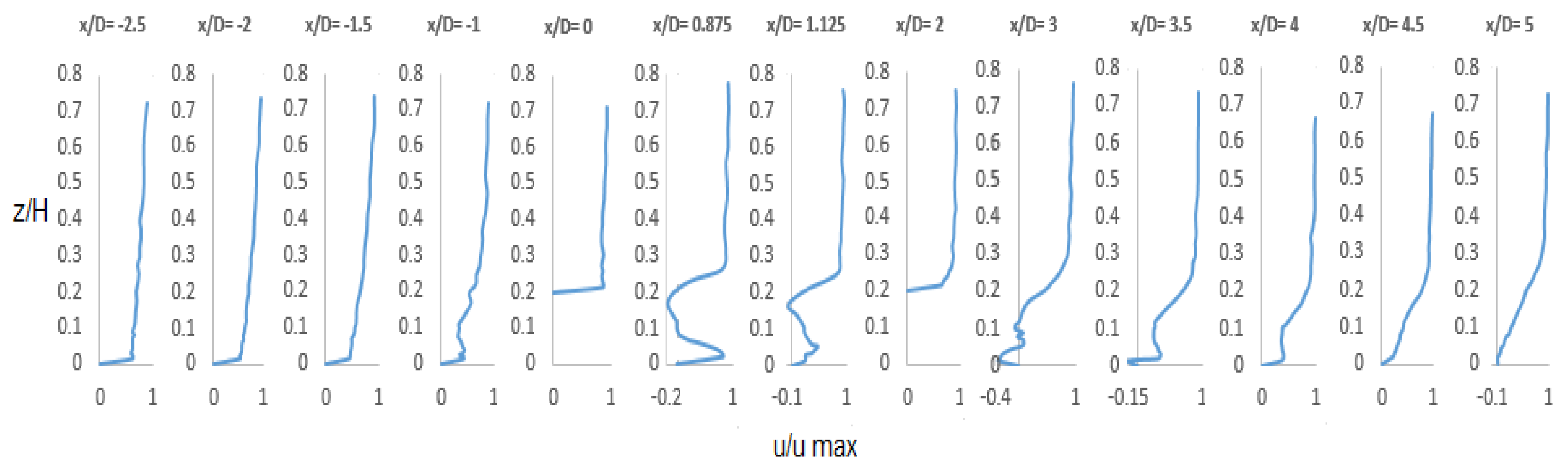
Figure 9 and Figure 10 show the dimensionless profiles of the horizontal component of the velocity around the pipelines for the study’s second and third cases. Examining these profiles in sections of x/D = −2.5, −2 and −1.5 shows that the effect of the presence of pipelines on the horizontal component of velocity in this range is negligible in both tested cases. In section x/D = −1, due to the presence of the pipe in the flow path, a decrease in the horizontal velocity values is observed in the range of z/H ≤ 0.2. By comparing the velocity profiles of this section in Figure 9 and Figure 10, near the bed, the velocity values are higher in Figure 10 (state 3). For example, in z/H = 0.015 in the third state, $\mathrm{u} =0.4275{ \mathrm{u}}_{\max }$ and at the same z/H in the second case, the horizontal velocity is $\mathrm{u} =0.3606 {\mathrm{u}}_{\max }$, which can be due to the absence of the flow stagnation between the pipes in the third case. As a result, the flow passes more freely through the scour cavity formed below the upstream pipe. The profiles of sections x/D = 0, 1.5 in Figure 9 and sections x/D = 0 and 2 in Figure 10 show the extreme velocity gradient on the pipes. The profile of section x/D = 0.75 in Figure 9 (between two pipes) shows irregularities in the values of u near the bed. In this area, these values are positive and have a small magnitude. With the increase in z, first, the horizontal velocity moved towards negative values, reaching $\mathrm{u}=-0.08 {\mathrm{u}}_{\max }$, and then in the range close to the level of the upper surface of the pipelines, a sharp increase was found in the positive direction so that, at z/H = 0.25, the value of $\mathrm{u}=0.83 {\mathrm{u}}_{\max }$. After that, with the increase of z, there was no significant change in u values. At the same time, in sections x/D = 0.875 and 1.125 in Figure 10, S-shaped profiles were formed, which have negative velocity values and indicate the presence of Carman vortices. In the section x/D = 2.5, in Figure 9, which is the area immediately downstream of the downstream pipe (corresponding to the second state of the test), an S-shaped profile is observed, but there is no negative value in the velocity values. While in section x/D = 3 in Figure 10, which shows the area immediately downstream of the pipelines (related to the second test case), the S-shaped profile is not formed, and at the same time, near the bed, the velocity values are negative. In the height range of the presence of the pipe ($\mathrm{z}/\mathrm{H}\le 0.2$), irregularity is observed in the horizontal velocity profile. In the next sections and moving downstream (Figure 9 and Figure 10), the influence of the pipelines on the horizontal velocity profiles gradually decreases. Of course, as mentioned in the description of the velocity profiles related to the first case (single pipe), until a relatively large distance downstream of the pipe(s), the velocity profiles are still unlike the upstream of the pipes, and the thickness of the shear layer is greater. This thickness gradually decreases, until the velocity profiles become like the velocity profiles upstream away from the pipelines.

Figure 11 shows the dimensionless profiles of the horizontal velocity, corresponding to the fourth case. In this case, in the section x/D = −1, in the height range of the presence of the pipe, a decrease in the horizontal velocity values is observed. The comparison of the velocity profiles in the sections at x/D = 0, x/D = 1.5, and x/D = 3 shows that the intensity of the vertical gradient of the horizontal velocity $\left(\frac{\mathrm{du}}{\mathrm{dz}}\right)$ on the upper surfaces of the first to third pipes (respectively) decreases relatively. In the cross section x/D = 0.75, which corresponds to the area between the first and second pipes, as z increases from near the surface of the bed, there have been fluctuations in the horizontal velocity values that do not follow a specific order. At the same time, except for the two areas where the graph entered negative values, in the rest of the range between the two pipes (z < 4), the graph is very close to the vertical axis and only fluctuates in positive values and close to zero. This can be attributed to the stagnation effect of the flow in this area due to the small distance of the pipes. This effect is more observable in the cross section of x/D = 2.25 (between the second and third pipes), so that in part z < 4, the graph is close to the vertical axis and the horizontal velocity values have very small fluctuations. The maximum value of the horizontal velocity in this part is equal to $\mathrm{u}=0.084{ \mathrm{u}}_{\max }$ at z/H = 0.045. The reason for this can be considered the presence of the third pipe at 0.5 D from the second pipe, which has aggravated the flow stagnation in the area between the pipes. Downstream of the pipes, S-shaped profiles are also observed, but only in the section of x/D = 4 reverse flow with the maximum value of $\mathrm{u}=-0.084{ \mathrm{u}}_{\max }$ is created at z/H = 0.105. By moving downstream, the S-shaped profiles gradually disappear in the next sections, and no trace of the S-shaped profile can be observed in sections x/D = 6 and 6.5.

Figure 12 shows the contours of the transverse component of velocity (v) for four test conditions. As expected, due to the symmetry of the elements in the transverse direction of the channel in the experiments of this study (horizontal pipelines), the flow examination in the x-z plane in the transverse central axis of the channel shows that the values of v are very small and there is only a slight flow deviation to the left or right. In Figure 12a, which is related to the first case (single pipe), an almost two-dimensional flow is formed upstream of the pipeline. Of course, in the area behind the pipe, the transverse deviation of the flow increases slightly. Downstream, the v values increase slightly, which can be attributed to the outflow jet from under the pipe, the presence of Carman vortices in the pipe wake, and the presence of sand dunes. In Figure 12b (the second case), in the gap between the two pipes, some deviation of the flow in the transverse direction is observed. Additionally, in the downstream areas of the sand dunes and near the pipe and the bed upstream of the first pipe, an increase in the lateral deviation of the flow is observed. In the rest of the parts, the values of the transverse component of the velocity are very low or zero. In Figure 12c, the third case, the transverse velocity tends to zero in most parts. More deviation in the transverse flow is observed in parts such as the upstream flow near the bed (behind the first pipe), the distance between two pipes (with the presence of Carman vortices), and downstream of the pipelines. In Figure 12d, the fourth case, in the downstream parts of the pipelines, upstream points near the first pipe, and the space between the pipes, the lateral deviation of the flow is slightly increased.

Figure 13 shows the contours of the vertical component of the velocity (w) for four test conditions. In the upstream part and close to the pipe, the separation of the flow into two parts is clearly defined. The first part is the downward flow near the bed (w < 0), which can indicate the flow entering the scour cavity, and the second part is the upward flow (w > 0) that passes over the upper surface of the pipe. Downstream, the flow passing over the upper surface of the pipe is first horizontal and then downwards. The upward flow of the outlet from under the pipe is also observed near the bed. The values of the vertical component of the velocity in the distances between the pipes (in the second to fourth states) near the bed have become positive, and with a slight distance from it (increasing z), the vertical velocity has become negative. In the second and fourth case, these values are small. In the third case, when the two pipes are placed at a greater distance from each other, the shear layers separate from the upper and lower surfaces of the first pipe have more room to move in the space between the two pipes. In this case, an upward jet flow is observed near the bed, and immediately above it, a downward flow is observed, which has led to the formation of Carman vortices in this area. The maximum downward velocity in this part is w = −2.1905 cm/s in coordinates x = 3.5 cm, z = 1.9 cm, and the maximum upward velocity in this part is w = 4.5353 cm/s in coordinates x = 3.5 cm, z = 0.6 cm.

4. Discussion

In this study, scouring under the pipelines in four arrangements (cases) was investigated: (1) single pipe, (2) two pipes with a distance of 0.5 D, (3) two pipes with a distance of D, (4) three pipes with a distance of 0.5 D, in a direct channel with a uniform flow and H/D = 5 (H is the depth of flow). Additionally, horizontal, vertical, and lateral components of flow velocity were measured using ADV around the four arrangements. The results show:

1-

The magnitude of the horizontal component of the velocity near the bed for four tested cases matches with the results of their maximum scour depth.

2-

In the first case, downstream of the pipeline, the existence of S-shaped profiles along with the negative values of horizontal velocity in sections x/D = 1 and x/D = 1.5 show that vortices are formed in this area.

3-

In the second case, the reverse flow was not observed downstream of the pipelines, but in the distance between the two pipes, at distances of 3.3 and 3.8 cm from the bed. In general, in the area between the two pipes, the magnitude of the velocity is close to zero, which is caused by the small distance between the pipes and, as a result, the flow stagnated to a large extent in this area.

4-

In the third case, in the distance between two pipes, large positive horizontal velocity values were observed near the bed, and reverse flow in the range of z = 2 cm to z = 4 cm. S-shaped horizontal velocity profiles can also be seen in this area, which are formed due to the presence of two vortices. This process is similar to the process that happens downstream of the single pipe and is caused by the sufficient distance between the pipes for the interaction of the shear layers. Downstream of the pipelines, in this case, near the bed, the reverse flow was observed up to z = 2.2 cm, and after that, positive horizontal velocity was observed. S-shaped profiles are not formed in this area.

5-

In the fourth case, in a distance between the pipes, the effect of flow stagnation is observed. Downstream of the pipelines, there are S-shaped profiles of horizontal velocity, but negative horizontal velocity was observed only in the section of x/D = 4, 1.5 cm ≤ z ≤ 2.3 cm.

5. Conclusions

This study represents an advancement in the current understanding of the flow-structure interaction at scoured horizontal pipelines (especially in two-pipe and three-pipe arrangements) subjected to currents. It was demonstrated that the maximum and minimum scour depth among the four pipe arrangements examined in this study is formed in single-pipe and three-pipe arrangements, respectively. As a result, the use of pipe groups at a distance of 0.5 D has effectively reduced the maximum scour depth. This study indicates that the scouring depth under the pipelines is in harmony with the velocity components in the horizontal and vertical directions (u and w), and changing the arrangement of pipelines significantly changes the rate of these velocity components. Additionally, by comparing the arrangements of two pipes with a distance of 0.5 D and three pipes with a distance of 0.5 D, it seems that increasing the number of pipes will lead to lower scouring. Considering that in most practical projects, the pipe groups are used under the sea, where the bed material is fine sand. The results of this study will therefore be helpful for designers.

Over the last few decades, various methods have been proposed and investigated to protect pipelines from scouring. Some designers prefer to bury the pipelines under the seabed in order to protect them. One of the advantages of this method is to protect the pipeline against lateral movements caused by currents and sea waves. However, with the burial of the pipeline, the possibility of physical inspection of the pipeline is eliminated and some problems are created in its maintenance stages. A number of researchers have used other protection methods, such as using horizontal or vertical impermeable plates, to control erosion under pipelines, particularly for the one and two pipeline cases. The results of their studies show that the use of these plates is effective in reducing scouring.

In this study, the focus is on the best arrangement of pipelines that are directly placed on the erodible bed with sand materials with a size of ${\mathrm{d}}_{50}=0.83$ mm. Additionally, the results show that the way the pipelines are placed on the bed is very important. However, in cases where the bed materials are finer and more exposed to scouring, it is recommended to use the best arrangement of pipelines along with an efficient protection method, which is expected to bring better results.

References

1. Bearman, P.W.; Zdravkovich, M.M. Flow around a circular cylinder near a plane boundary. J. Fluid Mech. 1978, 89, 33–47. [Google Scholar] [CrossRef]
2. Jensen, B.L.; Sumer, B.M.; Jensen, H.R.; Fredsoe, J. Flow around and forces on a pipeline near a scoured bed in steady current. J. Offshore Mech. Arct. Eng. 1990, 112, 206–213. [Google Scholar] [CrossRef]
3. Lei, C.; Cheng, L.; Kavanagh, K. Numerical Flow Visualization of Vortex Shedding Flow Over a Circular Cylinder Near a Plane Boundary. In Proceedings of the Ninth (1999) Interna onal Offshore and Polar Engineering Conference, Brest, France, 30 May–4 June 1999. [Google Scholar]
4. Oner, A.A.; Kirkgoz, M.S.; Akoz, M.S. Interaction of a current with a circular cylinder near a rigid bed. Ocean. Eng. 2008, 35, 1492–1504. [Google Scholar] [CrossRef]
5. Lin, W.J.; Lin, C.; Hsieh, S.C.; Dey, S. Flow characteristics around a circular cylinder placed horizontally above a plane boundary. J. Eng. Mech. 2009, 135, 697–716. [Google Scholar] [CrossRef]
6. Abbaszadeh Tavassoli, A.; Haji Kandi, H. Investigating the flow after creating scour holes under oil pipelines using Fluent software. In Proceedings of the 9th Hydraulic Conference of Iran, Tarbiat Modares University, Tehran, Iran, 8 November 2010. [Google Scholar]
7. Yeganeh Bakhtiari, A.; Kazemi Nejad, M.; Hosseini Ghahi, H. Investigation of scouring and hydrodynamic forces on transmission pipelines under the effect of flow. In Proceedings of the National Conference of New Finding in Civil Engineering, Nagaf Abad, Iran, 23 February 2010. [Google Scholar]
8. Zhang, Z.; Shi, B. Numerical simulation of local scour around underwater pipelines based on fluent software. J. Appl. Fluid Mech. 2016, 9, 711–718. [Google Scholar] [CrossRef]
9. Zhang, Z.; Shi, B.; Guo, Y.; Chen, D. Improving the prediction of scour around submarine pipelines. Marit. Eng. 2016, 169, 163–173. [Google Scholar] [CrossRef] [Green Version]
10. Chen, L.; Wang, Y.; Sun, S.; Wang, S. The effect of boundary shear flow on hydrodynamic forces of a pipeline over a fully scoured seabed. Ocean Eng. 2020, 206, 107326. [Google Scholar] [CrossRef]
11. Penna, N.; Coscarella, F.; Gaudio, R. Turbulent flow field around horizontal cylinders with scour hole. Water 2020, 12, 143. [Google Scholar] [CrossRef] [Green Version]
12. Liu, M.M.; Jin, X.; Wang, L.; Yang, F.; Tang, J. Numerical investigation of local scour around a vibrating pipelines under steady currents. Ocean Eng. 2021, 221, 108546. [Google Scholar] [CrossRef]
13. Chen, W.; Ji, C.; Alam, M.M.; Xu, D.; Zhang, Z. Three-dimensional flow past a circular cylinder in proximity to a stationary wall. Ocean Eng. 2022, 247, 110783. [Google Scholar] [CrossRef]
14. Goring, D.G.; Nikora, V.I. Despiking acoustic Doppler velocimeter data. J. Hydraul. Eng. 2002, 128, 117–126. [Google Scholar] [CrossRef] [Green Version]
15. Wahl, T. Analyzing ADV data using WinADV. In Proceedings of the Joint Conference on Water Resources Engineering and Water Resources Planning and Management, Minneapolis, MN, USA, 30 July–2 August 2000; pp. 1–10. [Google Scholar]
16. Mao, Y. The Interaction between a Pipeline and an Erodible Bed; Series Paper Technical University of Denmark; Technical University of Denmark: Lyngby, Denmark, 1986. [Google Scholar]
17. Li, Y.; Ong, M.C.; Fuhrman, D.R.; Larsen, B.E. Numerical investigation of wave-plus-current induced scour beneath two submarine pipelines in tandem. Coast. Eng. 2020, 156, 103619. [Google Scholar] [CrossRef]
18. Westerhorstmann, J.H.; Machemehl, J.L.; Jo, C.H. Effect of pipe spacing on marine pipeline scour. Presented at the Second International Offshore and Polar Engineering Conference, San Francisco, CA, USA, 14 June 1992; Volume II, pp. 101–109. [Google Scholar]
19. Gao, F.P.; Yang, B.; Wu, Y.X.; Yan, S.M. Steady current induced seabed scour around a vibrating pipeline. Appl. Ocean Res. 2006, 28, 291–298. [Google Scholar] [CrossRef] [Green Version]
20. Maddah, S.; Kolahdouzan, F.; Eftekhari, A.; Singh, V.P.; Afzalimehr, H. Experimental Investigation of Scouring in Groups of Parallel Pipelines. Int. J. Hydraul. Eng. 2021, 10, 27–34. [Google Scholar]
21. Brors, B. Numerical modeling of flow and scour at pipelines. J. Hydraul. 1999, 125, 511–523. [Google Scholar] [CrossRef]
22. Hu, D.; Tang, W.; Sun, L.; Li, F.; Ji, X.; Duan, Z. Numerical simulation of local scour around two pipelines in tandem using CFD–DEM method. Appl. Ocean Res. 2019, 93, 101968. [Google Scholar] [CrossRef]
23. Ishigai, S.; Nishikawa, E.; Nishimura, K.; Cho, K. Experimental Study of Structure of Gas Flow in Tube Bank Swith Tube Axes Normal to Flow (Part I, Karman Vortex Flow from Two Tubes at Various Spacings); Bulletin of the JSME 15; The Japan Society of Mechanical Engineers: Tokyo, Japan, 1972; pp. 949–956. [Google Scholar]
Figure 1. The location of the single pipe and measuring points in the longitudinal direction of the flume.
Water 15 01321 g001
Figure 2. Topography of the final scouring hole around the pipelines: (a) single pipe, (b) two pipes G/D = 0.5, (c) two pipes G/D = 1, (d) three pipes G/D = 0.5.
Water 15 01321 g002
Figure 3. Centerline longitudinal bed profile at equilibrium: (a) single pipe, (b) two pipes G/D = 0.5, (c) two pipes G/D = 1, (d) three pipes G/D = 0.5.
Water 15 01321 g003
Figure 4. Velocity field around the pipelines in the X-Y plane at height of 0.6 cm from the scour bed (u, cm/s): (a) single pipe, (b) two pipes G/D = 0.5, (c) two pipes G/D = 1, (d) three pipes G/D = 0.5. Note that the range of the color scale is not equalized for better illustration.
Water 15 01321 g004
Figure 5. Velocity field around the pipelines in the X-Y plane at height of 0.6 cm from the scour bed (v, cm/s): (a) single pipe, (b) two pipes G/D = 0.5, (c) two pipes G/D = 1, (d) three pipes G/D = 0.5. Note that the range of the color scale is not equalized for better illustration.
Water 15 01321 g005
Figure 6. Velocity field around the pipelines in the X-Y plane at height of 0.6 cm from the scour bed (w, cm/s): (a) single pipe, (b) two pipes G/D = 0.5, (c) two pipes G/D = 1, (d) three pipes G/D = 0.5. Note that the range of the color scale is not equalized for better illustration.
Water 15 01321 g006aWater 15 01321 g006b
Figure 7. Velocity field around the pipelines in the X-Z plane (u, cm/s): (a) single pipe, (b) two pipes G/D = 0.5, (c) two pipes G/D = 1, (d) three pipes G/D = 0.5. Note that the range of the color scale is not equalized for better illustration.
Water 15 01321 g007
Figure 8. Profiles of normalized velocity u in different sections for the case of single pipe.
Water 15 01321 g008
Figure 9. Profiles of normalized velocity u in different sections for the case of two pipes G/D = 0.5.
Water 15 01321 g009
Figure 10. Profiles of normalized velocity u in different sections for the case of two pipes G/D = 1.
Water 15 01321 g010
Figure 11. Profiles of normalized velocity u in different sections for the case of three pipes G/D = 0.5.
Water 15 01321 g011
Figure 12. Velocity field around the pipelines in the X-Z plane (v, cm/s): (a) single pipe, (b) two pipes G/D = 0.5, (c) two pipes G/D = 1, (d) three pipes G/D = 0.5. Note that the range of the color scale is not equalized for better illustration.
Water 15 01321 g012
Figure 13. Velocity field around the pipelines in the X-Z plane (w, cm/s): (a) single pipe, (b) two pipes G/D = 0.5, (c) two pipes G/D = 1, (d) three pipes G/D = 0.5. Note that the range of the color scale is not equalized for better illustration.
Water 15 01321 g013