Estimation of the Peak over Threshold-Based Design Rainfall and Its Spatial Variability in the Upper Vistula River Basin, Poland

Abstract

The proper assessment of design rainfalls with long return periods is very important because they are inputs for many flood studies. In this paper, estimations are performed on daily design rainfall totals from 16 meteorological stations located in the area of the Upper Vistula River Basin (UVB), Poland. The study material consists of a historical series of daily rainfall totals from the period of 1960–2021. The peak over threshold (POT) method is used, and the rainfall depth over threshold is assumed to follow the generalized Pareto distribution (GPD) with parameters estimated from Hill statistics. Alternatively, the competitive method based on annual maxima (AM) is applied. The theoretical distribution of AM is assumed to follow a theoretical distribution function selected by using the Akaike information criterion (AIC) from a family of seven candidate distributions, the parameters of which are estimated by using the maximum likelihood method. The two methods are compared by using the root mean square error (RMSE) and the mean deviation error (MDE) criteria. It is found that the POT-based method with GPD and Hill estimators outperform the AM-based method when considering the highest rainfall events. The confidence intervals of the design rainfalls, derived by using the Monte Carlo simulation method, reflects their large spatial diversity across the UVB. It is shown that the station’s altitude strongly correlates with the threshold, variance, and design rainfall depth of the GPD. This proves the advantage of the GPD with Hill estimates, namely that it can accurately reflect the spatial properties of rainfall and its variability in the UVB. Results can be applied in water-management applications related to floods.

1. Introduction

Intense and long-duration precipitation has caused many catastrophic flood events in Poland, such as those seen in 1970, 1997, 2001 and 2010. In addition, as [1] indicates, the number of local flash floods resulting from heavy rainfalls has increased in Poland. The increasing urbanization process and climate changes have caused long periods of drought and then heavy rainfall, which may cause a further increase in the frequency and intensity of floods in the future. Currently, more and more emphasis is placed not only on the drainage of rainwater, but on its retention, as well as reproduction of retention lost as a result of the catchment sealing process [2]. Because of this, accurate designing of high rainfall depths is a pressing issue.

The proper modeling of extreme precipitation in the Upper Vistula River Basin (UVB), located in the southern part of Poland, is of high importance because the region is very flood prone. In the region, the estimation of design rainfall totals for long return periods is crucial for designing storm water drainage or land drainage systems, and preparing flood risk maps, as well as planning flood-control solutions [3]. The rationale for this study is that rivers in most of the region are very susceptible to flooding, the contribution of the surface runoff from this area to the total surface runoff of Poland is very high, and that, due to climate change, rainfall has become more and more intense in recent years.

Much attention should be given to the proper estimation of the distribution of daily rainfall totals because the right tail of the probability density function (PDF) is highly influenced by the observed high-precipitation quantiles. From the point of view of hydrology and meteorology, it is crucial to learn whether the tail of the PDF is heavy or light [4,5]. A heavy tail of the distribution indicates that the probability of occurrence of very high precipitation is larger than for a light tail.

The main objective of the paper was to conduct a very precise estimation of daily design rainfall depth for various return periods. The approach was not based on the commonly used annual maxima (AM) method but on the peak over threshold (POT) method with the use of Hill statistics. In the POT-based method, all sample values that exceed a certain threshold level are accounted for. The daily precipitation depth over this threshold was assumed to follow the generalized Pareto distribution (GPD). The Hill estimators of the parameters were used in the GPD fit. The estimators can accurately reflect very high rainfall values, often observed in the UVB. We also addressed the issue of the spatial associations between orography and variance of the GPD, and design rainfall depths. To assess the quality of the POT-based estimation with Hill statistics, we also performed the AM-based estimation by using the maximum likelihood and compared the results. Different distribution functions, such as the generalized extreme value (GEV), two-parameter gamma (Pearson 3, GA2), three-parameter gamma (GA3), lognormal (LOG), two-parameter Weibull (WE2), three-parameter Weibull (WE3), and Gumbel (GUM) were considered in the AM-based method in this study.

In Poland, the Bogdanowicz–Stachý probabilistic maximum precipitation model for various return periods is often used [6,7,8]. This AM-based method makes use of the Weibull distribution, the parameters of which reflect some specific rainfall properties in three different regions of Poland. However, the model does not cover the southern, mountainous part of the UVB with very high precipitation totals. Moreover, recent climatic changes might also affect its suitability [9].

The POT approach enables an increase of the sample size in comparison to the AM-based method by considering all independent peak events over threshold and the omission of low values below threshold which are not valid in the estimation of large events. This is the main advantage of the POT approach in comparison with the AM approach. The disadvantages are the inclusion of subjective judgment into the POT sample selection and the GPD estimation, and the strong sensitivity of high quantile estimates to the threshold choice. Therefore, the main difficulties in selecting the POT sample are the choice of the threshold, which produces the lowest bias of quantile estimates, and the ensured independence between successive events [10,11].

The GPD was used in various fields of study [12,13]. For instance, Madsen et al. [14,15,16] demonstrated that the POT-based GPD fit leads to a more accurate estimation of high quantiles compared to the AM-based GEV fit. Van Montfort and Witter [17] indicated that in the GPD fit, some POT series of daily rainfall show exponentially distributed peaks, with one or more outlying observations [17]. The methodology of developing the Polish Atlas of Rains Intensities (PANDa) (see [2]) was also based on the GDP distribution; however, the method of parameter estimation substantially differs from the method based on the Hill statistics in this paper. Various methods have been used in meteorology and hydrology to calibrate the GPD. For example, Madsen and Rosbjerg [18] compared the method of moments, probability-weighted moments, and maximum likelihood (ML) with regard to the precision of the 100-year flood quantile estimate. Martins et al. [19] used the ML estimates for the assessment of extreme monthly rainfall in Brazil. Singirankabo [20] applied the ML method to daily rainfall intensity in Rwanda. Martins and Stedinger [21] used the generalized maximum likelihood (GML) method, in which the ML and Bayesian approaches are combined, in extreme flood assessment. Yet another method of the GPD parameters’ estimation was adapted by Willems et al. to river discharges [22]. They used the Hill estimator of the $\gamma$ parameter [23,24]. The Hill estimates were then successfully applied to river discharges and rainfall intensities in various world regions [11,25,26,27,28]. The main advantages of the method are that (i) the calibration of the threshold is based directly on sample values, which is crucial because of the large spatial diversity of rainfalls in the UVB, and (ii) the parameter estimation is weighted toward large rainfall events that play an important role in designing extremely heavy rainfalls. This method was used in the paper.

2. Materials and Methods

2.1. Study Area and Data

The Upper Vistula River Basin (UVB) has a total surface area of 47,053.51 km${}^2$ (the Polish part; see Figure 1). It is diverse in terms of altitudes and geological structure (it includes the Carpathians, a part of the Carpathian Foredeep, parts of the Lublin Basin, the Upper Silesia Basin, the Cracow Monocline, the Nida Basin, and a part of the Świętokrzyskie Mountains). The spatial distribution of precipitation varies from the lowest in the north to the highest in the south (the Tatra Mountains). The meteorological conditions are influenced by polar maritime air masses in the west and continental air masses in the east; thus the climate is transitional [29,30,31]. The strong diversity in climate conditions influences the volume of precipitation and its extreme values. As indicated by Młyński et al. [32], the occurrence of precipitation is characterized by seasonality. In the UVB, the highest rainfall most often occurs in summer (from May to September). The region is very susceptible to flooding [33,34]. Additionally, as the UVB makes up approximately 30% of water resources in Poland [35], the region plays an important role in flood generation in a large part of the country [31].

The region is heavily influenced by anthropogenic activity [36]. It includes, e.g., a part of the Silesian urban area, which constitutes an important industrial region, as well as large cities: Kraków, Rzeszów, Tarnów, and many hydrotechnical structures (e.g. Wisła Czarne, Goczałkowice, Czorsztyn-Niedzica, Solina).

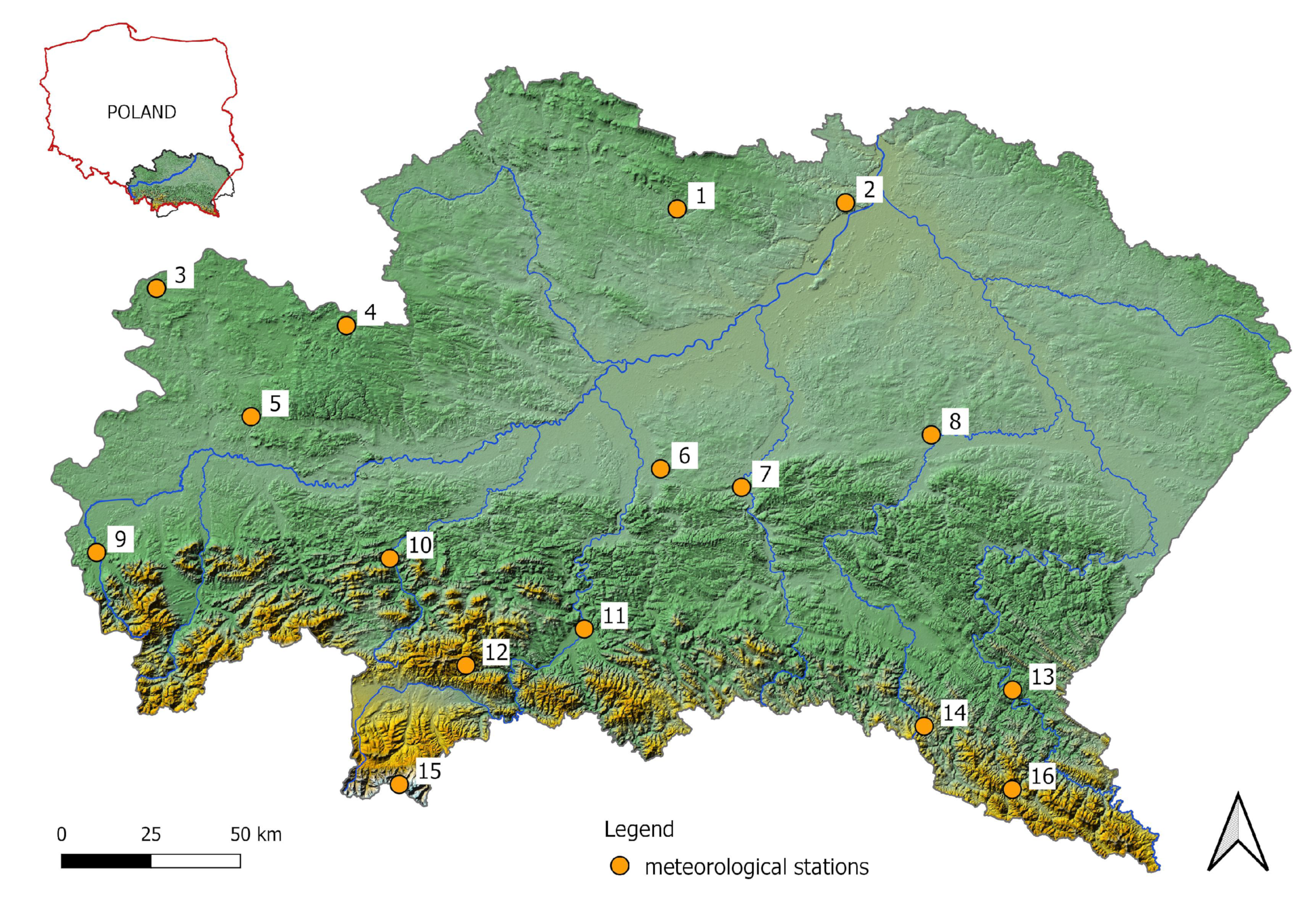
In the study, the stations located at the lowest altitudes are Rzeszów-Jasionka (200 m. a.s.l), Tarnów (209 m. a.s.l) and Pilzno (210 m. a.s.l), whereas Ochotnica Górna (620 m. a.s.l) and Kasprowy Wierch (1991 m. a.s.l, the Tatra Mountains) are at the highest altitudes (

Table 1. The stations used in the study and their main characteristics [37,38].

No.	Station	Longitude	Latitude	Altitude [m. a.s.l.]	Mean dp ${}^{\left(1\right)}$ [mm]	Mean AM ${}^{\left(2\right)}$ [mm]
1	Raków	21${}^{\circ }$03′00″	50${}^{\circ }$41′00″	220	1.63	36.14
2	Sandomierz	21${}^{\circ }$42′57″	50${}^{\circ }$41′48″	217	1.55	38.44
3	Brynica	19${}^{\circ }$00′00″	50${}^{\circ }$28′00″	285	2.03	41.53
4	Wolbrom	19${}^{\circ }$45′00″	50${}^{\circ }$23′00″	370	2.06	43.03
5	Chrzanów	19${}^{\circ }$23′00″	50${}^{\circ }$09′00″	295	2.10	42.60
6	Tarnów	20${}^{\circ }$59′04″	50${}^{\circ }$01′48″	209	1.97	49.71
7	Pilzno	21${}^{\circ }$18′00″	49${}^{\circ }$59′00″	210	1.98	46.64
8	Rzeszów-Jasionka	22${}^{\circ }$02′32″	50${}^{\circ }$06′39″	200	1.76	37.79
9	Skoczów	18${}^{\circ }$47′42″	49${}^{\circ }$47′56″	295	2.59	53.84
10	Stróża	19${}^{\circ }$56′00″	49${}^{\circ }$48′00″	307	2.54	51.37
11	Nowy Sącz	20${}^{\circ }$41′21″	49${}^{\circ }$37′38″	292	2.01	45.14
12	Ochotnica Górna	20${}^{\circ }$14′00″	49${}^{\circ }$32′00″	620	2.32	50.48
13	Lesko	22${}^{\circ }$20′30″	49${}^{\circ }$27′59″	420	2.24	42.96
14	Wisłok Wielki	21${}^{\circ }$59′57″	49${}^{\circ }$22′44″	550	2.64	49.95
15	Kasprowy Wierch	19${}^{\circ }$58′55″	49${}^{\circ }$13′57″	1991	4.89	83.01
16	Cisna	22${}^{\circ }$20′00″	49${}^{\circ }$13′00″	540	2.98	52.47

⁽¹⁾ Daily precipitation ⁽²⁾ Annual maximum.

).

The series of daily precipitation totals from the period between 1960 and 2021 from 16 meteorological stations located in the UVB were used for the analysis (Figure 1). The data were obtained from the public database of the Institute of Meteorology and Water Management, National Research Institute (IMGW-PIB). In days with snowfall, the rainfall equivalent is provided in the data. Therefore, rainfall and precipitation are equivalent in the paper.

The mean value of the annual maximum daily rainfall total in the period between 1960 and 2021 varied from 36.14 mm (Raków) to 83.01 mm (Kasprowy Wierch) while the mean daily precipitation ranged from 1.5 mm to 2.10 mm, apart from Kasprowy Wierch, for which it was 4.89 mm (see Table 1).

2.2. Research Methods

The POT-based method with Hill statistics was applied in the design rainfall estimation. Then, for comparative purposes, the AM-based method was also used. The superior method was selected next in the sense that a higher rating was given to the method that better estimated the highest rainfall depths. Afterward, the dependence between the distribution parameters and orographic characteristics of the region where the rainfall stations are located was found.

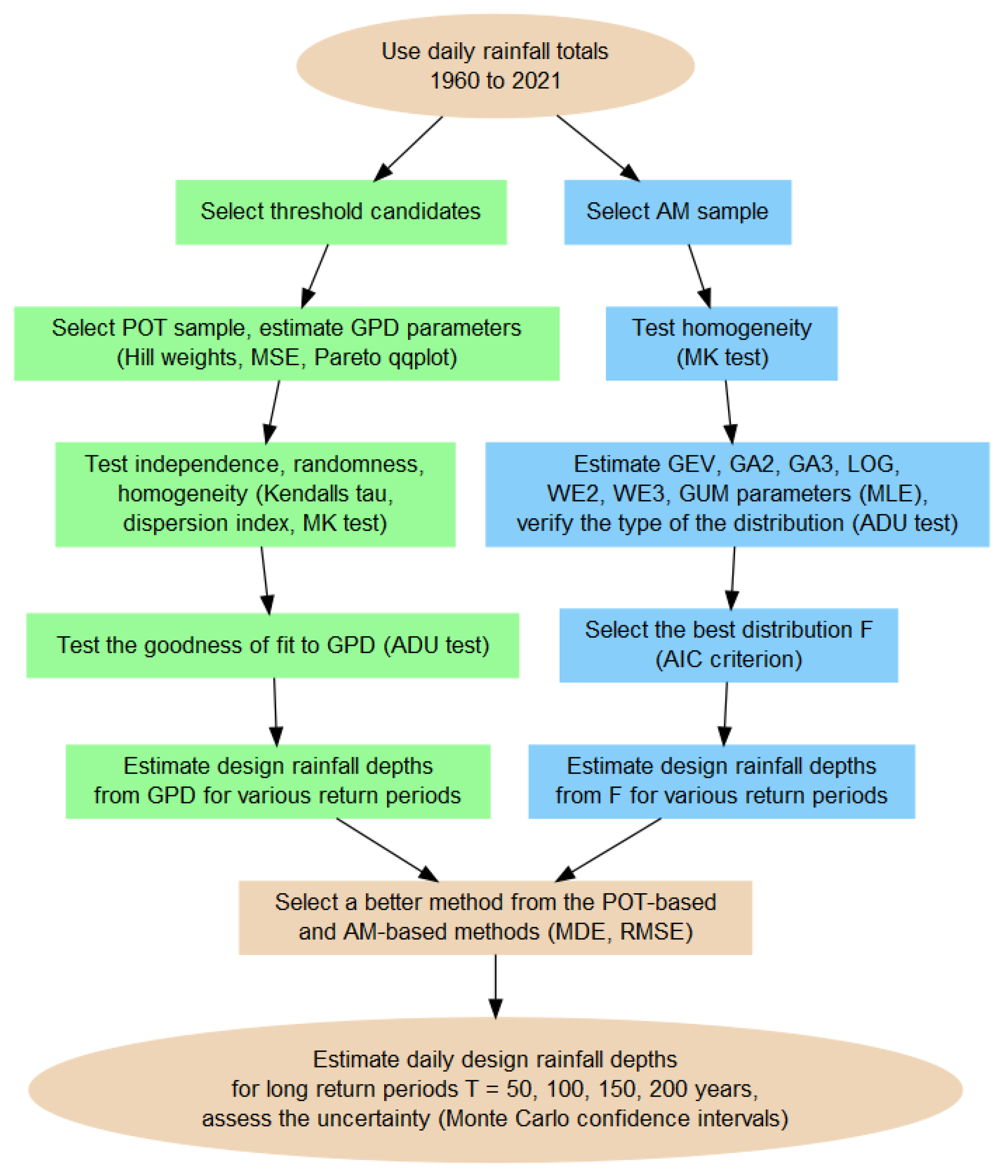
The methods were depicted in the flow diagram in Figure 2. The shapes on the left branch refer to the steps in the POT-based estimation while the shapes on the right branch refer to the AM-based estimation. The branches join when the methods are compared, the design rainfalls and their confidence intervals are estimated, and when the GPD properties are associated with orographic characteristics. The detailed description of the methods is provided in the next sections.

2.3. The POT-Based Estimation

In the POT-based method, the daily rainfall depth X over a certain threshold $x_t$ (where $X>x_t$) is assumed to follow the generalized Pareto distribution (GPD). The GPD can cover a wide range of tail weights, and therefore it is very useful in the extreme value analysis [10]. The cumulative distribution function (CDF) of the GPD equals

$$G\left(x\right)=\left\{\begin{array}{cc}1-{(1+\gamma \frac{x-x_t}{\sigma })}^{-\frac{1}{\gamma }}\hfill & \mathrm{if}\gamma \ne 0,\hfill \\ 1-\exp (-\frac{x-x_t}{\sigma })\hfill & \mathrm{if}\gamma =0\hfill \end{array},\right.$$

(1)

where $\gamma \in R$ is the shape parameter and $\sigma >0$ is the scale parameter. The $\gamma$ parameter is known as the extreme value index. The scale parameter linearly depends on the threshold $x_t$, with proportionality factor equal to the shape parameter, namely $\sigma =\gamma x_t$, if only $x_t$ is sufficiently high [24]. A high, positive value of the $\gamma$ parameter (heavy tail of the distribution) indicates that the probability of the occurrence of very high precipitation is larger than if $\gamma =0$ (light, exponential tail). The variance of GPD equals

$$Va{r}_{\mathrm{GPD}}=\frac{{\sigma }^2}{{(1-\gamma )}^2(1-2\gamma )}(\mathrm{if}\gamma <\frac{1}{2}).$$

(2)

As the values of the estimated maximum precipitation depth and their variability strongly depend on $\sigma$ and $\gamma$, its precise estimation is therefore highly important, especially in the areas susceptible to heavy downpours and torrential storms.

The POT-based estimation consisted of several steps the methods of which are provided the the following subsections.

2.3.1. Selection of the POT Sample

In order to select the final POT sample, various threshold candidates had to be considered. Before this, all daily precipitation totals greater than or equal to the lowest annual maximum AM (initial value) in the period between 1960 and 2021 were selected. Subsequently, to address the issue of the serial correlation of daily rainfall totals, the Kendall’s $\tau$ coefficient was tested for significance [39] for lag = one day. At the stations where the correlation was significantly different from zero (Sandomierz, Stróża, Kasprowy Wierch), the series were then modified by taking only the days with at least one day of temporal distance. Strictly speaking, if two rainfall depths from two consecutive days were included in the first sample, the lower value was omitted. This modification enabled the selection of the series with uncorrelated elements. No modification was carried out for stations with uncorrelated rainfall events. Then, for each station, the series was ordered from the lowest to the highest, $x_t⩽∆⩽x_1$ with the lowest AM as the initial threshold value. This was the series of all threshold candidates.

Afterward, starting from the lowest element $x_t$, the threshold was successively increased and, in each step, the Hill estimate $\widehat{\gamma }$ of the shape parameter $\gamma$ of the GPD distribution was estimated [40]:

$$\widehat{\gamma }=\frac{1}{t-1}\sum _{j=1}^{t-1}ln{x}_j-ln{x}_t.$$

(3)

The estimate $\widehat{\gamma }$ is the mean excess of the log-transformed data over the threshold $x_t$. The asymptotic mean squared error was also computed in each step [40],

$$MSE=\frac{1}{t-1}\sum _{j=1}^{t-1}{w}_j{(ln\frac{x_j}{x_t}-\widehat{\gamma }ln\frac{t}{j})}^2,$$

(4)

assuming the Hill weights $w_j=-\frac{1}{ln\frac{j}{t}},j=1,2,\dots ,t-1$. The threshold $x_t$ for which the series of the $MSE$ achieved minimum was the final, optimal threshold. The final choice of the threshold was a tradeoff between low thresholds, which cause a high bias, and high thresholds, which cause a high variance of $\widehat{\gamma }$; therefore the selection of $x_t$ from the region of low fluctuation of $\widehat{\gamma }$ was of high importance. The final POT sample comprised of the POT events greater than or equal to the final threshold $x_t$. The appropriate choice of $x_t$ was verified in the Pareto QQ plot where the points $(-ln\left(p_j\right),ln\left(x_j\right))$ for $p_j=\frac{j}{t+1}$—the probability of exceedance of $x_j$—should lay along the regression line with the slope equal to $\widehat{\gamma }$ if the true distribution of the rainfall depth above threshold is GPD. This is the main advantage of the Hill weights, namely that the regression line is pulled toward matching the largest rainfall events because the Hill estimation is pointed at the events with a low probability of exceedance.

If the fit in the Pareto QQ plot is poor, because the points for the highest rainfall events lie much below the regression line, this means that the tail of the empirical distribution should be fitted to the GPD with $\gamma =0$ (exponential distribution, EXP) where the estimate of the scale parameter equals [40]

$$\widehat{\sigma }=\frac{1}{t-1}\sum _{j=1}^{t-1}{x}_j-x_t.$$

(5)

In this case, the optimal threshold $x_t$ was selected based on minimizing the $MSE$ [40]:

$$MSE=\frac{1}{t-1}\sum _{j=1}^{t-1}{w}_j{(x_j-x_t-\widehat{\sigma }ln\frac{t}{j})}^2.$$

(6)

The exponential QQ plot is $(-ln\left(p_j\right),x_j)$, where $p_j=\frac{j}{t+1}$, was also used to assess the goodness of fit. The method was described in [40,41] and applied in [11,22,26].

The final estimates of the location, scale, and shape parameters of the GPD were $x_t,\widehat{\sigma },\widehat{\gamma }$, where $\widehat{\gamma }$ was derived from the Equation (3) and $\widehat{\sigma }=\widehat{\gamma }{x}_t$, while the estimates of the location and scale parameters of the exponential distribution were $x_t,\widehat{\sigma }$ where $\widehat{\sigma }$ was derived from the Equation (5).

2.3.2. Testing the Independence, Randomness, and Homogeneity

Many procedures for the POT series selection often suffer from some subjectivity; therefore, an objective criterion of independence, randomness, and identical distribution of the POT events should be included.

For various lags, the hypothesis that the Kendall’s $\tau$ serial correlation of the POT sample is zero [39] was verified. In order to check the randomness of the POT events, the method based on the dispersion index $\Psi =\frac{{\sum }_{i=1}^{n_y}{(y_i-\overline{y})}^2}{\overline{y}}$ was used to verify the hypothesis that the distribution of the number of exceedances over threshold per year is Poisson [10,42,43]. From a theoretical point of view, $\Psi$ should asymptotically follow a ${\chi }^2$ distribution with $n_y-1$ degrees of freedom where $y_i,\overline{y},n_y$ is the number of exceedances over threshold, its mean value, and the number of years, respectively.

Afterward, all final POT series were tested for homogeneity in the parameter of location by using the Mann–Kendall (MK) test for trend [44,45].

2.3.3. Testing the Goodness of Fit to the GPD Distribution

In order to verify the hypothesis that the distribution of rainfall depth over threshold was GPD, the Anderson–Darling (AD) test [46] was used in its modified version which accounts for the upper tail of the probability distribution function, namely [47],

$$\mathrm{ADU}=\frac{t}{2}-2\sum _{j=1}^{t}G\left(x_{\left(j\right)}\right)-\sum _{j=1}^t(2-\frac{2j-1}{t})ln(1-G\left(x_{\left(j\right)}\right)),$$

(7)

where G is the cumulative distribution function of the GPD (see the Equation (1)). The critical values ADU${}_{\mathrm{crit}}$ of the AD test were estimated by using the Monte Carlo method based on $N={10}^4$ simulations.

2.3.4. Estimating the Design Rainfall Depth

Assuming that $\mu$ is the mean number of the POT elements per year, the return period of the rainfall depth x is $T\left(x\right)=\frac{1}{\mu (1-G(x\left)\right)}$. By using this equation, the design rainfall of return period T was derived from

$$x_{GPD}\left(T\right)=\left\{\begin{array}{cc}{x}_t{\left(T\mu \right)}^{\gamma }\hfill & \mathrm{if}\gamma >0,\hfill \\ x_t+\sigma ln\left(\mu T\right)\hfill & \mathrm{if}\gamma =0,\hfill \end{array}\right.$$

(8)

assuming that $\mu T>1$.

2.4. The AM-Based Estimation

The steps were similar to those from the Section 2.3. The difference was in the method of estimation that made use of Hill statistics in the POT-based method and the maximum likelihood estimation in the AM-based method.

2.4.1. Testing the Homogeneity of AM

The AM series was tested for trends by using the MK test. This is an important issue in order to check whether due to climate change or other circumstances the distribution of the daily annual maxima totals did not change during the observation period.

2.4.2. Parameter Estimation and Verification of the Type of the Distribution

The family of theoretical distribution function candidates, $\mathcal{F}=\{$GEV, GA2, GA3, LOG, WE2, WE3, GUM} was considered at each station where the abbreviations apply to generalized extreme value, two-parameter gamma, three-parameter gamma, lognormal, two-parameter Weibull, three-parameter Weibull, and Gumbel, respectively. The parameters were estimated by using the MLE [48,49]. The equations for the distribution functions are commonly used in the literature [50,51,52].

For every $F\in \mathcal{F}$, the null hypothesis was verified at each station by using the Anderson–Darling test (ADU test), for which the following distribution function is F.

2.4.3. Selection of the Best Distribution of the AM and Estimation of Design Rainfall Depths

For each station, the best distribution F was selected from all distributions for which the null hypothesis was not rejected. The final selection was based on the Akaike information criterion [53,54], namely on the minimization of $AIC=-2lnL+2k$ where L is the likelihood function and k is the number of parameters of the theoretical distribution function. The main advantage of the use of $AIC$ is that it meets the principle of parameter parsimony because it combines both the L-based fit and the number of parameters. Thus, models with many parameters are penalized and have less of a chance to be selected.

After the best distribution, F was selected, and design rainfall depths for various return periods were estimated.

2.5. Selection of a Better Method from the POT-Based and AM-Based Methods

The comparison was performed between the results of two methods of estimation of the highest design rainfalls—the POT-based method and the AM-based method, the former using the Hill estimation of the GPD distribution from the POT sample (Section 2.3) and the latter using the MLE of the F distribution that was selected by using the AIC criterion (Section 2.4). The evaluation of each method was done by using the mean deviation error ($MDE$) and the root mean squared error ($RMSE$), where the observed and theoretical rainfall depths of the same return period of the GPD and F distributions were compared. We have

$$MD{E}_{POT}=\frac{1}{\#S}\sum _{T\in S}\left(x_{POT}\left(T\right)-x_{GPD}\left(T\right)\right),MD{E}_{AM}=\frac{1}{\#S}\sum _{T\in S}\left(x_{AM}\left(T\right)-x_F\left(T\right)\right)$$

(9)

$$RMS{E}_{POT}=\frac{1}{\#S}\sum _{T\in S}^{}{(x_{POT}\left(T\right)-x_{GPD}\left(T\right))}^2,RMS{E}_{AM}=\frac{1}{\#S}\sum _{T\in S}^{}{(x_{AM}\left(T\right)-x_F\left(T\right))}^2,$$

(10)

where $x_{POT}\left(T\right),x_{AM}\left(T\right)$ are the observed quantiles of return period T in the POT and AM series, respectively, while $x_{GPD}\left(T\right),x_F\left(T\right)$ are the estimated quantiles of the return period T of the GPD and F distribution, respectively. The set S consists of various return periods and $\#S$ is the number of its elements. Only long return periods were included in S to account for the highest rainfalls, namely $S_1=\{2,5,10,12,15,20,30,60\}$ years (case 1) and $S_2=\{15,20,30,60\}$ years (case 2).

The choice of the $MDE$ and $RMSE$ was due to the fact that they reflect the bias and the variance of the quantile estimators. For example, if $MD{E}_{POT}$ and $RMS{E}_{POT}$ are near to zero, it means that the bias and variance of the estimator $x_{GPD}$ is low, and the design rainfall depths are estimated properly.

The POT-based and AM-based methods were assessed in the sense that the scores $d_{1,i},d_{2,i}$ were assigned first to each station i, namely

$$d_{1,i}=\left\{\begin{array}{cc}1\mathrm{for}\mathrm{POT}\mathrm{and}0\mathrm{for}\mathrm{AM}\hfill & \mathrm{if}|MD{E}_{POT}|<|MD{E}_{AM}|\hfill \\ 0\mathrm{for}\mathrm{POT}\mathrm{and}1\mathrm{for}\mathrm{AM}\hfill & \mathrm{if}|MD{E}_{POT}|>|MD{E}_{AM}|\hfill \\ 0\mathrm{for}\mathrm{POT}\mathrm{and}0\mathrm{for}\mathrm{AM}\hfill & \mathrm{if}|MD{E}_{POT}|=|MA{E}_{AM}|\hfill \end{array},\right.$$

(11)

$$d_{2,i}=\left\{\begin{array}{cc}1\mathrm{for}\mathrm{POT}\mathrm{and}0\mathrm{for}\mathrm{AM}\hfill & \mathrm{if}RMS{E}_{POT}<RMS{E}_{AM}\hfill \\ 0\mathrm{for}\mathrm{POT}\mathrm{and}1\mathrm{for}\mathrm{AM}\hfill & \mathrm{if}RMS{E}_{POT}>RMS{E}_{AM}\hfill \\ 0\mathrm{for}\mathrm{POT}\mathrm{and}0\mathrm{for}\mathrm{AM}\hfill & \mathrm{if}RMS{E}_{POT}=RMS{E}_{AM}\hfill \end{array}.\right.$$

(12)

Then, for the AM-based method and POT-based method separately, $d_{1,i}$ and $d_{1,i}$ were summarized over all stations to $d_1={\sum }_{i=1}^{16}{d}_{1,i}$ and $d_2={\sum }_{i=1}^{16}{d}_{2,i}$. Lastly, for each method, the final score d was computed, $d=d_1+d_2$ and the higher rating was given to the method with higher d. The procedure was repeated for $S_1$ and $S_2$.

2.6. Estimation of the Design Rainfalls for Long Return Periods and Their Confidence Intervals

The design rainfall depths for various long return periods, $T\in \{50,100,150,200\}$ years, were estimated at each station assuming that the distribution function was selected by using the methods from the Section 2.5.

The $(1-\alpha )·100\%$ confidence intervals $CI$ for the design rainfall depths were derived next by using the Monte Carlo simulation method. For each station, $N={10}^4$ artificial series representing the random variable following the distribution were selected, with parameters from a given station being randomly drawn and the design rainfall derived for each series. Then, the confidence limits were computed as the sample quantiles of order $\alpha /2$ and $1-\alpha /2$ of the design rainfalls.

2.7. Associations between Distribution Characteristics and the Station’s Altitude

The Spearman correlation coefficient $r_S$ between the station’s altitude and the GDP characteristics, such as threshold $x_t$, variance (2), and design rainfall depth (8) was derived. Then the hypothesis that the Spearman correlation ${\rho }_S$ is significantly greater than zero was verified, in order to recognize the spatial relationships across the whole region. The impact of the spatially diverse $\gamma$ parameter values of the GPD on design rainfalls was also analyzed. It should be noted (Section 2.3) that $\gamma$ is highly responsible for the shape of the tail of the GPD, and thus it controls the values of the design rainfalls.

The level of significance $\alpha =0.05$ was assumed in the whole paper. All calculations were carried out in the R program [55].

3. Results

3.1. POT-Based Method

3.1.1. Selection of the POT Sample and Estimation of the GPD Parameters

The final threshold $x_t$ and the estimates $\widehat{\gamma }$ and $\widehat{\sigma }$ of the GPD parameters were derived by using the methods from Section 2.3. The final POT sample comprised of rainfall depths greater than or equal to $x_t$. In the POT samples, the average number of events per year ranged from 1.19 for the Lesko station to 3.44 for Ochotnica Górna.

The values of $x_t$, $\widehat{\gamma }$, and $\widehat{\sigma }$ parameters for each station are displayed in

Table 2. The values of the $x_t$, $\widehat{\gamma }$, and $\widehat{\sigma }$ parameters for each station.

Station	${\mathit{x}}_{\mathit{t}}$	$\widehat{\mathit{\gamma }}$	$\widehat{\mathit{\sigma }}$	Distribution
1. Raków	27.5	0.27	7.39	GPD
2. Sandomierz	23.0	0.30	6.83	GPD
3. Brynica	25.9	0.29	7.53	GPD
4. Wolbrom	31.3	0.27	8.31	GPD
5. Chrzanów	27.5	0.00	10.96	EXP
6. Tarnów	28.0	0.00	14.85	EXP
7. Pilzno	28.8	0.00	13.30	EXP
8. Rzeszów-Jasionka	27.2	0.00	9.82	EXP
9. Skoczów	38.5	0.28	10.96	GPD
10. Stróża	32.0	0.31	9.92	GPD
11. Nowy Sącz	32.0	0.00	10.94	EXP
12. Ochotnica Górna	27.5	0.30	8.24	GPD
13. Lesko	38.1	0.18	6.92	GPD
14. Wisłok Wielki	34.7	0.25	8.83	GPD
15. Kasprowy Wierch	52.3	0.30	16.62	GPD
16. Cisna	42.1	0.20	8.60	GPD

. It can be noted that $\gamma >0$ was obtained for the stations located in the southern, mountainous parts of the UVB (Carpathians) and in the upland in the north, while $\gamma =0$ for the stations in the central part of the UVB (Northern Sub-Carpathians on the border with the Carpathians). This proves that the elevation of the station above sea level affects the properties of the distribution’s tail.

3.1.2. Testing of Homogeneity, Independence, and Randomness

The p-values of the MK test varied from 0.054 to 0.96 among the 16 stations (see

Table 3. The p-values of the test of the Kendall’s $\tau$ (column 2), the MK test (column 3), and the ADU test statistics and the critical values ADU${}_{\mathrm{crit}}$ (column 4).

Station	Kendall’s $\mathit{\tau }$ p-Value (lag = 1)	MK p-Value	ADU / ADU${}_{\mathbf{crit}}$
1. Raków	0.282	0.960	0.50/1.31
2. Sandomierz	0.438	0.359	0.25/1.27
3. Brynica	0.240	0.694	0.61/1.30
4. Wolbrom	0.520	0.247	0.26/1.33
5. Chrzanów	1.000	0.816	0.15/1.30
6. Tarnów	0.425	0.887	0.10/1.30
7. Pilzno	0.430	0.839	0.29/1.32
8. Rzeszów-Jasionka	0.495	0.332	0.31/1.26
9. Skoczów	0.054	0.578	0.27/1.30
10. Stróża	0.505	0.218	0.11/1.34
11. Nowy Sącz	0.179	0.374	0.14/1.31
12. Ochotnica Górna	0.969	0.904	0.23/1.29
13. Lesko	0.710	0.383	0.14/1.25
14. Wisłok Wielki	0.332	0.054	0.19/1.35
15. Kasprowy Wierch	0.715	0.185	0.27/1.31
16. Cisna	0.744	0.121	0.20/1.32

), which means that the null hypothesis of no trend was not rejected. As evident in the results, the homogeneity of each time series can be confirmed.

The results of the hypothesis testing, that the Kendall’s $\tau$ correlation coefficient for lag = 1 is zero were shown in Table 3 in the form of the p-values of the test. The conclusion can be drawn that the POT events are independent.

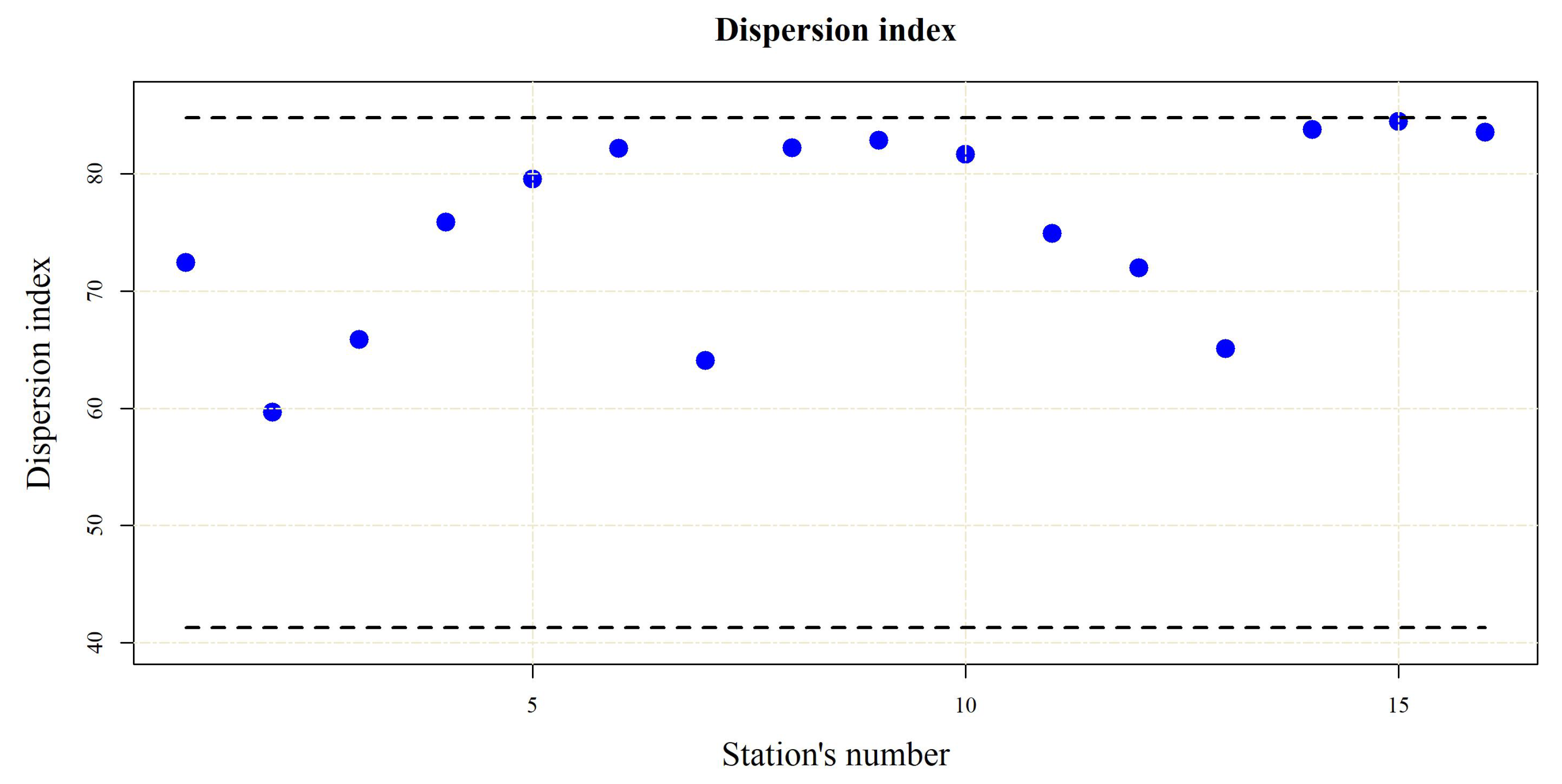
The values of the dispersion index $\psi$ varied from 59.66 to 84.44. All of the index values were within the 95% confidence interval (Figure 3). Therefore, it can be concluded that the distribution of the number of exceedances over threshold is Poisson and that the randomness of the POT events was confirmed.

3.1.3. The Anderson–Darling Test of Goodness of Fit

For each station, the ADU test statistic was lower than the critical value ADU${}_{\mathrm{crit}}$ (

Table 4. The design rainfall depths of return period T = 100 years and T = 200 years, and its $95\%$ confidence intervals.

Station	${\mathit{P}}_{\mathit{T}=100}$	${\mathit{CI}}_{{\mathit{P}}_{\mathit{T}=100}}$	${\mathit{P}}_{\mathit{T}=200}$	${\mathit{CI}}_{{\mathit{P}}_{\mathit{T}=200}}$
1. Raków	106.36	(82.06; 142.38)	128.14	(95.39; 178.56)
2. Sandomierz	120.95	(94.31; 158.27)	148.57	(112.33; 201.01)
3. Brynica	132.41	(104.02; 172.61)	161.98	(123.52; 218.19)
4. Wolbrom	124.62	(97.63; 163.78)	149.82	(113.61; 204.19)
5. Chrzanów	88.54	(79.27; 99.05)	96.14	(85.72; 107.09)
6. Tarnów	111.14	(99.05; 124.66)	121.44	(107.85; 136.63)
7. Pilzno	101.50	(89.94; 113.98)	110.72	(97.70; 124.78)
8. Rzeszów-Jasionka	79.85	(71.22; 89.45)	86.65	(76.91; 97.49)
9. Skoczów	171.88	(131.77; 228.23)	209.37	(154.99; 288.61)
10. Stróża	179.30	(138.73; 238.47)	222.26	(166.57; 306.31)
11. Nowy Sącz	91.27	(81.81; 101.73)	98.86	(88.19; 110.65)
12. Ochotnica Górna	159.67	(127.07; 203.82)	196.51	(152.23; 258.19)
13. Lesko	91.34	(75.56; 113.02)	103.60	(83.38; 132.17)
14. Wisłok Wielki	140.18	(112.20; 176.44	167.22	(130.12; 216.68)
15. Kasprowy Wierch	271.52	(211.75; 358.95)	333.97	(252.44; 457.28)
16. Cisna	119.74	(98.44; 147.69)	137.96	(110.45; 175.07)

). The conclusion can be drawn that for all stations the distribution of the rainfall depth over threshold is GPD.

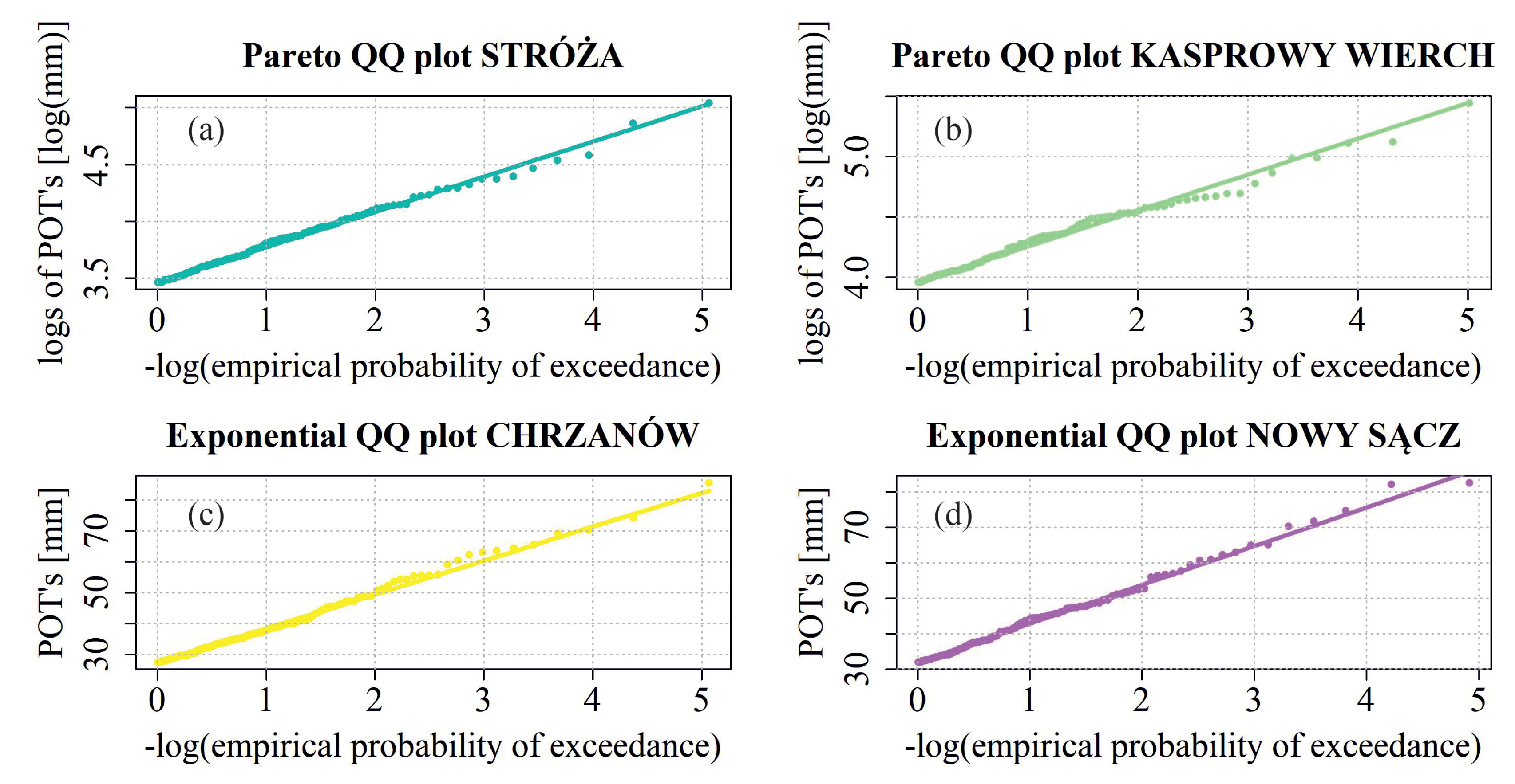
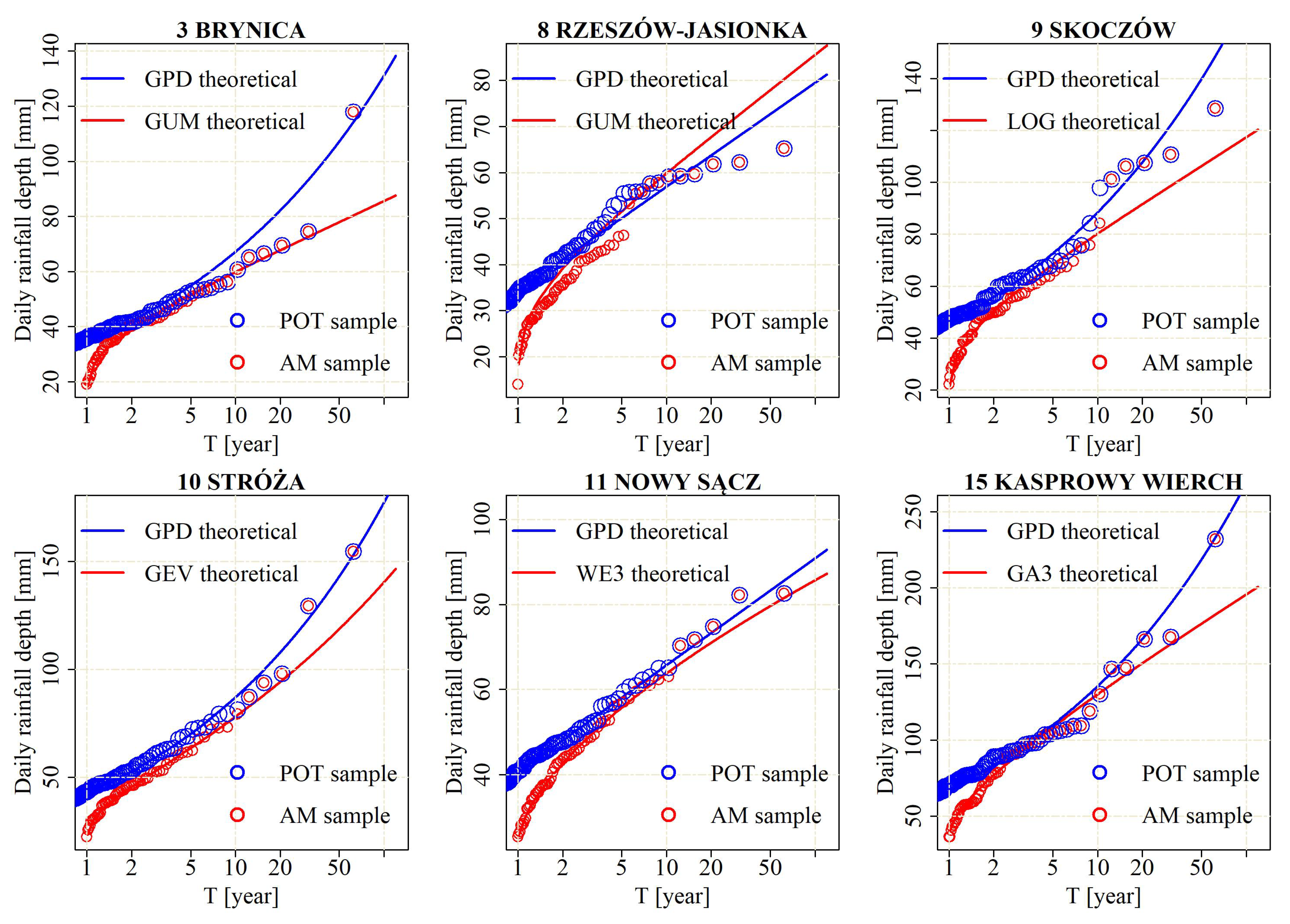
For 14 out of the 16 analysed stations, there is a good fit to the GPD or to the exponential distribution. However, in case of the Brynica and Rzeszów-Jasionka stations, the fit is weaker for higher precipitation values (the POT values are lower than the estimated values). The QQ plots for four exemplary stations (Stróża, Kasprowy Wierch, Chrzanów and Nowy Sącz) were shown in Figure 4. The congruence between the empirical and theoretical quantiles is evident in the plots, even for high rainfall depths.

3.1.4. The Design Rainfall Depth and Its Confidence Interval

For each station, the design rainfall depth was calculated from the Equation (8) for various return periods. The results for $T=100$ and $T=200$ years are presented in Table 4. For both of the return periods, the lowest values were obtained for the Rzeszów-Jasionka station, and the highest for the Kasprowy Wierch station. The $95\%$ confidence intervals of the design rainfalls were also shown in Table 4. They reflect uncertainty of design rainfall estimates.

The visual assessment of the CIs is easier on the lollipop charts (Figure 5) where $P_{T=100}$, and the lower and upper bounds of the CIs were depicted. A strong diversity and a high uncertainty of the estimated design rainfalls can be noted at Kasprowy Wierch, Stróża, and Skoczów stations where the CIs are widespread (see Figure 5). In the case of the Kasprowy Wierch station, the uncertainty is approximately at the level of 20%. The narrowest confidence intervals were obtained for Rzeszów-Jasionka, Chrzanów, Tarnów, Pilzno, and Nowy Sącz stations which show the lowest uncertainty of the estimated rainfalls at these stations. It can be noted that the stations with lower altitude have lower uncertainty of design rainfall than the stations with higher altitudes. Thus, the spatial properties of the UVB are reflected in the uncertainty of design rainfall.

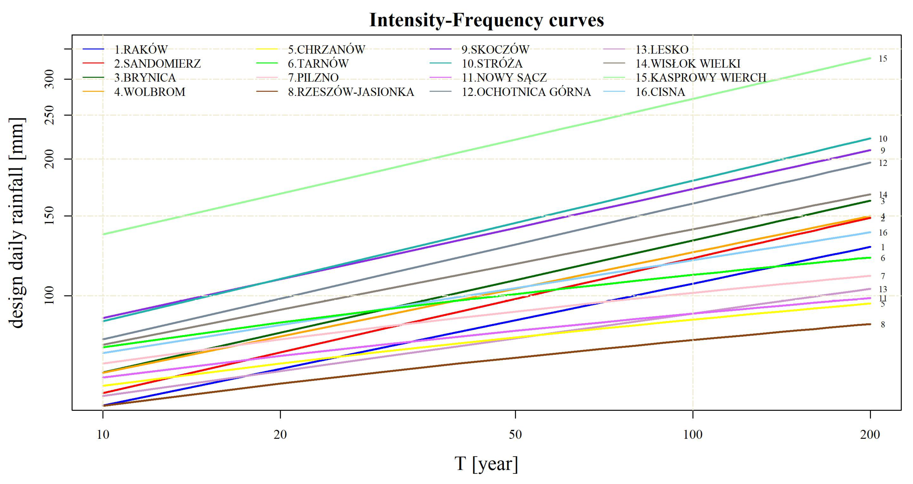
Figure 6 shows the intensity–frequency curves, where the dependence between design daily rainfall and recurrence period, as well as the comparison between design daily rainfalls for all stations, are depicted. For the Sandomierz (red line) and Raków (navy blue line) stations, in the case of short return periods ($T=10$ years), the design rainfall value is relatively low. However, as the return period increases, the rainfall also increases, and for $T=200$ years it exceeds 100 mm in both cases. The high values of the parameter $\gamma$ in the two stations are reflected in the strong increase of the intensity–requency curve. The lowest increase was obtained for the Tarnów, Chrzanów i Nowy Sącz stations, which in turn reflects a low value of the parameter $\gamma$. For all return periods $T\in [10,100]$, the highest values were obtained for the Kasprowy Wierch station. This station is located in the Carpathians (1991 m. a.s.l.). Meanwhile, the lowest values were found for Rzeszów-Jasionka, the station at the lowest altitude (200 m. a.s.l.). The issue of how the design rainfall depends on the altitude is discussed in detail in Section 3.4.

3.2. AM-Based Method

3.2.1. Selection AM Sample and Testing the Homogeneity

The verification was carried out by using the Mann–Kendall test, assuming the null hypothesis about the homogeneity of the data. The p-values of the MK test varied from $0.13$ to $1.0$. For the Wisłok Wielki station, the null hypothesis of no trend was rejected (increasing trend), and hence, because the homogeneity of the AM time series could not be confirmed, the station was omitted from further considerations. For the other 15 stations, the homogeneity of the AM series was confirmed.

3.2.2. Verification of the Type of the Distribution

The null hypothesis that the time series comes from a theoretical distribution F was verified by using the ADU test. For most stations, there were several distributions accepted by the test, e.g., the GEV, GA2, GA3, LOG, WE3, and GUM distributions. Therefore, as the hypothesis testing results were not conclusive enough in selecting the best fit, the AIC criterion was used in the next step.

3.2.3. Selection of the Best Distribution of the AM by Using the AIC Criterion

The AIC values were displayed in

Table 5. The AIC values for the GEV, GA2, GA3, LOG, WE2, WE3, and GUM distributions. The lowest AIC values (in boxes) show the distribution functions that provide the best fit.

Station	GEV	GA2	GA3	LOG	WE2	WE3	GUM
1. Raków	483.79	493.34	470.83	486.68	510.92	479.29	486.86
2. Sandomierz	496.87	507.19	488.86	498.82	527.11	503.14	499.39
3. Brynica	499.35	501.98	500.70	498.12	518.05	503.40	497.84
4. Wolbrom	509.04	508.94	508.90	507.14	517.54	509.70	507.13
5. Chrzanów	504.91	503.50	504.31	502.73	509.68	504.82	502.93
6. Tarnów	533.53	531.91	533.07	531.44	538.21	533.43	531.55
7. Pilzno	507.91	508.10	506.97	506.16	517.38	507.62	506.02
8. Rzeszów-Jasionka	483.19	481.69	483.48	481.67	487.11	485.27	481.66
9. Skoczów	541.56	544.23	542.15	540.52	555.86	544.30	540.66
10. Stróża	535.30	545.45	537.62	538.10	561.31	540.89	538.87
11. Nowy Sącz	494.12	494.73	491.73	492.74	504.25	490.52	492.26
12. Ochotnica Górna	525.93	540.82	532.97	531.81	558.98	539.42	531.65
13. Lesko	467.97	469.10	466.80	467.08	481.15	467.06	466.00
14. Wisłok Wielki	ne *	ne	ne	ne	ne	ne	ne
15. Kasprowy Wierch	602.26	605.08	576.67	601.08	616.41	601.40	602.18
16. Cisna	501.26	504.43	499.48	501.58	517.20	499.54	499.92

Note: * The distribution function of AM not estimated.

. The final choices, indicated by the lowest AIC values were marked with boxes. The conclusion can be drawn that the GEV distribution turned out to provide the best fit at two stations, GA3 at four stations, LOG at three stations, WE3 at one station, and GUM at five stations. The GA2 and WE3 were not selected for any station.

3.3. Selection of a Better Method from the POT and AM Based on the Comparison between Rainfall Depths Derived from the POT and AM Series

By using the Equation (8) and the return periods of 2, 5, 10, 12, 15, 20, 30, and 60 years (case 1) and 15, 20, 30, and 60 years (case 2), the design daily rainfall depths were derived from the GPD (POT-based method) and the theoretical distribution selected by using the AIC (AM-based method).

Figure 7 shows the design rainfall depths obtained from the GPD estimation (the POT-based method) and the GEV/GA3/LOG/WE3/GUM estimation (the AM-based method) for six exemplary stations. It can be observed that the GPD yields a better fit to high observed values than the AM-based fit (Brynica, Skoczów, Stróża, Nowy Sącz, Kasprowy Wierch). Many highest peaks were insufficiently designed with the AM-based method while the GPD fit was more accurate. A similar situation occurred in the other stations not shown here.

To quantify the efficiency of the POT method in comparison to the AM-based method, the RMSE and MDE criteria were used to measure the forecasting errors. The comparison was conducted by using the Equations (11) and (12). The results are shown in

Table 6. The scores $d_1,d_2$ assigned to the stations based on the comparison between the $\mathit{MDE}$ and $\mathit{RMSE}$ from the POT and AM methods. The number 1 shows a better fit. The final score d is shown under the table.

	Case 1				Case 2
Station	${\mathrm{MDE}}_{\mathrm{POT}}$	${\mathrm{MDE}}_{\mathrm{AM}}$	${\mathrm{RMSE}}_{\mathrm{POT}}$	${\mathrm{RMSE}}_{\mathrm{AM}}$	${\mathrm{MDE}}_{\mathrm{POT}}$	${\mathrm{MDE}}_{\mathrm{AM}}$	${\mathrm{RMSE}}_{\mathrm{POT}}$	${\mathrm{RMSE}}_{\mathrm{AM}}$
1. Raków	1	0	1	0	1	0	1	0
2. Sandomierz	1	0	1	0	1	0	1	0
3. Brynica	0	1	1	0	1	0	1	0
4. Wolbrom	1	0	0	1	0	1	0	1
5. Chrzanów	1	0	1	0	1	0	1	0
6. Tarnów	1	0	1	0	1	0	1	0
7. Pilzno	1	0	1	0	1	0	1	0
8. Rzeszów-J.	0	1	0	1	0	1	0	1
9. Skoczów	1	0	1	0	1	0	1	0
10. Stróża	1	0	1	0	1	0	1	0
11. Nowy Sącz	1	0	1	0	1	0	1	0
12. Ochotnica G.	1	0	1	0	1	0	1	0
13. Lesko	1	0	1	0	1	0	1	0
14. Wisłok Wielki	-	-	-	-	-	-	0	-
15. Kasprowy W.	1	0	1	0	1	0	1	0
16. Cisna	0	1	1	0	0	1	1	0
		d${}_{\mathrm{POT}}$ = 25	d${}_{\mathrm{AM}}$ = 5			d${}_{\mathrm{POT}}$ = 25	d${}_{\mathrm{AM}}$ = 5

.

In case 1, the final score d was 25 and 5 for the POT-based and AM-based method, respectively. Similarly, in case 2 the final score d was 25 to 5 in favor of the POT method.

It can be concluded that from the point of view of the RMSE and MDE criteria, a higher rating was given to the POT method. Hence, the POT method with Hill estimates of the GPD is a better choice in estimating daily precipitation totals in the UVB than the AM-based method.

3.4. Associations between Distribution Characteristics and Station’s Altitude

As evident in the results (Table 2), the parameters of the GPD differ between stations. Such differences can be also noted between design rainfall depths. Additionally, the difference is larger for longer return periods.

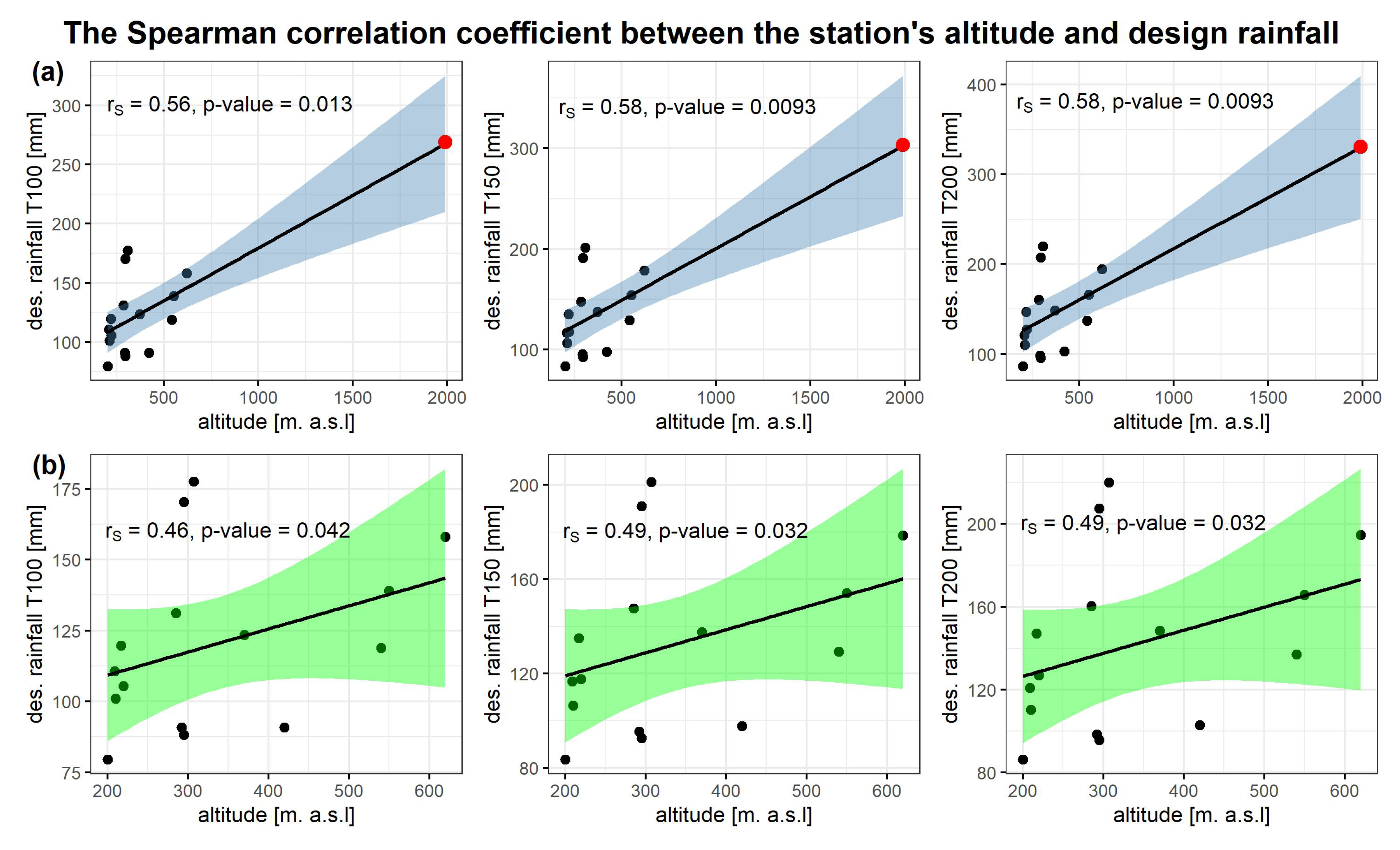
The sample Spearman correlation coefficient $r_S$ between the station’s altitude and design rainfall depth for return periods of 100, 150, and 200 years was calculated first. The scatterplots were shown in Figure 8. A deep insight into the sample values and in the scatterplot allows us to observe that after omitting the Kasprowy Wierch station (marked in red) the correlation becomes slightly weaker. As the Kasprowy Wierch station highly influences the relation, the two cases were considered next (a) with the Kasprowy Wierch and (b) without the Kasprowy Wierch station. The $r_S$ values varied from 0.56 to 0.58 in (a) and dropped to 0.46–0.49 in (b). The blue and green areas represent the confidence region around the regression line at the confidence level of $95\%$.

The question was if the dependence is strong in the whole region. It was confirmed, by using hypothesis testing, that ${\rho }_S$ is significantly greater than zero for return periods of 100, 150, and 200 years and in both cases (a) and (b). Thus, the positive relation between the height of the station and design rainfall depth was confirmed.

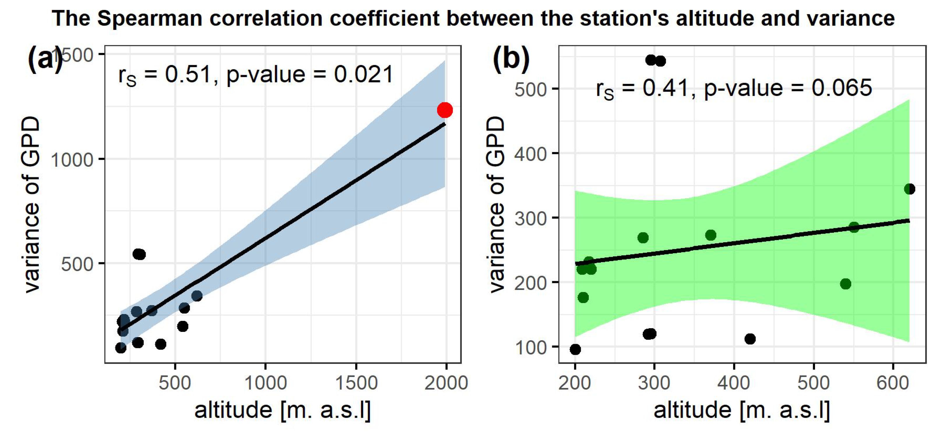
The sample correlation coefficient $r_S$ between the station’s altitude and the threshold $x_t$ equals 0.64 in (a) and 0.56 in (b) while between the station’s altitude and $Va{r}_{\mathrm{GPD}}$ equals 0.51 in (a) and 0.41 in (b) (see Figure 9). It was shown, by using hypothesis testing, that the correlation between the station’s altitude and both characteristics is significantly greater than zero.

The relation between the altitude and the $\gamma$ parameter values is also considerable because $\gamma$ is greater than zero at the stations with higher altitude (north and south of the UVB) and equal to zero at lower altitudes (central part of the UVB). The Spearman correlation coefficient equals $r_S=0.48$ (case (a)) and 0.39 (case (b)). The hypothesis testing for ${\rho }_S$ shows that it is significantly greater than zero in (a). However, in (b) the test failed to reject the null hypothesis of no correlation.

Remembering that the uncertainty of design rainfall depth was also associated with the station’s altitude (Section 3.1.4), this proves that the GPD properly reflects the increase in the magnitude and variability of design rainfall with the increase of each station’s altitude in the region.

The conclusion can be drawn that a strong spatial diversity can be ascribed to the GPD characteristics and to the predicted rainfalls with long return periods.

4. Discussion

To the best of our knowledge, this method has not been used in Poland so far. The novelty of the study was in the use of the Hill estimates of the GPD in a region in Poland that is very diverse with regard to rainfall pattern—ranging from moderate to torrential. The novelty also appiles to the assessment of the dependence between orography and characteristics of the GPD, which is important from the point of view of the precision of the estimates of high design rainfall totals. This is the first study in the UVB where the GPD with Hill estimates is adapted to the distribution of daily rainfall over threshold. Therefore, the comparison with other authors can be limited only to some aspects.

The drawback of all POT-based estimation methods is a lack of an unique, universal procedure of a threshold choice. However, basic guidelines that have been developed over the last several dozen years, should always be considered (see Introduction). The limitation of the POT-based method with Hill estimates is that the MSE-based optimal threshold, selected from the region of low fluctuation of $\widehat{\gamma }$, can be sometimes difficult to identify, and some experience is needed in analysing the relation between the MSE and potential thresholds. Nevertheless, the advantages of the POT-based method with the Hill estimates of the GPD, and its superiority over the AM-based method in the estimation of largest rainfall quantiles outweigh the disadvantages.

In [2,3,8], the POT method was also used for stations located in Poland. A detailed description of statistical tools and exemplary stations’ analysis was provided. However, it should be highlighted that the method of parameter estimation in [2,8] is MLE, which differs from the method used in this paper. Based only on plots in [8], as exact values were not provided there, it can be concluded that the design rainfalls computed by using the Hill statistics are somewhat higher than those obtained in [8].

A similar region (UVB) was studied by Młyński et al. [56], who chose GEV as the best distribution of the annual maximum precipitation, based on data (43 years) from 51 rainfall stations. The recommendation was based on various selection criteria (e.g., the peak-weighted root mean square error). In five stations that are common with five stations from this study, the $P_{T=10}$ values obtained by the authors [56] are similar to $P_{T=10}$ values estimated in this paper.

The results of Mascaro are similar to the results obtained in this paper with regard to the gamma parameter that was greater or equal to zero in various stations. However, the seasonal approach of the POT-based method with Hill statistics in the UVB might be considered in future plans.

Onyutha and Willems [26] derived the daily design rainfall in stations located in the Lake Victoria Basin by using the POT method and the GPD distribution and used various methods of estimation in terms of capturing the tail behaviour of the GPD and the uncertainty of the high-intensity quantiles. Some similarity between the results can be observed, namely the “normal tail” of the GPD ($\gamma$ near to zero) in all nine stations in [26] and only in five stations with relatively low altitude (200–300 m. a.s.l.) in this study. However, it should be stressed that $\gamma >0$ was estimated in a majority of stations in this study, in particular in all stations with altitude greater than 300 m. a.s.l. This confirms that the inclusion of the spatial factor in rainfall estimates in upland and mountainous areas was certified.

5. Conclusions

The estimation of design rainfalls for a wide range of return periods was carried out by using the POT-based method with the GPD distribution and the Hill estimates at 16 stations located in the UVB, a spatially diverse region vulnerable to flooding. The accurate estimation of the threshold, shape, and scale parameters of the GPD was shown to be a key point in the process because their values control the tail of the GPD.

After comparison between the results of the POT-based method (Hill estimates) with the AM-based method (MLE estimates + AIC), it was found that for 80% of the stations under study the priority should be given to the former method, which shows a very good performance of the POT-based method. The results show that the characteristics (threshold, variance) of the GPD vary between stations, increase with the station’s altitude, and that the shape parameter is greater than zero for stations located in the southern, mountainous part, and in the northern, upland region, while it is mostly equal to zero in the central part with a lower altitude. This highly influenced the values of the design rainfalls that increase with the station’s altitude. This indicates that orographic enhancement increased the design rainfall depth.

The conclusions can be drawn that the method is highly competitive with other methods in designing large rainfall events and that the GPD with Hill statistics is able to properly reflect the increase in the magnitude and variability of design rainfall with the increase in each station’s altitude in the region.

With regard to future plans, considering that only mountain and upland areas were studied, it would also be worthwhile to verify whether this method will accurately estimate high precipitation totals in lowland areas, characterized by a different precipitation pattern. The next issue is seasonality, which plays an important role in temporal rainfall scheme and thus should also be considered.

Therefore the method can be recommended in water-management applications related to floods in the UVB.