Two-Phase MPM Simulation of Surge Waves Generated by a Granular Landslide on an Erodible Slope

Abstract

A high-speed debris flow sliding into a reservoir can cause a huge disaster. Consequently, predicting landslide movement accurately and its potential interaction with water is crucial. This paper developed a computational model based on a two–layer two–phase material point method (MPM) to simulate surge waves generated by granular landslides on an erodible slope. By comparing granular landslide on a rigid and erodible slope, the effect of the slope erodibility on the process of landslide movement and the waves generated is investigated. The model takes full account of the large deformations, fluidisation and settlement of granular material in soil–water interactions. The numerical model is validated by comparing the simulated results with experimental data. The influences of internal friction angle, density, elastic modulus, Poisson ratio and dilatancy angle on wave height are also studied. The validated model was then used to investigate the surge waves generated by dry and saturated granules sliding along a rigid and erodible slope. The results show that both the erodible slope and saturated granular slide can increase the first wave crest height generated by the landslide.

1. Introduction

Debris flow is a mixture of granular materials and liquids, consisting of water, soil media and rocks that can slide downhill at high velocities [1]. Once it slips into a lake, bay or reservoir, it will produce a huge wave, which will have a major impact on the life and property safety of people, and even lead to catastrophic consequences [2]. Lituya Bay surge waves, 1958 [3,4] and surge waves caused by landslide of Vajont Reservoir in Italy, 1963 [5] are two well–known landslide surge waves events. Until now, the characteristics and movement processes of landslide–generated waves on slopes are still poorly understood, especially when it comes to slopes with different erosive properties, which makes it impossible to take effective measures to prevent the dangers posed by landslide generated water waves, and this has been an important issue that needs to be addressed worldwide. The behaviour of surge waves can vary significantly depending on the slope conditions on which the landslide is located and the near– and far–field geometry. Therefore, a comprehensive study of this complex phenomenon is essential to reduce the risk of landslide–generated surge waves.

In order to study the waves generated by landslides, researchers have developed various methods, in which the physical model test method [6] is more intuitive, but the test is more expensive and there is also a certain influence of the model scaling effect, which will have some influence on the results. Conversely, numerical simulation is widely used because of its unique advantages of low cost and the flexibility to be applied to almost any site configuration. Although the problem of surges caused by solid slides has been extensively studied since the 1970s, most landslides have been considered rigid materials in simulation studies of landslide–generated waves, ignoring their deformation effects [7,8,9,10,11]. In addition, to better understand the detailed movement of landslides, some scholars [12,13] employed two–fluid model to simulate the interaction between landslides and water. However, the movement of a landslide is different from that of a fluid, so this simplification does not accurately describe the movement and damage process of a landslide [14]. In order to bring the study closer to reality, the granular nature and deformable characteristics of the landslide should be considered [15,16]. In particular, it is important to accurately describe how granular materials enter water and the coupled granular–liquid interactions.

The numerical simulation of surges generated by granular bodies sliding along inclined surfaces is very difficult and challenging because it involves granular-liquid interactions, free surface flow, moving boundaries, large deformations, fluidisation and sedimentation of granular materials. Although mesh–based methods such as the finite element method (FEM) and the finite volume method (FVM) have been applied to study granular–liquid interaction problems and acceptable results have been obtained [16,17,18]. However, mesh–based methods require repeated updates to the computational mesh to track free-surface motion and large deformations, which becomes difficult and time–consuming. Alternative meshless methods such as smooth particle hydrodynamics (SPH) [19], material point method (MPM) [20], moving particle semi–implicit (MPS) method [21], lattice Boltzmann method (LBM) [22], and particle finite element methods (PFEM) [23], can simplify free surface tracking and make it easier to capture solid and liquid sloshing phenomena as the particles can move freely. Literatures [10,24,25,26,27,28,29] describe in detail the application of these particle methods to studying problems associated with landslide–generated water waves. Among the above mentioned meshless methods, MPM does not require a time–consuming search for neighbouring particles, but only the identification of particles relative to the background grid is needed, which is less computational, making MPM more promising for applications in the study of surges generated by sliding of granular bodies along differently eroded slopes. In this study, we used the two–layer two–phase MPM method [30] to investigate the phenomenon of landslides sliding along slopes with different erosion properties to produce surges, as this method provides a good description of pore water flow, the fluid–like behaviour of sand, and the change of state from free surface water to pore water, which is representative of sand fluidisation and sedimentation. Furthermore, the existing experimental and numerical studies have almost always used rigid slopes to study the phenomenon of landslide–generated water waves. However, in most real–world problems, slopes are erodible and landslides start sliding over bodies of water. An erodible slope has been found to increase the mobility of a landslide body [31,32]. Therefore, this paper focuses on the effect of erodible slope on the height of water wave generation.

The MPM [20] uses Lagrangian particles to track the deformation of the computational domain. However, unlike the previously mentioned particle methods, Eulerian background grids are used to solve the control equations. The combination of Eulerian and Lagrangian properties can overcome the problems of mesh distortion and interference with convective terms. Its background mesh is independent concerning the material domain and allows for an easier and more straightforward implementation of boundary conditions than other meshless methods such as SPH. Moreover, without the requirement for extra components, contacts between different entities may be determined automatically based on shared grid elements. Furthermore, the Mohr–Coulomb and Drucker–Prager models of landslide material composition are straightforward to include into MPM at the granular level. Large deformation issues may be modeled using the MPM technique, such as modeling landslides [33,34] and their interactions with reservoirs [35]. Therefore, the MPM method is more promising for studying large deformations in landslide–generated water waves.

This paper aims to demonstrate the feasibility of the proposed two–phase MPM method in simulating the surge wave generated by granular landslide along rigid and erodible slopes. The effects of sliding dry and saturated particles on the surge wave height on rigid and erodible slopes are also studied.

2. The Governing Equations

The two–layer two–phase MPM described here is based on the work of Abe et al. [36] and Bandara and Soga [37], in which the complicated solid–liquid coupling process is modeled with volume–fraction based mixture theory [38]. It assumes that each component of the mixture can be modeled as superimposing continuum medium so that each point in the solid–liquid mixture is occupied simultaneously by a material point of each constituent. As shown in Figure 1, the soil skeleton and the water phase are separately represented by two sets of material points, the dry soil material domain is only occupied by soil material points (SMPs), the free water domain is only occupied by water material points (WMPs), and the saturated soil is shared by WMPs and SMPs. Thus, the proposed two–layer two–phase MPM makes it possible to model the response of the dry soil, free water and saturated soil in an integrated framework. The unsaturated soil behavior is not considered in this paper. For the sake of brevity, we will present here only the governing equations, and the detailed description of the two–layer two–phase MPM can be found in the literature by Bandara and Soga [37]. The governing equations here are comprised of the mass conservation equations, the momentum conservation equations, and the material constitutive models.

2.1. Mass Balance Equations

Based on the mixture theory, the apparent density of soil and water in a soil–water mixture can be, respectively, expressed as

$${\overline{\rho }}_s=(1-n){\rho }_s$$

(1)

$${\overline{\rho }}_w=n{\rho }_w$$

(2)

where ${\rho }_s$ and ${\rho }_w$ are the intrinsic density of soil and water respectively, n is the soil porosity.

The mass balance equations for a unit volume of soil–water mixture consisting of soil and water phases can be written as follows:

$${\dot{\overline{\rho }}}_s+{\overline{\rho }}_s\left(\nabla \cdot v_s\right)=0$$

(3)

$${\dot{\overline{\rho }}}_w+{\overline{\rho }}_w\left(\nabla \cdot v_w\right)=0$$

(4)

where the superscript dot indicates time derivative. $v_s$ and $v_w$ are the velocity vectors of soil and water, respectively.

Substituting Equation (1) into Equation (3), neglecting the compressibility of soil grain and the gradient of density, the mass balance of the soil phase yields

$$\dot{n}=(1-n)\nabla \cdot v_s-v_s\nabla n$$

(5)

Substituting Equation (2) into Equation (4), using Equation (5), considering the compressibility of water phase and ignoring the density gradient, the water mass balance equation reduces to

$${\dot{\rho }}_w=-\frac{{\rho }_w}{n}[(1-n)\nabla \cdot v_s+n\nabla \cdot v_w+(v_w-v_s)\nabla n]$$

(6)

Assuming the water is weakly compressible fluid, the following equation is hold

$${\dot{\rho }}_w=\frac{{\rho }_w}{K_w}{\dot{p}}_w$$

(7)

where $K_w$ is the water bulk modulus and $p_w$ is the water pressure.

Substituting Equation (6) into Equation (7) yields

$${\dot{p}}_w=-\frac{K_w}{n}[(1-n)\nabla \cdot v_s+n\nabla \cdot v_w+(v_w-v_s)\nabla n]$$

(8)

It should be noted that Equation (8) is valid for the water both inside and outside the porous medium.

2.2. Momentum Balance Equations

Like the density, the apparent stresses of soil and water are defined respectively as:

$${\overline{\mathsf{\sigma }}}_s=(1-n){\mathsf{\sigma }}_s$$

(9)

$${\overline{\mathsf{\sigma }}}_w=n{\mathsf{\sigma }}_w$$

(10)

where ${\mathsf{\sigma }}_s$ and ${\mathsf{\sigma }}_w$ are the intrinsic stress tensor of soil and water phases respectively.

Based on the two–phase mixture theory, the behavior of water–saturated soil is determined by the interaction between soil skeleton and pore–fluid, each of which is regarded as a continuum that follows its own governing equations. The momentum equations of the soil and water phases are then written by

$${\overline{\rho }}_s{\dot{v}}_s=\nabla \cdot {\overline{\mathsf{\sigma }}}_s+{\overline{\rho }}_{s}g+f_{sw}$$

(11)

$${\overline{\rho }}_w{\dot{v}}_w=\nabla \cdot {\overline{\mathsf{\sigma }}}_w+{\overline{\rho }}_{w}g-f_{sw}$$

(12)

where g is the gravity acceleration vector, $f_{sw}$ is the force vector per unit volume due to soil–water interaction and can be defined by [39]

$$f_{sw}=f_d+{\mathsf{\sigma }}_w\nabla n$$

(13)

where the second term on the right hand of the equation is the ‘buoyancy force’ and the viscous drag force term $f_d$ will be discussed in the section of constitutive models.

Using the effective stress definitions, the apparent stress tensors of soil can be rewritten as

$${\overline{\mathsf{\sigma }}}_s={\mathsf{\sigma }}^{\prime }+(1-n){\mathsf{\sigma }}_w$$

(14)

where ${\mathsf{\sigma }}^{\prime }$ is the effective stress.

Substituting Equations (13) and (14) into Equations (11) and (12) yiel ds the final forms of momentum equations of the soil and water phases as follows:

$$(1-n){\rho }_s{\dot{v}}_s=\nabla \cdot {\mathsf{\sigma }}^{\prime }+(1-n)\nabla \cdot {\mathsf{\sigma }}_w+(1-n){\rho }_{s}g+{\mathsf{\sigma }}_w\nabla n+f_d$$

(15)

$$n{\rho }_w{\dot{v}}_w=n\nabla \cdot {\mathsf{\sigma }}_w+n{\rho }_{w}g-{\mathsf{\sigma }}_w\nabla n-f_d$$

(16)

2.3. Constitutive Models

In this paper, the water is treated as weakly compressible fluid with the stress computed by

$${\mathsf{\sigma }}_w=p_{w}I+2\mu {\dot{\mathsf{\epsilon }}}_w$$

(17)

where I is identity matrix, $\mu$ is the dynamic viscosity of water, and ${\dot{\mathsf{\epsilon }}}_w$ is the strain rate tensor. The pressure is updated using Equation (8), the strain rate is calculated by

$${\dot{\mathsf{\epsilon }}}_w=\nabla v_w+{\left(\nabla v_w\right)}^{\mathrm{T}}$$

(18)

For soil materials, the elastoplastic constitutive model with the Mohr–Coulomb yield criterion is applied. The effective stress is updated by

$$\dot{{\mathsf{\sigma }}^{\prime }}=D^e:\left(\dot{\mathsf{\epsilon }}-{\dot{\mathsf{\epsilon }}}^p\right)$$

(19)

where $D^e$ is the elastic stiffness tensor, $\dot{\mathsf{\epsilon }}$ is the strain rate tensor and ${\dot{\mathsf{\epsilon }}}^p$ is its plastic component that can be calculated using the plastic flow rule:

$${\dot{\mathsf{\epsilon }}}^p=\dot{\lambda }\frac{\partial g}{\partial {\mathsf{\sigma }}^{\prime }}$$

(20)

where $\dot{\lambda }$ is the rate of change of plastic multiplier and $g$ is the plastic potential function.

The yield function f for the Mohr–Coulomb yield criterion has the following form

$$f=\frac{1}{2}({{\mathsf{\sigma }}^{\prime }}_1-{{\mathsf{\sigma }}^{\prime }}_3)-\frac{1}{2}({{\mathsf{\sigma }}^{\prime }}_1+{{\mathsf{\sigma }}^{\prime }}_3)sin{\phi }^{\prime }+c^{\prime }cos{\phi }^{\prime }$$

(21)

where ${\phi }^{\prime }$ is the internal friction angle, $c^{\prime }$ is the cohesion. ${{\mathsf{\sigma }}^{\prime }}_1$, ${{\mathsf{\sigma }}^{\prime }}_2$, ${{\mathsf{\sigma }}^{\prime }}_3$ are the principal stresses where ${{\mathsf{\sigma }}^{\prime }}_1\le {{\mathsf{\sigma }}^{\prime }}_2\le {{\mathsf{\sigma }}^{\prime }}_3$ with assuming compressive stresses are negative.

The plastic potential function corresponding to a non–associated flow rule is used as follows

$$g=\frac{1}{2}\left({{\mathsf{\sigma }}^{\prime }}_1-{{\mathsf{\sigma }}^{\prime }}_3\right)-\frac{1}{2}\left({{\mathsf{\sigma }}^{\prime }}_1+{{\mathsf{\sigma }}^{\prime }}_3\right)\mathit{sin}\psi$$

(22)

where $\psi$ is the dilation angle.

Based on the works of Forchheimer [40] and Ergun [41], the drag force $f_d$ is determined in this paper by

$$f_d=\frac{n_{}^2\mu }{\kappa }(v_w-v_s)+\frac{1.75}{\sqrt{150\kappa }}{n}_{}^{1.5}{\rho }_w\left|v_w-v_s\right|(v_w-v_s)$$

(23)

where the soil permeability $\kappa$ is calculated using the following Kozeny–Karman formula:

$$\kappa =\frac{n_{}^3{D}_p^2}{150{\left(1-n\right)}^2}$$

(24)

where $D_p$ is the mean diameter of soil material.

It should be noted that the response of soil–water mixture may be changed from solid–like state to liquid–like state with the increasing of porosity and shear rate. This state change was characterized using a given maximum porosity n_max in this paper. When the porosity n is less than the maximum porosity n_max, the soil–water mixture behaves like a saturated soil and the foresaid elastoplastic constitutive model used to model the solid–like response. When the porosity n is beyond the maximum porosity n_max, the soil grains separate from each other and the effective stress vanished, the liquid–like behavior of soil–water mixture was modeled as weakly compressible fluid.

3. Numerical Examples

This section aims to validate the proposed two–phase MPM model and investigate the effect of dry and saturated granular bodies sliding along slopes with different erodibility to generate surges. MPM simulations were first carried out for topsoil erosion problems, followed immediately by simulated laboratory tests of dry particles sliding along sloping surfaces to generate surges to demonstrate the accuracy and effectiveness of the proposed method, and to investigate the effects of factors such as internal friction angle, density and expansion angle on surges. The validated two–phase MPM method was then applied to the study of the effects of surge generation from dry and saturated granular landslides sliding along rigid and erodible slopes.

3.1. Topsoil Erosion by Granular Landslides

In this subsection, the proposed two–phase MPM method is applied to the study of landslides sliding on erodible slopes and the numerical simulation results are compared with the results of laboratory tests conducted by Mangeney et al. [31]. In laboratory tests, granular landslides slide along a 22° slope under gravity (see Figure 2). The slope is 3 m long and 0.1 m wide. The width of the landslide is as wide as the flume and the slope has a layer of erodible slope with a thickness of 0.0046 m. The aspect ratio of the flume ensures that the landslide movement occurs in the x–direction, keeping the movement in a two–dimensional plane. Before the test began, a dry granular column was blocked to the left of the gate with an initial accumulation height of 0.14 m and a length of 0.2 m. When the gate was opened, the landslide began to collapse and slide.

This section uses the two–layer two–phase material point method to simulate the sliding of a deformable landslide along an erodible slope. The sliding process of the landslide at different moments and the distance of the granular body sliding along the wall and front are analyzed. The landslide was simulated using the Mohr–Coulomb model with the following material properties: elasticity modulus E = 2.0 × 10⁴ kPa, Poisson ratio ν = 0.3, granular density ${\rho }_s=1500$ kg/m³, average granular diameter D_p = 2 mm, internal friction angle ${\phi }^{\prime }$ = 25°, expansion angle $\psi$ = 0°, initial porosity n₀ = 0.3, cohesive force $c^{\prime }$ = 0 kPa. Similarly, the erodible slope was simulated using the Mohr–Coulomb intrinsic model with the following material properties: elasticity modulus E = 2.0 × 10⁴ kPa, Poisson ratio ν = 0.3, the density of granules on the slope ${\rho }_s$ = 1800 kg/m³, average granular diameter D_p = 2 mm, internal friction angle ${\phi }^{\prime }$ = 23°, expansion angle $\psi$ = 0°, initial porosity n₀ = 0.3, cohesive force $c^{\prime }$ = 3 kPa.

Figure 3a shows a schematic of the initial setup for the dry granular collapse simulation. The computational domain is divided into 37,200 tetrahedral cells with size of 0.01 m, as shown in Figure 3b. In order to reduce the computational cost, the model length was taken to be 2 m without affecting the results, and the model has only one cell in the thickness direction, with each element containing 4 solid phase material points, for a total of 75,789 material points. The horizontal displacement constraint is used to simulate the action of the gate, and the instantaneous release of the gate is achieved by lifting the horizontal displacement constraint. The time integration step used in this simulation is $1.205\times {10}^{-5}$ s and the total duration of the simulation is 1.0 s.

Figure 4 shows the snapshot for landslides sliding along erodible slopes at t = 0 s, 0.32 s and 0.64 s. The figure shows that as the granular material slides along the erodible slope surface, the slope surface also undergoes some deformation. The height and shape of the debris flow at different stages (t = 0 s, 0.32 s, and 0.64 s) are shown in Figure 5. The height of the debris flow was initially 0.14 m along the wall. At t = 0.32 s, the height along the wall fell to 0.125 m under gravity, and the front slid along the slope for 0.3 m. At t = 0.64 s, the height along the wall fell to about 0.08 m, and the front of the particles slid along the slope to about 0.9 m. The results show that the simulation results agree well with the results of the laboratory tests, indicating that the method is suitable for the simulation of soil–entrained debris flows.

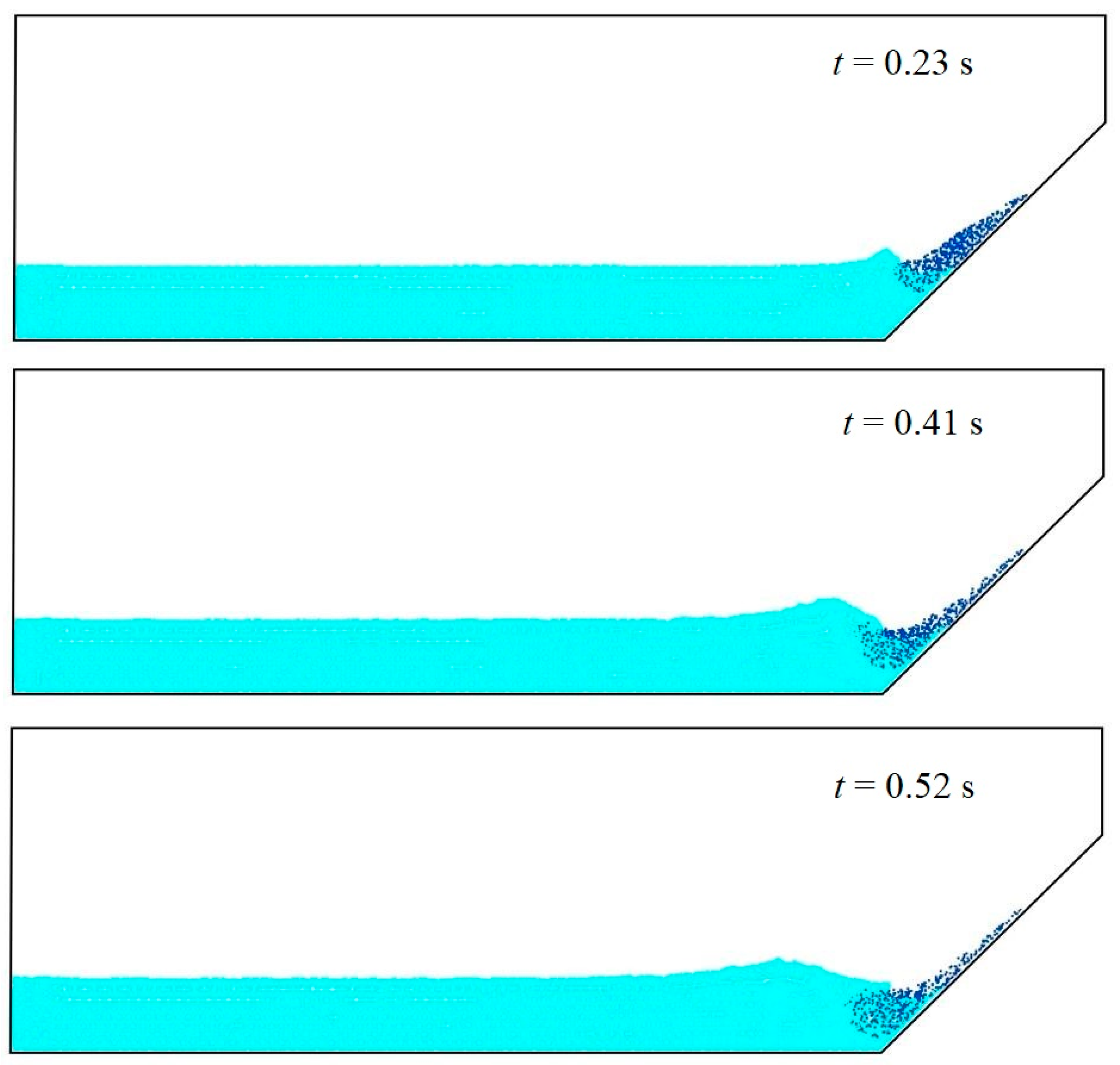
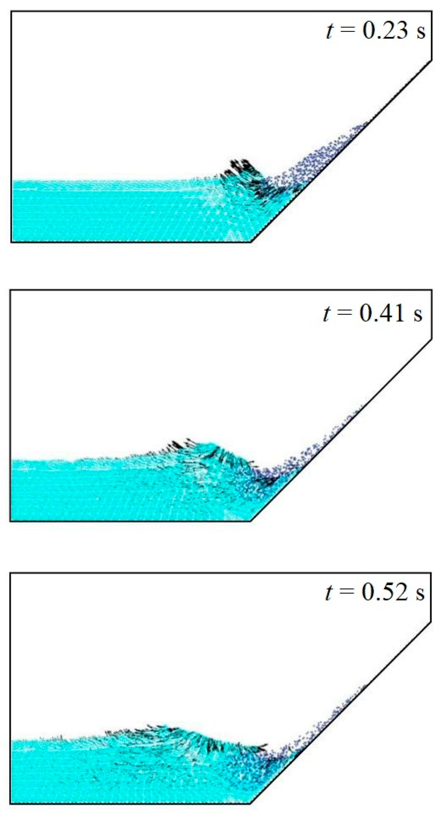
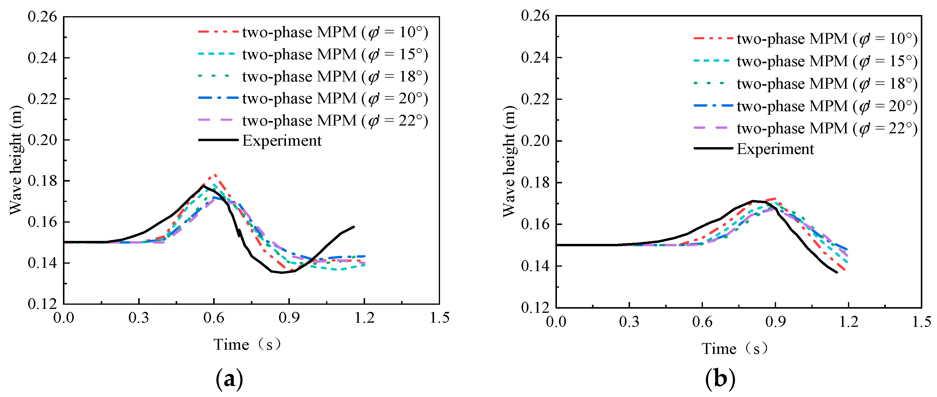
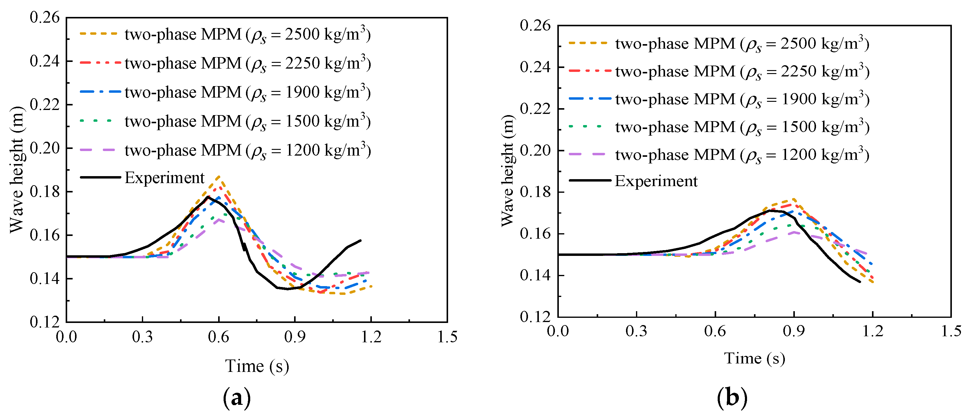
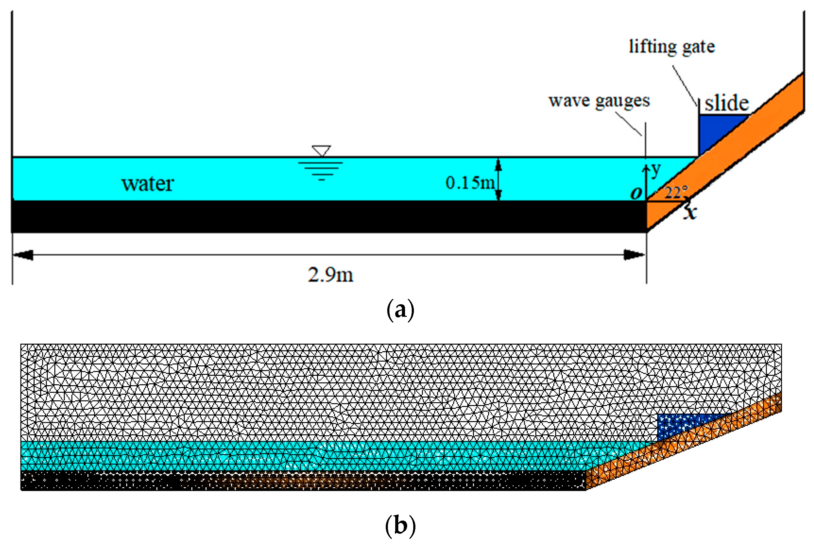
3.2. Surge Waves by Dry Granules Sliding on a Rigid Slope

In studies of landslide–generated wave problems, the problem is often further complicated when it involves particles coming into contact with and moving through a liquid, as the granular body interacts with the liquid and the presence of the surrounding liquid has an effect on the mobility of the sand [42]. This subsection presents a numerical simulation of a laboratory experiment carried out by Viroulet et al. [43] on wave generation by granular bodies entering water along a slope, verifying the process of dry particles sliding from a position above the water surface and generating waves, and performing a parametric sensitivity analysis. A schematic diagram of the experimental setup of Viroulet et al. [43,44] is shown in Figure 6a, with a slope inclination of 45°. The dry granular mass was held back by the gate before the start of the test in a 14.4 cm × 14.4 cm triangular pile–up pattern. The granular material used in the test is spherical glass beads, with the initial volume fraction a₀ = 0.6. The bottom of the device is filled with water, and the initial water depth h₀ = 15 cm. When the gate is opened, the granular body will begin to slide along the slope and fall into the water. The height of the wave generated by the granular body into the water is measured by a wave height meter at two different locations, they are 0.45 m and 0.75 m from the horizontal distance of the gate, respectively.

This section uses the two–layer two–phase MPM method to simulate the wave generation process of a dry granular body sliding into water along an inclined surface. The Mohr–Coulomb material model was used to simulate landslide properties with the following material properties: elasticity modulus E = 20,000 kPa, Poisson ratio $\mathsf{\nu }=0.3$, dry granular density ${\rho }_s$ = 2470 kg/m³, mean diameter D_p = 1.5 mm, internal friction angle ${\phi }^{\prime }$= 15°, expansion angle $\psi$ = 0°, initial porosity n₀ = 0.4. Water is considered to be a weakly compressible fluid with a material characteristic density of ${\rho }_w$ = 1000 kg/m³, a dynamic viscosity ${\mu }_w$ = 1.00 × 10⁻⁶ kPa·s and bulk modulus K_w = 2.15 × 10⁴ kPa.

Figure 6a is a schematic diagram of the initial form of the water wave model generated by dry particles sliding into water along the inclined plane. The test was approximated as a plane strain problem in the study, and the calculation area was divided into 26,148 tetrahedral grid elements of size 0.02 m, as shown in Figure 6b. There is only one element in the thickness direction of the model. Each dry granular body element contains 4 solid phase material points, each water element contains 4 liquid phase material points, and the model is surrounded by a fixed boundary with a total of 53,145 material points. The gates were opened instantaneously in the simulation, and the effect of instantaneous gate release was achieved by removing the restraint. The simulation uses a time increment of 2.517 × 10⁻⁵ s and a total duration of 1.2 s.

When the granular body slides into the water, as shown in Figure 7 (t = 0.23 s), due to the role of water resistance granular body front thickness increased, as the granular body along the slope gradually declined, the peripheral body of water along the direction of motion of the granular body was pushed forward, while the local water surface height increased, the water wave began to form.

In the simulation and prediction of landslide–generated water waves, the most important concern is often the characteristics of the leading wave (the first crest of a water wave) generated by the landslide, which is usually larger and more widespread than the second wave. Figure 8 shows the motion patterns of the granular body and the water column at different moments of time obtained from the numerical simulations. The arrows in the water column characterise the velocity of the water phase motion, the length of the arrow represents the velocity magnitude and the direction of the arrow represents the direction of the water column motion. As can be seen from the information on the velocity field distribution of the water column in Figure 8, the part of the water column in contact with the front of the granular body and the location of the water wave front has relatively large flow velocities.

Figure 9 shows the time evolution of the water surface height at two different locations (X1 = −0.3 m, X2 = −0.6 m) obtained by numerical calculation. The time at which the water waves reach their maximum crest is slightly delayed in the simulated results compared to the experimental results, which in combination with Figure 8 and Figure 9 is probably due to inaccurate modelling of the frontal morphology of the submerged granular body and the vortex of the water column. Considering the inherent complexity of the problem of water waves generated by landslides, the simulation results of the water wave propagation process in this section are generally acceptable, and the wave height of leading wave propagation to each observation point can be captured well.

In the two–layer two–phase MPM model proposed in this paper, the macroscopic intrinsic relationships of the granular body in the presence of the liquid phase are altered compared to dry particles, but the mathematical model of the relevant physical mechanisms is currently immature and empirical in nature. Thus, the impact of different material parameters on the initial amplitude of the water wave needs to be estimated. In addition, as the first wave characteristics generated by the landslide are the most influential in the simulation prediction of the actual landslide–generated water wave problem, only the correlation curve relationships between the different influencing parameters and the first wave are investigated in this section. Herein, the influence of internal friction angle, density, elastic modulus, Poisson ratio, and dilatancy angle of granular media on wave generation is analyzed.

The impact of internal friction angle of the sand is studied. Five internal friction angles (φ′ = 10°, 15°, 18°, 20°, and 22°) are considered in the simulation, and the other conditions remain unchanged. Figure 10 displays the change in free water surface height over time at locations X1 and X2 for the different internal friction angles. It shows that the impact of internal friction angle on the water wave is significant. The wave height decreases with increasing internal friction angle. Moreover, the crest height sharply decreases with increasing internal friction angle of sand.

Furthermore, the effect of sand density on the water wave is investigated. Five densities (ρ_s = 1200, 1500, 1900, 2250, and 2500 kg/m³) are used in the simulation, and other conditions remain unchanged. Figure 11 displays the change in free water surface height over time at locations X1 and X2 for different densities and displays the correlation of sand density. The numerical results show that the impact of density on the water wave is significant. The wave height increases with the density. Moreover, the crest height linearly increases with the sand density.

In addition, the effect of elasticity modulus of sliding sand is investigated. Five elasticity modulus (E = 5, 10, 20, 30, and 40 MPa) are used in the simulation, and other conditions remain unchanged. Figure 12 displays the change in free water surface height over time at locations X1 and X2 for different elasticity modulus and displays the correlation of elasticity modulus. The numerical results show that the impact of elasticity modulus on the water wave is almost negligible for slow landslides.

Additionally, the effect of Poisson ratio of sliding sand is investigated. Five Poisson ratios (ν = 0.1, 0.2, 0.25, 0.3, and 0.4) are used in the simulation, and other conditions remain unchanged. Figure 13 displays the change in free water surface height over time at locations X1 and X2 for different Poisson ratios and displays the correlation of Poisson ratio. The numerical results show that the impact of Poisson ratio on the water wave is almost negligible for slow landslides.

Finally, six dilatancy angles (ψ = 0°, 2°, 5°, 8°, 12°, and 15°) are used in the simulation, and the other conditions remain unchanged. Figure 14 displays the change in free water surface height over time at locations X1 and X2 for different dilatancy angles and displays the correlation of the dilatancy angle. The numerical results show that the effect of the dilatancy angle on water waves is almost negligible for slow landslides, which are investigated herein, this is consistent with the conclusions of Shi et al. [45].

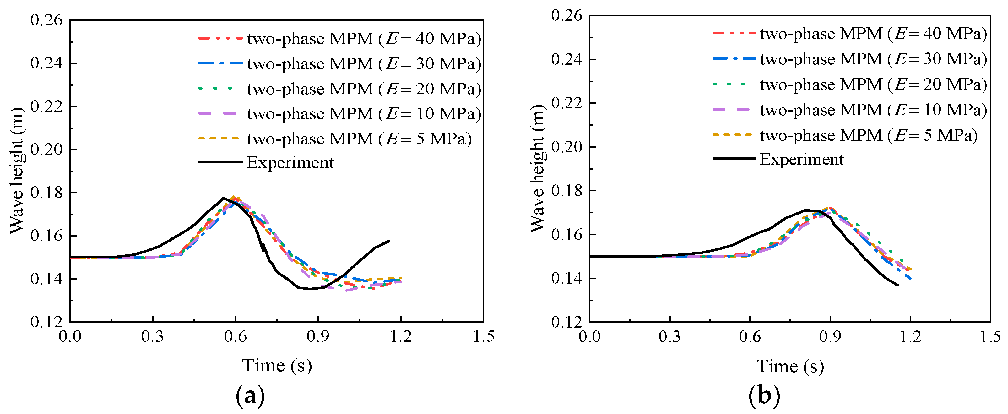
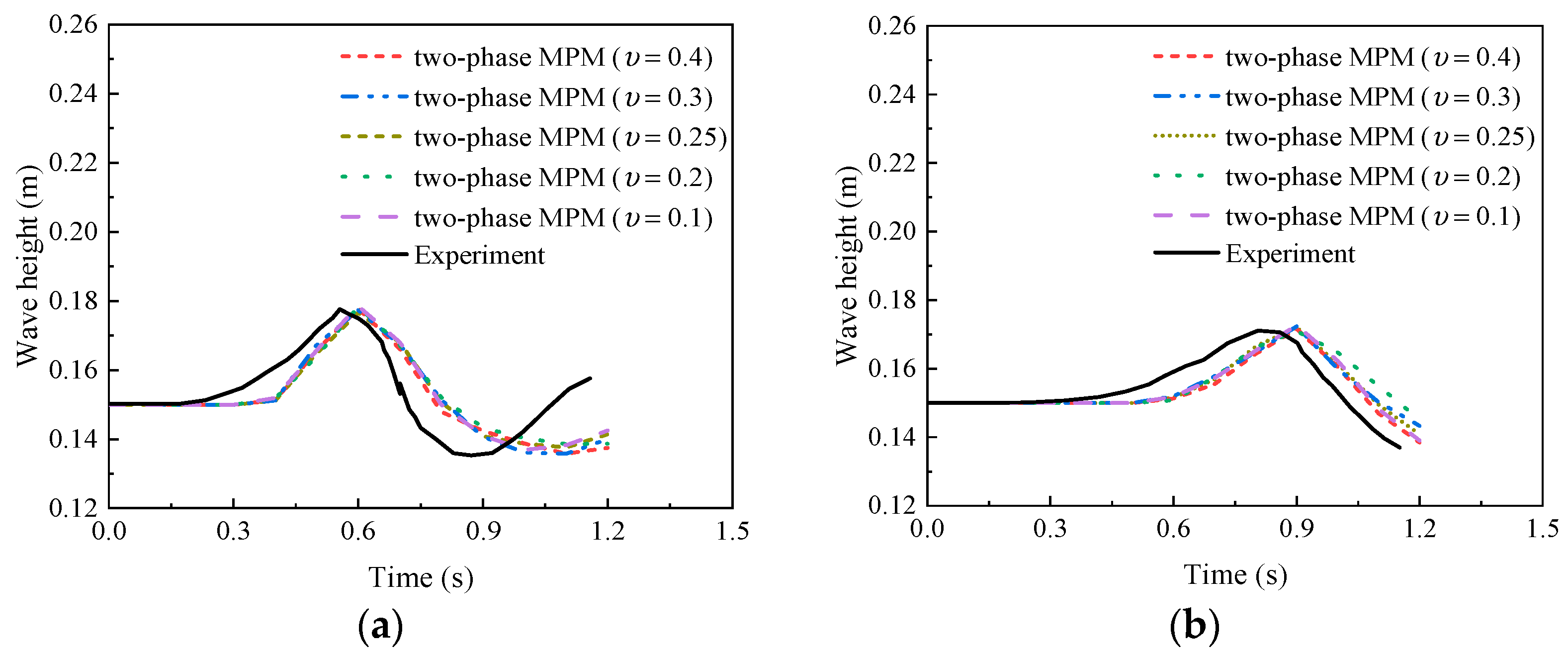
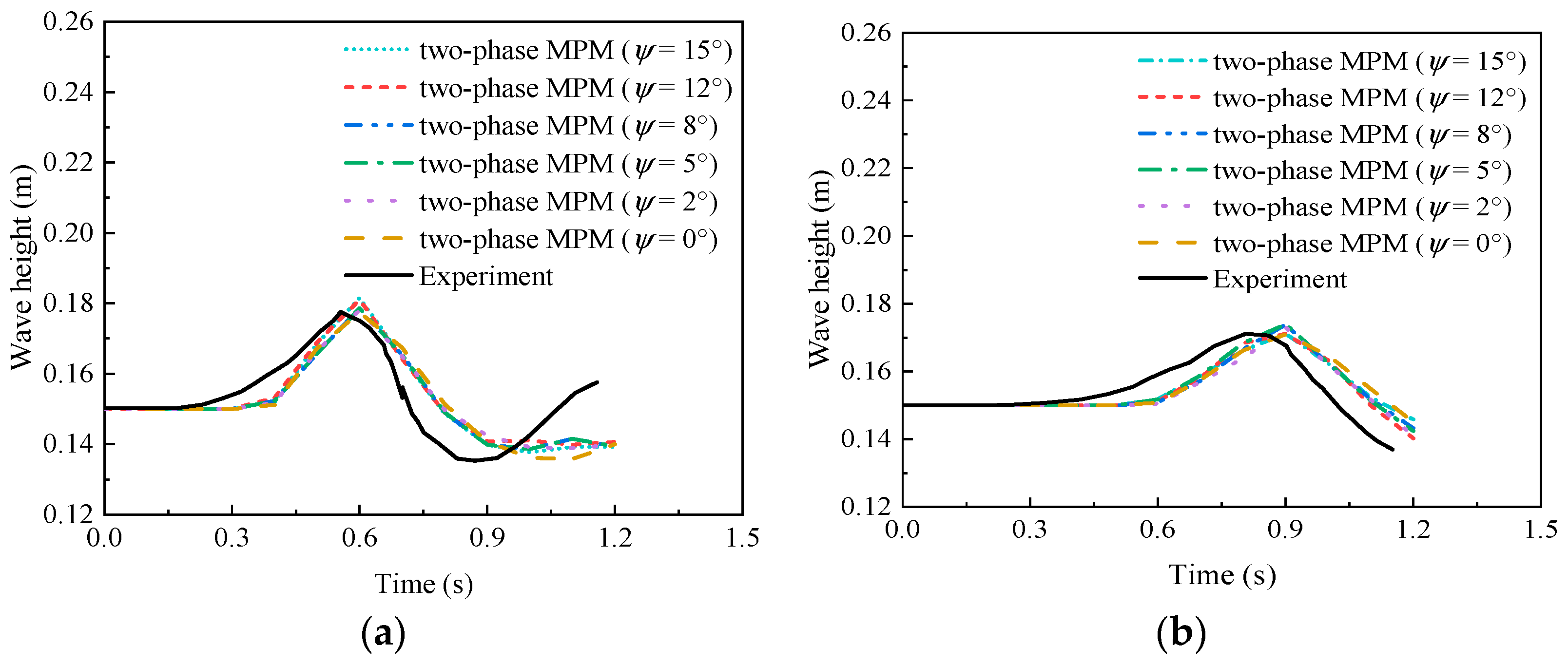
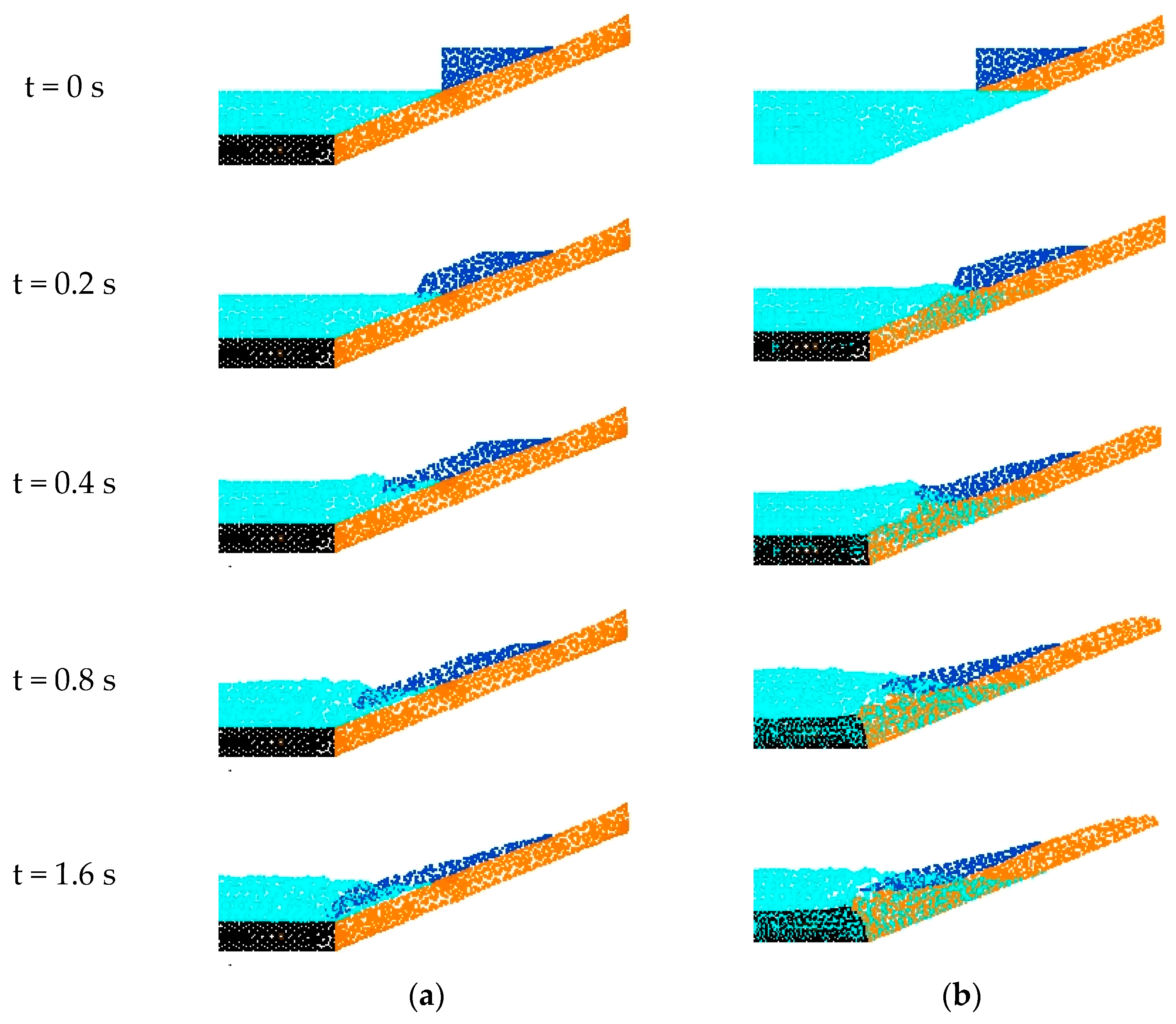
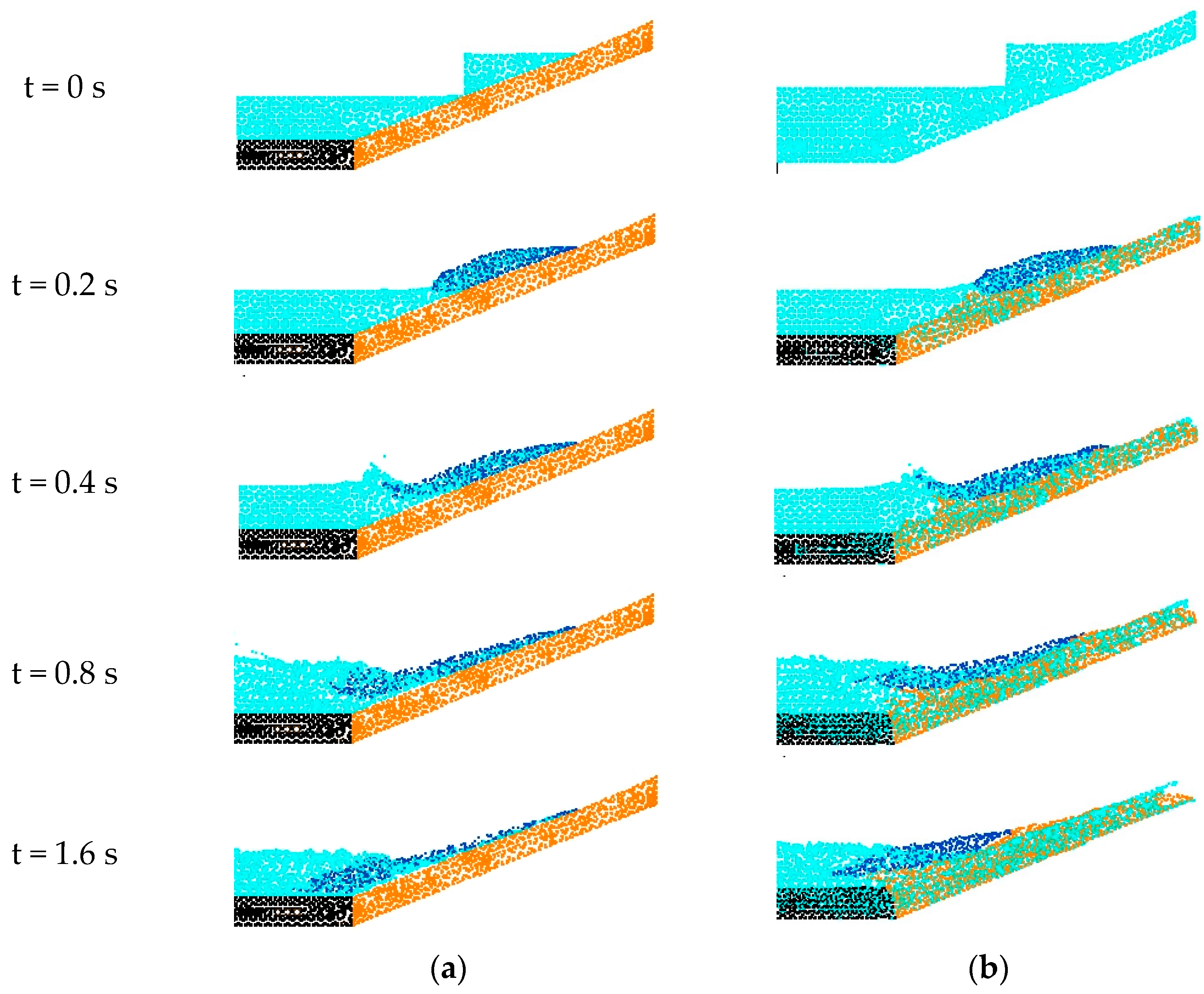
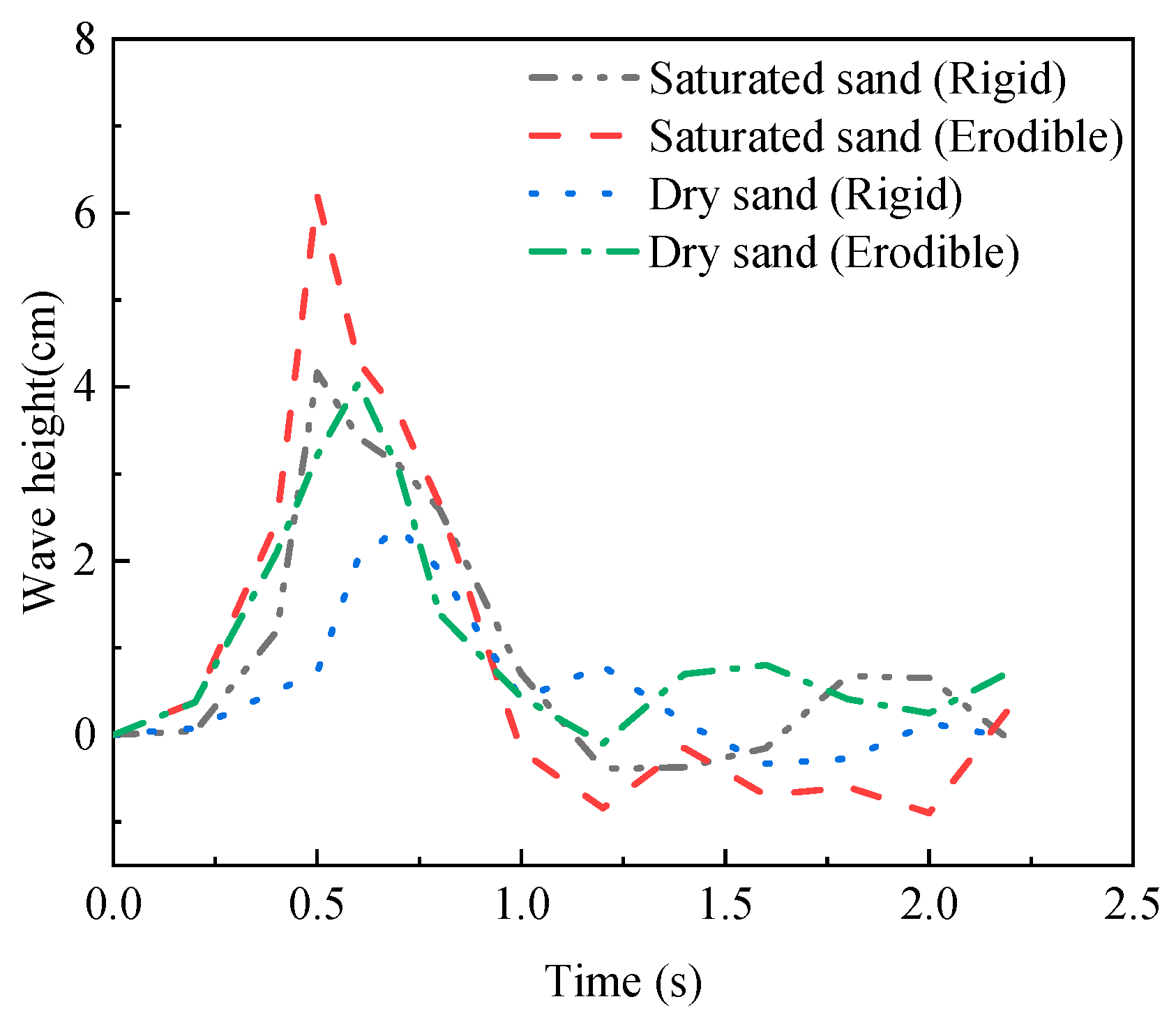
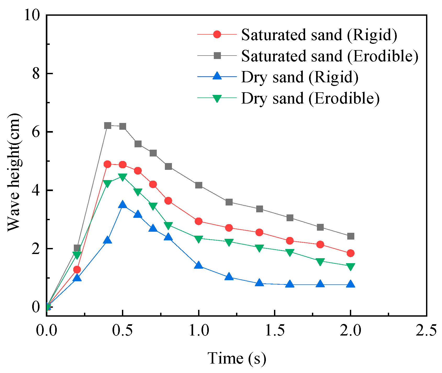
3.3. Surge Waves by Dry and Saturated Granules Sliding on Erodible Slope

In practice, most granular landslides have slopes that may not be rigid but erodible. Erodible slopes can increase the volume of granular slides compared to rigid slopes. This subsection uses a two–layer MPM approach to simulate the process of water waves generated by dry and saturated granular landslides sliding on rigid and erodible slopes, respectively. The critical parameters of the calculation model are summarised in

Table 1. Main parameters of the model.

Case	Slope Type	Elevation of Water Surface (m)	Tank Bottom Length (m)	The Dimensions of a Triangular Deposit (cm)	Slope Angle (°)
1	Rigid	0.15	2.9	14.4 × 38 (dry/saturated)	22
2	Erodible	0.15	2.9	14.4 × 38 (dry/saturated)	22

as Case 1 and Case 2. As shown in Figure 15a, the model is based on the experimental setup of Viroulet et al. [43], where the slope angle was adjusted to 22° to reduce the effect of the sliding of the slope itself. The effect of water waves generated by landslides on erodible slopes with dry granular and saturated particles is investigated by means of numerical calculation results for Case 1 and Case 2.

The material parameters used in the simulation of water waves generated by granular bodies sliding into water along different erosive slopes using the two–layer two–phase MPM method are shown in

Table 2. Material parameter.

Material	Parameter	Numerical Values
Landslides	Density (kg/m3)	1900
	Modulus of elasticity (kPa)	1.0 × 104
	Poisson ratio	0.3
	Internal friction angle (°)	15
	Expansion angle (°)	0
	Cohesion (kPa)	0
	Initial porosity	0.4
	Maximum porosity	0.5
	Mean diameter (mm)	2
Rigid slope	Density (kg/m3)	1900
	Modulus of elasticity (kPa)	1.0 × 104
	Poisson ratio	0.3
Erodible slope	Density (kg/m3)	1900
	Modulus of elasticity (kPa)	1.0 × 104
	Poisson ratio	0.3
	Expansion angle (°)	0
	Internal friction angle (°)	15
	Cohesion (kPa)	0.1
Water	Density (kg/m3)	1000
	Bulk modulus (kPa)	2.15 × 104
	Dynamic viscosity (kPa·s)	1.00 × 10−6

. The Mohr–Coulomb material model was used to simulate the properties of granular landslides as well as the properties of erodible slopes. Except for cohesion $c^{\prime }=0.1$ kPa, the erodible slope material properties are consistent with those of granular landslides. Rigid foundations are modelled using a linear elastic principal intrinsic model. Water is considered to be a weakly compressible fluid.

Figure 15a shows a schematic diagram of a computational model of a dry granular body sliding into water along an inclined plane to generate water waves. The test was approximated as a plane strain problem in the study, and the computational area was divided into 25,256 tetrahedral grid cells of size 0.02 m, as shown in Figure 15b. The model has only one element in the thickness direction, each dry granular body element contains 4 solid phase material points, each water element contains 4 liquid phase material points and the model is surrounded by a fixed boundary with a total of 34,868 material points. The gate is simulated using a horizontal displacement constraint and is released instantaneously by removing the constraint. The simulations used time increments of 2.517 × 10⁻⁵ s for a total duration of 2.2 s.

Figure 16 compares the characteristics of the temporal evolution of water waves generated by dry granular landslides along rigid versus erodible slopes. In general, for erodible slopes, the size of the active sliding area is much larger than for rigid slopes, resulting in higher heights of generated surges. At t = 0.2 s, the geometry of the sliding granules is less influenced by the erodibility of the slope. At t = 0.4 s, the granular body slides on the erodible slope with a slightly thicker and more deformed front, producing a slightly larger water wave. At t = 0.8 s, a portion of the granular body on the erodible slope is also deformed, causing a significant increase in the final thickness of the granular material deposited on the slope.

As shown in Figure 17, the time evolution of water waves generated by landslides along rigid versus erodible slopes is compared for saturated granular landslides. At t = 0.2 s, the granular body begins to drive the granular body surface of the slope as it slides on the erodible slope. The ensuing sliding process drove more and more of the slope surface together and created larger waves. Relative to the dry particle sliding shape in Figure 16, at the same moment, the saturated granular body deforms more during the sliding process and produces a higher height of water waves.

The variation of wave height with time at the location of the measurement point (X = 0 m) for Case 1 and Case 2 is shown in Figure 18. It can be seen that the wave amplitude caused by the sliding of granular bodies on erodible slopes is greater relative to that when sliding on rigid slopes, for both dry and saturated granular body landslides. For the same slope conditions, the water wave heights generated by a landslide of saturated granular bodies are greater than those generated by dry granular bodies.

Figure 19 shows the course of the leading wave heights produced by dry and saturated granular bodies over time for both rigid slope and erodible slope surfaces. Overall, the maximum values of the leading wave heights in the four cases occur at approximately 0.4–0.5 s, and the leading wave heights generated when the granular body slides along an erodible slope during sliding are found to be higher than on rigid slopes. At t ≈ 0.5 s, the height of the first wave for the erodible slope is about 27.5% higher than that for the rigid slope for dry sand (for dry sand or saturated sand). When slope conditions are the same, the leading wave generated by sliding saturated granules is higher than the leading wave generated by dry granules. After reaching its maximum height, the first wave decreases its height as the wave propagates.

In summary, we find that landslides in saturated conditions and along erodible slopes produce higher surge heights and greater hazards. Conversely, the wave height generated when sliding along a rigid slope in the dry granular condition is much smaller, and the risk factor is lower.

4. Conclusions

This paper proposes a two–phase MPM based on a two–layer formulation to simulate the granular-fluid interactions, free–surface flow, wave breaking, large deformation, and the granular fluidisation and sedimentation processes involved in the surge wave generation by granular landslides along rigid and erodible slopes.

The validation of the feasibility and applicability of the two–phase MPM through examples of topsoil erosion problems and aerial granular landslides generated surges, and finds that wave height decreases at higher internal friction angles, increases at higher densities and is less affected by Poisson ratio, modulus of elasticity and angle of expansion. Subsequently, the effect of sliding of dry and saturated granular bodies along rigid and erodible slopes on the height and first wave amplitude of the generated waves was investigated. The numerical results show that the granular body causes the volume of the landslide to increase as it slides along the erodible slope, which leads to the generation of higher surge waves and the greater amplitude of the leading waves. It was also found that saturated granular bodies sliding produced higher surges and greater leading wave amplitudes than dry granular bodies sliding. The results of these numerical studies implied that surge waves generated by debris flows are more dangerous than those generated by dry granular, and that debris flows sliding along erodible slopes are more dangerous than surge waves generated by sliding along rigid slopes because their waves are large and fast and can have a devastating impact on the environment and society.

In summary, the proposed two–layer two–phase MPM is a promising numerical tool for simulating the sliding of granular bodies along slopes with different erodibility and generating surge waves. However, due to the high computational cost, practical engineering simulations require a fast, inexpensive and scalable hardware acceleration technique.

References

1. Iverson, R.M. The physics of debris flows. J. Rev. Geophys. 1997, 35, 245–296. [Google Scholar] [CrossRef] [Green Version]
2. Evans, S.G. The 1946 Mount Colonel Foster rock avalanche and associated displacement wave, Vancouver Island, British Columbia. Can. Geotech. J. 1989, 26, 447–452. [Google Scholar] [CrossRef]
3. Miller, D.J. Giant waves in Lituya Bay, Alaska. J. Geophys. Res. 1959, 64, 692. [Google Scholar] [CrossRef]
4. Fritz, H.M.; Hager, W.H.; Minor, H. Lituya Bay case; rockslide impact and wave run-up. Sci. Tsunami Hazards 2001, 19, 3–22. [Google Scholar]
5. Alonso, E.E.; Pinyol, N.M. Criteria for rapid sliding I. A review of Vaiont case. Eng. Geol. 2010, 114, 198–210. [Google Scholar] [CrossRef] [Green Version]
6. Chen, L.; Wang, P.Y.; Yu, T.; Zhang, F.; Men, Y.Q. Model test research on soil-landslide surge by river channel reservoir. Appl. Mech. Mater. 2013, 353–356, 2610–2613. [Google Scholar] [CrossRef]
7. Wang, R.; Ding, M.; Wang, Y.; Xu, W.; Yan, L. Field characterization of landslide-induced surge waves based on computational fluid dynamics. Front. Physics. 2022, 9, 1–11. [Google Scholar] [CrossRef]
8. Viroulet, S.; Cebron, D.; Kimmoun, O.; Kharif, C. Shallow water waves generated by subaerial solid landslides. Geophys. J. Int. 2013, 193, 747–762. [Google Scholar] [CrossRef] [Green Version]
9. Jin, Y.C.; Guo, K.; Tai, Y.C.; Lu, C.H. Laboratory and numerical study of the flow field of subaqueous block sliding on a slope. Ocean Eng. 2016, 124, 371–383. [Google Scholar] [CrossRef]
10. Qiu, L.; Tian, L.; Liu, X.; Han, Y. A 3D multiple-relaxation-time LBM for modeling landslide-induced surge waves. Eng. Anal. Bound. Elem. 2019, 102, 51–59. [Google Scholar] [CrossRef]
11. Lynett, P.; Liu, P. A numerical study of the run-up generated by three-dimensional landslides. J. Geophys. Res.-Oceans 2005, 110, 1–16. [Google Scholar] [CrossRef] [Green Version]
12. Basu, D.; Das, K.; Green, S.; Janetzke, R.; Stamatakos, J. Numerical simulation of surface waves generated by a subaerial landslide at Lituya Bay Alaska. J. Offshore Mech. Arct. Eng. Trans. ASME 2010, 132, 041101. [Google Scholar] [CrossRef] [Green Version]
13. Cremonesi, M.; Frangi, A.; Perego, U. A lagrangian finite element approach for the simulation of water-waves induced by landslides. Comput. Struct. 2011, 89, 1086–1093. [Google Scholar] [CrossRef]
14. Xu, W.J.; Dong, X.Y. Simulation and verification of landslide tsunamis using a 3D SPH-DEM coupling method. Comput. Geotech. 2021, 129, 103803. [Google Scholar] [CrossRef]
15. Xue, H.C.; Ma, Q.; Diao, M.J.; Jiang, L. Propagation characteristics of subaerial landslide-generated impulse waves. Environ. Fluid Mech. 2019, 19, 203–230. [Google Scholar] [CrossRef]
16. Si, P.F.; Shi, H.B.; Yu, X.P. A general numerical model for surface waves generated by granular material intruding into a water body. Coast. Eng. 2018, 142, 42–51. [Google Scholar] [CrossRef]
17. Rzadkiewicz, S.A.; Mariotti, C.; Heinrich, P. Numerical simulation of submarine landslides and their hydraulic effects. J. Waterw. Port Coast. Ocean. Eng.-ASCE 1997, 123, 149–157. [Google Scholar] [CrossRef]
18. Zhao, L.; You, G. Rainfall affected stability analysis of maddingley brown coal eastern batter using plaxis 3D. Arab. J. Geosci. 2020, 13, 1071. [Google Scholar] [CrossRef]
19. Gingold, R.A.; Monaghan, J.J. Smoothed particle hydrodynamics: Theory and applications to non-spherical stars. Mon. Not. R. Astron. Soc. 1977, 181, 375–389. [Google Scholar] [CrossRef]
20. Sulsky, D.; Chen, Z.; Schreyer, H.L. A particle method for history-dependent materials. Comput. Meth. Appl. Mech. Eng. 1994, 118, 179–196. [Google Scholar] [CrossRef]
21. Koshizuka, S.; Oka, Y. Moving-particle semi-implicit method for fragmentation of incompressible fluid. Nucl. Sci. Eng. 1996, 123, 421–434. [Google Scholar] [CrossRef]
22. Chen, S.; Doolen, G.D. Lattice boltzmann method for fluid flows. Annu. Rev. Fluid Mech. 1998, 30, 329–364. [Google Scholar] [CrossRef] [Green Version]
23. Idelsohn, S.R.; Onate, E.; Del Pin, F. The particle finite element method: A powerful tool to solve incompressible flows with free-surfaces and breaking waves. Int. J. Numer. Methods Eng. 2004, 61, 964–989. [Google Scholar] [CrossRef] [Green Version]
24. Jin, Y.F.; Yin, Z.Y.; Zhou, X.W.; Liu, F.T. A stable node-based smoothed PFEM for solving geotechnical large deformation 2d problems. Comput. Meth. Appl. Mech. Eng. 2021, 387, 114179. [Google Scholar] [CrossRef]
25. Fu, L.; Jin, Y.C. Investigation of non-deformable and deformable landslides using meshfree method. Ocean Eng. 2015, 109, 192–206. [Google Scholar] [CrossRef]
26. Qi, Y.T.; Chen, J.Y.; Zhang, G.B.; Xu, Q.; Li, J. An improved multi-phase weakly-compressible SPH model for modeling various landslides. Powder Technol. 2022, 397, 117120. [Google Scholar] [CrossRef]
27. Qiu, L.C.; Jin, F.; Lin, P.Z.; Liu, Y.; Han, Y. Numerical simulation of submarine landslide tsunamis using particle based methods. J. Hydrodyn. 2017, 29, 542–551. [Google Scholar] [CrossRef]
28. Zhao, K.L.; Qiu, L.C.; Liu, Y. Two-layer two-phase material point method simulation of granular landslides and generated tsunami waves. Phys. Fluids 2022, 34, 123312. [Google Scholar] [CrossRef]
29. Nabian, M.A.; Farhadi, L. Multiphase mesh-free particle method for simulating granular flows and sediment transport. J. Hydraul. Eng. 2017, 143. [Google Scholar] [CrossRef]
30. Bandara, S.; Soga, K. Coupling of soil deformation and pore fluid flow using material point method. Comput. Geotech. 2015, 63, 199–214. [Google Scholar] [CrossRef]
31. Mangeney, A.; Roche, O.; Hungr, O.; Mangold, N.; Faccanoni, G.; Lucas, A. Erosion and mobility in granular collapse over sloping beds. J. Geophys. Res.-Earth Surf. 2010, 115. [Google Scholar] [CrossRef] [Green Version]
32. Mangeney, A.; Tsimring, L.S.; Volfson, D.; Aranson, I.S.; Bouchut, F. Avalanche mobility induced by the presence of an erodible bed and associated entrainment. Geophys. Res. Lett. 2007, 34. [Google Scholar] [CrossRef] [Green Version]
33. Yerro, A.; Soga, K.; Bray, J. Runout evaluation of oso landslide with the material point method. Can. Geotech. J. 2019, 56, 1304–1317. [Google Scholar] [CrossRef] [Green Version]
34. Soga, K.; Alonso, E.; Yerro, A.; Kumar, K.; Bandara, S. Trends in large-deformation analysis of landslide mass movements with particular emphasis on the material point method. Geotechnique. 2016, 66, 248–273. [Google Scholar] [CrossRef] [Green Version]
35. Du, W.J.; Sheng, Q.; Fu, X.D.; Chen, J.; Zhou, Y.Q. Extensions of the two-phase double-point material point method to simulate the landslide-induced surge process. Eng. Anal. Bound. Elem. 2021, 133, 362–375. [Google Scholar] [CrossRef]
36. Abe, K.; Soga, K.; Bandara, S. Material point method for coupled hydromechanical problems. J. Geotech. Geoenviron. Eng. 2014, 140. [Google Scholar] [CrossRef]
37. Bandara, S.; Soga, K. Coupling of soil deformation and pore fluid flow using material point method. Comput. Geotech. 2015, 65, 302. [Google Scholar] [CrossRef]
38. Truesdell, C.; Toupin, R. The classical field theories. In Handbuch der Physik; Springer: Berlin/Heidelberg, Germany, 1960; Volume 2. [Google Scholar]
39. Vardoulakis, I. Fluidisation in artesian flow conditions: Hydromechanically stable granular media. Geotechnique 2004, 54, 117–130. [Google Scholar] [CrossRef]
40. Forchheimer, P. Wasserbewegung durch boden. Z. Ver. Dtsch. Ing. 1901, 45, 1782–1788. [Google Scholar]
41. Ergun, S. Fluid flow through packed columns. J. Mater. Sci. Chem. Eng. 1952, 48, 89–94. [Google Scholar]
42. Topin, V.; Monerie, Y.; Perales, F.; Radjai, F. Collapse dynamics and runout of dense granular materials in a fluid. Phys. Rev. Lett. 2012, 109, 188001. [Google Scholar] [CrossRef] [PubMed] [Green Version]
43. Viroulet, S.; Sauret, A.; Kimmoun, O.; Kharif, C. Granular collapse into water: Toward tsunami landslides. J. Vis. 2013, 16, 189–191. [Google Scholar] [CrossRef]
44. Viroulet, S.; Sauret, A.; Kimmoun, O. Tsunami generated by a granular collapse down a rough inclined plane. EPL-Europhys Lett. 2014, 105, 34004. [Google Scholar] [CrossRef] [Green Version]
45. Shi, C.Q.; An, Y.; Wu, Q.; Liu, Q.Q.; Cao, Z.X. Numerical simulation of landslide-generated waves using a soil-water coupling smoothed particle hydrodynamics model. Adv. Water Resour. 2016, 92, 130–141. [Google Scholar] [CrossRef] [Green Version]
Figure 1. Diagram of the two–phase MPM based on the mixture theory.
Water 15 01307 g001
Figure 2. Diagram of the test setup.
Water 15 01307 g002
Figure 3. Computational model of a granular landslide sliding along an erodible slope: (a) Schematic of the initial model; (b) MPM discretization.
Water 15 01307 g003
Figure 4. Snapshots for landslides sliding along erodible slopes.
Water 15 01307 g004
Figure 5. Thickness profile comparison of experimental and numerical results.
Water 15 01307 g005
Figure 6. Calculation model for wave generation from dry granules into water along a slope: (a) Diagram of the initial form; (b) MPM discretization.
Water 15 01307 g006
Figure 7. Morphology of water waves generated by dry granular bodies entering the water at different moments.
Water 15 01307 g007
Figure 8. Simulation results of waves generated when particles enter water along a slope.
Water 15 01307 g008
Figure 9. Comparison of wave height test results with numerical results at two different locations: (a) X1 = −0.3 m; (b) X2 = −0.6 m.
Water 15 01307 g009
Figure 10. Influence of internal friction angle of sliding sand: time history curve of the free water surface at two different locations: (a) X1 = −0.3 m; (b) X2 = −0.6 m.
Water 15 01307 g010
Figure 11. Influence of density of sliding sand: time history curve of the free water surface at two different locations: (a) X1 = −0.3 m; (b) X2 = −0.6 m.
Water 15 01307 g011
Figure 12. Influence of elasticity modulus of sliding sand: time history curve of the free water surface at two different locations: (a) X1 = −0.3 m; (b) X2 = −0.6 m.
Water 15 01307 g012
Figure 13. Influence of Poisson ratio of sliding sand: time history curve of the free water surface at two different locations: (a) X1 = −0.3 m; (b) X2 = −0.6 m.
Water 15 01307 g013
Figure 14. Influence of dilatancy angle of sliding sand: time history curve of the free water surface at two different locations: (a) X1 = −0.3 m; (b) X2 = −0.6 m.
Water 15 01307 g014
Figure 15. Schematic diagram of a computational model for water waves generated by dry particles sliding along a rigid slope: (a) Schematic of the initial model; (b) MPM discretization.
Water 15 01307 g015
Figure 16. Snapshots of the landslide process of dry particles at different moments on (a) rigid slopes; and (b) erodible slopes.
Water 15 01307 g016
Figure 17. Snapshots of the landslide process of saturated particles at different moments on (a) rigid slopes; and (b) erodible slopes.
Water 15 01307 g017
Figure 18. Temporal evolution of wave heights generated by granular landslides at the observation point (X = 0 m) under different conditions.
Water 15 01307 g018
Figure 19. Temporal evolution of leading wave heights generated by granular landslides under different conditions.
Water 15 01307 g019