Uncertainty Assessment of WinSRFR Furrow Irrigation Simulation Model Using the GLUE Framework under Variability in Geometry Cross Section, Infiltration, and Roughness Parameters

Abstract

Quantitatively analyzing models’ uncertainty is essential for agricultural models due to the effect of inputs parameters and processes on increasing models’ uncertainties. The main aim of the current study was to explore the influence of input parameter uncertainty on the output of the well-known surface irrigation software model of WinSRFR. The generalized likelihood uncertainty estimation (GLUE) framework was used to explicitly evaluate the uncertainty model of WinSRFR. The epistemic uncertainties of WinSRFR furrow irrigation simulations, including the advance front curve, flow depth hydrograph, and runoff hydrograph, were assessed in response to change key input parameters related to the Kostiakov–Lewis infiltration function, Manning’s roughness coefficient, and the geometry cross section. Three likelihood measures of Nash–Sutcliffe efficiency (NSE), percentage bias (PBIAS), and the coefficient of determination (R²) were used in GLUE analysis for selecting behavioral estimations of the model outputs. The uncertainty of the WinSRFR model was investigated under two furrow irrigation system conditions, closed end and open end. The results showed the likelihood measures considerably influence the width of uncertainty bounds. WinSRFR outputs have high uncertainty for cross section parameters relative to soil infiltration and roughness parameters. Parameters of soil infiltration and roughness coefficient play an important role in reducing the uncertainty bound width and number of observations, especially by filtering non-behavioral data using likelihood measures. The simulation errors of advance front curve and runoff hydrograph outputs with a PBIAS function were relatively lower and stable compared with other those of the likelihood functions. The 95% prediction uncertainties (95PPU) of the advance front curve were calculated to be 87.5% in both close-ended and open-ended conditions whereas, it was 91.18% for the runoff hydrograph in the open-ended condition. Additionally, the NSE likelihood function more explicitly determined the uncertainty related to flow depth hydrograph estimations. The outputs of the model showed more uncertainty and instability in response to variability in soil infiltration parameters than the roughness coefficient did. Therefore, applying accurate field methods and equipment and proper measurements of soil infiltration is recommended. The results highlight the importance of accurately monitoring and determining model input parameters to access a suitable level of WinSRFR uncertainty. In conclusion, considering and analyzing the uncertainty of input parameters of WinSRFR models is critical and could provide a reference to obtain realistic and stable furrow irrigation simulations.

1. Introduction

Surface irrigation is the most common irrigation method because it requires less energy and is less expensive than sprinklers and drip irrigation are. Nowadays, the accurate design of irrigation systems using soft computing technologies is a common agricultural issue. The accurate design of surface irrigation can affect water resource management and soil moisture, which are two important components of Earth system science [1,2]. In this case, interconnections between irrigation management and Earth system science manifests through variability in the water use efficiency, irrigation performance indicators [3,4], evapotranspiration, runoff, soil temperature, carbon balance, etc., [1].

Furrow irrigation is one of the most common surface irrigation techniques among farmers due to the better aeration in the plant root development zone, in which water is conveyed over the field surface by gravitational force [5,6]. Furrow irrigation with two boundary conditions, closed end and open end, is common in agricultural fields. The unsuitable design, management, and implementation of furrow irrigation systems result in a poor performance and lead to some problems such as low distribution uniformity and application efficiency and deep percolation [7]. Several agricultural models such as WinSRFR have been developed mathematically to accurately design and improve the performance of the water flow in furrow irrigation systems [8]. Existing irrigation design models generally have high accuracy, but suffer from unstable estimations. The WinSRFR model simulates the water flow of furrow irrigation systems, based on the one-dimensional open channel flow equation coupled with an infiltration function. Acquiring precise and reliable model input parameters is always a problem for these types of models with different and large numbers of input parameters [9]. As stated by Beven and Binley [10], the investigation of the uncertainty of parameters is necessary for model uncertainty assessment to avoid instability problems in the model and decrease the number of errors in simulations. Even though the model’s uncertainty cannot be reduced by an uncertainty analysis in terms of the model simulation, it determines the risk of the estimation level and evaluates the reliability of its other results [9]. The literature lacks work on uncertainty assessments associated with WinSRFR furrow irrigation simulations. Limited research, however, has generally examined only the error sources and uncertainties for optimally implementing irrigation. For instance, Mun et al. [11] investigated the uncertainties in relationships and parameters of the Mississippi Irrigation Scheduling Tool (MIST) to calculate the water balance. For this purpose, they used the recorded data of cultivated maize, cotton, and soybean (2005–2012) and the Taylor series method. The results showed this model had acceptable accuracy in simulating management and irrigation strategies. Choliz and Sarasa [12] studied uncertainty sources in modern technologies to improve irrigation water efficiency for farming (with emphasis on uncertainty related to the time of the introduction and take-up of new technology) in the regions with a semi-arid climate using data of the most extensive irrigation plan in Ebro River Basin (Spain), as well as the Computable General Equilibrium (CGE) model. Kisekka et al. [13] investigated the uncertainties in leaching assessment using the water balance approach. They found that factors such as soil heterogeneity, non-uniform distribution of irrigation water, changes in canopy size, and plant root distribution at the time and the preferred path flow could lead to errors in leaching estimates. Mondaca-Duarte et al. [14] investigated the correlation between the volume of irrigation water, crop stress, and drainage in order to reduce the amount of water used in surface irrigation and improve the yield. They presented a two-module model considering uncertain evapotranspiration and soil properties. In this model, one module was employed to evaluate the water movement, and another module was used to examine evapotranspiration. The Monte Carlo method was applied to assess drainage uncertainties (based on uncertainties in evaporation and soil properties). The results indicated the volume of irrigation water and drainage could be reduced to 22% and 88%, respectively, in case of a crop stress value of less than 1%.

The application of furrow irrigation simulation using the WinSRFR model depends on accurate estimation or measurement of the most effective input parameters [15,16]. Soil infiltration and Manning’s roughness coefficient are considered to be fundamental parameters in furrow irrigation design, assessment, and management [17,18,19]. Soil infiltration is affected by several factors, including the soil water content, soil texture, soil structure, and soil organic matter. Additionally, Manning’s roughness coefficient can be significantly affected by the physical characteristics of furrows, including crop density, filed slope, and soil texture [4]. Oyonarte et al. [20] and Bai et al. [21] reported that application efficiency and distribution uniformity of irrigation system is highly influenced by infiltration variability. Sepaskhah and Bonder [22] evaluated the effect of different inflow rates and slopes on changes in Manning’s roughness coefficient in furrow irrigation under both cultivated and uncultivated conditions. The most roughness was observed in the first irrigation scheme. However, it decreased by 60–70% in the second and third schemes. Finally, the roughness coefficient increased due to seedling emergence. Mailapalli et al. [23] studied the temporal and spatial variation in Manning’s roughness coefficient in furrow irrigation under different inflow conditions. The results showed that the roughness coefficient had the highest value in the second and last quarters. The roughness coefficient decreased over time, and the decreasing trend was faster at low inflow rates. Kamali et al. [19] found a negative correlation between the inflow rate and roughness coefficient. In addition, their results showed that the roughness coefficient at the downstream segment of the furrows was greater than the proposed values were due to the soil texture and cultivation type. This coefficient in the middle part of the furrows was greater than the values recorded in the upstream segment of the furrows were. Xu et al. [24] indicated that variations in soil infiltration and Manning’s roughness coefficient significantly influence water advance and recession curves. Mazarei et al. [4] evaluated the effect of temporal variability and different inflow rates on the infiltration parameters, roughness coefficient, and furrow irrigation performance. The results revealed that Manning’s coefficient decreased, and the final infiltration rate increased with an increasing inflow rate.

As well as soil infiltration and roughness parameters, the geometry cross section of surface irrigation systems, including the slope, length, and bottom width, can be effective parameters [25,26,27]. The furrow cross sections are approximated by fitting a trapezoid or power law to the experimental data. However, these empirical geometry cross section relationships are subjected to a significant error [28]. Eldeiry et al. [29] simulated the furrow irrigation performance in clay soil and indicated that the furrow cross-section varied at different lengths and its accurate estimation had a significant effect on improving the flow advance time prediction. Navabian et al. [30] introduced hydraulic parameters of the furrow cross-section as one of the most influential factors in the performance of cutback furrow irrigation and simulated the performance of this system using experimental functions. The obtained results had desirable accuracy compared to that of the zero-inertia model (SRFR) and observed values. As reported by Bo et al. [27], the application of appropriate field geometry properties could enhance the irrigation application efficiency by up to 26.7%. Salahou et al. [31] applied the WinSRFR model to investigate the influence of several parameters, such as bottom slopes, surface roughness values, and inflow rates, on the performance of surface irrigation. However, despite the long history of research studies on surface irrigation modeling, current furrow irrigation models do not consider uncertainty in their simulation results. The probability factor and some uncontrollable physical factors are the main problems in recognizing different phenomena. Therefore, uncertainty analysis of each phenomenon provides a real and proper understanding of the role of the factors affecting the phenomenon [32]. Given that simulation models are increasingly being used to make decisions about management options in various phenomena, the accurate calibration and analysis of uncertainties have particular importance. These models are generally affected by large uncertainties, including conceptual models, input data, and parameter uncertainties. Applying novel uncertainty analysis methods such as generalized likelihood uncertainty estimation (GLUE) could provide accurate results for decisions about the applicability of models. The GLUE technique applied in this study has been widely used for the parameter uncertainty analysis of agricultural models, including the soil water assessment tool (SWAT) model [33], CERES-Maize model [34], soil–water–atmosphere–plant (SWAP) model [35], rice growth model ORYZA_V3 [36], CERES-Wheat model [37], DayCent agroecosystem model [38], and HORTSYST model [39]. These studies demonstrate how the results of the parameter uncertainty affect the model outputs.

The review of available studies reveals that the uncertainty analysis of the output of surface irrigation simulation models, especially furrow irrigation, has never been addressed. Therefore, the main aim of the current study is the first attempt to evaluate the effects of the Kostiakov–Lewis infiltration equation, Manning’s roughness coefficient, and cross-sectional parameters on the performance and reliability predictions of the WinSRFR model in open- and closed-ended furrows. For this aim, the GLUE framework is employed to investigate the uncertainty degree of the output results, including advance curve, flow depth hydrograph, and runoff hydrograph. The contribution and novelty of this study relies upon exploring the capability of the WinSRFR model of accurately designing furrow irrigation and predicting outputs. According to the above explanations, the contribution of this study are arranged as follows:

• Evaluating the outputs uncertainty of the WinSRFR model in an innovative way, including advance curve, flow depth hydrograph, and runoff hydrograph, using the GLUE framework in response to Kostiakov–Lewis infiltration equation, Manning’s roughness coefficient, and cross-sectional parameters sets based on the experimental data of a furrow irrigation system.
• Assessing the reliability predictions of WinSRFR model for two open- and closed-ended of furrow irrigating systems.
• Investigating the effects of three likelihood functions, the coefficient of determination (R²), Nash–Sutcliffe efficiency (NSE), and percentage bias (PBIAS), on the parameter set performance and uncertainty analysis of the WinSRFR model.

2. Materials and Methods

It is difficult to model irrigation flow because of numerous uncertainties. Previous studies about WinSRFR exclusively focused on the calibration model to investigate irrigation processes. The uncertainties associated with modeling the front curve, depth hydrograph, and runoff hydrograph based on the variations in infiltration, geometry, and roughness parameters were not considered. Using accurate inputs such as cross-sectional geometry, infiltration, and roughness contributes to significant uncertainties. As described in the previous section, the main objective of the current study is investigating the uncertainty of advance curve, flow depth hydrograph, and runoff hydrograph estimations as outputs of the WinSRFR model using the GLUE framework in response to variabilities in Kostiakov–Lewis infiltration equation, Manning’s roughness coefficient, and the cross-sectional input parameters sets.

2.1. Description of WinSRFR Model

Since water flow in surface irrigation is unsteadily non-uniform and depends on the water infiltration rate into the soil, a pair of partial differential equations called Saint-Venant equations are used in surface irrigation models. These equations are used for describing the process of water movement, which include continuity and momentum equations as follows, as stated in [40].

$$\frac{\partial Q}{\partial x}+\frac{\partial A}{\partial t}+I_x=0$$

(1)

$$\frac{1}{g}\frac{\partial v}{\partial t}+\frac{v}{g}\frac{\partial v}{\partial x}+\frac{\partial y}{\partial x}=S_0-S_f+\frac{v{I}_x}{gA}$$

(2)

where $y$ is the water depth (m), $Q$ is the inflow (m³·s⁻¹), $t$ is the irrigation time (s), $v$ is the flow velocity (m·s⁻¹), $x$ is distance from the beginning of the furrow (m), $I_x$ is the infiltration rate (m³·s⁻¹·m⁻¹), $g$ is the acceleration of gravity (m·s⁻²), $S_0$ is the bed slope (m·m⁻¹), $S_f$ is the energy line slope (m·m⁻¹), and $A$ is the flow cross-section (m²). Saint-Vanant equations do not have analytical solutions. Therefore, different software packages have been presented considering simplified hypotheses and numerical methods to solve these equations simultaneously and simulate surface irrigation. WinSRFR software 5.1, which was developed in 2004, is a one-dimensional mathematical model used for analyzing and simulating surface irrigation. This software has many applications in the design and management of surface irrigation and consists of four parts for the hydraulic analysis of surface irrigation, including simulation, event analysis (field evaluation), physical design, and operation analysis [8]. WinSRFR software performs the necessary calculations using zero-inertia model (in which inertia has been omitted and is applicable to farms with closed ends and slopes of less than 0.004), as well as kinematic-wave model (in which flow depth gradient and inertia have been omitted and are applicable to slopes greater than or equal to 0.004). WinSRFR software could estimate the amount of infiltrated water by different equations such as Kostiakov, Kostiakov–Lewis, and Green-Ampt [41]. In the present study, the Kostiakov–Lewis infiltration equation was used. This model could simulate furrow irrigation on negative slopes and adapt to variable inflow rates [42]. However, the simulations obtained by this model may face uncertainties due to a large number of software input parameters, as well as temporal and spatial variations in the parameters such as infiltration, surface roughness, and furrow cross-sectional dimensions.

2.2. Description of Important Input Parameters of WinSRFR Model

2.2.1. Geometry Cross Section

The cross section of the furrow irrigation systems may be trapezoidal or parabolic. The trapezoidal shape of furrow irrigation system consists of two factors, bottom width (BW) and side slope (SS). The relationship between cross-sectional factors of BW and SS with flow top width (TW) at a given flow depth (y) can be described using the following equation adapted from [43].

$$TW=BW+2\times y\times SS$$

(3)

The relationships between wetted perimeter, flow area, and hydraulic radius flow in the WinSRFR model follow from Equation (3).

2.2.2. Kostiakov–Lewis Infiltration Function

In this study, the Kostiakov–Lewis infiltration function was used to determine soil infiltration. The following equation calculates the cumulative infiltrated volume as a function of time, as elaborated on in [4].

$$Z=k{t}^a+f_{0}t$$

(4)

where Z is the cumulative volume of infiltration per furrow length (m³·m⁻¹), t is the time period of infiltration (min), f₀ is the steady infiltration rate (m³·m⁻¹·min⁻¹), and k and a are the fitted empirical coefficients. Furthermore, the steady infiltration rate is calculated as follows based on the equation provided in [25].

$$f_0=\frac{Q_{in}-Q_{out}}{L}$$

(5)

where Q_in is the inflow rate (m³·min⁻¹), Q_out is the outflow rate (m³·min⁻¹), and L is the furrow length (m).

2.2.3. Manning’s Roughness Coefficient

One of the main parameters for designing and evaluating a furrow irrigation system is Manning’s roughness coefficient. The equation for calculating this coefficient can be written as follows [22].

$$n=\frac{A^{\frac{5}{3}}\sqrt{S}}{Q{P}^{\frac{2}{3}}}$$

(6)

where A is the area of the furrow cross section (m²), S is the longitudinal slope of the water surface (m·m⁻¹), Q is the inflow rate (m³·s⁻¹), and P is the wetted perimeter of the furrow cross section (m).

2.3. Generalized Likelihood Uncertainty Estimation (GLUE)

The GLUE methodology was initially described by Beven and Binley [10] and has been widely used for the uncertainty analysis of different models and predictions. In this study, the GLUE framework was implemented to investigate WinSRFR model’s reliability and estimate the uncertainty of model outputs. The GLUE analysis process includes the following three important levels, as stated in [44]. Step 1: Monte Carlo simulation is implemented to create random sample sets (m = 1000) of input parameters from those of the prior distribution. The optimal prior distribution of each parameter was determined based on the evaluation of 65 distribution functions. Step 2: The likelihood value is computed from WinSRFR model outputs to measure goodness-of-fit and evaluate the model input parameters. By considering a particular threshold value for the likelihood function, the model input parameters data are classified into two categories of behavioral (value above the threshold likelihood) and non-behavioral (value below the threshold likelihood) sets. Then, the behavioral sets are used to assess the WinSRFR model. In the current study, three likelihood measures of R², NSE, and PBIAS were used to assess the performance of each parameter set. The likelihood functions are as follows.

$${L_1\left({\theta }_i|O\right)=\mathrm{R}}^2=\frac{{\sum }_{j=1}^N{\left(P_j\left({\theta }_i\right)-\overline{O}\right)}^2}{{\sum }_{j=1}^N{\left(O_j-\overline{O}\right)}^2},threshold value:{\mathrm{R}}^2>0.6$$

(7)

$$L_2\left({\theta }_i|O\right)=\mathrm{N}\mathrm{S}\mathrm{E}=1-\frac{{\sum }_{j=1}^N{\left(P_j\left({\theta }_i\right)-\overline{O}\right)}^2}{{\sum }_{j=1}^N\left(P_j\left({\theta }_i\right)-\overline{P_j\left({\theta }_i\right)}\right)},threshold value:\mathrm{N}\mathrm{S}\mathrm{E}>0.5$$

(8)

$$L_3\left({\theta }_i|O\right)=\mathrm{P}\mathrm{B}\mathrm{I}\mathrm{A}\mathrm{S}=\left[\frac{{\sum }_{j=1}^N\left(O_j-P_j\left({\theta }_i\right)\right)}{{\sum }_{j=1}^N\left(O_j\right)}\right],threshold value:-0.25<\mathrm{P}\mathrm{B}\mathrm{I}\mathrm{A}\mathrm{S}<0.25$$

(9)

where ${\theta }_i$ is the ith parameter set, $L\left({\theta }_i|O\right)$ is the likelihood value for the parameter set of ${\theta }_i$, $P_j\left({\theta }_i\right)$ is the model estimation using the parameter set, $O_j$ is the jth observation, $\overline{O}$ is the mean value of observation, and N is the total number of data.

The ranges of R², NSE, and PBIAS were from 0 to 1, −∞ to 1, and −1 to 1, respectively. In this study, simulations that had a likelihood value of NSE that was less than or equal to 0.5 were rejected as non-behavioral, and the others (NSE > 0.5) were retained for further analyses. Additionally, the threshold values of R² > 0.6 and −0.25 < PBIAS < 0.25 were used to identify behavioral simulations. The behavioral parameter sets were applied to extract the posterior distributions and calibration parameters of the Kostiakov–Lewis infiltration equation, Manning’s roughness coefficient, and cross section. Step 3: Simulation weights of the behavioral parameter sets were normalized to unity, and the cumulative weighted distributions of estimations were used to evaluate the uncertainty associated with the model simulations.

$${\vartheta }_i=\frac{L\left({\theta }_i\right)}{{\sum }_{k=1}^{N}L\left({\theta }_k\right)}$$

(10)

where ${\vartheta }_i$ is a likelihood weight.

Normalized behavioral likelihoods were plotted against the simulation values (dotted plots) defined the cumulative probability and posterior parameter distribution. Additionally, for plotting posterior distributions, the normalized likelihoods for different simulations were multiplied by the prior probability. These plots provide a basis for understanding uncertainty adjusted by the observations [45].

2.4. Data Sets

In this study, the data of four furrows collected by Perea [46] were used. These data were collected from the Maricopa Agricultural Center (MAC), University of Arizona, in 2004.

Table 1. Some geometrical properties of tested furrows.

Geometry and Field Characteristics	Furrow 1	Furrow 2
Length (m)	168.60	168.60
Downstream condition	Open ended	Closed ended
Average slope	2.40 × 10−4	2.60 × 10−4
Bottom width (m)	0.16	0.27
Side slope	2.00	1.56
Manning coefficient	0.05	0.05
$Q_{avg}({\mathrm{m}}^3·{\mathrm{s}}^{-1})$	1.50 × 10−3	1.70 × 10−3

summarizes some of the geometric and hydraulic characteristics of furrows adapted from [46]. The studied soil had a homogeneous texture with a slope of zero degree. The furrow length was 168.6 m. Moreover, one furrow had an open end, and the other furrow had a closed end. Water flow entered the furrows through the upstream supply channel using two pumps and was measured using a totalizing meter. Additionally, an RBC flume was used at the beginning and end of the furrow to measure the total inflow rate and outflow runoff, respectively. In total, 7 measuring stations were set up at distances of 3.05, 30.48, 60.96, 91.44, 121.90, 152.40, and 168.50 m from the furrow inlet. The field elevation, furrow cross-sectional area, advance, and recession time, as well as depth hydrograph, were recorded and measured per station. The furrow cross-sectional area was measured using a profilometer and digital photographs.

2.5. Evaluation Criteria

Two criteria of p-factor and r-factor were used to investigate the model’s uncertainty. The p-factor describes the percentage of bracketed observations between two boundaries of 2.5% and 97.5% and shows 95% prediction uncertainty (95PPU). If the 95PPU bound of model outputs cover most of observation data, the uncertainty level is appropriate [47]. The acceptable level of uncertainty in simulations occurs when the 95PPU includes the 80–90% of the observation data in the advance curve, flow depth hydrograph, and runoff hydrograph. r-factor shows the width of the uncertainty bound and is the mean of the 95PPU range [47]. Achieving less uncertainty is possible if the r-factor value is less than 1.

$$p=100\times \frac{count\left(P|P_L\le P\le P_U\right)}{N}$$

(11)

$$r=\frac{1}{N\times \sigma }\sum (P_L-P_U)$$

(12)

where N is the number of observations, $\sigma$ is the standard deviation of observations, and $P_L$ and $P_U$ are the lower and upper boundaries of the 95% prediction uncertainty, respectively. Additionally, the Taylor diagram was used for comparing the results based on graphical interpretation. Both estimated and observed data are presented in the Taylor diagram using three criteria of correlation coefficient (R), the root mean square deviation (RMSD), and the standard deviation (STD) [48,49]. A simulation’s validity and accuracy will increase when it is similar to the observation [50].

3. Results and Discussion

This study evaluates the uncertainty of the WinSRFR furrow irrigation model, which arises from the uncertain calibration input parameters and affects the outputs.

3.1. Creating Random Sample Sets Using Monte Carlo Simulation

As explained earlier, six simulations were performed, including two close-ended and open-ended furrow irrigation conditions, and three datasets, including cross section parameters (SS and BW), Kostiakov–Lewis infiltration function parameters (k, a, f₀), and Manning’s roughness coefficient (n). To investigate the effect of these six states on WinSRFR furrow irrigation simulation model estimations, the probability distribution of each parameter was derived (

Table 2. Fitting probability distributions of parameters values for producing 1000 datasets.

Parameter	Distribution	p-Value	Coefficients	Formulation
BW	Wakeby	0.13	$\alpha =1356.70$ $\beta =126.02$ $\gamma =47.50$ $\delta =0.13$ $\xi =0$	$f\left(x\right)=\xi +\left(\frac{\alpha }{\beta }\right)\left(1-{\left(1-x\right)}^{\beta }\right)-\left(\frac{\gamma }{\delta }\right)\left(1-{\left(1-x\right)}^{-\delta }\right)$
SS	Wakeby	0.13	$\alpha =54.20$ $\beta =63.10$ $\gamma =0.57$ $\delta =-0.15$ $\xi =0$
k	Log-Logistic	0.12	$\alpha =2.50$ $\beta =24.9$	$f\left(x\right)=\frac{\left(\frac{\alpha }{\beta }\right){\left(\frac{x}{\beta }\right)}^{\alpha -1}}{{\left(1+{\left(\frac{x}{\beta }\right)}^{\alpha }\right)}^2}$
a	Wakeby	0.12	$\alpha =1.50$ $\beta =2.60$ $\gamma =0.01$ $\delta =0.40$ $\xi =-0.01$
f0	Wakeby	0.12	$\alpha =16.40$ $\beta =2.40$ $\gamma =6.90$ $\delta =0.03$ $\xi =-0.90$
n	Wakeby	0.19	$\alpha =0.10$ $\beta =5$ $\gamma =0.01$ $\delta =0.50$ $\xi =0.006$

), and 1000 datasets were produced. The models’ simulations mainly focused on the three plots of the advance front, depth hydrograph, and flow hydrograph. The selection of probability distribution function for each parameter is important to obtain data samples using the corresponding parameter space because it affects the quality of the simulation results [49]. Hence, in the first step of the framework, the probability distribution of geometry cross section, infiltration, and roughness parameters was investigated and applied to provide information on the parameters, and furthermore, the simulations. As seen from Table 2, all BW, SS, a, f₀, and n parameters followed the Wakeby distribution with p-values equal to 0.13, 0.13, 0.12, 0.12, and 0.19, respectively. Additionally, the results of the K-S test illustrated that the Log-Logistic distribution fitted the infiltration parameter of k, which was significant at $\alpha =0.05$. The finding results shows that the probability distributions of related irrigation parameters are free from Normal and Gaussian distributions that str commonly used in order to simplify the procedure [50].

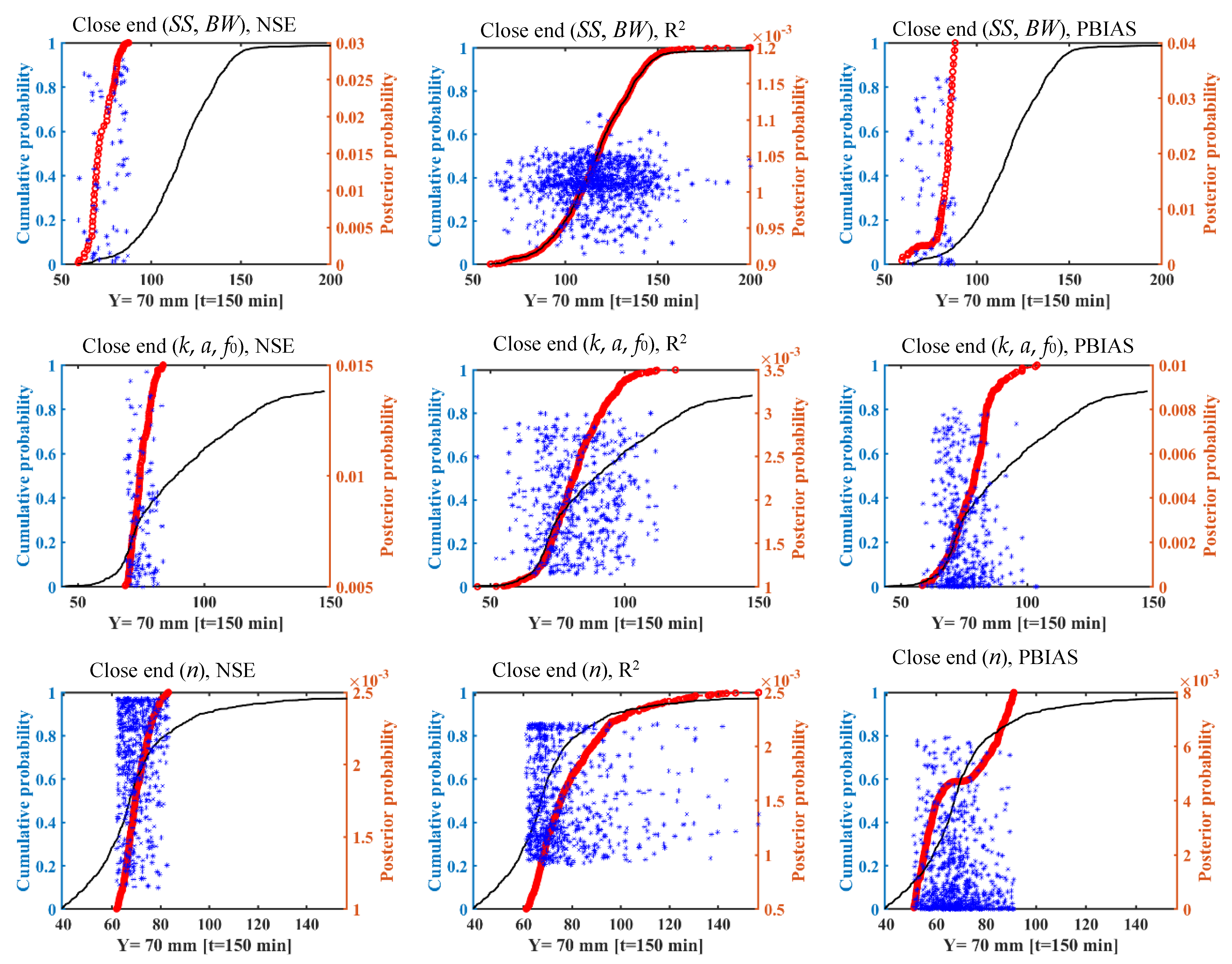
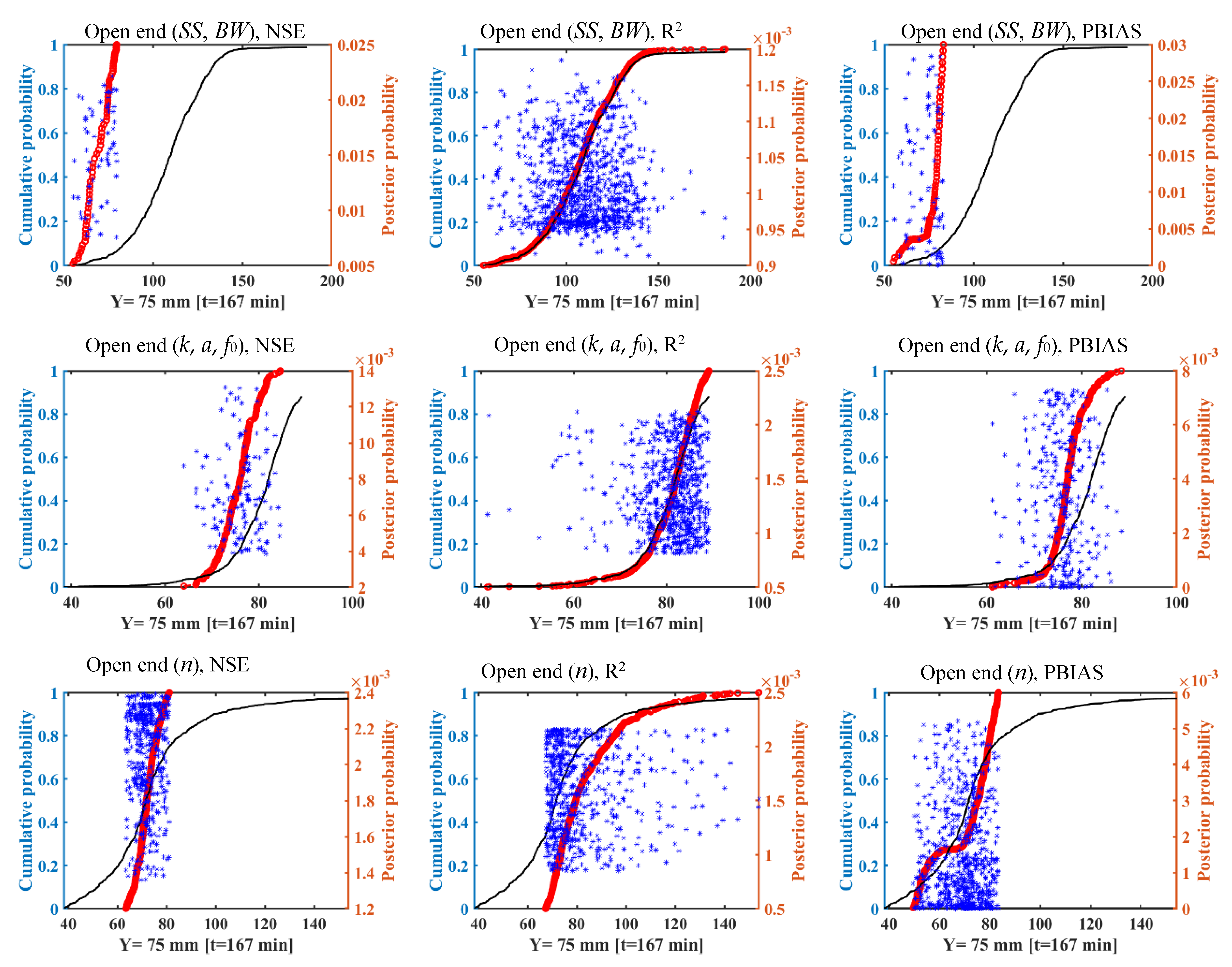
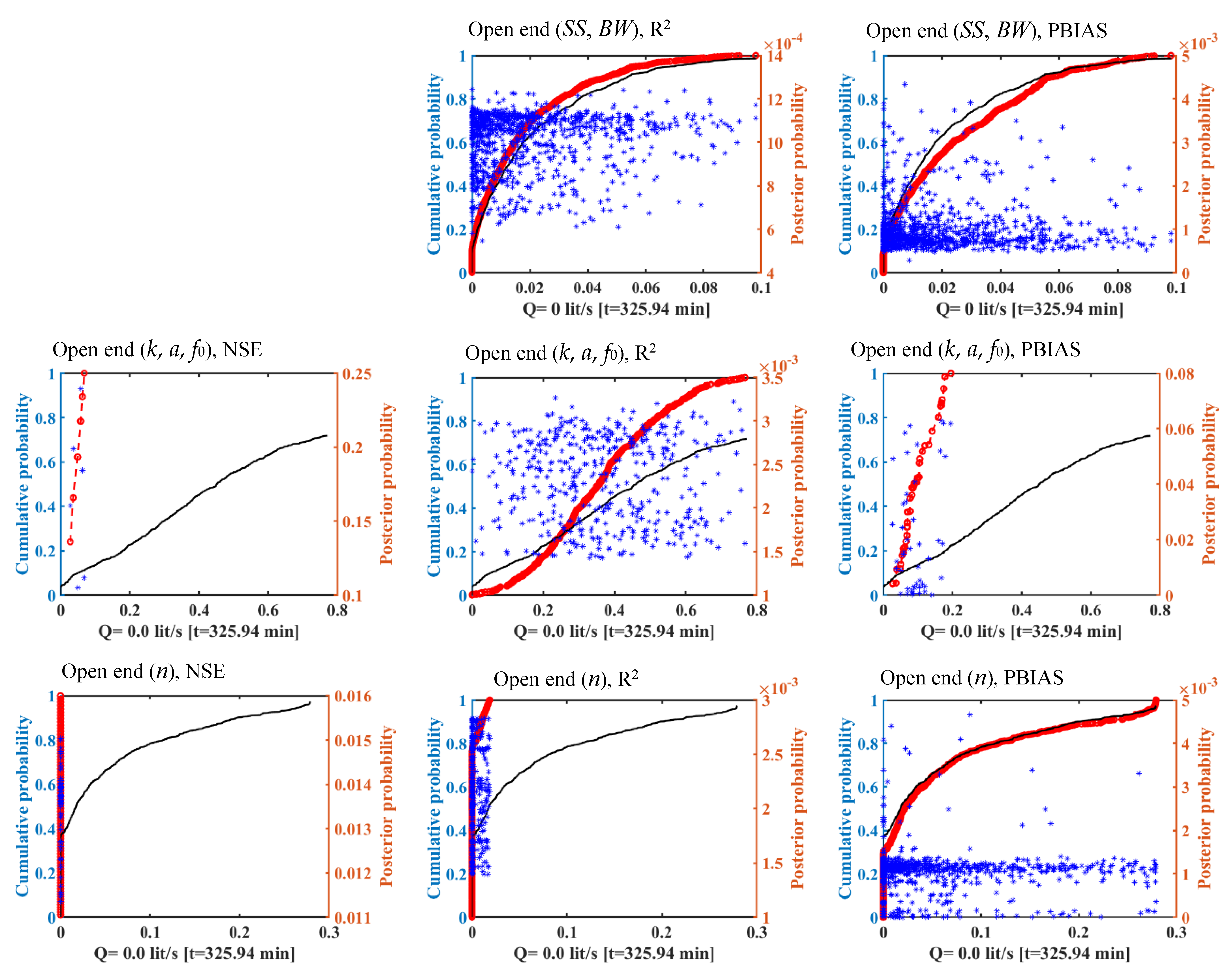
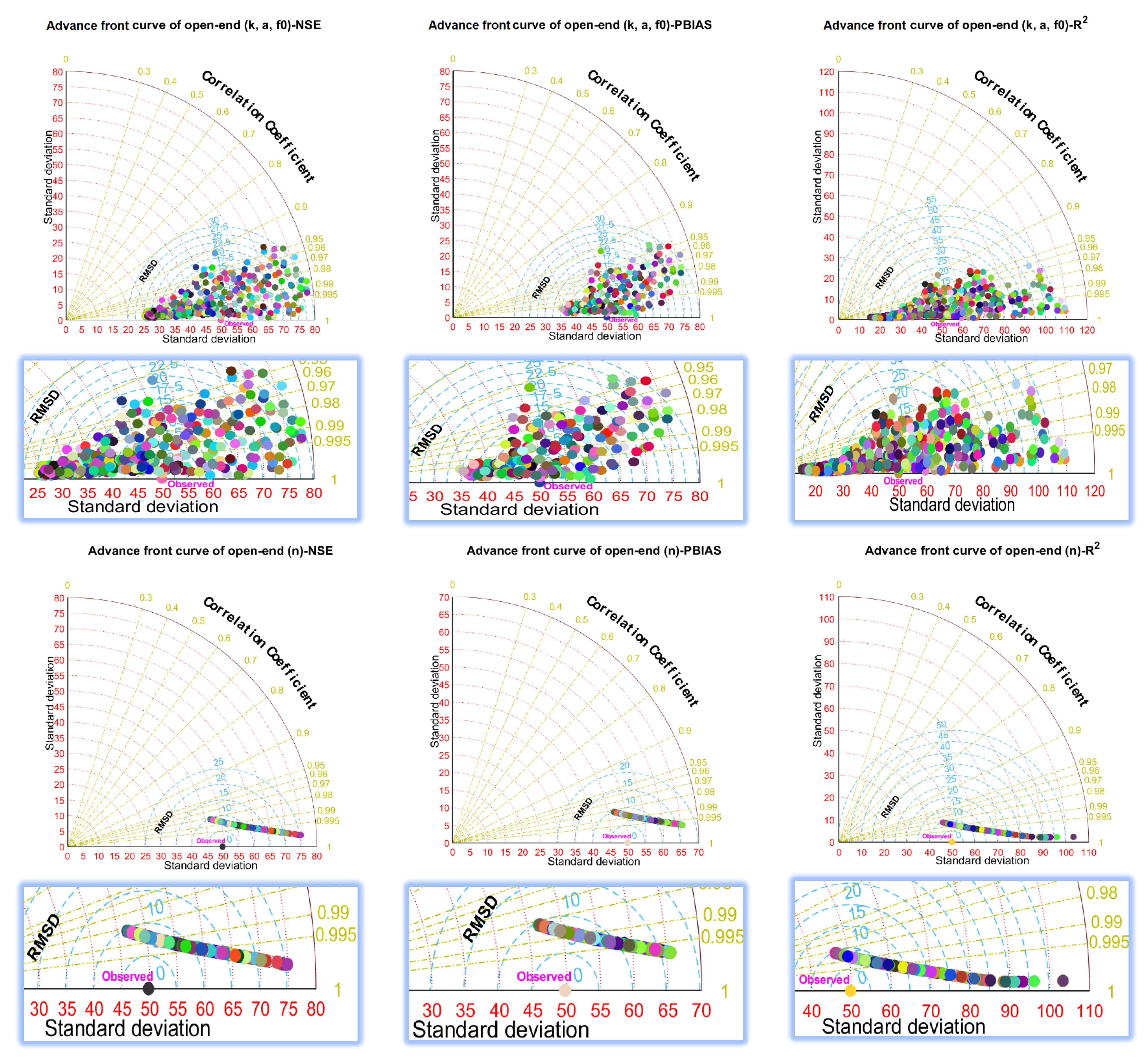
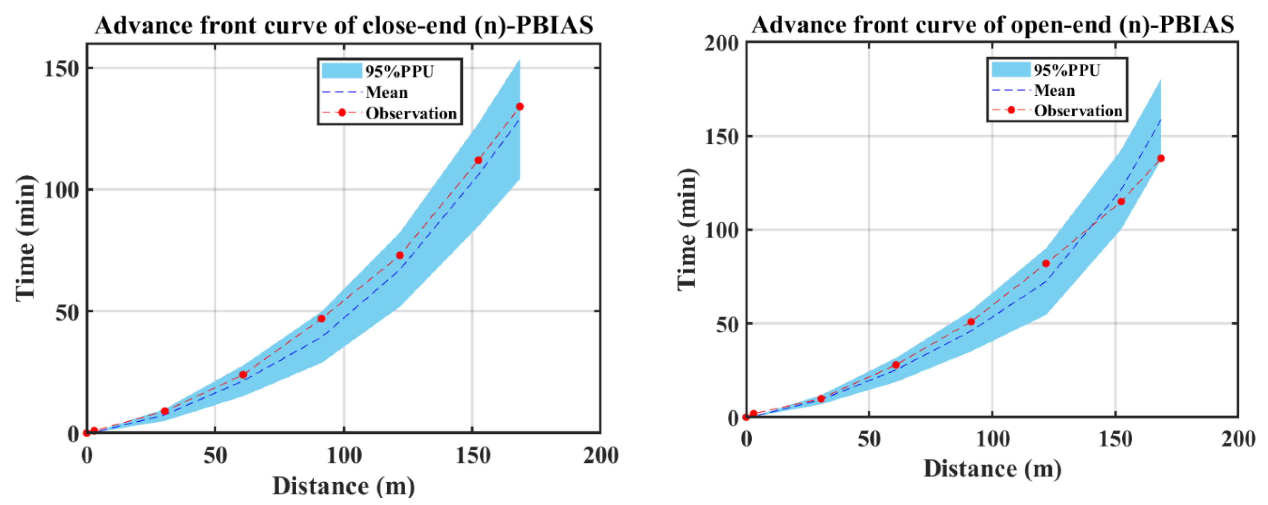
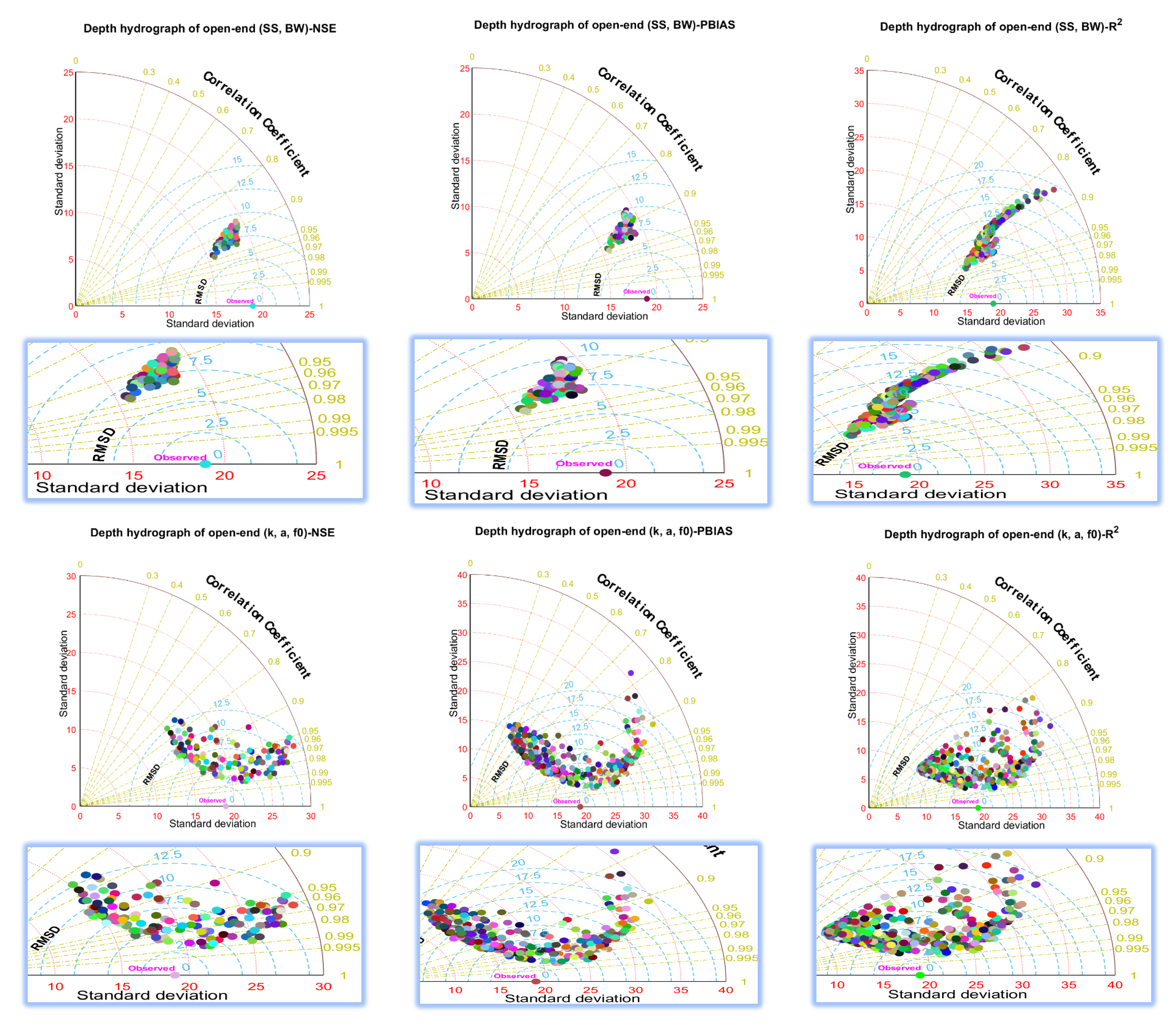
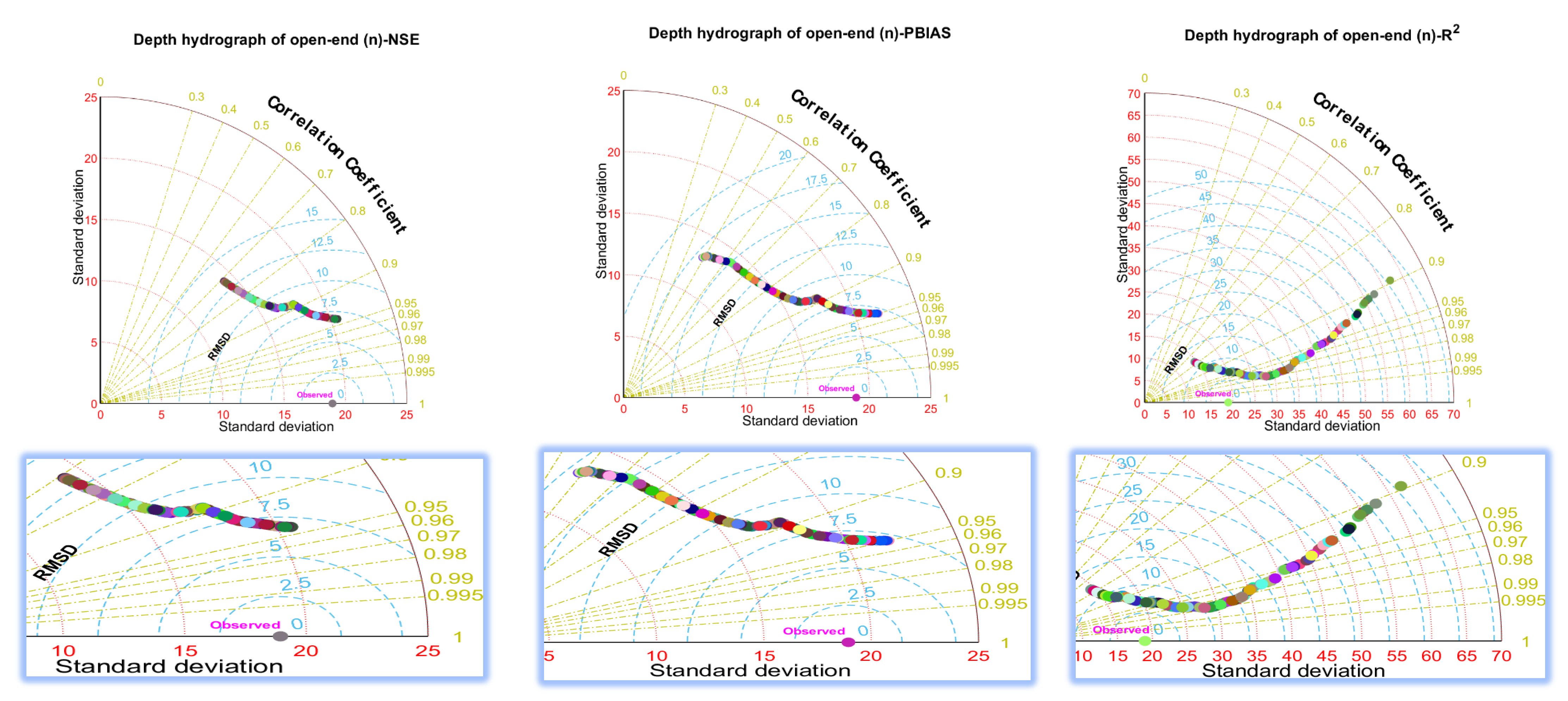
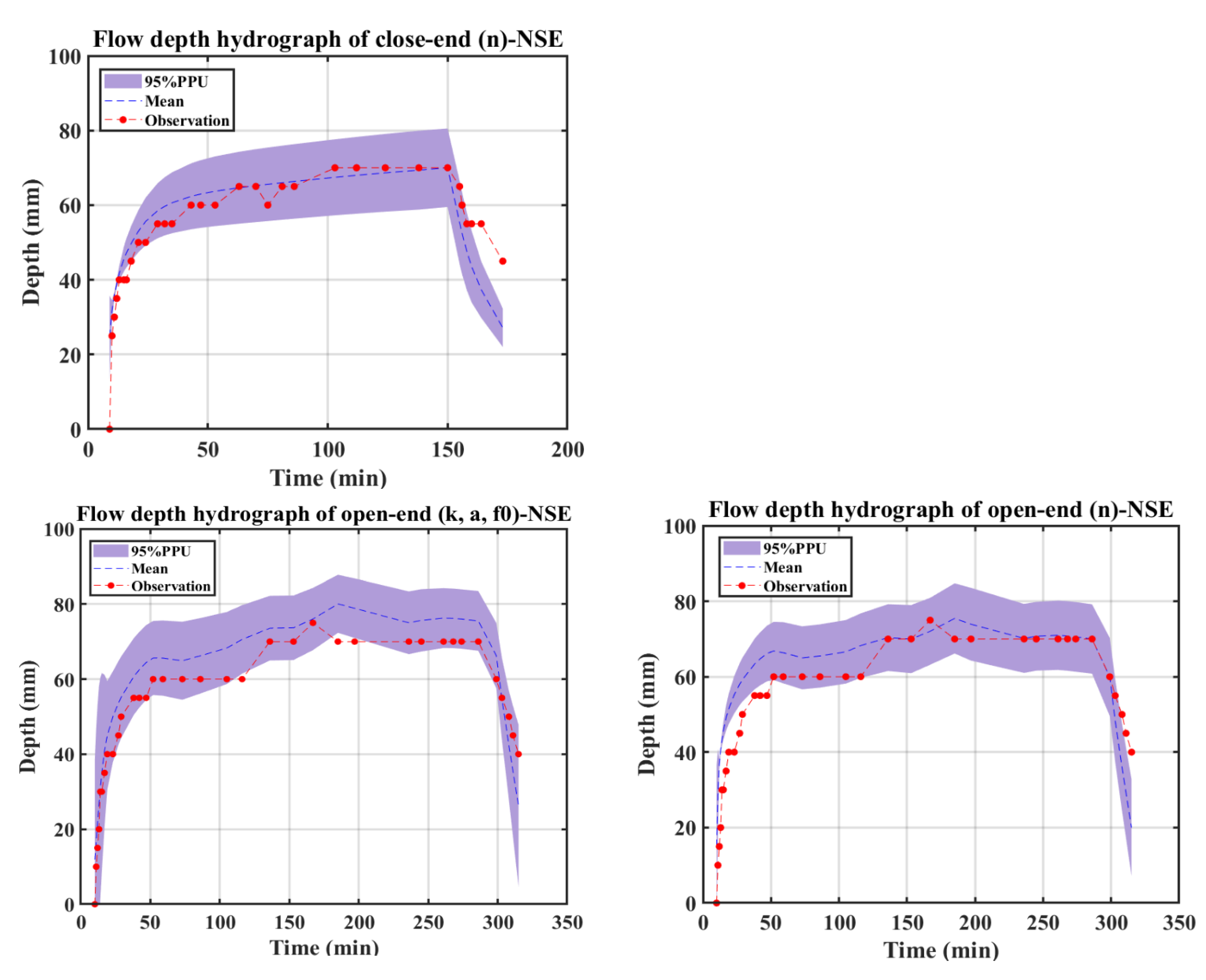
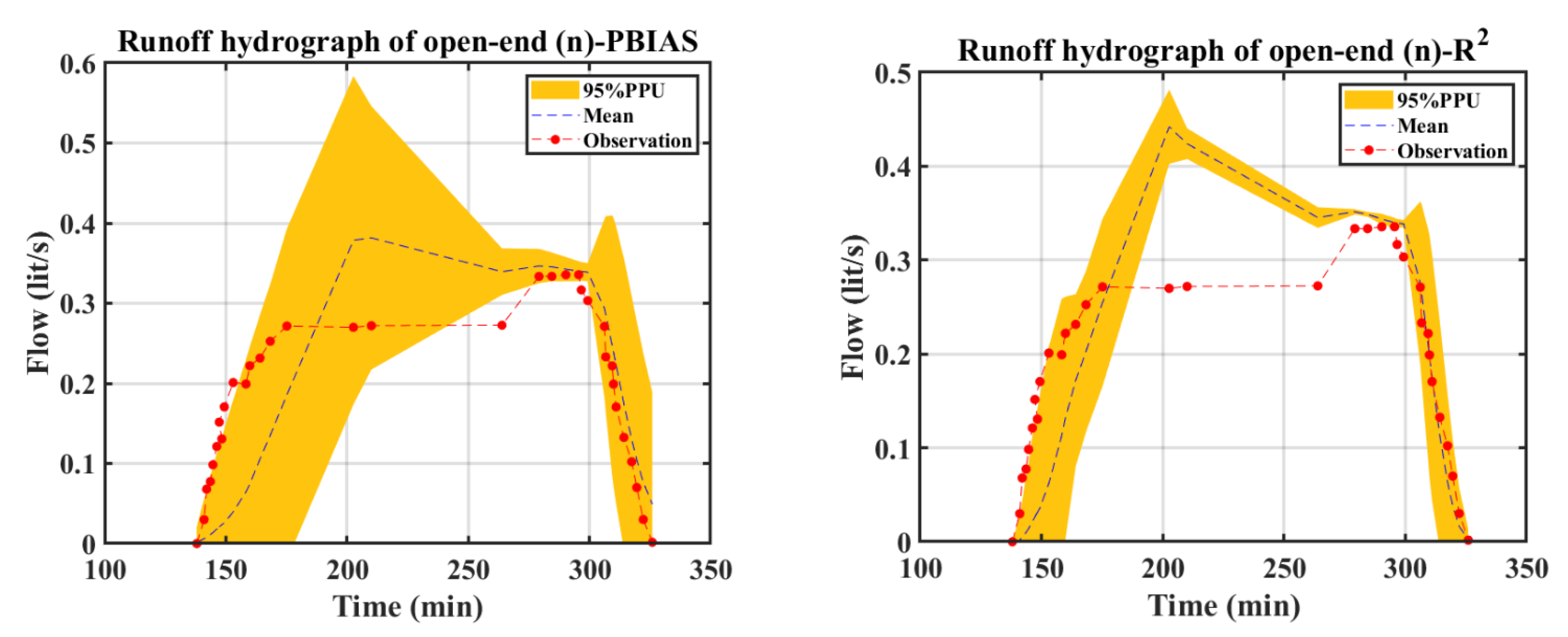
3.2. Simulation Using WinSRFR Furrow Irrigation Model and Uncertainty Analysis

The coefficients information and corresponding probability distributions of Wakeby and Log-Logistic formulations in Table 2 were used to produce random values for each parameter. The created datasets were used as inputs for running the WinSRFR furrow irrigation model in a step-by-step simulation process to solve numerical equations, and then obtain equivalent outputs. This operation was repeated 1000 times by applying the geometry cross section, Kostiakov–Lewis infiltration function, and Manning’s roughness parameters separately until the numerical simulations had completed. Additionally, the simulations were implemented using two conditions of close-ended and open-ended furrow irrigation. Based upon the 2.5% and 97.5% levels of prediction uncertainty, 95% intervals were calculated for the advance front curve, depth hydrograph, and runoff hydrograph, separately. Thus, 95PPU was used to determine the percentage of values bracketed by 95 percent prediction uncertainty. In Figure 1, Figure 2 and Figure 3, the uncertainty bounds are drawn using 2.5% and 97.5% levels. In the next step, the initial uncertainty analysis of the WinSRFR furrow irrigation simulations was performed, and p-factor and r-factor criteria were calculated (Table 2). Figure 1 shows the uncertainty results of the advance front curve for two conditions of close-ended and open-ended furrow irrigation. Figure 1 indicates that the WinSRFR model had high uncertainty levels for predicting advance fronts using the furrow geometry cross section in both conditions. The 95PPU bounds of the close-ended (SS, BW) furrow were found to be outside of almost all the observation values. Based on

Table 3. Uncertainty evaluation using p and r criteria before removing non-behavioral data.

Conditions	Uncertainty Criteria	Advance Front	Depth Hydrograph	Flow Hydrograph
Close end (SS, BW)	p-factor	12.50	34.38
	r-factor	0.11	4.40
Open end (SS, BW)	p-factor	50	52.78	14.71
	r-factor	0.11	3.44	0.48
Close end (k, a, f0)	p-factor	100	100
	r-factor	1.14	3.99
Open end (k, a, f0)	p-factor	87.50	100	100
	r-factor	2.07	2.32	11.49
Close end (n)	p-factor	87.50	100
	r-factor	0.64	3.92
Open end (n)	p-factor	87.50	100	97.06
	r-factor	0.75	3.52	2.07

, only 12.5% and 50% of the observation data for the front curve were bracketed by the 95PPU uncertainty bound in close-ended and open-ended conditions, respectively. These results indicate a high level of model uncertainty for predicting the front curve using geometry cross section parameters. This is due to considering only geometry cross section parameters, while other infiltration, roughness, soil hydraulic properties, and initial and boundary conditions are effective for accurately prediction the advance front using practical irrigation models such as WinSRFR.

According to the p-factor values and 95PPU bounds, better advance estimations were obtained by applying infiltration and roughness parameters. As presented, the 95% confidence interval of the close-ended (k, a, f₀), open-ended (k, a, f₀), close-ended (n), and open-ended (n) ones covers 100%, 87.5%, 87.5%, and 87.5% of the front curve observation data, respectively. Among the infiltration and roughness parameters, the finding results related to the r-factor value demonstrate the superiority of the model based on the Manning’s parameter, especially for the close-ended condition. The calculated r-factor values for the close-ended (n) one are 44%, 69%, and 15% lower than the close-ended (k, a, f₀), open-ended (k, a, f₀), and open-ended (n) ones, respectively. Although infiltration and roughness models create more accurate results than geometry cross section parameters do in estimating front curve, their use still has high instability and uncertainty. The WinSRFR irrigation model uses empirical relationships between the Kostiakov–Lewis and Manning’s functions for representing infiltration and flow processes. Even if physical-based infiltration models can be applied, their practical applications remain limited. It is partly due to problems in coupling infiltration calculations to surface flow models and the difficulty in considering soil hydraulic properties, geometric properties, and other effective parameters [51]. Similar to the uncertainty results of the front curve, WinSRFR has high instability and uncertainty when it is used to estimate the flow depth hydrograph based on the geometry cross section properties of the furrow (Figure 2). Although the results of the p-factor show that all the observation flow depth data are covered by the 95PPU bound, the uncertainty bounds are wide, indicating the low accuracy of estimations [52]. However, the estimation ranges of flow depth hydrograph for close-ended (SS, BW) and open-ended (SS, BW) ones were wide. These bounds did not contain the measured values and produced large uncertainties.

When the geometry cross section parameters were used for simulating the runoff hydrograph (Figure 3), the uncertainty bound covered a relatively narrow scope in comparison with that of the Kostiakov–Lewis and Manning’s parameters. In the case of geometry cross section parameters of the furrow irrigation system, the estimation range of WinSRFR did not match that of the observations. For estimation limits of runoff hydrograph using (k, a, f₀) and (n) parameters, most of the observations fell within the confidence intervals of 2.5% and 97.5%. A few observations were higher than those corresponding to the 95PPU limit produced by Manning’s parameter. There is a wide range of estimations in response to the geometry cross section, infiltration, and roughness parameters. This result demonstrates uncertainties in the Kostiakov–Lewis and Manning equations. In addition, the uncertainties may also lead to severe fluctuations in the estimation results, as well as the large variations in the hydrographs patterns in some cases. Therefore, the WinSRFR furrow irrigation model shows some limitations in estimating the advance front curve, flow depth hydrograph, and runoff hydrograph. Cahoon [53] showed that parameters of the Kostiakov–Lewis infiltration function have a strong influence on the advance front curve and flow hydrograph, which is in agreement with the findings of the current study. The results of the current study are in agreement with those stated by Gillies and Smith [54], which reported that soil infiltration parameters of the modified Kostiakov equation are more sensitive to runoff hydrograph than the advance front curve is, indicating the need for the precise measurement of field data. Khoi and Tom [55] presented that the uncertainty of the predicted flow hydrograph using the SWAT model is high, and the model is sensitive to parameters values.

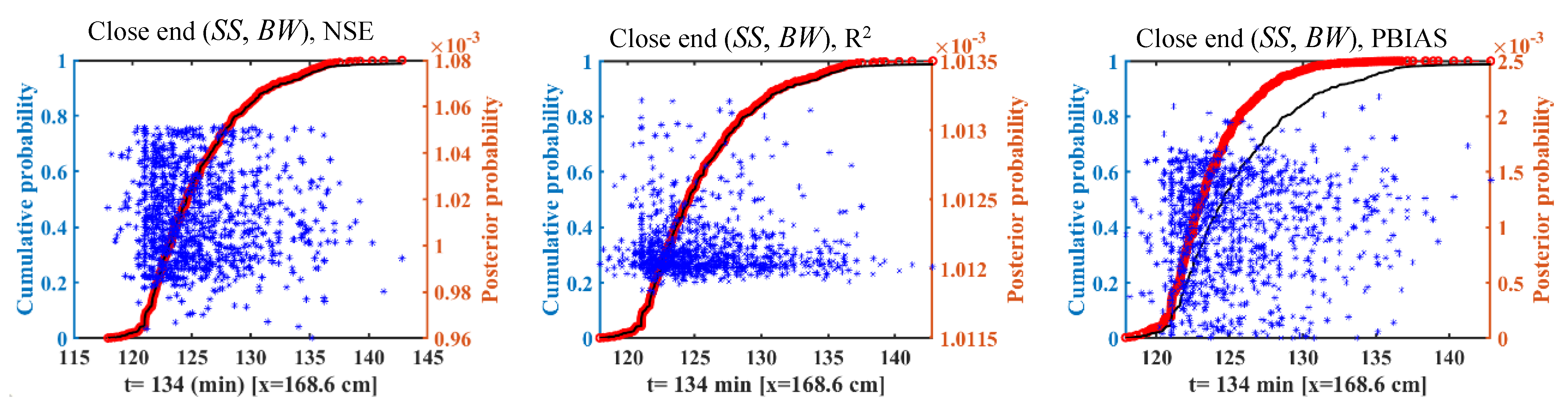
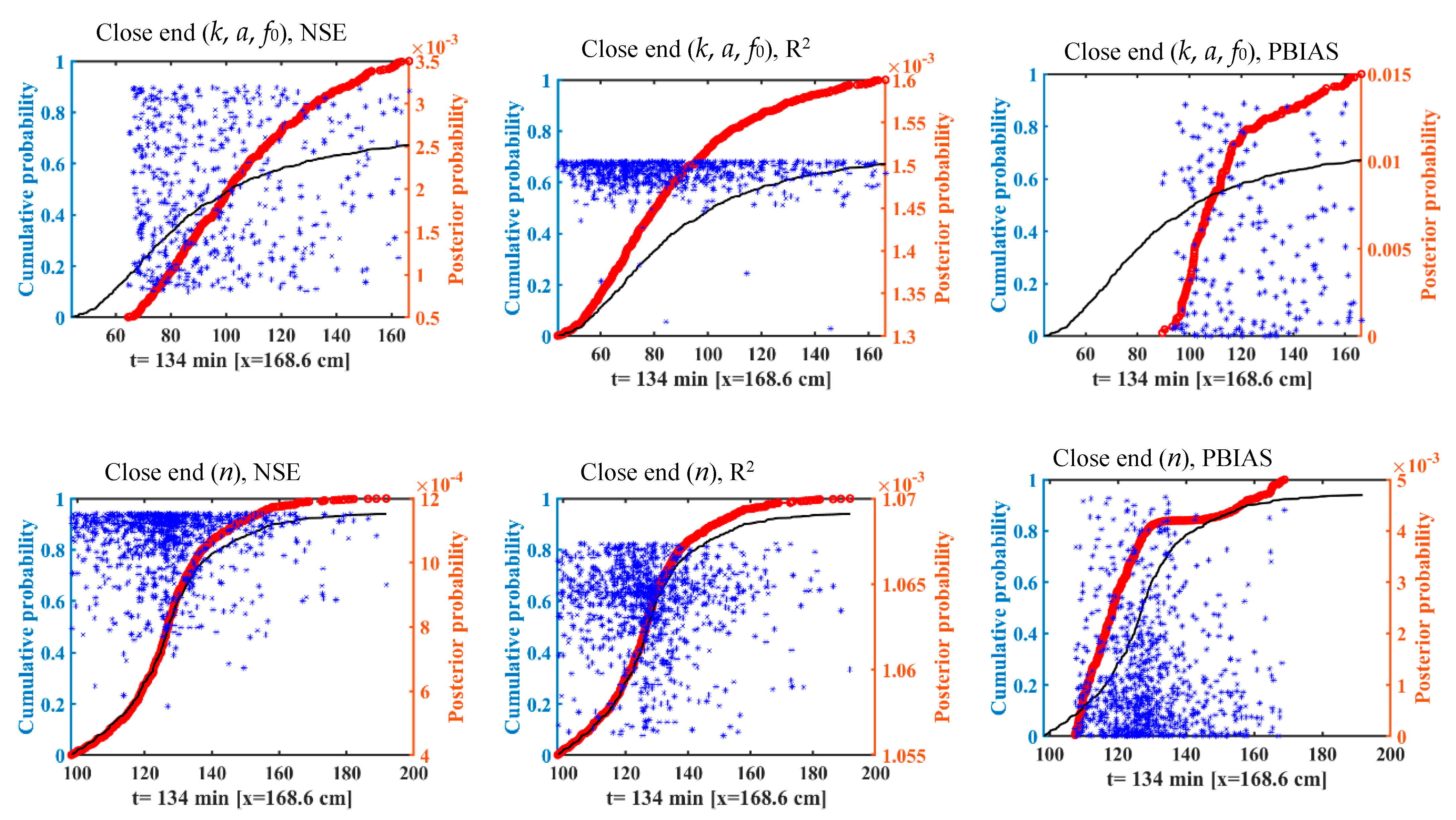
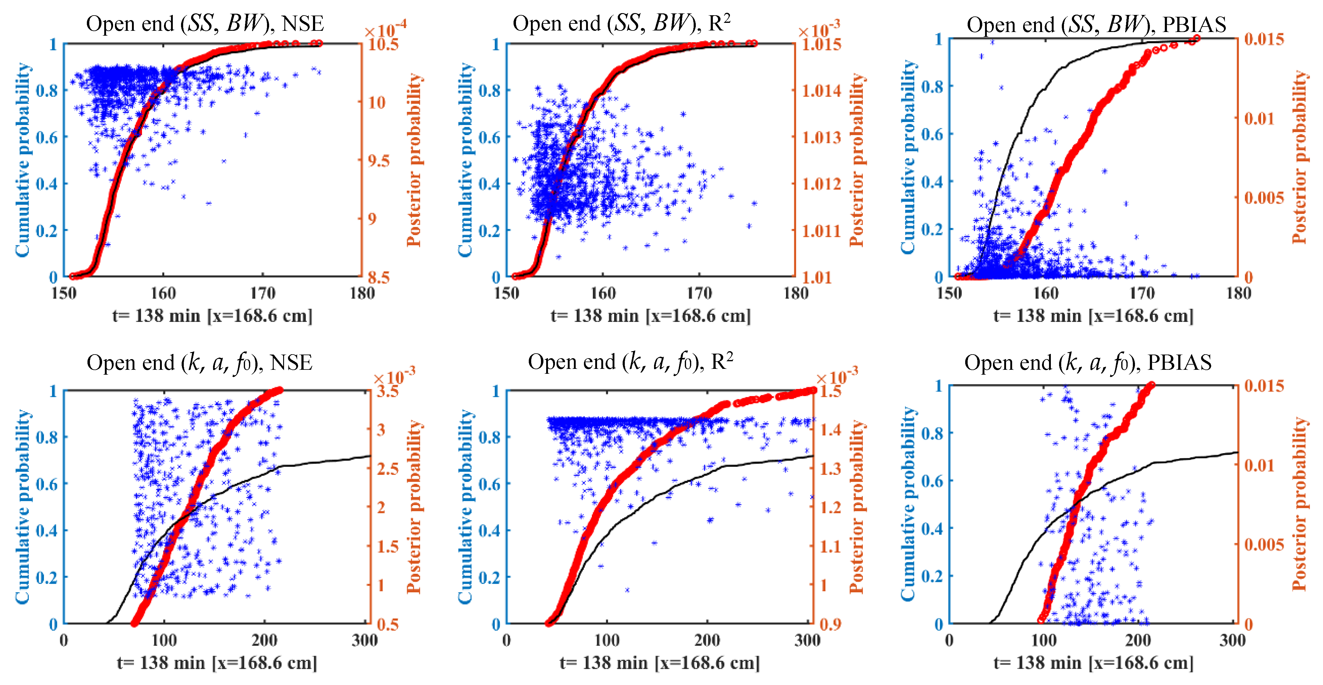
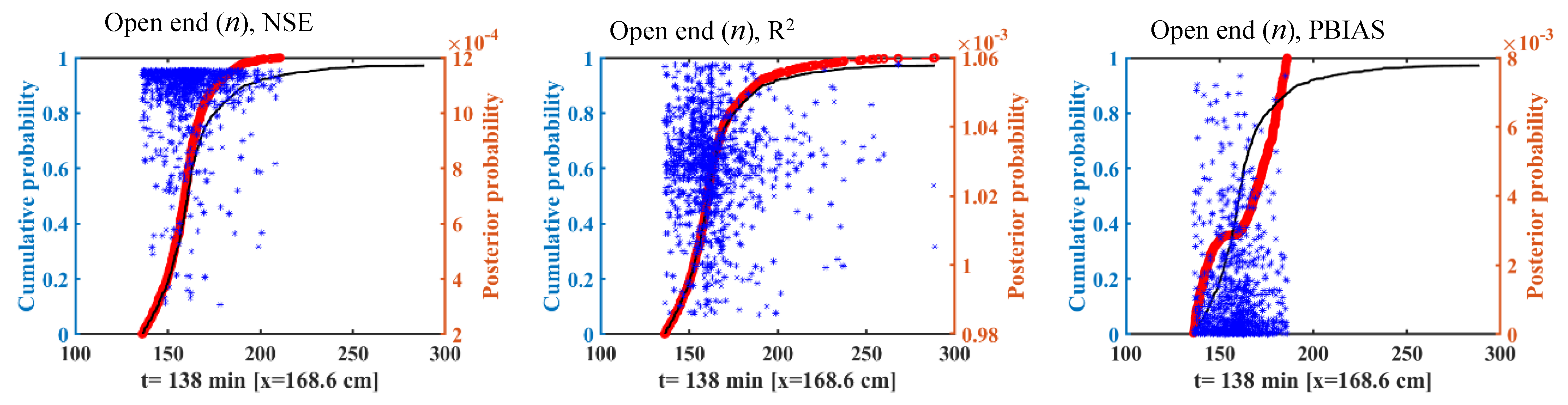
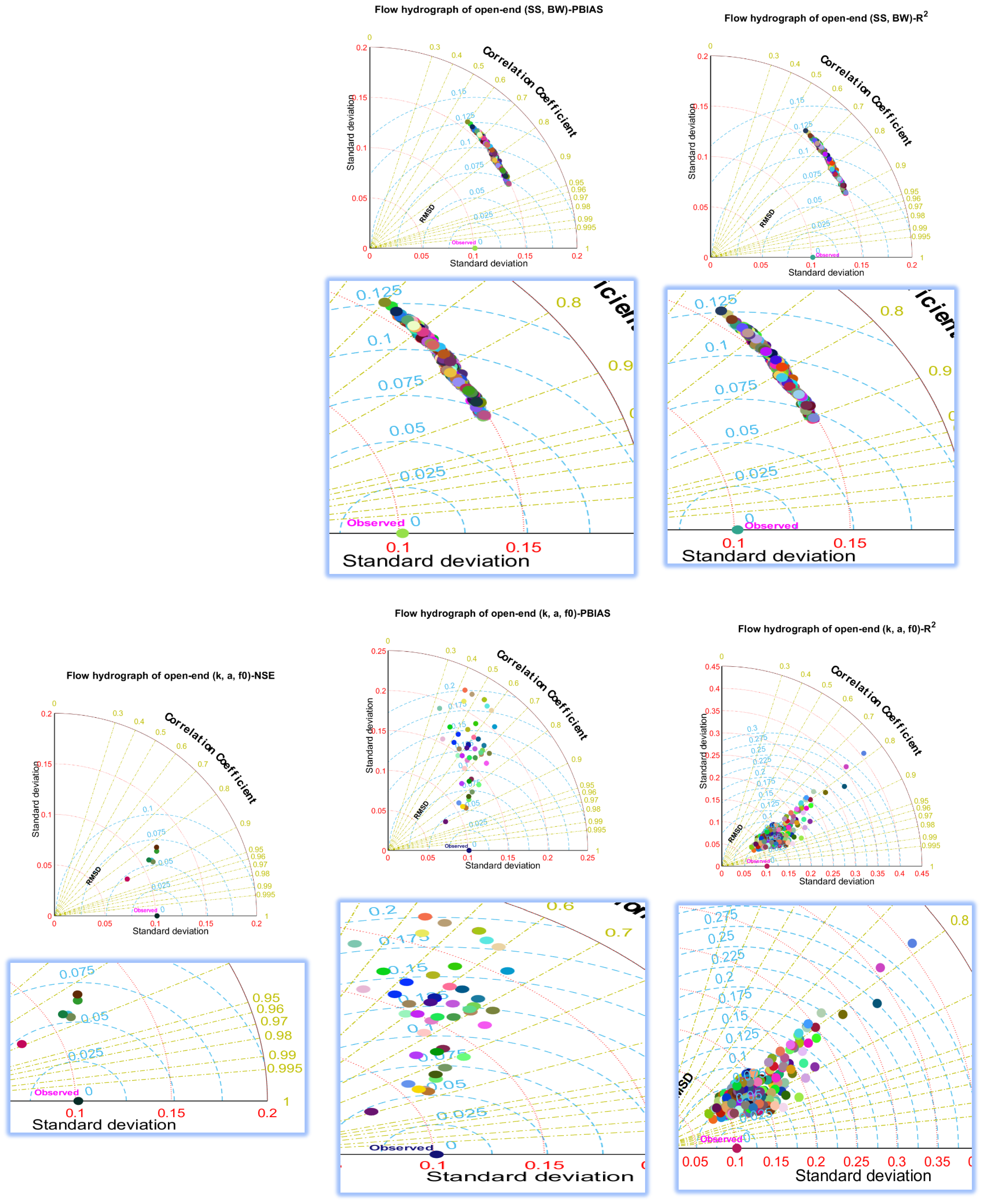
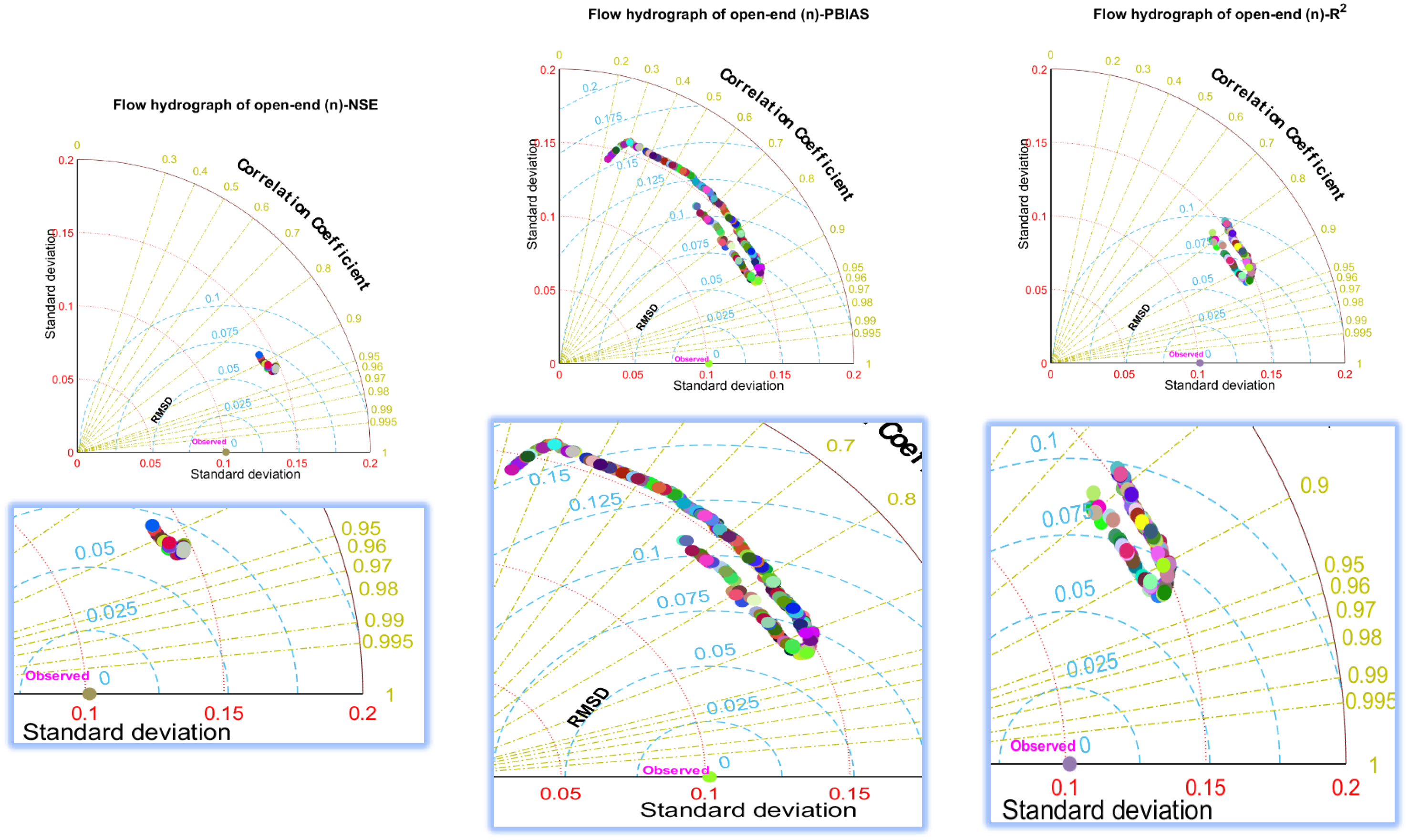
3.3. Effect of Likelihood Measures on Uncertainty

In this section, it is shown how applying likelihood measures affects the uncertainty assessment. Three likelihood measures of NSE, R², and PBIAS are used to investigate their effects on the uncertainty results in WinSRFR furrow irrigation modeling. The percentage of behavioral likelihood, which are derived via GLUE, are given in

Table 4. Percentage of behavioral likelihood derived from the likelihood functions.

Conditions	Likelihood Criteria	Advance Front	Depth Hydrograph	Flow Hydrograph
Close end (SS, BW)	NSE	100	4.76
	R2	100	100
	PBIAS	100	7.69
Open end (SS, BW)	NSE	100	6.58	0
	R2	100	100	100
	PBIAS	100	9.01	100
Close end (k, a, f0)	NSE	56.35	14.06
	R2	76.08	57.37
	PBIAS	21.54	48.75
Open end (k, a, f0)	NSE	53.40	15.76	0.84
	R2	81.41	81.41	59.75
	PBIAS	23.36	35.71	6.41
Close end (n)	NSE	96.61	50.67
	R2	96.61	68.40
	PBIAS	86.64	76.10
Open end (n)	NSE	96.20	50.05	7.61
	R2	100	64.75	47.58
	PBIAS	89.41	72.05	98.56

. Based on the posterior distribution of geometry cross section parameters, 1000 simulations were made by WinSRFR furrow irrigation modeling. All the simulations were behavioral for estimating the front curve based on the geometry cross section properties in both the open-ended and close-ended conditions (NSE > 0.5, −0.25 < PBIAS < 0.25, R² > 0.6). The posterior and prior cumulative distributions of the advance front derived using different criteria for T = 134 min at a distance of 168.6 cm in the close-ended furrow irrigation condition are shown in Figure 4. In simulations of furrow irrigation, the difference between the prior and posterior distributions demonstrated that the model was most sensitive to infiltration parameters for front curves. As seen in Figure 4, the difference is greater for the PBIAS criterion. The dotted points in Figure 4 show the distributions of behavioral data for each parameter, whose likelihood measures NSE > 0.5, −0.25 < PBIAS < 0.25, and R² > 0.6. For the close-ended furrow irrigation condition, the kurtosis in the distribution of the simulation by using roughness parameter and NSE and PBIAS criteria show that this parameter has major effects on advance front curve modeling. Additionally, among the infiltration simulations and dotted plot distribution, the kurtosis of behavioral sets by applying NSE and PBIAS criteria is a more obvious than the other R² is. Hence, it seems the PBIAS and NSE criteria can provide a more efficient way of modeling the front curve based on roughness and infiltration parameters. The acceptable percentages were 96.61% for the close-ended one (n)-NSE; 86.64% for close-ended one (n)-PBIAS; 56.35% for close-ended one (k, a, f₀)-NSE; and 21.54% for close-ended one (k, a, f₀)-PBIAS. Similar results were obtained for the open-ended furrow irrigation condition by applying WinSRFR modeling (Figure 5 and Table 4). Based on Figure 6 and Table 4 and considering the kurtosis of behavioral data, using the roughness parameter and NSE criterion can produce a relatively stable flow depth hydrograph estimation for close-ended furrow irrigation condition. The estimations based on the geometry cross section and infiltration properties by applying the NSE criterion were ranked in second place and can be used after roughness-NSE. Additionally, for the open-ended furrow irrigation condition, the kurtosis distribution of behavioral data displays the role of infiltration (NSE and PBIAS) parameters and geometry cross section (NSE) properties on the estimation stability of WinSRFR (Figure 7). The results of behavioral data dispersion on the posterior distribution line of runoff hydrograph show the effect of the Manning equation on WinSRFR estimation, especially after applying the NSE likelihood function (Figure 8).

It is apparent from the results in Table 4 that many simulations fell within the high likelihood value region (NSE > 0.5). This indicates a complex correlation between the evaluated parameters and the advance front curve output of the WinSRFR model, which can reflect the uncertainty of the model parameters. This result is in agreement with that reported in [9]. Additionally, as seen from Figure 6 to Figure 8, the likelihood measures do not have a regular form for estimating the flow depth and runoff hydrographs. On the other hand, the choices of appropriate likelihood function and simulation criteria are inherently subjective [9]. It is evident that different likelihood functions highlight the role of certain geometry cross section (SS, BW), infiltration (k, a, f₀), and roughness (n) parameters and affect the model’s output uncertainty. Hence, the question is what criterion is useful to investigate the uncertainty of the WinSRFR model for estimating advance front curves and depth and runoff hydrographs. To answer this question, the Taylor diagram and 95PPU bounds were drawn after applying likelihood functions for removing non-behavioral data. The percentage of covered observation, the width of uncertainty bounds, and statistical characteristics were evaluated.

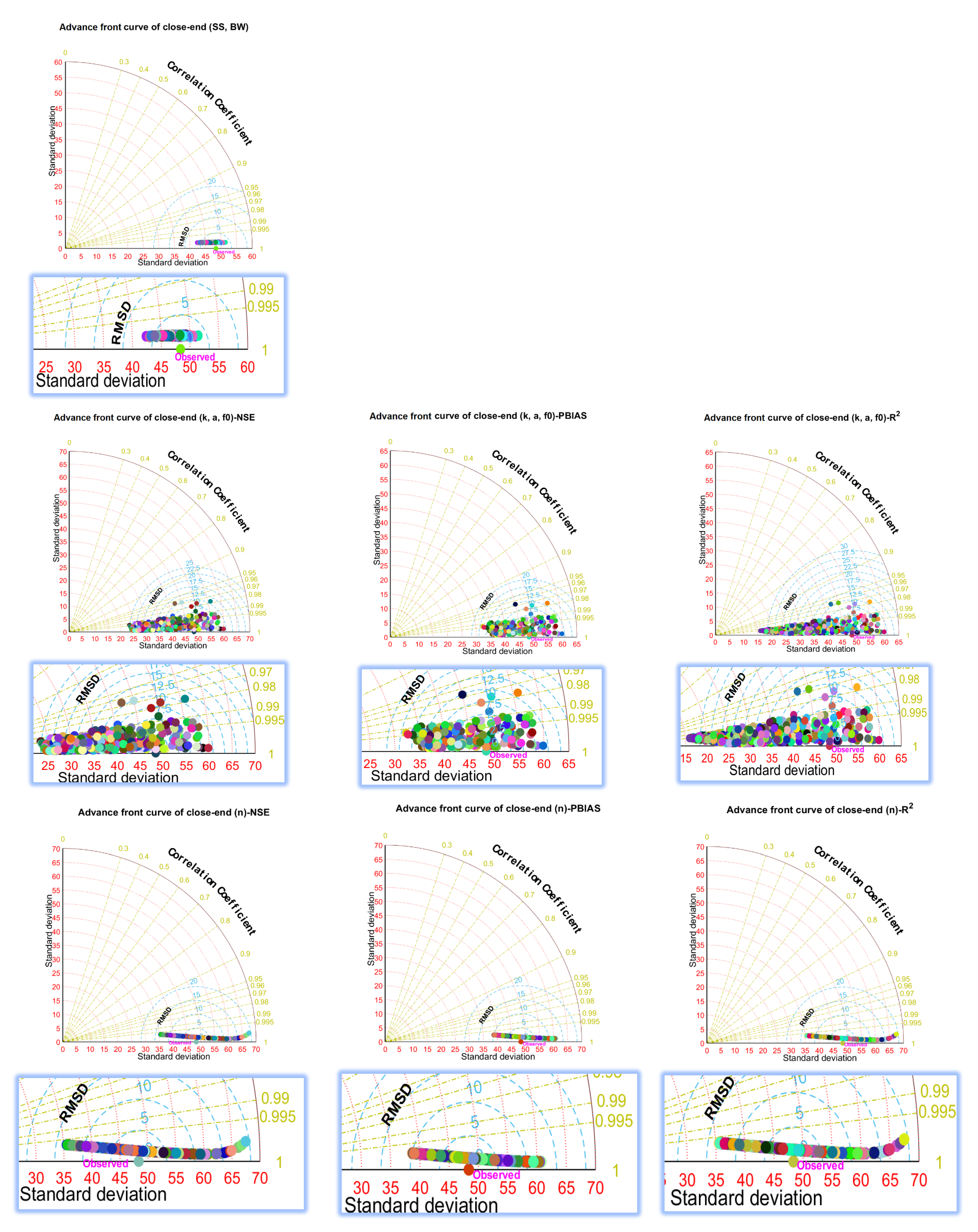
3.4. Analysis of Accuracy and Uncertainty Associated with Different Parameters

In order to achieve precise uncertainty analysis results and a better selection of geometry cross section, infiltration, and roughness parameters, the Taylor diagrams were plotted. This diagram provides a visual of the models’ estimation accuracy based on the three criteria: NSE > 0.5, R² > 0.6, and −0.25 < PBIAS < 0.25. For this aim, those estimations that satisfied the NSE, PBIAS, and R² criteria were selected, and the uncertainty and statistical analyses were performed again.

The results of the Taylor diagram for WinSRFR advance front estimations in the close-ended furrow irrigation condition are shown in Figure 9. Since all the estimations using geometry cross section parameters based on NSE, PBIAS, and R² functions were classified as behavioral data, one Taylor diagram was plotted. The estimations were located between R lines of 0.99 and 1, STD lines of 42.39 and 51.44, and RMSD lines of 1.80 and 6.29 for the advance front curve of close-ended condition (SS, BW). For the estimation of advance front curve using infiltration parameters, the estimations were located between R lines of 0.96 and 1, STD lines of 23.47 and 59.82, and RMSD lines of 0.96 and 25.16 for the NSE function; between R lines of 0.96 and 1, STD lines of 32.49 and 59.82, and RMSD lines of 0.96 and 16.50 for the PBIAS function; between R lines of 0.96 and 1, STD lines of 15.99 and 59.82, and RMSD lines of 0.96 and 32.47 for the R² function. Additionally, for estimation of the advance front curve using the roughness parameter of Manning equation, the estimations were located between R lines of 0.99 and 1, STD lines of 35.56 and 67.52, and RMSD lines of 1.68 and 19.37 for the NSE function; between R lines of 0.99 and 1, STD lines of 38.77 and 60.74, and RMSD lines of 1.68 and 12.44 for the PBIAS function; between R lines of 0.99 and 1, STD lines of 35.56 and 67.52, and RMSD lines of 1.68 and 19.37 for the R² function. It is obvious that all estimations in terms of R exhibit high accuracy in predicting advance front curve in the close-ended condition. Taylor diagrams show that (SS, BW), (k, a, f₀)-PBIAS, and (n)-PBIAS have high accuracy in recognizing the complex relationships between the input parameters and advance front curve. For a better selection of robust parameters, the values of p-factor and r-factor are given in

Table 5. Uncertainty evaluation using p and r criteria after removing non-behavioral data.

Conditions	Criteria	Advance Front			Depth Hydrograph			Flow Hydrograph
		NSE	PBIAS	R2	NSE	PBIAS	R2	NSE	PBIAS	R2
Close end (SS, BW)	p-factor	12.5	12.5	12.5	87.5	90.6	34.38
	r-factor	0.11	0.11	0.11	0.99	1.42	4.40
Open end (SS, BW)	p-factor	50	50	50	77.8	80.56	52.78	0	14.71	14.71
	r-factor	0.11	0.11	0.11	1.05	1.21	3.44	0	0.48	0.48
Close end (k, a, f0)	p-factor	87.5	87.5	87.5	62.5	100	100
	r-factor	0.63	0.51	0.70	1.06	2.09	3.06
Open end (k, a, f0)	p-factor	87.5	87.5	87.5	94.45	100	100	32.37	41.18	44.12
	r-factor	0.88	0.66	1.44	1.32	1.85	2.24	0.47	1.89	8.98
Close end (n)	p-factor	87.5	87.5	87.5	71.87	90.63	90.63
	r-factor	0.51	0.40	0.51	0.93	1.75	3.10
Open end (n)	p-factor	87.5	87.5	87.5	52.78	72.22	61.11	29.41	91.18	70.59
	r-factor	0.52	0.39	0.75	0.76	1.37	2.69	0.37	2.01	1.06

. The results show that (k, a, f₀)-PBIAS and (n)-PBIAS can cover 87.5% and 87.5% of the observation data, and the widths of the uncertainty bound are 0.51 and 0.40, respectively. By removing non-behavioral data (PBIAS > 0.25 and PBIAS < −0.25), the estimations of (n)-PBIAS reduced the r-factor value from 0.64 to 0.4, while the p-factor was constant (87.5%). The results suggest that if proper soil infiltration parameters are selected and accurate measurements are taken, it is possible to reduce the simulation uncertainty of advance front curves. Therefore, to minimize the simulations uncertainty of the WinSRFR furrow irrigation model, it is important to select appropriate parameters prior to modeling advance front curves. Nie et al. [56] demonstrated that the sensitivity of the advance front curve in the WinSRFR model to soil infiltration parameters is very high. They presented that those simulations results were strongly affected when these parameters were changed. Khorami and Ghahraman [57] solved the Richard equation numerically to simulate soil moisture distribution and soil water infiltration. They reported that the model’s simulation uncertainties are relatively high in terms of moisture and infiltration parameters.

Similar results were obtained for estimating the advance front curve in the open-ended condition. Based on Taylor diagrams (Figure 10), the simulations were grouped into 0.99 and 1 R lines, 53.41 and 61.41 STD lines, 6.85 and 12.87 RMSD lines for (SS, BW); into 0.91 and 1 R lines, 25.22 and 78.29 STD lines, and 1.17 and 31.28 RMSD lines for (k, a, f₀)-NSE; into 0.91 and 1 R lines, 34.90 and 76.30 STD lines, and 1.17 and 31.28 RMSD lines for (k, a, f₀)-PBIAS; into 0.91 and 1 R lines, 15.19 and 109.54 STD lines, and 1.17 and 59.85 RMSD lines for (k, a, f₀)-R²; into 0.98 and 1 R lines, 46.69 and 74.95 STD lines, and 7.65 and 25.38 RMSD lines for (n)-NSE; into 0.98 and 1 R lines, 46.69 and 65.60 STD lines, and 7.65 and 16.46 RMSD lines for (n)-PBIAS; into the 0.98 and 1 R lines, 46.69 and 103.37 STD lines, and 7.65 and 53.65 RMSD lines for (n)-R². It seems that (SS, BW), (k, a, f₀)-NSE and (n)-PBIAS produced more accurate simulations than the others did. However, from Table 5, the estimated advance front curve using geometry cross section properties covers only 50% of observations, while the p-factor is 87.5% for soil infiltration and roughness parameters. The r-factor of estimations after removing non-behavioral data show that the uncertainty width of (k, a, f₀)-NSE and (n)-PBIAS reduced from 2.07 to 0.88 and from 0.75 to 0.39, respectively. These results represent that applying the PBIAS function for the roughness parameter of the Manning equation could efficiently reduce uncertain and unstable estimations of the open-ended advance front curve. These uncertainty results indicate an interaction between the accurate measurement of parameters and the output of the WinSRFR model. Nie et al. [58] represented that the performance of the WinSRFR model to simulate water advance and recession trajectories processes are affected by variations in soil infiltration. Moravejalahkamis [59] reported that using a constant value for Manning’s roughness coefficient, soil infiltration properties, field dimensions, inflow rates, and cut-off times in furrow irrigation systems can led to significant errors in advanced recession trajectories assessment. Additionally, several studies suggested that irrigation performance can be improved by considering the soil spatial–temporal variability in soil infiltration and Manning’s roughness parameters [24,31,60]. This statement is in agreement with the results of the current study for the accurate measurement of soil infiltration and Manning’s roughness parameters to achieve the high performance and low uncertainty of the WinSRFR model for simulating the advance front curve.

Figure 11 shows the uncertainty bounds of advance front curve for close-ended and open-ended furrow irrigation conditions after removing non-behavioral data.

The results of Taylor diagrams for estimation flow depth hydrograph in the close-ended furrow irrigation condition are given in Figure 12. From the results of Figure 12, the estimations related to geometry cross section properties are placed between R lines of 0.89 and 0.93, STD lines of 12.78 and 14.81, and RMSD lines of 5.92 and 6.90 after applying the NSE > 0.5 function. The function of −0.25 < PBIAS < 0.25 resulted in 0.89 < R < 0.93, 12.69 < STD < 12.64, and 5.92 < RMSD < 6.95. Additionally, the eliminating non-behavioral data using R² > 0.6 resulted in 0.89 < R < 0.94, 12.69 < STD < 27.40, and 5.89 < RMSD < 14.09. The simulation of the flow depth hydrograph using infiltration parameters of (k, a, f₀) resulted in 0.76 < R < 0.99, 10.76 < STD < 22.99, and 2.59 < RMSD < 10.50 for the NSE likelihood function; 0.40 < R < 0.99, 8.56 < STD < 32.84, and 2.59 < RMSD < 22.14 for the PBIAS likelihood function; 0.78 < R < 0.99, 8.56 < STD < 35.22, and 2.59 < RMSD < 24.90 for the R² likelihood function. By simulating the flow depth hydrograph using the roughness parameter of Manning equation, the minimum and maximum values of R were calculated to be equal to 0.78 and 0.96 for NSE, 0.7 and 0.97 for PBIAS, and 0.78 and 0.97 for R² likelihood functions, respectively. STD values were changed in the ranges of 10.56–19.10, 7.64–23.37, and 10.35–60.03 for NSE, PBIAS, and R² likelihood functions, respectively. The RMSD values were changed in the ranges of 6.02–9.68, 6.02–11.34, and 6.02–47.49 for NSE, PBIAS, and R² likelihood functions, respectively. Based on statistical characteristics, the simulation of flow depth hydrograph using (SS, BW)-NSE, (k, a, f₀)-NSE, and (n)-NSE in the condition of close-ended furrow irrigation are more accurate than the others are. Consequently, from the results shown in Table 4, among three estimations, (k, a, f₀)-NSE resulted in the lowest value of 95PPU and highest value of r-factor, which are equal to 62.5% and 1.06, respectively. Additionally, based on the results in Table 3, it can be concluded that when measurements are dispersed and involve errors, estimations of the flow depth hydrograph using (n)-NSE may reduce uncertainties. The remained behavioral data using NSE > 0.5 for geometry cross section parameters was 4.76%, which shows the instability of SS and BW data due to the measurement errors.

Taylor diagram and uncertainty bound results obtained for WinSRFR flow depth hydrograph simulations in the open-ended furrow irrigation condition are shown in Figure 13 and Figure 14. The analysis of obtained statistical values demonstrated that (SS, BW)-NSE, (k, a, f₀)-NSE, and (n)-NSE had more accurate simulations. The estimations were grouped into R lines of 0.88 and 0.94, STD lines of 15.60 and 19.34, and RMSD lines of 6.66 and 9.21 for (SS, BW)-NSE; into R lines of 0.74 and 0.99, STD lines of 14.33 and 28.82, and RMSD lines of 3.76 and 13.03 for (k, a, f₀)-NSE; into R lines of 0.71 and 0.94, STD lines of 14.17 and 20.54, and RMSD lines of 6.88 and 13.33 for (n)-NSE. Although the 95PPU of (SS, BW)-NSE was 77.8%, which is more than the value related to (n)-NSE, which is equal to 52.78% (Table 5), from the results of Table 4, only 6.58% of the simulations were recognized as behavioral ones. (k, a, f₀)-NSE resulted in the highest 95PPU value, and 94.45% of the simulated data were bracketed by the 95% estimation uncertainty. In both the open-ended and close-ended conditions, the width of the uncertainty bound reduced significantly (Figure 14, Table 3 and Table 5).

Similar results were obtained for simulating the runoff hydrograph, where (k, a, f₀)-NSE and (n)-NSE showed better performances than the other estimations did. Based on the Taylor diagram given in Figure 15, the statistical results of (k, a, f₀)-NSE were calculated as 0.83 < R < 0.89, 0.08 < STD < 0.12, and 0.05 < RMSD < 0.07. The results of 0.88 < R < 0.92, 0.141 < STD < 0.148, and 0.06 < RMSD < 0.07 were obtained for (n)-NSE. When considering the percentage of remained behavioral data (Table 4), it can be seen more than 92% of data were eliminated due to NSE < 0.6. Therefore, re-evaluating the results shows that (n)-PBIAS and (n)-R² reduced the simulating uncertainty of runoff hydrograph while maintaining the 98.56% and 47.58% of the data, respectively. The statistical results of (n)-PBIAS were exhibited to be 0.23 < R < 0.92, 0.06 < STD < 0.16, and 0.138 < RMSD < 0.158. Those results were calculated as 0.77 < R < 0.92, 0.06 < STD < 0.1, and 0.138 < RMSD < 0.153 for (n)-R². Using (n)-PBIAS, 91.18% of observation fell inside the estimated runoff hydrograph. This percentage reduced to 70.59% when (n)-R² was used. The width of uncertainty bound reduced by applying likelihood criteria of −0.25 < PBIAS < 0.25 and R² > 0.6 (Figure 16). Regarding Figure 16 and Table 5, the majority of runoff hydrograph observations were bracketed in the estimated bound by using the PBAIS function. It seems the PBAIS function is able to represent the changes in runoff over time. Some observation points of runoff were beyond the 95PPU estimated by the R² function. Thus, R² was recognized as a modest likelihood function for the runoff hydrograph.

The uncertainty analysis of the WinSRFR model illustrated that the width of the uncertainty bound is commonly affected by the data availability before and after filtering using likelihood functions. This result is in agreement with those presented in [61]. Therefore, the behavior of a furrow irrigation system cannot be accurately predicted by the WinSRFR model because of deficiencies in assumptions of the model, errors in the observed data, monitoring data, model parameters, and the model’s structure error. Large epistemic uncertainties of the WinSRFR simulations can be reduced by minimizing the systematic errors of furrow irrigation measurements, improving the measurement techniques, using more accurate instruments, reducing the inputs errors of the model, and also, considering the model structural error due to the model’s simplification assumptions [62]. In addition, in several previous studies, the WinSRFR model calibrated simulations obtained using optimum parametric sets. While using the GLUE framework, a range of model inputs are transformed into reliable simulations [63]. Through GLUE, a range of model inputs is obtained by identifying the posterior distribution of parameters, and the estimation uncertainty of model outputs is calculated with corresponding confidence intervals [9]. As a result, more attention should be paid to obtaining precise measurements from field experiments for reducing the model’s uncertainty. The results obtained from this study and proposed framework are highly applicable for updating prior knowledge about the reliability of WinSRFR furrow irrigation model outputs.

4. Conclusions

In this study, geometry cross section (SS, BW), Kostiakov–Lewis infiltration (k, a, f₀), and Manning’s roughness (n) parameters in different conditions of furrow irrigation system (close end and open end) were evaluated to analyze the impacts of them on the WinSRFR model outputs. The GLUE analysis was performed by considering three likelihood functions of NSE > 0.5, −0.25 < PBAIS < 0.25, and R² > 0.6 to assess the uncertainty degree of the model outputs response to the input parameters, including advance front curve, flow depth hydrograph, and runoff hydrograph. The following conclusions were drawn from the results:

-

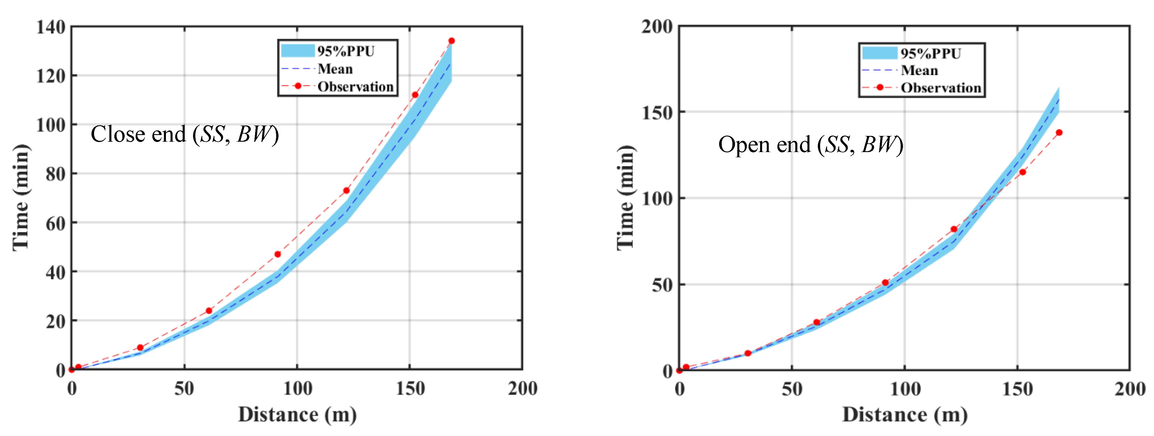
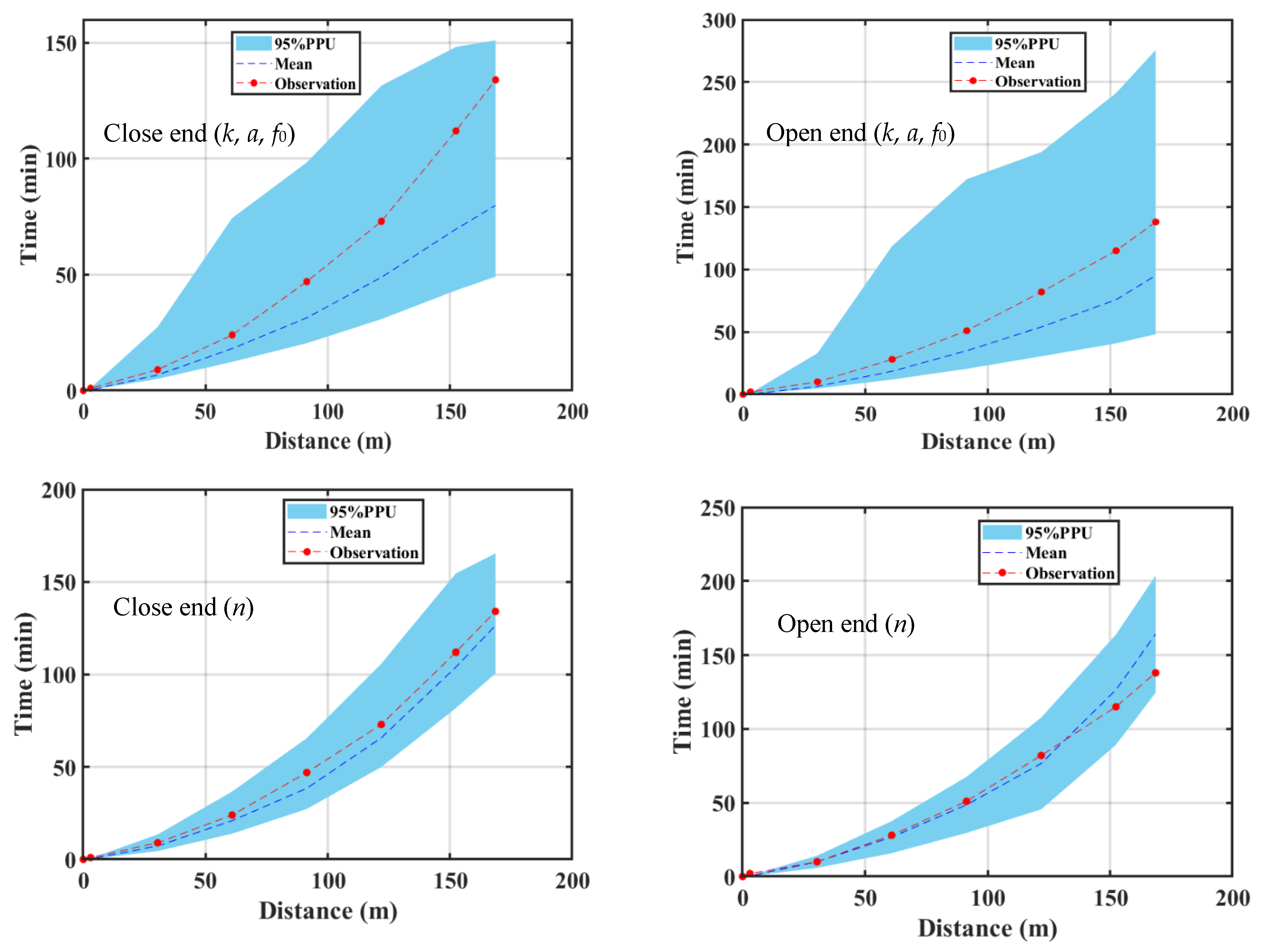
The initial evaluation without filtering non-behavioral estimations showed that the model outputs have high uncertainties in regard to the input parameter of geometry cross section. The value width range of uncertainty bound could be reduced by employing Kostiakov–Lewis infiltration and Manning’s roughness parameters.

-

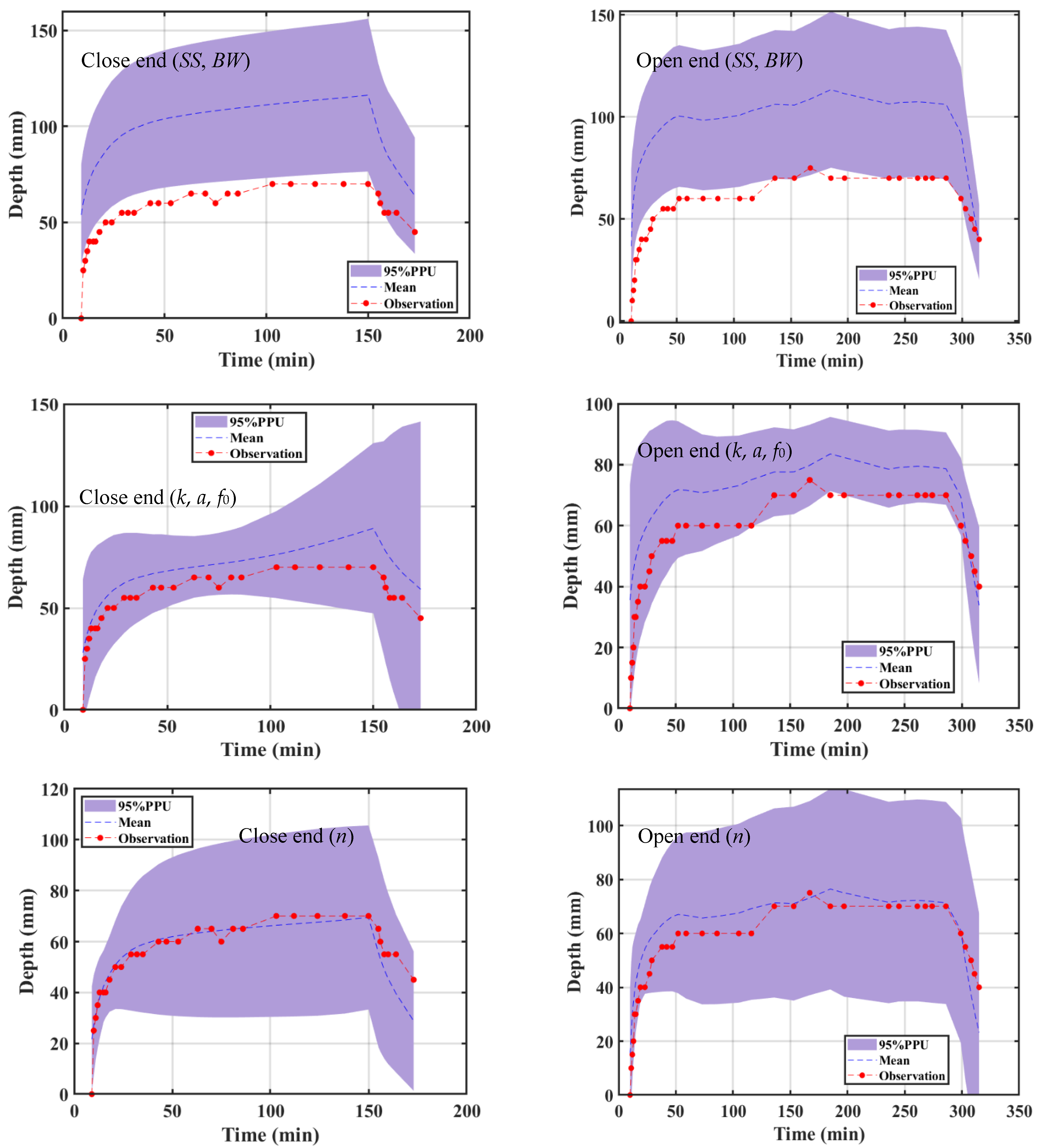
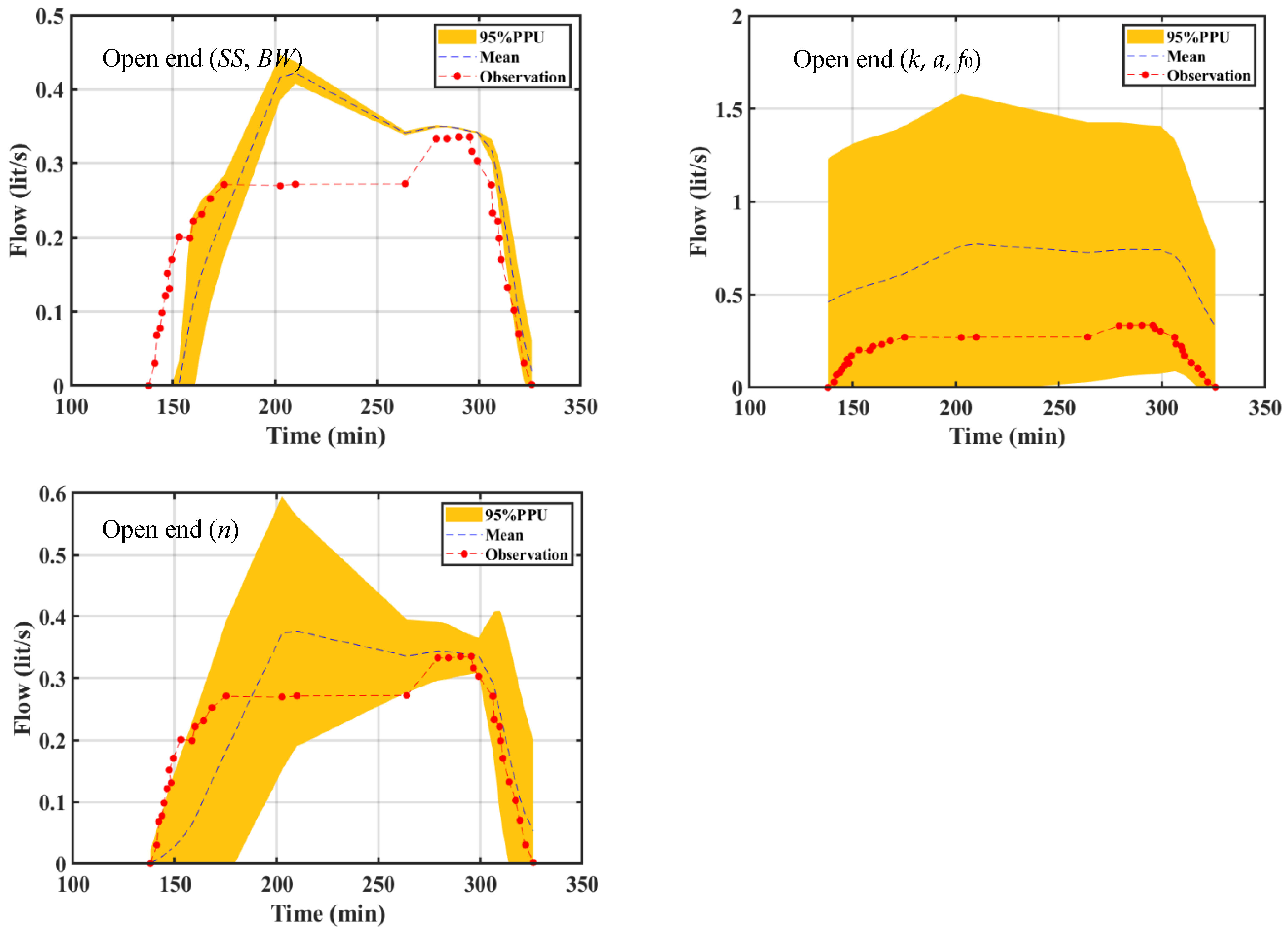
Likelihood measures greatly affect the uncertainty bounds, especially with respect to the Kostiakov–Lewis infiltration and Manning’s roughness parameters. The confidence interval and uncertainty bound of the advance front curve and runoff hydrograph did not change in response to employing likelihood functions for geometry cross section parameters.

-

There is a higher level of instability in the model outputs related to soil infiltration parameters than those related to the roughness coefficient. This result is related to the higher level of sensitivity of the WinSRFR model in inaccurate measurements, methods, and equipment to monitor the soil infiltration than that which is considering for the optimum roughness coefficient.

-

The PBIAS likelihood function played a critical role in the uncertainty results for the estimated advance front curve and runoff hydrograph. In contrast, the NSE likelihood function was more important to implicitly determine the flow depth hydrograph estimation uncertainty. These functions reduced the uncertainty of model outputs by avoiding the parameter sets that produced outputs there were very different from the observations.

According to the current study, it was apparent that likelihood functions affect the model outputs. In addition, this study has limitations, including: (1) considering constant threshold values for likelihood functions of NSE, R², and PBIAS, (2) evaluating limited input parameters, and (3) investigating one source of model uncertainty, which indicate a need for further research. Thus, finding a robust likelihood function with different threshold values is critical because it strongly influences the width of the uncertainty bounds. Additionally, the influence of the length of furrow, inflow, cut-off time, etc., on the model output uncertainty is unknown when one is applying GLUE for WinSRFR-based furrow irrigation applications. Then, future research can consider other epistemic uncertainties such as model structure and more input parameters. This work can also be replicated by implementing different confidence intervals instead of 2.5% and 97.5%. This study provides a conscious understanding of the correlation between the factors affecting furrow irrigation performance. The methodology of this study can be used for complementary studies on the accuracy evaluation of different models of furrow irrigation system simulation. Then, engineers can make more realistic decisions under uncertainty based on the confidence interval bound, which can help to avoid decisions based on incomplete value of models’ prediction.

References

1. Dorigo, W.; Wagner, W.; Albergel, C.; Albrecht, F.; Balsamo, G.; Brocca, L.; Chung, D.; Ertl, M.; Forkel, M.; Gruber, A.; et al. ESA CCI Soil Moisture for improved Earth system understanding: State-of-the art and future directions. Remote Sens. Environ. 2017, 203, 185–215. [Google Scholar] [CrossRef]
2. Nazemi, A.; Wheater, H.S. On inclusion of water resource management in Earth system models—Part 1: Problem definition and representation of water demand. Hydrol. Earth Syst. Sci. 2015, 19, 33–61. [Google Scholar] [CrossRef] [Green Version]
3. Ebrahimian, H.; Liaghat, A. Field evaluation of various mathematical models for furrow and border irrigation systems. Soil Water Res. 2011, 6, 91–101. [Google Scholar] [CrossRef] [Green Version]
4. Mazarei, R.; Mohammadi, A.S.; Ebrahimian, H.; Naseri, A.A. Temporal variability of infiltration and roughness coefficients and furrow irrigation performance under different inflow rates. Agric. Water Manag. 2021, 245, 106465. [Google Scholar] [CrossRef]
5. Koech, R.K.; Smith, R.J.; Gillies, M.H. A real-time optimisation system for automation of furrow irrigation. Irrig. Sci. 2014, 32, 319–327. [Google Scholar] [CrossRef]
6. Brunetti, G.; Šimůnek, J.; Bautista, E. A hybrid finite volume-finite element model for the numerical analysis of furrow irrigation and fertigation. Comput. Electron. Agric. 2018, 150, 312–327. [Google Scholar] [CrossRef] [Green Version]
7. Lalehzari, R.E.Z.A.; Ansari Samani, F.A.R.I.D.E.; Boroomand-nasab, S.A.E.E.D. Analysis of evaluation indicators for furrow irrigation using opportunity time. Irrig. Drain. 2015, 64, 85–92. [Google Scholar] [CrossRef]
8. Bautista, E.; Clemmens, A.J.; Strelkoff, T.S.; Schlegel, J. Modern analysis of surface irrigation systems with WinSRFR. Agric. Water Manag. 2009, 96, 1146–1154. [Google Scholar] [CrossRef]
9. Sun, M.; Zhang, X.; Huo, Z.; Feng, S.; Huang, G.; Mao, X. Uncertainty and sensitivity assessments of an agricultural–hydrological model (RZWQM2) using the GLUE method. J. Hydrol. 2016, 534, 19–30. [Google Scholar] [CrossRef]
10. Beven, K.; Binley, A. The future of distributed models: Model calibration and uncertainty prediction. Hydrol. Process. 1992, 6, 279–298. [Google Scholar] [CrossRef]
11. Mun, S.; Sassenrath, G.F.; Schmidt, A.M.; Lee, N.; Wadsworth, M.C.; Rice, B.; Corbitt, J.Q.; Schneider, J.M.; Tagret, M.L.; Pote, J.; et al. Uncertainty analysis of an irrigation scheduling model for water management in crop production. Agric. Water Manag. 2015, 155, 100–112. [Google Scholar] [CrossRef] [Green Version]
12. Choliz, J.S.; Sarasa, C. Uncertainty in irrigation technology: Insights from a CGE approach. Water 2019, 11, 617. [Google Scholar] [CrossRef] [Green Version]
13. Kisekka, I.; Kandelous, M.M.; Sanden, B.; Hopmans, J.W. Uncertainties in leaching assessment in micro-irrigated fields using water balance approach. Agric. Water Manag. 2019, 213, 107–115. [Google Scholar] [CrossRef] [Green Version]
14. Mondaca-Duarte, F.D.; van Mourik, S.; Balendonck, J.; Voogt, W.; Heinen, M.; van Henten, E.J. Irrigation, crop stress and drainage reduction under uncertainty: A scenario study. Agric. Water Manag. 2020, 230, 105990. [Google Scholar] [CrossRef]
15. Gillies, M.H.; Smith, R.J.; Raine, S.R. Accounting for temporal inflow variation in the inverse solution for infiltration in surface irrigation. Irrig. Sci. 2007, 25, 87–97. [Google Scholar] [CrossRef] [Green Version]
16. Strelkoff, T.S.; Clemmens, A.J.; Bautista, E. Estimation of soil and crop hydraulic properties. J. Irrig. Drain. Eng. 2009, 135, 537–555. [Google Scholar] [CrossRef] [Green Version]
17. Esfandiari, M.; Maheshwari, B.L. Application of the optimization method for estimating infiltration characteristics in furrow irrigation and its comparison with other methods. Agric. Water Manag. 1997, 34, 169–185. [Google Scholar] [CrossRef]
18. Nie, W.; Ma, X.; Fei, L. Evaluation of infiltration models and variability of soil infiltration properties at multiple scales. Irrig. Drain. 2017, 66, 589–599. [Google Scholar] [CrossRef]
19. Kamali, P.; Ebrahimian, H.; Parsinejad, M. Estimation of manning roughness coefficient for vegetated furrows. Irrig. Sci. 2018, 36, 339–348. [Google Scholar] [CrossRef]
20. Oyonarte, N.A.; Mateos, L.; Palomo, M.J. Infiltration variability in furrow irrigation. J. Irrig. Drain. Eng. 2002, 128, 26–33. [Google Scholar] [CrossRef]
21. Bai, M.; Xu, D.; Li, Y.; Pereira, L.S. Stochastic modeling of basins microtopography: Analysis of spatial variability and model testing. Irrig. Sci. 2010, 28, 157–172. [Google Scholar] [CrossRef]
22. Sepaskhah, A.R.; Bondar, H. Sw—Soil and water: Estimation of manning roughness coefficient for bare and vegetated furrow irrigation. Biosyst. Eng. 2002, 82, 351–357. [Google Scholar] [CrossRef]
23. Mailapalli, D.R.; Raghuwanshi, N.S.; Singh, R.; Schmitz, G.H.; Lennartz, F. Spatial and temporal variation of manning’s roughness coefficient in furrow irrigation. J. Irrig. Drain. Eng. 2008, 134, 185–192. [Google Scholar] [CrossRef]
24. Xu, J.; Cai, H.; Saddique, Q.; Wang, X.; Li, L.; Ma, C.; Lu, Y. Evaluation and optimization of border irrigation in different irrigation seasons based on temporal variation of infiltration and roughness. Agric. Water Manag. 2019, 214, 64–77. [Google Scholar] [CrossRef]
25. Walker, W.R.; Skogerboe, G.V. Surface Irrigation: Theory and Practice; Pearson College Div: Logan, UT, USA, 1987; pp. 81–87. [Google Scholar]
26. Clemmens, A.J.; El-Haddad, Z.; Strelkoff, T.S. Assessing the potential for modern surface irrigation in Egypt. Trans. ASAE 1999, 42, 995. [Google Scholar] [CrossRef]
27. Bo, C.; Zhu, O.; Shaohui, Z. Evaluation of hydraulic process and performance of border irrigation with different regular bottom configurations. J. Resour. Ecol. 2012, 3, 151–160. [Google Scholar] [CrossRef]
28. Strelkoff, T.S.; Clemmens, A.J. Approximating wetted perimeter in power-law cross section. J. Irrig. Drain. Eng. 2000, 126, 98–109. [Google Scholar] [CrossRef]
29. Eldeiry, A.A.; Garsia, L.A.; El-Zaher, A.S.A.; El-Sherbini Kiwan, M. Furrow irrigation system design for clay soils in arid regions. Appl. Eng. Agric. 2005, 21, 411–420. [Google Scholar] [CrossRef] [Green Version]
30. Navabian, M.; Liaghat, A.M.; Smith, R.J.; Abbasi, F. Empirical functions for dependent variables in cutback furrow irrigation. Irrig. Sci. 2009, 27, 215–222. [Google Scholar] [CrossRef]
31. Salahou, M.K.; Jiao, X.; Lü, H. Border irrigation performance with distance-based cut-off. Agric. Water Manag. 2018, 201, 27–37. [Google Scholar] [CrossRef]
32. Tung, Y.; Yen, B. Hydrosystem Engineering Uncertainty Analysis; McGraw-Hill Book Company: New York, NY, USA, 2006. [Google Scholar]
33. Setegn, S.G.; Srinivasan, R.; Melesse, A.M.; Dargahi, B. SWAT model application and prediction uncertainty analysis in the Lake Tana Basin, Ethiopia. Hydrol. Process. Int. J. 2010, 24, 357–367. [Google Scholar] [CrossRef]
34. He, J.; Dukes, M.D.; Hochmuth, G.J.; Jones, J.W.; Graham, W.D. Evaluation of sweet corn yield and nitrogen leaching with CERES-Maize considering input parameter uncertainties. Trans. ASABE 2011, 54, 1257–1268. [Google Scholar] [CrossRef]
35. Shafiei, M.; Ghahraman, B.; Saghafian, B.; Davary, K.; Pande, S.; Vazifedoust, M. Uncertainty assessment of the agro-hydrological SWAP model application at field scale: A case study in a dry region. Agric. Water Manag. 2014, 146, 324–334. [Google Scholar] [CrossRef]
36. Tan, J.; Cao, J.; Cui, Y.; Duan, Q.; Gong, W. Comparison of the generalized likelihood uncertainty estimation and Markov Chain Monte Carlo methods for uncertainty analysis of the ORYZA_V3 model. Agron. J. 2019, 111, 555–564. [Google Scholar] [CrossRef]
37. Yan, L.; Jin, J.; Wu, P. Impact of parameter uncertainty and water stress parameterization on wheat growth simulations using CERES-Wheat with GLUE. Agric. Syst. 2020, 181, 102823. [Google Scholar] [CrossRef]
38. Zhang, Y.; Arabi, M.; Paustian, K. Analysis of parameter uncertainty in model simulations of irrigated and rainfed agroecosystems. Environ. Model. Softw. 2020, 126, 104642. [Google Scholar] [CrossRef]
39. Martínez-Ruiz, A.; López-Cruz, I.L.; Ruiz-García, A.; Pineda-Pineda, J.; Sánchez-García, P.; Mendoza-Pérez, C. Uncertainty analysis of the HORTSYST model applied to fertigated tomatoes cultivated in a hydroponic greenhouse system. Span. J. Agric. Res. 2021, 19, e0802. [Google Scholar] [CrossRef]
40. Strelkoff, T.S.; Clemmens, A.J. Hydraulics of Surface Systems Design Operation of Farm Irrigation Systems; Hoffman, G., Evans, R.G., Eds.; American Society of Agricultural and Biological Engineers: St. Joseph, MI, USA, 2007. [Google Scholar]
41. Bautista, E.; Clemmens, A.J.; Strelkoff, T.S.; Niblack, M. Analysis of surface irrigation systems with WinSRFR-Example application. Agric. Water Manag. 2009, 96, 1162–1169. [Google Scholar] [CrossRef]
42. Gillies, M.H. Managing the Effect of Infiltration Variability on Surface Irrigation. Ph.D. Thesis, University of Southern Queensland, Toowoomba, Australia, 2008. [Google Scholar]
43. Bautista, E.; Schlegel, J.L.; Strelkoff, T.S. WinSRFR 4.1-User Manual; USDA-ARS Arid Land Agricultural Research Center: Maricopa, AZ, USA, 2012. [Google Scholar]
44. Seifi, A.; Ehteram, M.; Nayebloei, F.; Soroush, F.; Gharabaghi, B.; Torabi Haghighi, A. GLUE uncertainty analysis of hybrid models for predicting hourly soil temperature and application wavelet coherence analysis for correlation with meteorological variables. Soft Comput. 2021, 25, 10723–10748. [Google Scholar] [CrossRef]
45. Ahmadisharaf, E.; Benham, B.L. Risk-based decision making to evaluate pollutant reduction scenarios. Sci. Total Environ. 2020, 702, 135022. [Google Scholar] [CrossRef]
46. Perea, H. Development, Verification, and Evaluation of a Solute Transport Model in Surface Irrigation. Ph.D. Dissertation, Department of Agricultural and Biosystems Engineering, University of Arizona, Tucson, AZ, USA, 2005. [Google Scholar]
47. Seifi, A.; Ehteram, M.; Soroush, F. Uncertainties of instantaneous influent flow predictions by intelligence models hybridized with multi-objective shark smell optimization algorithm. J. Hydrol. 2020, 587, 124977. [Google Scholar] [CrossRef]
48. Taylor, K.E. Summarizing multiple aspects of model performance in a single diagram. J. Geophys. Res. Atmos. 2001, 106, 7183–7192. [Google Scholar] [CrossRef]
49. Seifi, A.; Dehghani, M.; Singh, V.P. Uncertainty analysis of water quality index (WQI) for groundwater quality evaluation: Application of Monte-Carlo method for weight allocation. Ecol. Indic. 2020, 117, 106653. [Google Scholar] [CrossRef]
50. Logez, M.; Maire, A.; Argillier, C. Monte-Carlo methods to assess the uncertainty related to the use of predictive multimetric indices. Ecol. Indic. 2019, 96, 52–58. [Google Scholar] [CrossRef]
51. Perea, H.; Bautista, E.; Hunsaker, D.J.; Strelkoff, T.S.; Williams, C.; Adamsen, F.J. Nonuniform and unsteady solute transport in furrow irrigation. II: Description of field experiments and calibration of infiltration and roughness coefficients. J. Irrig. Drain. Eng. 2011, 137, 315–326. [Google Scholar] [CrossRef]
52. Seifi, A.; Ehteram, M.; Dehghani, M. A robust integrated Bayesian multi-model uncertainty estimation framework (IBMUEF) for quantifying the uncertainty of hybrid meta-heuristic in global horizontal irradiation predictions. Energy Convers. Manag. 2021, 241, 114292. [Google Scholar] [CrossRef]
53. Cahoon, J. Kostiakov infiltration parameters from kinematic wave model. J. Irrig. Drain. Eng. 1998, 124, 127–130. [Google Scholar] [CrossRef]
54. Gillies, M.H.; Smith, R.J. Infiltration parameters from surface irrigation advance and run-off data. Irrig. Sci. 2005, 24, 25–35. [Google Scholar] [CrossRef] [Green Version]
55. Khoi, D.N.; Thom, V.T. Parameter uncertainty analysis for simulating streamflow in a river catchment of Vietnam. Glob. Ecol. Conserv. 2015, 4, 538–548. [Google Scholar] [CrossRef] [Green Version]
56. Nie, W.; Fei, L.; Ma, X. Impact of infiltration parameters and Manning roughness on the advance trajectory and irrigation performance for closed-end furrows. Span. J. Agric. Res. 2014, 12, 1180–1191. [Google Scholar] [CrossRef] [Green Version]
57. Khorami, M.; Ghahraman, B. Uncertainty analysis of soil parameters in soil moisture profile uncertainty using fuzzy set theory. Iran-Water Resour. Res. 2017, 13, 126–138. [Google Scholar]
58. Nie, W.B.; Li, Y.B.; Zhang, F.; Ma, X.Y. Optimal discharge for closed-end border irrigation under soil infiltration variability. Agric. Water Manag. 2019, 221, 58–65. [Google Scholar] [CrossRef]
59. Moravejalahkami, B.; Mostafazadeh-Fard, B.; Heidarpour, M.; Abbasi, F. Furrow infiltration and roughness prediction for different furrow inflow hydrographs using a zero-inertia model with a multilevel calibration approach. Biosyst. Eng. 2009, 103, 374–381. [Google Scholar] [CrossRef]
60. Bai, M.; Xu, D.; Li, Y.; Zhang, S.; Liu, S. Coupled impact of spatial variability of infiltration and microtopography on basin irrigation performances. Irrig. Sci. 2017, 35, 437–449. [Google Scholar] [CrossRef]
61. Viola, F.; Noto, L.V.; Cannarozzo, M.; La Loggia, G. Daily streamflow prediction with uncertainty in ephemeral catchments using the GLUE methodology. Phys. Chem. Earth 2009, 34, 701–706. [Google Scholar] [CrossRef]
62. Hantush, M.M.; Zhang, H.X.; Camacho-Rincon, R.A.; Ahmadisharaf, E.; Mohamoud, Y.M. Model Uncertainty Analysis and the Margin of Safety. In Total Maximum Daily Load Development and Implementation: Models, Methods, and Resources; American Society of Civil Engineers: Reston, VA, USA, 2022; pp. 271–306. [Google Scholar]
63. Candela, A.N.G.E.L.A.; Noto, L.V.; Aronica, G. Influence of surface roughness in hydrological response of semiarid catchments. J. Hydrol. 2005, 313, 119–131. [Google Scholar] [CrossRef]
Figure 1. The uncertainty bounds of advance front curve for different furrow irrigation conditions and parameters.
Water 15 01250 g001aWater 15 01250 g001b
Figure 2. The uncertainty bounds of flow depth hydrograph for different furrow irrigation conditions and parameters.
Water 15 01250 g002
Figure 3. The uncertainty bounds of runoff hydrograph for open-ended furrow irrigation conditions and different parameters.
Water 15 01250 g003
Figure 4. Posterior (red line) and prior (black line) cumulative distributions of the advance front model from close-ended irrigation conditions.
Water 15 01250 g004aWater 15 01250 g004b
Figure 5. Posterior (red line) and prior (black line) cumulative distributions of the advance front model from open-ended irrigation conditions.
Water 15 01250 g005aWater 15 01250 g005b
Figure 6. Posterior (red line) and prior (black line) cumulative distributions of the flow depth hydrograph model from close-ended irrigation conditions.
Water 15 01250 g006
Figure 7. Posterior (red line) and prior (black line) cumulative distributions of the flow depth hydrograph model from open-ended irrigation conditions.
Water 15 01250 g007
Figure 8. Posterior (red line) and prior (black line) cumulative distributions of the runoff hydrograph model from open-ended irrigation conditions.
Water 15 01250 g008
Figure 9. The Taylor diagrams of WinSRFR advance front outputs for close-ended furrow irrigation condition after removing non-behavioral data.
Water 15 01250 g009
Figure 10. Taylor diagrams of WinSRFR advance front outputs for open-ended condition furrow irrigation after applying behavioral data.
Water 15 01250 g010aWater 15 01250 g010b
Figure 11. The uncertainty bounds of advance front curve for different furrow irrigation conditions after removing non-behavioral data.
Water 15 01250 g011
Figure 12. Taylor diagrams of WinSRFR flow depth hydrograph outputs in the close-ended condition furrow irrigation after applying behavioral data.
Water 15 01250 g012
Figure 13. Taylor diagrams of WinSRFR flow depth hydrograph outputs in the open-ended condition furrow irrigation after applying behavioral data.
Water 15 01250 g013aWater 15 01250 g013b
Figure 14. The uncertainty bounds of flow depth hydrograph for different furrow irrigation conditions after removing non-behavioral data.
Water 15 01250 g014
Figure 15. Taylor diagrams of WinSRFR runoff hydrograph outputs for open-ended condition furrow irrigation after applying behavioral data.
Water 15 01250 g015aWater 15 01250 g015b
Figure 16. The uncertainty bounds of runoff hydrograph for different furrow irrigation conditions after removing non-behavioral data.
Water 15 01250 g016