A Field Experiment for Tracing Lateral Subsurface Flow in a Post-Glacial Hummocky Arable Soil Landscape

Abstract

Lateral subsurface flow (LSF) is a phenomenon that is widely occurring including the hummocky ground moraine landscape. Due to the heterogeneous structure of the subsurface, transport times of pesticides and nutrients from agricultural areas to adjacent water bodies are difficult to assess. Here, LSF at Luvisol and Regosol plots of an experimental field were studied by applying potassium bromide along a 10 m trench below the plow pan in October 2019. The soil solution was collected in suction cups 3 m downslope of the trench and in April 2021, the soil was sampled down to 1 m depth. Almost no bromide was found in the soil solution except for the 160 cm depth of the Regosol plot after a 541 day period. After the same time, bromide was observed in the 90 cm soil depth directly underneath the application trench of the Luvisol plot. A 3D reconstruction of the subsurface horizon boundaries of the Regosol revealed subsurface heterogeneities such as sand lenses that might have been attributed to the heterogeneous subsurface flow pattern.

1. Introduction

Vast areas in the northern hemisphere are covered by hummocky ground moraine landscapes. In North-East Germany alone, 38,000 km² of the land surface is made of ground and terminal moraines, mainly under agricultural use [1]. In those landscapes the phenomenon of lateral subsurface flow (LSF) occurs, describing the lateral redirection of vertically infiltrating water along sloping, impeding layers, such as horizon boundaries or plough layers in the vadose zone [2]. This may lead to an enhanced transport of pesticides and nutrients into streams and kettleholes adjacent to agricultural fields [3,4]. However, the assessment of transport times for these pollutants remains challenging due to the heterogeneous subsurface structure of the unsaturated zone in glacial till soils.

Techniques for detecting LSF include soil-moisture sensor networks [5], non-invasive methods such as electrical resistivity tomography [6], or dye and salt tracing techniques with Brilliant Blue [7], or Bromide [8]. However, studies to temporally quantify LSF are mostly limited to forested landscapes.

In hummocky ground, moraines under agricultural use, LSF was predicted along the Bt-C-horizon interface via a modelling approach [9]. LSF might also explain the deviations in soil water content increase after precipitation found between similar horizons in a field profile and a lysimeter that was extracted at the sloping field profile in a ground moraine [10]. However, it remains unclear what boundary conditions cause LSF in agricultural landscapes in contrast to forested hillslopes. Filipović et al. [9] suggested that initial soil moisture conditions play an important role in the onset of LSF, whereas Hardie et al. [11] indicated that less precipitation might be required to initiate LSF in agricultural soils than in forests.

LSF was also found along the compacted plough layer of a rice field in southeast China by dye tracing experiments [12]. Small-scale heterogeneities such as sand or clay lenses which are common structural features in glacial till soils enhance the occurrence of funnel flow [13]. Here, LSF might also be initiated if local pore water saturation occurs, e.g., caused by preferential flow through macropores similar to earthworm burrows, while the surrounding soil is not saturated. These so-called hydraulic non-equilibrium (HNE) conditions can lead to a local onset of LSF along B-C-horizon boundaries in morainic soils and have been observed for artificial earthworm burrows [14]. However, these studies reveal only limited information about relevant transport times for pesticides or nutrients via lateral flow.

Field tracer studies, where a conservative solute such as salt, is added to the soil water solution, might give insight into travel times and transport pathways for nutrient and pesticide transport in sloping agricultural soils. Hereby, lateral flow between the B-horizon and a till layer [15], along the organic-mineral boundary [16], or along tree roots [17] was identified in forested landscapes. In agricultural soil, Bero et al. [18] applied a potassium bromide solution to observe LSF in loamy sand soil. However, to enhance tracer distribution within the soil the tracer application was followed by 700 mm of non-continuous overhead irrigation. Thus, the travel pathways of solutes within the soil might be analyzed. However, travel times under naturally occurring rainfall cannot be estimated since irrigation patterns differ from those of natural rainfall Also, by applying irrigation water to the plot more water is added than under average precipitation conditions simulating a more humid climate. In most field experiments the tracer is applied as a solution. For example, Gerke and Köhne [19] simulated the previously observed LSF in a tile-drained glacial till field 20 days after irrigating the plots with 98 L of KBr-solution by using a dual-porosity model approach. In a field experiment by Logsdon [20], KBr solution was added by a hand sprayer in a 6 m long trench (1900 kg/ha) at two sites in a glacial till. At the first site, the tracer was recovered 6–15 m downslope from the trench in the capillary fringe over the water table after five months. At the second site, the tracer travelled only 3 m downslope. This difference in travel times was attributed to a deeper groundwater table at the second site.

To analyze solute transport times under natural precipitation conditions in the field it is necessary to conduct experiments without artificial irrigation. For example, Bathke et al. [21] identified LSF in a Bt-horizon over layers with an abrupt change in porosity after 250 days and 450 mm of cumulative rainfall 0.75 to 1.5 m downslope from the bromide application trench. In contrast, Robinson et al. [22] measured a much faster bromide distribution over longer distances in a sandy parent C below an argic horizon. They were able to detect the bromide via electrical resistivity imaging (ERI) after 4 days and 25 mm of cumulative rainfall in depths of 2.5 m and 6 m downslope from the tracer application trench. However, these fast transport times could be explained by the highly conductive sandy material of the C-horizon and the presence of drainage ditches.

In hummocky ground moraines, those studies on actual time scales of lateral water and solute transport under natural precipitation and changing climate conditions in the vadose zone are missing. Filipović et al. [9] numerically predicted LSF along the Btg-C-horizon boundary after high-intensity rainfall within 12 h over distances of approximately 50 cm. However, these simulations have not yet been verified by a field experiment under naturally occurring rainfall. Furthermore, the influence of subsequent dry years on the transport times of LSF is unknown. From 2018 to 2021, consecutive drought events were observed, especially in northeast Germany ([23]; German drought monitor (UFZ): [24]).

Thus, the objectives of this study are (1) to identify LSF in the vadose zone of field soils, (2) to analyse how LSF is related to the subsurface soil structure, and (3) to estimate vertical and lateral subsurface transport pathways. Therefore, a tracer experiment was carried out with potassium bromide application in two different soils (Haplic Regosol and Haplic Luvisol) in a hummocky ground moraine in northeast Germany. The tracer was applied as a solid substance to allow for a defined spatial distribution under naturally occurring rainfall. The temporal dimensions, i.e., travel times; of the tracer movement will be quantified in these heterogeneous soils during subsequent dry years (2019–2021). By visualising the subsurface in 3D-model potential pathways for the subsurface water movement will be identified.

2. Materials and Methods

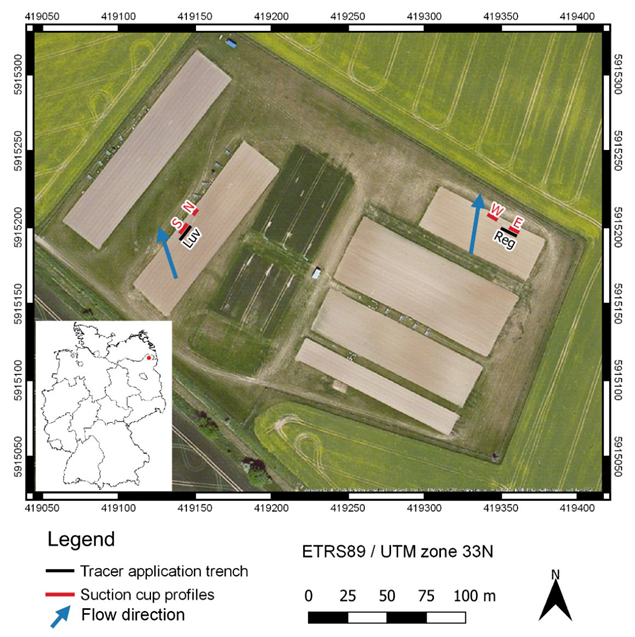
2.1. Study Site

The experiments were carried out in a hummocky arable soil landscape at the “CarboZALF-D” experimental field site [25] of the Leibniz-Centre for Agricultural Landscape Research (ZALF), located near the village of Holzendorf in the north of Brandenburg, Germany (53°23′ N, 13°47′ E, 50–60 m asl, c.f. Figure 1). The annual average air temperature (8.6 °C), mean annual precipitation (495 mm), and mean annual potential evapotranspiration (633 mm) were recorded in the experimental station in Dedelow (53°22′ N, 13°48′ E) maintained by the ZALF (www.zalf.de) in the period from 1992 to 2016.

Precipitation was recorded by 5 rain gauges distributed across the experimental site. The data were aggregated into daily sums and manually corrected for outliers. The arithmetic mean of the corrected data was used for further analysis. For more details about the rain gauges and their location refer to [10]. Between 8 October 2019 and 31 October 2021, a total precipitation of 1038 mm was recorded. The annual precipitation in 2020 was 450 mm, 45 mm less than the mean annual precipitation of 495 mm. 2019 and 2020 were both denoted as drought years [23]. Precipitation maxima are found in summer (Figure 2). The highest daily precipitation rates before the arrival of the tracer were recorded on 9 August 2020 (22 mm/day) and 18 August (20.1 mm/day). Average daily temperatures and potential evapotranspiration were measured by an automated weather station (SYNMET/LOG LAMBRECHT meteo GmbH) in Dedelow. Average daily temperatures were recorded 2 m above ground and varied between −10 °C in February 2021 and 27 °C in August 2020 (Figure 2). Potential evapotranspiration was recorded on a daily basis.

Within the field site, two soil types were chosen where the lateral subsurface flow was expected to occur according to [9,26]: a Haplic Luvisol (Luv) and a Haplic Regosol (Reg). Both consist of soil horizons with relatively high saturated hydraulic conductivity values, K_s, of 309.4 (Luv) and 89.5 cm d⁻¹ (Reg) over horizons with lower K_s-values of 31.5 (Luv) and 7.3 cm d⁻¹ (Reg) (

Table 1. Soil physical and hydraulic parameters of the Luvisol (Luv) and Regosol (Reg) adapted with permission from [27] (2012 Elsevier B.V.): ρ_b–soil bulk density; soil texture classes: sand (2–0.063 mm), silt (0.063–0.002) and clay (<0.002 mm); C_org–organic carbon content; K_S–soil hydraulic conductivity (RETC-fitted with the van Genuchten-Mualem model).

Soil	Horizon	Depth	ρb	Sand	Silt	Clay	Corg	KS
		[cm]	[kg m−3]	[g kg−1]	[g kg−1]	[g kg−1]	[%]	[cm d−1]
Luv	Ap	0–31	1490	619	265	116	0.83	22.3
	Btg	31–70	1680	549	265	185	0.44	309.4
	CBkg	70–105	1790	588	258	154	0.15	31.5
Reg	Ap	0–25	1660	596	283	120	0.47	39.4
	CBkg	26–48	1760	614	267	118	0.10	89.5
	Bgk1	49–85	1900	612	270	118	0.02	7.3
	Bgk2	85–190	1910	610	263	127	0.03	16.8

).

Both soils have a sandy texture and tilled topsoil down to 25 to 31 cm. The Luvisol consists of a clay-enriched Btg-horizon with a truncated clay-depleted A-horizon due to erosion processes at the upper part of a sloped field (Table 1). The C-horizon is made of stony glacial till parent material with carbonates. The Regosol consists of a rather shallow topsoil layer that is located directly above the carbonate parent material. Slope inclinations at the Luvisol and Regosol sites are 6 and 13%, respectively [27].

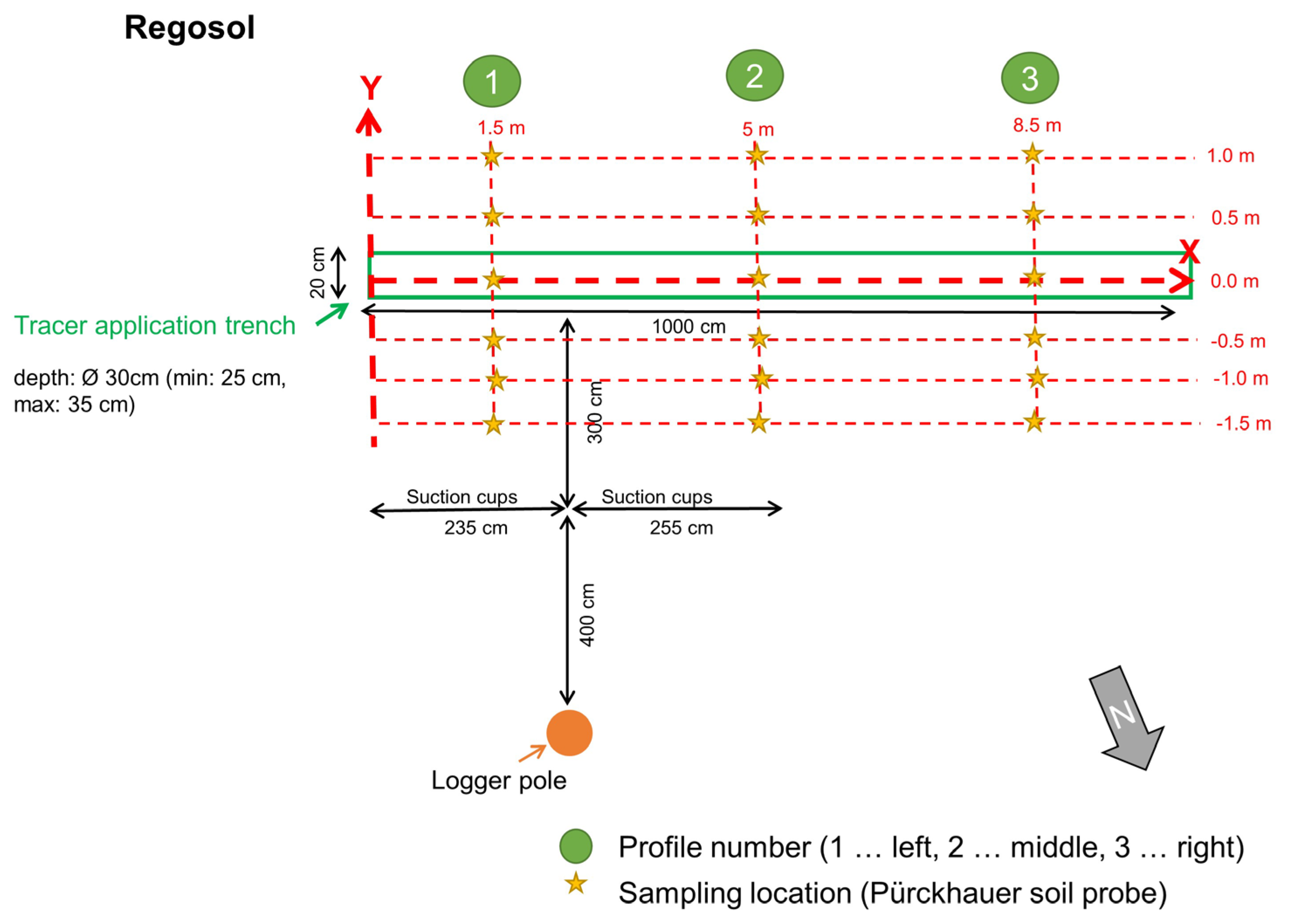
2.2. Bromide Application and Soil Sampling at the Beginning of the Experiment

The Br⁻-Tracer was applied in solid form as KBr powder on 8 and 9 October 2019, one day after tillage by moldboard plowing. The tracer was inserted along a 10 m long and 0.2 m wide trench at 0.25–0.3 m depth just below the consolidated plough pan layer 3 m upslope from the suction cup profiles parallel to the field edge (Figure 1). Each trench was subdivided into 20 sections 0.5 m in length. In each section, the approximately 3 cm thick plough layer was carefully removed and 10 g of KBr (Roth, 99%, p.a.) were distributed uniformly (67 g m⁻² Br⁻). Afterwards, the soil material from the plough layer was backfilled and carefully reconsolidated using a rubber mallet.

Next to the tracer application trench, undisturbed soil cores (100 cm³, height: 5 cm) were collected every 0.5 m to determine the actual soil water content and the bulk density of the plough layer at the application depth. The trench was then refilled with the excavated plowed topsoil. On 14 October 2019, the soil was cultivated with a circular harrow, and winter rye was sown.

The soil samples were weighed at field water content and afterwards, air dried. The dry samples were ground and sieved to analyse the amount of stones (soil particles >2 mm). The mass of the soil fraction <2 mm was again weighed and an aliquot of approx. 15 g of each sample was left to dry at 105 °C for 24 h. Afterwards, the samples were placed in a desiccator during cooling for 0.5 h, weighed, and the dry subsample mass, $M_{d<2}$, was related to the total sample $M_d$ to obtain the gravimetric soil water content, w [g/g] of the fresh samples and the dry bulk density of the total soil, ${\rho }_b=M_d/V_t$. The bulk density related to fine soil <2 mm, ${\rho }_{b<2}$, was calculated by considering the fraction of stones according to:

$${\rho }_{b<2}=\frac{M_{d<2}}{\left(V_t-V_{st}\right)}$$

(1)

with M_d<2 [g], the mass of the oven-dry soil <2 mm, V_t [cm³], the sample volume of 100 cm³, and V_st[cm³], the volume of stones as:

$$V_{st}=\frac{M_{st}}{{\rho }_s}$$

(2)

where M_st [g] is the mass of the stones assuming a solid particle density of quartz of ρ_s = 2.65 g cm⁻³. The volumetric soil water content, θ [cm³ cm⁻³], was derived from the mass loss of the field moist samples during the drying process and ${\theta }_{<2}$ was corrected for the fraction of stones >2 mm particle size as:

$$\theta =\frac{\left(M_{w-}{M}_d\right)}{\left(V_t\right)}$$

(3)

$${\theta }_{<2}=\frac{\left(M_w-M_{st}-M_d\right)}{\left(V_t-V_{st}\right)}$$

(4)

where M_w is the mass of the wet sample. Note that the water content related to the fine soil excludes the spatial heterogeneity of the water content induced by heterogeneously sampled stones.

The relative saturation related to the total soil volume, Se [-] was calculated as

$$Se=\frac{\theta }{PV}$$

(5)

where PV is the effective porosity. When excluding stones, the relative saturation related to the fine soil, Se_<2 [-] was calculated as

$$S{e}_{<2}=\frac{{\theta }_{<2}}{PV}$$

(6)

with the effective porosity PV [-] as

$$PV=\left(1-\frac{{\rho }_b}{{\rho }_s}\right)$$

(7)

here related to the total sample volume.

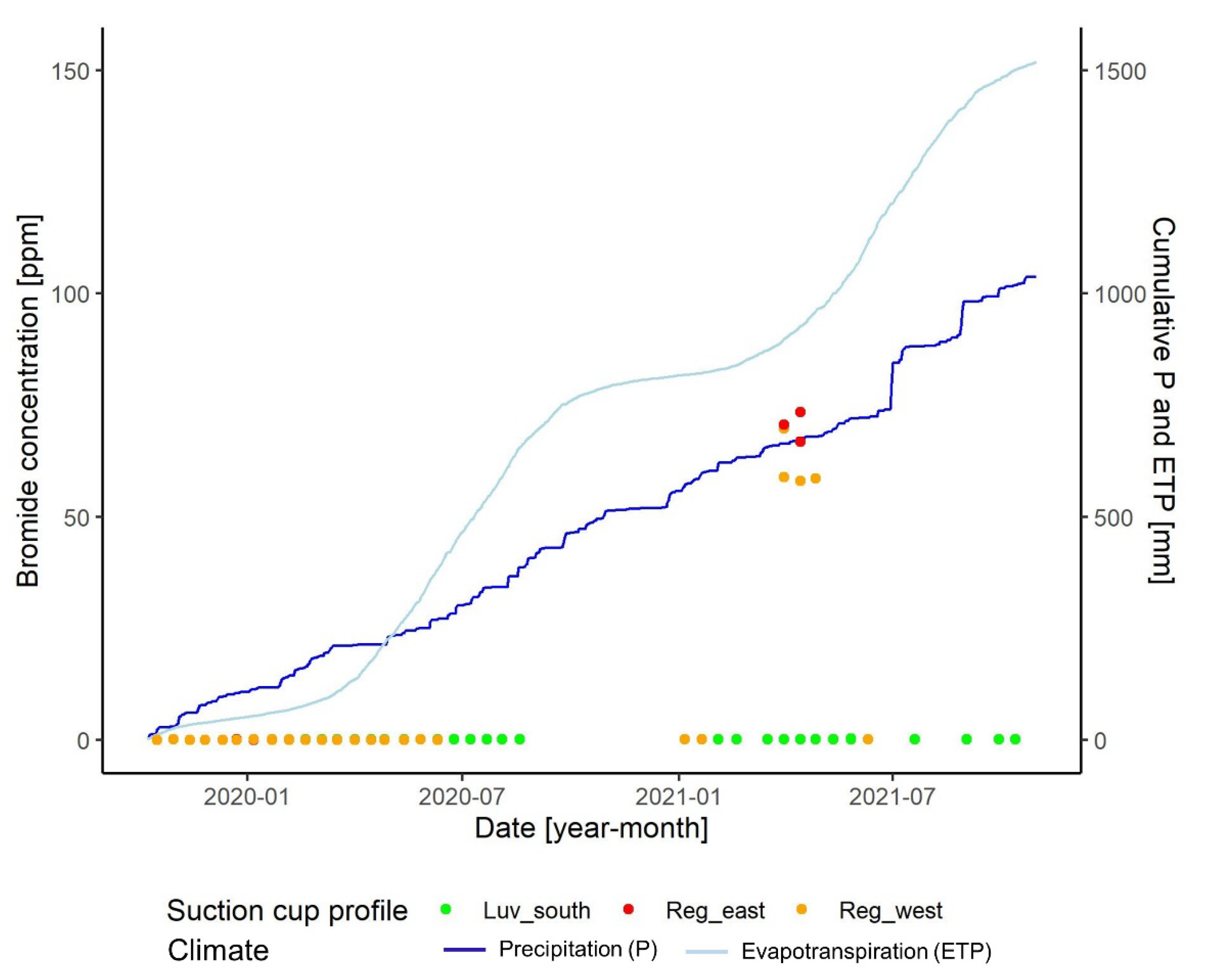
2.3. Tracer Monitoring

Soil sampling was carried out with a Pürckhauer soil probe along 3 profiles perpendicular to the former tracer application trench down to 1 m depth on March 29 at the Luvisol plot and on 1 April 2021 at the Regosol plot. The profiles were located at 1.5 m, 5 m, and 8.5 m along the trench. At each profile, two core samples were taken at 1 m, 0.5 m uphill from the trench, inside the trench (0 m), and 0.5 m, 1 m, and 1.5 m downhill from the trench (Appendix A, Figure A1, and Figure A2). At each sampling point, two soil probes were subdivided into 10 cm increments down to 1 m depth similar to [28]. The samples at one sampling point and similar depths from the two soil probes were mixed to obtain sufficient soil mass for the analysis. The mixed soil samples were weighed before and after drying at 105 °C for 24 h in the laboratory to obtain field water content (Equation (3)). Approx. 50 g of the dry soil samples were equilibrated with 150 mL of deionized water and placed for 2 h into a rotating shaker and afterwards left for sedimentation for 5 h. The supernatant was filtered through filter paper (Filtrak folded filter, quality 389, pore size: 20 µm, Freiberg Zellstoff- und Papierfabrik zu Weissenborn) for approx. 20 h. 100 mL of the filtrate was mixed for 5 min on a magnetic stirrer with 10 mL KNO₃ (1M)–ISA-solution to buffer the influence of non-bromide-ions on the measurements [29]. The obtained soil solution was analysed with the ion-selective Bromide-electrode DX280 (Mettler-Toledo GmbH, Gießen, Germany) in mmol l⁻¹ at 20 °C room temperature. Additionally, every 10th sample was measured with ion chromatography (882 Compact IC plus, Deutsche Metrohm GmbH & Co. KG) for comparison and verification of the electrode measurements. The concentration of the extracted soil solution was converted from mmol Br⁻ l⁻¹ soil solution to mg Br⁻ kg⁻¹ soil. Background values of the extraction method were evaluated by applying the above-mentioned steps to deionized water without soil. The background value of the extraction method was subtracted from the measured Bromide concentration in each sample. For background values of the field soil, the soil was sampled within the respective depths within >20 m distance parallel to the tracer application trench.

Both sites are equipped with suction cups of which 5 are located at 40 cm depth. Three (Reg) to five (Luv) suction cups are installed at 160 cm depth. The suction cups are distributed over a distance of 630 cm (Luv) and 490 cm (Reg) perpendicular to the flow direction (Figure 1). The soil pore water solution was collected every two weeks if enough soil solution was available, and analysed for bromide (among other ions) by ion chromatography (882 Compact IC plus, Deutsche Metrohm GmbH & Co. KG)

2.4. 3D-Reconstruction of Soil Layering

The 3D visualisation of surface elevation and the lower boundaries of soil horizons was executed with Surfer 17.1.288; Golden Software, LLC (www.goldensoftware.com, accessed on 12 December 2022) [30]. The surface elevation was resampled from 18 reference soil core positions by minimum curvature interpolation of the extracted values from the 1 m Laser-DEM of the state of Brandenburg to a 10 cm × 10 cm grid. Lower boundaries of the soil horizons were also interpolated by a minimum curvature approach to smooth the gridded surfaces (50 cm × 350 cm). Experimental design with the spatial reference point (fixed logger position), soil core positions, tracer trench, and suction cup positions were visualized using ArcGIS Map 10.6.1. (ESRI Inc. 1999–2017) [31].

3. Results

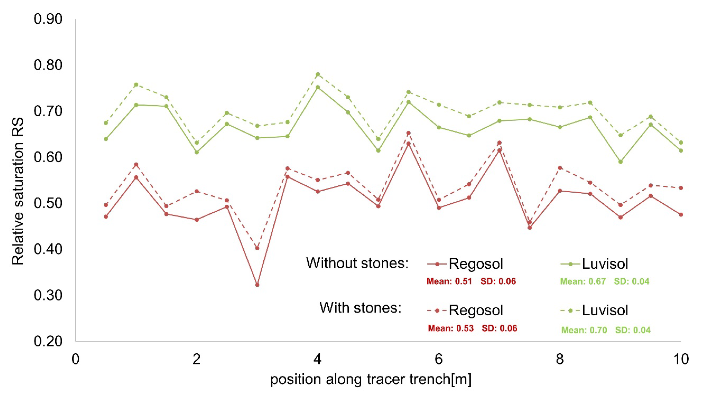
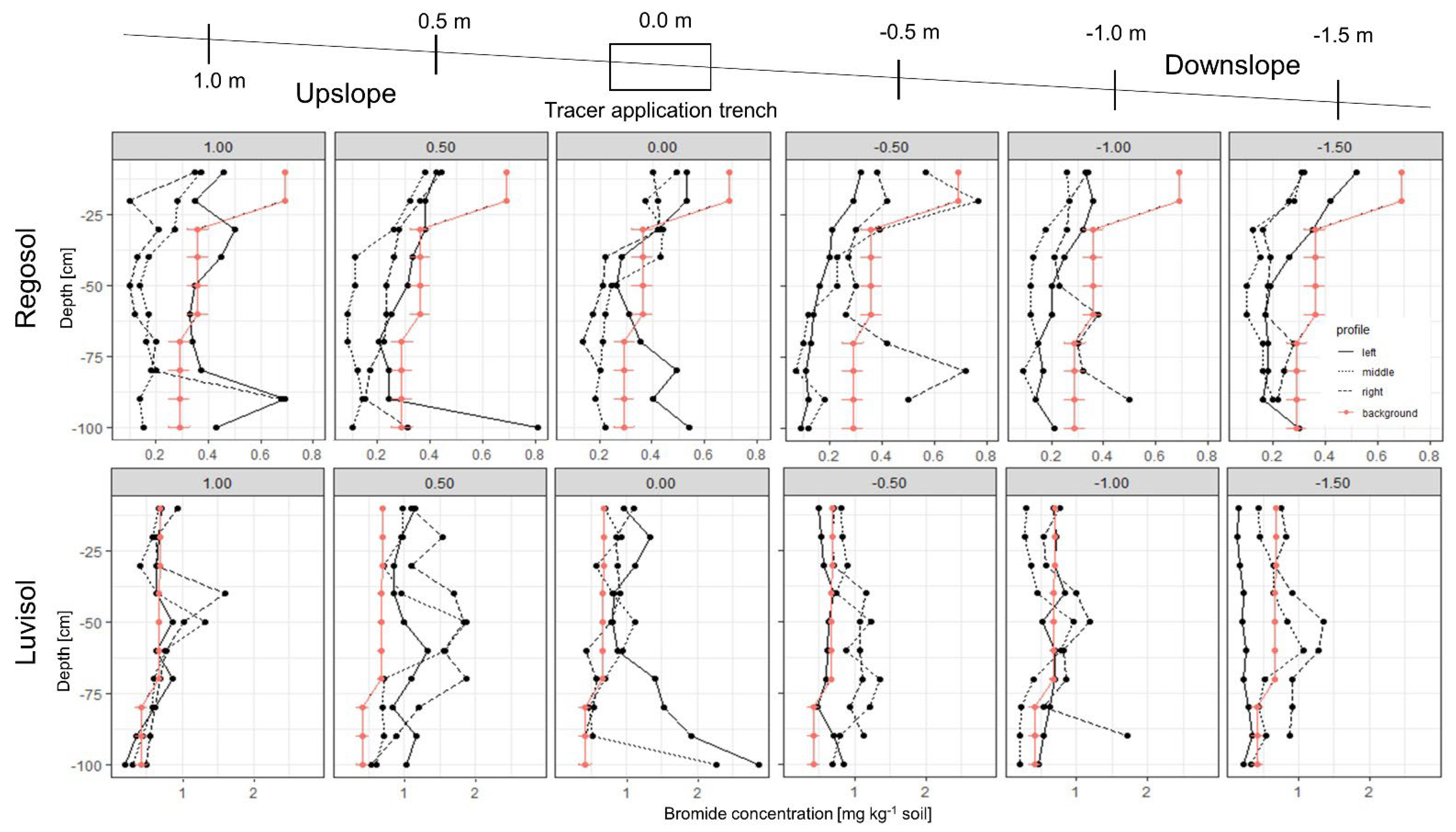
3.1. Tracer Concentration Observation and Relative Saturation along the Tracer Application Trench

The tracer was recovered by the suction cups in the Regosol after 663 mm of cumulative rainfall and 898 mm of cumulative evapotranspiration (Figure 3).

The relative saturation varied along the tracer application trench (Figure 4). For the Luvisol soil, the relative saturation with and without stones varied between 0.65 and 0.8, whereas the Regosol showed a range relative saturation from 0.4 to 0.65. Less variation in relative saturation is observed for Luvisol in comparison to Regosol. The relative saturation is generally higher in the Luvisol than in the Regosol and with stones than without stones. Analysis of the semivariance indicated that the measurements are spatially independent of each other (sample variance 0.003% and 0.002% for the Regosol and Luvisol, respectively). Values for the bulk density and water content can be found in Appendix A,

Table A1. Water content θ [g g⁻¹], bulk density ρ_b [g cm⁻³], effective porosity PV [-] and relative saturation S_e[-] of the regosol and the luvisol along the tracer application trench during the tracer application on 8 and 9 October 2019.

Position Along Tracer Trench [m]	Without Stones								With Stones
	θ [g/g]		ρ [g/cm 3]		PV [-]		Se [-]		θ [g/g]		ρ [g/cm 3]		PV [-]		Se [-]
	Reg	Luv	Reg	Luv	Reg	Luv	Reg	Luv	Reg	Luv	Reg	Luv	Reg	Luv	Reg	Luv
0.5	0.18	0.24	1.64	1.64	0.38	0.38	0.47	0.64	0.18	0.24	1.69	1.69	0.36	0.36	0.50	0.67
1	0.19	0.25	1.74	1.70	0.34	0.36	0.56	0.71	0.19	0.25	1.78	1.76	0.33	0.34	0.58	0.76
1.5	0.19	0.25	1.61	1.71	0.39	0.35	0.48	0.71	0.19	0.25	1.65	1.74	0.38	0.34	0.49	0.73
2	0.19	0.24	1.58	1.61	0.41	0.39	0.46	0.61	0.19	0.24	1.70	1.64	0.36	0.38	0.53	0.63
2.5	0.19	0.25	1.64	1.66	0.38	0.37	0.49	0.67	0.19	0.25	1.67	1.70	0.37	0.36	0.51	0.70
3	0.16	0.25	1.37	1.63	0.48	0.38	0.32	0.64	0.16	0.25	1.63	1.67	0.39	0.37	0.40	0.67
3.5	0.20	0.25	1.70	1.62	0.36	0.39	0.56	0.65	0.20	0.25	1.73	1.67	0.35	0.37	0.58	0.68
4	0.20	0.27	1.64	1.70	0.38	0.36	0.53	0.75	0.20	0.27	1.69	1.73	0.36	0.35	0.55	0.78
4.5	0.20	0.26	1.69	1.66	0.36	0.37	0.54	0.70	0.20	0.26	1.73	1.70	0.35	0.36	0.57	0.73
5	0.19	0.25	1.61	1.58	0.39	0.40	0.49	0.61	0.19	0.25	1.63	1.62	0.38	0.39	0.51	0.64
5.5	0.21	0.25	1.77	1.72	0.33	0.35	0.63	0.72	0.21	0.25	1.80	1.75	0.32	0.34	0.65	0.74
6	0.19	0.25	1.60	1.64	0.40	0.38	0.49	0.67	0.19	0.25	1.63	1.71	0.38	0.35	0.51	0.71
6.5	0.19	0.25	1.64	1.64	0.38	0.38	0.51	0.65	0.19	0.25	1.70	1.70	0.36	0.36	0.54	0.69
7	0.21	0.25	1.75	1.66	0.34	0.37	0.62	0.68	0.21	0.25	1.78	1.72	0.33	0.35	0.63	0.72
7.5	0.18	0.25	1.57	1.68	0.41	0.37	0.45	0.68	0.18	0.25	1.60	1.72	0.40	0.35	0.46	0.71
8	0.19	0.25	1.68	1.66	0.36	0.37	0.53	0.67	0.19	0.25	1.77	1.72	0.33	0.35	0.58	0.71
8.5	0.19	0.24	1.66	1.73	0.37	0.35	0.52	0.69	0.19	0.24	1.71	1.78	0.36	0.33	0.55	0.72
9	0.19	0.23	1.61	1.63	0.39	0.38	0.47	0.59	0.19	0.23	1.66	1.72	0.37	0.35	0.50	0.65
9.5	0.20	0.24	1.62	1.72	0.39	0.35	0.52	0.67	0.20	0.24	1.67	1.74	0.37	0.34	0.54	0.69
10	0.19	0.22	1.59	1.70	0.40	0.36	0.48	0.61	0.19	0.22	1.70	1.73	0.36	0.35	0.53	0.63

.

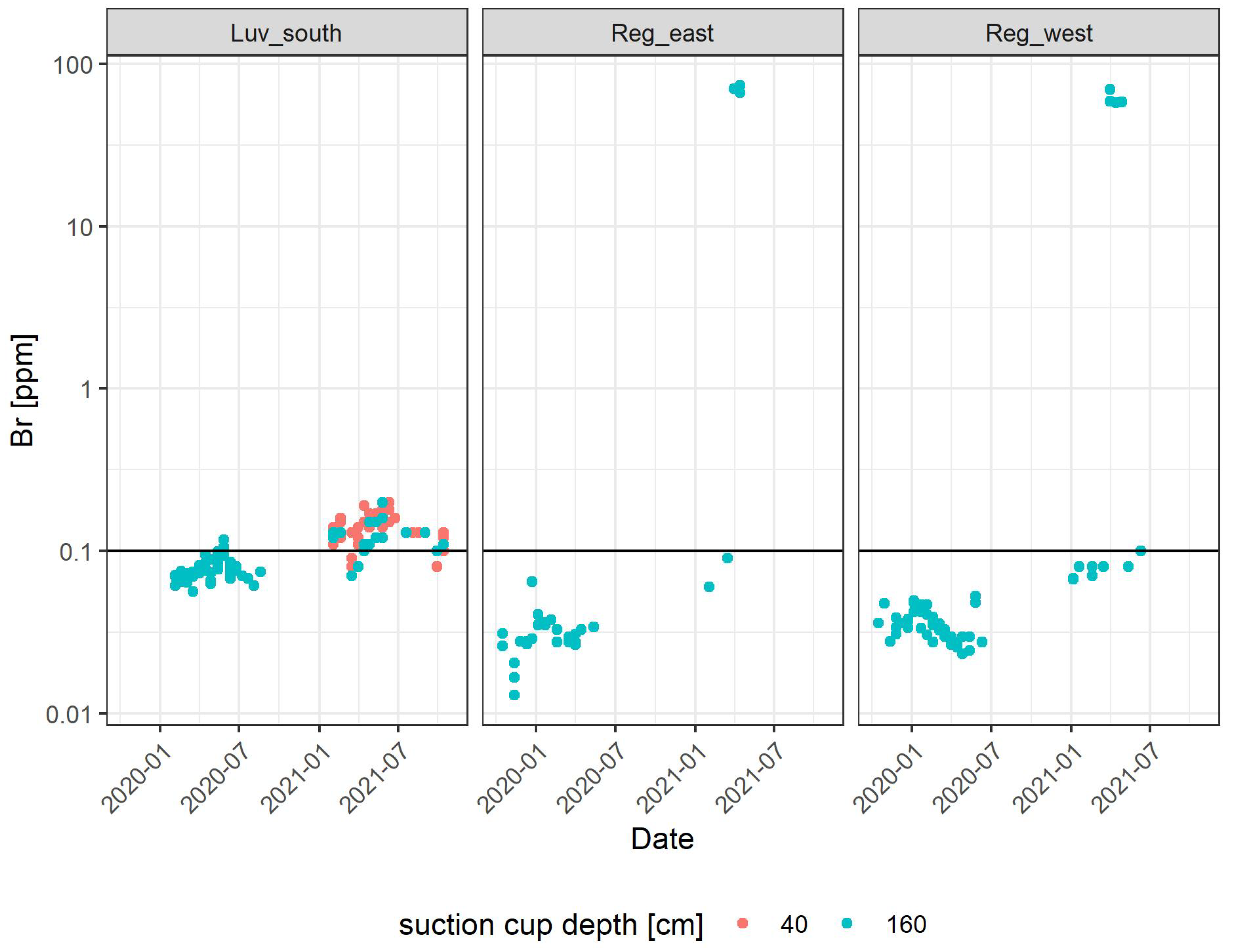
3.2. Bromide Concentration in Soil Pore Water (Suction Cup Measurements)

Bromide concentrations in the pore water of the Luvisol stayed in most cases below the background value of 0.1 ppm throughout the observation period from October 2019 to October 2021 (Figure 5, left). A slight increase of Bromide concentration above the background value was observed at 160 cm depth in spring 2021. Most measurements were taken at 160 cm depth. In other depths, no soil water could be sampled due to dry weather conditions. Only throughout the precipitation maxima in the summer of 2020 (Figure 2), sampling was also possible closer to the surface (Figure 5). Due to drought conditions, even in 160 cm soil depth, no sampling of pore water was possible in the summer/autumn of 2019 and 2020.

At the Regosol site bromide pore water concentrations stayed below the background value at 40 and 160 cm depth until the beginning of March 2021 (Figure 5, right). First elevated concentrations of bromide were recorded at 160 cm depth on 31 March 2021. The bromide was detected at both suction cup profiles, the one located at the western part (Reg_west) and the eastern part (Reg_east) of the Regosol plot directly below the application trench. Bromide concentrations in the eastern part were on average higher (68–73 ppm) than in the western part of the Regosol plot (58–70 ppm) indicating a northwestern flow direction (Figure 3). For the eastern part of the plot, soil conditions were too dry to sample after 14 April 2021. In the western part of the Regosol plot elevated bromide concentrations were measured until 27 April 2021 and declined below the background value until 12 May 2021.

3.3. Bromide Concentration in Soil Samples

One and a half years after the tracer application almost no bromide-ions were found at the Regosol site 1 m uphill and 1.5 m downhill from the tracer application trench (Figure 6, top). Most measured concentrations are lower than the background values of the soil in the respective depths. For the Regsol site, Bromide concentrations varied between 0.1 and 0.8 mg Br⁻ kg⁻¹ soil. A reduction of Br⁻-concentrations from the top layers to the bottom layers is observed indicating atmospheric deposition. The left and middle profiles at the Regosol site show slightly increased Br⁻-concentrations at depths >75 cm. Since the measurements of the Bromide ion-selective electrode are not assessable at concentrations <1 mg Br⁻ kg⁻¹ soil, these values might be attributed to measurement uncertainties. Furthermore, due to limited sampling material, only one measurement per sampling depth was possible limiting the error assessment of the measurements.

The Luvisol profiles show slightly elevated Br⁻-concentrations or concentrations within the range of the background values for the respective depths (Figure 6, bottom). Br⁻ -concentrations for the Luvisol site vary between 0.5 and 3 mg Br⁻ kg⁻¹ soil. At the tracer application trench a strong increase of Br⁻-concentrations is found in depth > 60 cm, indicating a vertical infiltration of the tracer. Unlike the Regosol site no elevated Br⁻-concentrations are found in the upper 30 cm of the soil. Br⁻-concentrations higher than the background value found in 30 to 50 cm upslope and 50 to 75 cm 1.5 m downslope the tracer application trench might indicate a plume-like distribution of the tracer right after the application in October 2019. Since too much time has passed this possible tracer distribution is not clearly visible anymore.

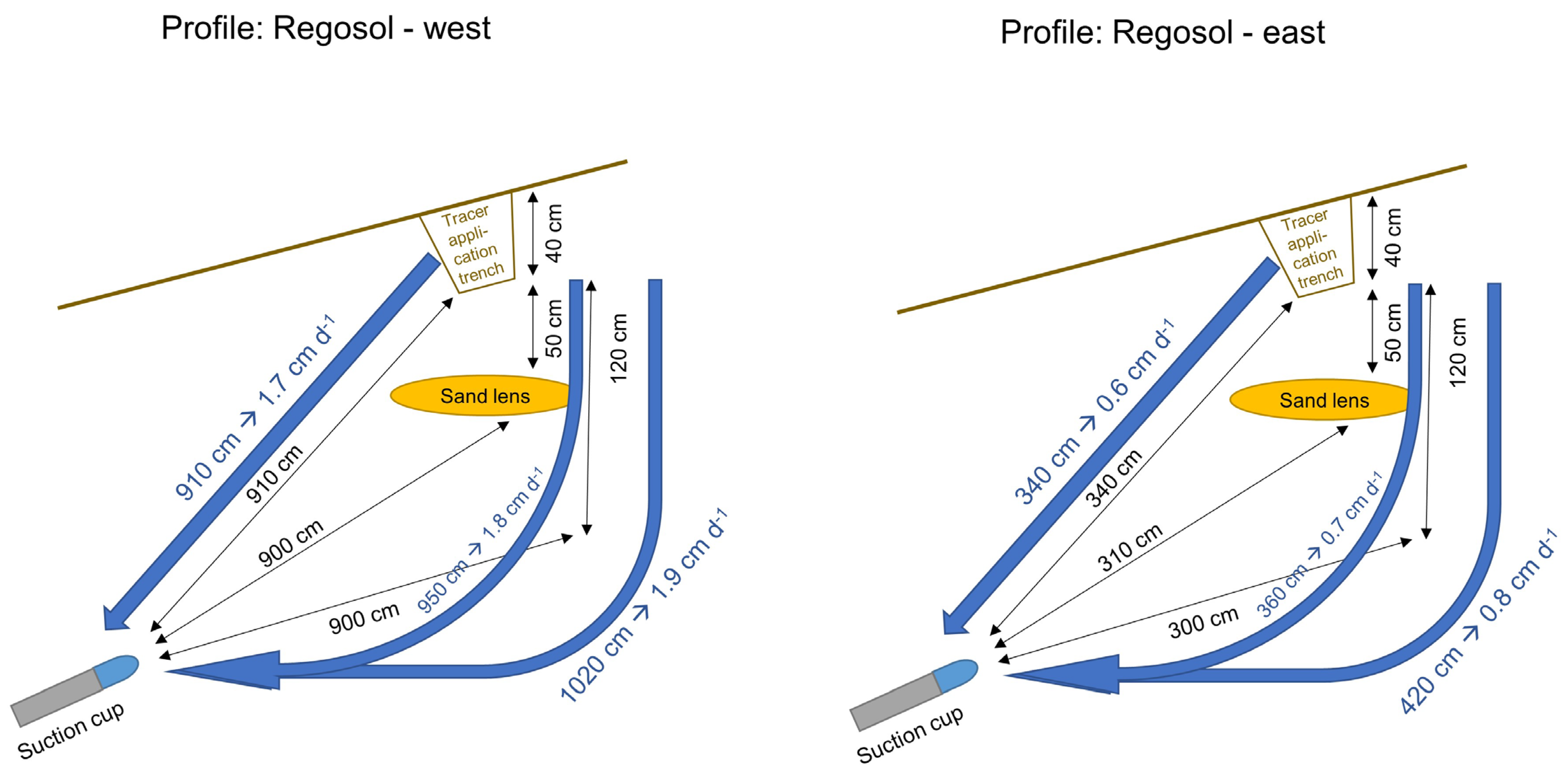
3.4. Estimated Transport Distances in Luvisol and the Regosol Soil Profiles

Elevated concentrations of Bromide were found in the Luvisol in 80–90 cm depth after 539 days (Figure 6). Average daily bromide transport distances per time could be estimated from the time difference between tracer injection and concentration peak in the suction cups and the distance covered by the tracer. Since no concentration peaks are found in the soil profile of the Luvisol several assumptions have to be made: after the tracer application, the bromide is dissolved in a depth of 40 cm and assimilated by plants or transported by the subsurface water flow. Due to the dispersion and diffusion process, the concentration front expands and the maximum concentration of bromide decreases. In the case of a homogeneous vertical transport, the concentration peak is found below 1 m soil depth (Figure 6). Thus, a vertical displacement of the tracer of at least 60 cm (1 m–0.4 m) is assumed. The transport distance of 60 cm for the period of 539 days is here given as a minimum flow and transport distance per day >0.11 m. The average transport distance is most likely higher since the concentration of bromide increases with depth and the actual flow paths are longer due to dispersion and diffusion phenomena.

For the Regosol no elevated Bromide concentrations were detected during the soil sampling at the end of March 2021 (Figure 6). However, the Bromide was found in the suction cup profiles at 160 cm depth 3 m downslope from the application trench in April 2021 (Figure 3). If a vertical infiltration is assumed with a lateral redirection of the water in 160 cm depth a minimum distance of 340 cm and a maximum distance of 420 cm was covered by the tracer within 541 days. This indicates a minimum transport distance per day from 0.6 to 0.8 cm (for assumptions see Figure 7, eastern profile). Moreover, the tracer was not only recovered in the suction cup profile directly downslope (eastern suction cup profile) but in the suction cup profile northwest of the application trench around the same time. In order to cover this distance the tracer must have travelled at least 9 to 10 m within this time indicating a minimum transport distance per day of 1.7 to 1.9 cm⁻ (for assumptions see Figure 7, western profile).

Thus the actual transport distance per day of the tracer could be between 0.6 and 1.9 cm.

Note that from these assumptions for the transport distance in the Regosol and Luvisol, it may be deduced that the tracer must have moved at least a certain distance in the soil from the first precipitation till the recovery of the tracer in the suction cups.

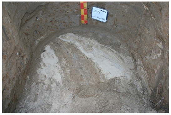
3.5. 3D-Reconstruction of Soil Layering and Flow Path Reconstruction

The reconstructed horizon boundaries in the subsurface do not correspond to the surface inclination (Figure 8). For example, the lower boundary of the Bgk1-horizon is shaped similar to a subsurface dell. Furthermore, a sand lens was discovered at the right part of the profile that did not extend towards the middle or left part of the reconstructed subsurface. The tracer was recovered at the eastern profile at 160 cm depth in the vicinity of the sand lens (Figure 8). Surprisingly, the bromide was also found at the eastern suction cup profile northeast of the application trench (Figure 8).

4. Discussion

4.1. Subsurface Flow Patterns in the Luvisol and Regosol

From October 2019 to the beginning of April 2021, the vertical flow was observed in the Luvisol, whereas lateral flow was found in the Regosol. The estimated transport distance in the Regosol was three to four times higher than in the Luvisol. When water infiltrates the soil it will infiltrate vertically under unsaturated conditions. However, when local saturation occurs along an impeding layer in the subsurface water might be redirected laterally. These transport patterns differ between Regosol and Luvisol. Only in the Regosol LSF occurred, whereas flow remained vertical in the Luvisol despite the expected occurrence of LSF along the clay-enriched Btg-horizon (Table 1).

One explanation for the differing assumed flow dynamics in the Luvisol and the Regosol might be the high earthworm activity in the Btg-horizon of the Luvisol (Appendix A, Figure A3) that enhances vertical infiltration through macropores [32]. In contrast, small sand bands in the heterogeneous structure of the Regosol might provide lateral preferential pathways (Appendix A, Figure A4). Furthermore, during the soil sampling with the Pürckhauer soil probe a sand lens was discovered at approximately 90 cm depth (Figure 8). This might have led to LSF as observed by Walter et al. [33] along sand lenses or by Robinson et al. [22] within a sandy layer towards a drainage ditch. In our case, a subsurface flow might be related to the somehow erratic occurrence of sand lenses or sand bands within the glacial till which are not necessarily layered or regularly distributed within the area (note: glacial till is a mixed, massive, non-layered material from glacial deposits). Soil profiling (11 soil core positions, not shown) in the surrounding of 25 m indicates sandy material varying in depths from 30 to 180 cm to no sand at all (four positions).

4.2. Flow Patterns, Conditions, and Depth of LSF Occurrence

Flow patterns in the Luvisol and Regosol are irregular and represent the heterogeneous soil structure. For example, in the Luvisol the bromide concentrations in vertical directions differ among the three sampling positions in the left, right and middle part along the tracer application trench (Figure 6): Just below the trench (0.0 m) the profile in the left part of the application trench shows increased bromide concentrations from 60 cm depth, whereas the profile in the middle shows only higher bromide concentrations in 100 cm depth. Furthermore, 1.5 m downslope from the trench the profiles in the middle and right part of the trench show higher bromide concentrations in 50–60 cm depth, in contrast to the concentrations of the left profile that stay just below the background concentration. Similarly, in the Regosol, not all five suction cups installed at 160 cm depth showed increased bromide concentrations (Figure 8), since not all suction cups received enough water to draw samples. This might be attributed to the heterogeneous initial relative saturation during the tracer application (Figure 4): In areas with higher initial water content, the tracer might dissolve faster and thus be transported faster than in areas with smaller initial water content [34]. In addition, the subsurface exhibits a very heterogeneous structure (Figure 8) that enhances heterogeneous flow patterns, e.g., via preferential flow paths. With techniques such as ground penetrating radar [35] or areal electrical resistivity imaging (ERI) [22] it might be possible to reveal these preferential flow pathways.

In the Regosol the bromide tracer was recovered 3 m downslope from the application trench after 668 mm of cumulative rainfall. A similar amount of cumulative rainfall (700 mm) for the relocation of the tracer over the same distance but in a vertical direction and loamy sand soil under agricultural use was found by Bero et al. [18]. In contrast to that, Logsdon [20] recovered the bromide tracer 3 m downslope from its application trench after only 256 mm of cumulative rainfall in a fine loamy glacial till the soil, despite smaller saturated conductivities in a horizontal direction (9–32 cm d⁻¹) compared to the Regosol of this study (Table 1). However, in the study of Logsdon [20] the tracer was recovered already after 5 months, whereas in the present study almost 17 months passed before the tracer was found. Drying periods might have slowed the tracer movement or even reverted the flow direction towards the soil surface due to evaporation. In forest soils, the transport of the tracer over larger distances was observed already at much less cumulative rainfall: Anderson et al. [15] reported a total of 179 mm and 376 mm rainfall for a NaCl tracer to be transported 12 m and 30 m downslope, respectively.

Lateral movement of the bromide tracer was observed at 160 cm depth in the Regosol (Figure 5), whereas for the Luvisol it remains unclear whether there is a lateral distribution of the bromide or not. After 1.5 years, the tracer was recovered at 70 to 100 cm depth just below the tracer application trench in the Luvisol (Figure 6), indicating a much smaller transport distance than in the Regosol. However, the tracer plume might have bypassed the suction cups located 3 m downslope of the application trench, since the cups were only installed at 40 and 160 cm depth. For example, Logsdon [20] recovered the tracer in a similar glacial till the soil at a 60 cm depth, 3 m downslope from the tracer application trench. They suggest that the depth of the groundwater table might influence the lateral tracer transport: LSF might occur in the capillary fringe of the groundwater table or the upper part of the saturated zone. However, the lateral tracer movement at 160 cm depth in the current study is supported by the numerical predictions of Filipović et al. [9]. In their modelling study of a similar soil as in this field experiment, lateral tracer distribution was reported along the Btg-CBkg horizon boundary at 150–160 cm depth.

4.3. Subsurface Lateral Tracer Transport Distances

The observed transport distances per day of >0.11 cm and 0.6 to 1.9 cm for the Luvisol and the Regosol, respectively, are well within range as compared to tracer studies in agricultural landscapes. Bero et al. [8] found transport distances per day ranging from 1.25 to 1.7 cm in a loamy sand soil of an agricultural hillslope, similar to the transport distances per day of the Regosol in this study. In their simulations, Filipović et al. [9] observed lateral flow and transport along a distance of approximately 50 cm after the first rainfall event 100 d after the tracer application resulting in an average transport distance per day of 0.5 cm. This average transport distance lies between the vertical transport distance of the Luvisol and the lateral transport distance of the Regosol in this study. In contrast, Köhne & Gerke [36] reported much higher transport distances per day, around 175 cm (the tracer was recovered 35 m downslope from the application site after 20 days) in a tile-drained glacial till field. However, they applied the tracer by irrigation, which enhances the initial transport artificially.

Bathke et al. [21] carried out a similarly designed experiment in a sandy clay loam over saprolite under pasture. They applied the tracer as a solid substance under natural rainfall. Similar to the study of Filipović et al. [9], they observed transport distances per day between 0.3 and 0.6 cm, well within the range of our study. Thus, transport distances observed under natural precipitation conditions are found to be smaller than in studies, where the tracer is applied as a solution [18,36]. This underlines the importance of tracer application as a solid substance when analysing transport times of nutrients or pesticides in the field. From the still limited number of tracer studies in agricultural landscapes as well as considering the data situation of this study, conclusions about average flow and transport distances seem to be not yet reliable.

5. Conclusions

The aims of this study were to identify the phenomenon of LSF in agricultural field soils, analyze the influence of subsurface soil structure on LSF, and estimate vertical and lateral subsurface transport pathways.

Despite smaller bulk densities and higher saturated hydraulic conductivities, observed transport pathways in the Luvisol indicate a mainly vertically directed infiltration pattern. For the Regosol, LSF was observed at 160 cm depth, but not in all suction cups installed over a distance of five meters. These highly heterogeneous flow patterns are related to a heterogeneous soil structure providing preferential flow pathways, e.g., via sand bands in rather compacted soil glacial till horizons in the soils of the hummocky ground moraine. These results indicate that quantification of LSF phenomena remains a challenge; results are highly dependent on the soil subsurface heterogeneities. Here, soil sampling below 1 m or a model-based pre-assessment of flow pathways could have helped to improve and reduce sampling effort.

A better characterisation of the subsurface in combination with a model-based pre-assessment of subsurface flow pathways might have improved the timing and spacing of the soil sampling. This underlines the importance of assessing subsurface soil structures and flow pathways for better predicting the occurrence of LSF. Nevertheless, LSF seems to occur even under rather dry climate conditions and remains an important transport process even under changing climatic conditions.

References

1. Kalettka, T.; Rudat, C. Hydrogeomorphic types of glacially created kettle holes in North-East Germany. Limnologica 2006, 36, 54–64. [Google Scholar] [CrossRef] [Green Version]
2. Jarvis, N.; Koestel, J.; Larsbo, M. Understanding Preferential Flow in the Vadose Zone: Recent Advances and Future Prospects. Vadose Zone J. 2016, 15, 1–11. [Google Scholar] [CrossRef]
3. Xie, M.; Šimůnek, J.; Zhang, Z.; Zhang, P.; Xu, J.; Lin, Q. Nitrate subsurface transport and losses in response to its initial distributions in sloped soils: An experimental and modelling study. Hydrol. Process. 2019, 33, 3282–3296. [Google Scholar] [CrossRef]
4. Cueff, S.; Alletto, L.; Bourdat-Deschamps, M.; Benoit, P.; Pot, V. Water and pesticide transfers in undisturbed soil columns sampled from a Stagnic Luvisol and a Vermic Umbrisol both cultivated under conventional and conservation agriculture. Geoderma 2020, 377, 114590. [Google Scholar] [CrossRef]
5. Guo, L.; Lin, H. Addressing Two Bottlenecks to Advance the Understanding of Preferential Flow in Soils; Elsevier: Amsterdam, The Netherlands, 2018; pp. 61–117. ISBN 9780128152836. [Google Scholar]
6. Scaini, A.; Audebert, M.; Hissler, C.; Fenicia, F.; Gourdol, L.; Pfister, L.; Beven, K.J. Velocity and celerity dynamics at plot scale inferred from artificial tracing experiments and time-lapse ERT. J. Hydrol. 2017, 546, 28–43. [Google Scholar] [CrossRef]
7. Gerke, K.M.; Sidle, R.C.; Mallants, D. Preferential flow mechanisms identified from staining experiments in forested hillslopes. Hydrol. Process. 2015, 29, 4562–4578. [Google Scholar] [CrossRef]
8. Luo, Z.; Niu, J.; Xie, B.; Zhang, L.; Chen, X.; Berndtsson, R.; Du, J.; Ao, J.; Yang, L.; Zhu, S. Influence of Root Distribution on Preferential Flow in Deciduous and Coniferous Forest Soils. Forests 2019, 10, 986. [Google Scholar] [CrossRef] [Green Version]
9. Filipović, V.; Gerke, H.H.; Filipović, L.; Sommer, M. Quantifying Subsurface Lateral Flow along Sloping Horizon Boundaries in Soil Profiles of a Hummocky Ground Moraine. Vadose Zone J. 2018, 17, 1–12. [Google Scholar] [CrossRef] [Green Version]
10. Ehrhardt, A.; Groh, J.; Gerke, H.H. Wavelet analysis of soil water state variables for identification of lateral subsurface flow: Lysimeter vs. field data. Vadose Zone J. 2021, 20, 149. [Google Scholar] [CrossRef]
11. Hardie, M.A.; Doyle, R.B.; Cotching, W.E.; Lisson, S. Subsurface Lateral Flow in Texture-Contrast (Duplex) Soils and Catchments with Shallow Bedrock. Appl. Environ. Soil Sci. 2012, 2012, 861358. [Google Scholar] [CrossRef] [Green Version]
12. Sander, T.; Gerke, H.H. Preferential Flow Patterns in Paddy Fields Using a Dye Tracer. Vadose Zone J. 2007, 6, 105–115. [Google Scholar] [CrossRef]
13. Kung, K.S.J. Preferential flow in a sandy vadose zone: 1. Field observation. Geoderma 1990, 46, 51–58. [Google Scholar] [CrossRef]
14. Ehrhardt, A.; Berger, K.; Filipović, V.; Wöhling, T.; Vogel, H.-J.; Gerke, H.H. Tracing lateral subsurface flow in layered soils by undisturbed monolith sampling, targeted laboratory experiments, and model-based analysis. Vadose Zone J. 2022, 21, 1075. [Google Scholar] [CrossRef]
15. Anderson, A.E.; Weiler, M.; Alila, Y.; Hudson, R.O. Subsurface flow velocities in a hillslope with lateral preferential flow. Water Resour. Res. 2009, 45, 1043. [Google Scholar] [CrossRef] [Green Version]
16. Koch, J.C.; Toohey, R.C.; Reeves, D.M. Tracer-based evidence of heterogeneity in subsurface flow and storage within a boreal hillslope. Hydrol. Process. 2017, 31, 2453–2463. [Google Scholar] [CrossRef]
17. Laine-Kaulio, H.; Koivusalo, H. Model-based exploration of hydrological connectivity and solute transport in a forested hillslope. Land Degrad. Dev. 2018, 29, 1176–1189. [Google Scholar] [CrossRef]
18. Bero, N.J.; Ruark, M.D.; Lowery, B. Bromide and chloride tracer application to determine sufficiency of plot size and well depth placement to capture preferential flow and solute leaching. Geoderma 2016, 262, 94–100. [Google Scholar] [CrossRef]
19. Gerke, H.H.; Maximilian Köhne, J. Dual-permeability modeling of preferential bromide leaching from a tile-drained glacial till agricultural field. J. Hydrol. 2004, 289, 239–257. [Google Scholar] [CrossRef]
20. Logsdon, S.D. Subsurface lateral transport in glacial till soils. Trans. ASABE 2007, 50, 875–883. [Google Scholar] [CrossRef]
21. Bathke, G.R.; Cassel, D.K.; McDaniel, P.A. Bromide movement at selected sites in a dissected Piedmont landscape. J. Environ. Qual. 1992, 21, 469–475. [Google Scholar] [CrossRef]
22. Robinson, J.; Buda, A.; Collick, A.; Shober, A.; Ntarlagiannis, D.; Bryant, R.; Folmar, G.; Andres, S.; Slater, L. Electrical monitoring of saline tracers to reveal subsurface flow pathways in a flat ditch-drained field. J. Hydrol. 2020, 586, 124862. [Google Scholar] [CrossRef]
23. Boeing, F.; Rakovec, O.; Kumar, R.; Samaniego, L.; Schrön, M.; Hildebrandt, A.; Rebmann, C.; Thober, S.; Müller, S.; Zacharias, S.; et al. High-resolution drought simulations and comparison to soil moisture observations in Germany. Hydrol. Earth Syst. Sci. 2022, 26, 5137–5161. [Google Scholar] [CrossRef]
24. Zink, M.; Samaniego, L.; Kumar, R.; Thober, S.; Mai, J.; Schäfer, D.; Marx, A. The German drought monitor. Environ. Res. Lett. 2016, 11, 74002. [Google Scholar] [CrossRef]
25. Sommer, M.; Augustin, J.; Kleber, M. Feedbacks of soil erosion on SOC patterns and carbon dynamics in agricultural landscapes—The CarboZALF experiment. Soil Tillage Res. 2016, 156, 182–184. [Google Scholar] [CrossRef]
26. Gerke, H.H.; Koszinski, S.; Kalettka, T.; Sommer, M. Structures and hydrologic function of soil landscapes with kettle holes using an integrated hydropedological approach. J. Hydrol. 2010, 393, 123–132. [Google Scholar] [CrossRef]
27. Rieckh, H.; Gerke, H.H.; Sommer, M. Hydraulic properties of characteristic horizons depending on relief position and structure in a hummocky glacial soil landscape. Soil Tillage Res. 2012, 125, 123–131. [Google Scholar] [CrossRef]
28. Kahl, G.; Ingwersen, J.; Nutniyom, P.; Totrakool, S.; Pansombat, K.; Thavornyutikarn, P.; Streck, T. Micro-trench experiments on interflow and lateral pesticide transport in a sloped soil in northern Thailand. J. Environ. Qual. 2007, 36, 1205–1216. [Google Scholar] [CrossRef] [PubMed]
29. Mettler Toledo. Operating: Operating Instruction for Br-Ion-Selective Electrode; Mettler Toledo: Greifensee, Switzerland.
30. Surfer Grapher. Surfer (Version 17.1.288; 64-bit); Golden Software, LLC.: Golden, CO, USA, 2019. [Google Scholar]
31. ESRI Inc. ArcGIS Map (Version 10.6.1); ESRI Inc.: Redlands, CA, USA, 2017. [Google Scholar]
32. Leue, M.; Uteau, D.; Peth, S.; Beck-Broichsitter, S.; Gerke, H.H. Volume-related quantification of organic carbon content and cation exchange capacity of macropore surfaces in Bt horizons. Vadose Zone J. 2020, 19, e20069. [Google Scholar] [CrossRef]
33. Walter, M.T.; Kim, J.-S.; Steenhuis, T.S.; Parlange, J.-Y.; Heilig, A.; Braddock, R.D.; Selker, J.S.; Boll, J. Funneled flow mechanisms in a sloping layered soil. Water Resour. Res. 2000, 36, 841–849. [Google Scholar] [CrossRef] [Green Version]
34. McCord, J.T.; Stephens, D.B. Lateral moisture flow beneath a sandy hillslope without an apparent impeding layer. Hydrol. Process. 1987, 1, 225–238. [Google Scholar] [CrossRef]
35. Guo, L.; Fan, B.; Zhang, J.; Lin, H. Occurrence of subsurface lateral flow in the Shale Hills Catchment indicated by a soil water mass balance method. Eur. J. Soil Sci. 2018, 69, 771–786. [Google Scholar] [CrossRef]
36. Köhne, J.M.; Gerke, H.H. Spatial and Temporal Dynamics of Preferential Bromide Movement towards a Tile Drain. Vadose Zone J. 2005, 4, 79–88. [Google Scholar] [CrossRef]
Figure 1. Map of the study site with the two tracer application sites at the Luvisol (Luv) and the Regosol (Reg). Suction cup profiles are located in the north (N), south (S), west (W), or east (E) of the respective plots. Assumed subsurface flow directions are indicated by arrows.
Water 15 01248 g001
Figure 2. Daily precipitation (blue line) and average daily temperatures (red line) at the study site from 10 August 2019 to 31 October 2021.
Water 15 01248 g002
Figure 3. Cumulative precipitation P (dark blue line) [mm], cumulative potential evapotranspiration ETP (light blue line) [mm], and bromide concentrations (dots) at the suction cup profiles (40 and 160 cm depth) during the period from 8 October 2019 to 31 October 2021 (see Figure 2) of the Regosol and Luvisol. A total of 1038 mm of precipitation was recorded within this period.
Water 15 01248 g003
Figure 4. Relative saturation along the tracer application trenches of the Luvisol (LP12) and the Regosol (LP7).
Water 15 01248 g004
Figure 5. Bromide concentrations in ppm were measured in the suction cup profiles 3 m downhill from the tracer application trench. The horizontal black line indicates the background value of the two profiles measured in the period from 2010 to 2013. The detection limit is 0.05 ppm. Note that the detection limit for Bromide in the suction cup sampling is smaller than in the measurements with the ion-sensitive electrode.
Water 15 01248 g005
Figure 6. Bromide concentrations (mg Br kg−1 soil) 1.0 m, 0.5 m above, in and 0.5, 1.0, and 1.5 m below the tracer application trench for the Regosol and Luvisol site. Red lines are background concentrations: note that these were determined on a single profile on the respective soils with two to three replicates in each horizon. Note the different scales for concentration in Luvisol and Regosol.
Water 15 01248 g006
Figure 7. Assumptions for the travel distances of the estimated flow paths (blue arrows) and derived average travel distances per day of the tracer for the Regosol west (left side) and Regosol east (right side). The three pathways reflect the shortest, the medium, and a relatively long subsurface flow path. Due to the phenomena of dispersion and diffusion, actual flow paths might even be longer than assumed in this sketch.
Water 15 01248 g007
Figure 8. A 3D-reconstruction of the subsurface around the tracer application trench and positions along the suction cup profile, where the Bromide tracer arrived at 160 cm depth. Green and pink stars indicate the suction cup positions where the tracer was recovered.
Water 15 01248 g008