Article

Improving Groundwater Imputation through Iterative Refinement Using Spatial and Temporal Correlations from In Situ Data with Machine Learning

1
Department of Civil and Construction Engineering, Brigham Young University, Provo, UT 84602, USA
2
Department of Geological Sciences, Brigham Young University, Provo, UT 84602, USA
*
Author to whom correspondence should be addressed.
Water 2023, 15(6), 1236; https://doi.org/10.3390/w15061236
Submission received: 19 February 2023 / Revised: 14 March 2023 / Accepted: 17 March 2023 / Published: 22 March 2023
(This article belongs to the Section Hydrogeology)

Abstract

:
Obtaining and managing groundwater data is difficult as it is common for time series datasets representing groundwater levels at wells to have large gaps of missing data. To address this issue, many methods have been developed to infill or impute the missing data. We present a method for improving data imputation through an iterative refinement model (IRM) machine learning framework that works on any aquifer dataset where each well has a complete record that can be a mixture of measured and input values. This approach corrects the imputed values by using both in situ observations and imputed values from nearby wells. We relied on the idea that similar wells that experience a similar environment (e.g., climate and pumping patterns) exhibit similar changes in groundwater levels. Based on this idea, we revisited the data from every well in the aquifer and “re-imputed” the missing values (i.e., values that had been previously imputed) using both in situ and imputed data from similar, nearby wells. We repeated this process for a predetermined number of iterations—updating the well values synchronously. Using IRM in conjuncture with satellite-based imputation provided better imputation and generated data that could provide valuable insight into aquifer behavior, even when limited or no data were available at individual wells. We applied our method to the Beryl-Enterprise aquifer in Utah, where many wells had large data gaps. We found patterns related to agricultural drawdown and long-term drying, as well as potential evidence for multiple previously unknown aquifers.

1. Introduction

1.1. Motivation

Groundwater is an important resource worldwide. In the United States, more than 40% of the population relies on groundwater as their primary source of drinking water [1]. Groundwater extraction has supported economic growth and social development, in-creased food security and mitigated the effects of drought in agricultural regions [2]. However, groundwater development has also depressed water tables [3], degraded ecosystems [4], and led to the deterioration of groundwater quality [5]. Although groundwater is considered a renewable resource, renewal rates vary greatly, and for many aquifers, significant extraction rates are not sustainable [6]. Therefore, to manage this resource effectively and sustainably, we needed methods to quantify groundwater changes at the aquifer level.
One challenge for characterizing historic aquifer behavior is that data at individual wells were generally sparse, with missing data and large time gaps between measurements, often with poor spatial coverage. In situ groundwater measurements at monitoring wells give a direct measure of groundwater conditions and provide important information about aquifer dynamics. These observations are obtained manually or by using data loggers. However, it is often the case that monitoring programs are curtained or that sensors break, resulting in gaps that can span from months to decades [7]. Insufficient groundwater level observation data make it difficult to assess the behavior of an aquifer, providing only limited information about groundwater availability and sustainability.
Groundwater has some unique attributes that facilitate its analysis. For example, groundwater levels are generally temporally autocorrelated, meaning that they follow seasonal patterns with a long-term trend [8]. Often, these seasonal patterns in agricultural areas result in groundwater levels that are highest in the spring immediately preceding the new irrigation season and are lowest in the fall at the end of the irrigation season, after which water levels exhibit some rebound during the winter months [9]. Depending on recharge, similar seasonal patterns can follow wet or dry periods. Groundwater is also spatially correlated, meaning that groundwater levels near an observation well tend to be similar, and changes at one well can affect groundwater levels in other parts of the aquifer. This has been shown to be particularly true when wells have similar usage [10]. Both temporal and spatial changes in groundwater are relatively slow compared to sampling frequency [11].
Despite these unique attributes, groundwater storage analysis comes with many challenges, and quantifying the availability of groundwater and the long-term impacts of climate variability on groundwater is more complex than for surface water [12]. Remote sensing techniques that automate the monitoring of other environmental processes do not accurately work on subsurface hydrology [13]. Even the newer gravity anomaly measurements by the Gravity Recovery and Climate Experiment (GRACE) sensors only track changes in total water storage and not changes in individual hydrologic components, though this sensor comes closest to measuring groundwater changes [14]. GRACE has a low spatial resolution (>150,000 km2), and its susceptibility to leakage (i.e., measurements in one pixel are affected by adjacent pixels) makes it challenging to use on small-to-medium-sized aquifers directly. Additionally, the lack of temporal history for GRACE data, only about 20 years, does not provide the context needed to understand groundwater storage changes over longer periods that are associated with processes such as development and climate change [15,16].
Recently there has been increasing interest in the characterization of groundwater using machine learning as an alternative to complicated physical models. In general, machine learning applied to groundwater issues is divided into three major groups: the performance comparison of different machine learning algorithms; imputing missing data values; and the simulation framework improvement [17]. Ahmadi et al. [18] compared the success of different machine learning algorithms on groundwater and showed that multi-layer perceptron models were used in 53% of published cases. In other examples, Vu et al. [19] used a temporal correlation between wells with an LSTM model to reconstruct groundwater level time series, though unreliable input caused poor predictions, and Bowes et al. [20] showed that precipitation data with an LSTM could be used to help with forecasts of the groundwater level response due to storm events in shallow costal aquifers.
Researchers have developed imputation methods to facilitate groundwater analysis using wells that have large gaps of missing data to improve traditional hydrogeological methods [21,22]. These approaches involve understanding the groundwater levels at individual wells and then using the point data with geostatistical methods such as K-nearest neighbors [23] or Kriging [24,25] to build monthly surfaces. The series of monthly surfaces can be analyzed to understand how groundwater storage may change in an aquifer or over a region [10]. For this approach to work, it was critical to have a complete dataset for the individual wells in the aquifer using the same time step with relatively dense spatial coverage [26,27].
Evans et al. [21] demonstrated that periods of missing groundwater observations could be imputed by regressing Earth observation data. They showed that each well had unique characteristics and interactions with precipitation and evapotranspiration that could be captured. This is based on the idea that during a drought, groundwater levels drop because there is less recharge and more groundwater pumping as surface water sources are reduced. Conversely, during a wet period, groundwater levels generally rise due to a net increase in recharge and reduced groundwater extraction as surface water resources are easier to exploit. However, each well behaves individually because of the local environment and well operations. They showed that, for imputation, a model should be developed for each well rather than developing a single aquifer-wide or regional model.
In our previous work, Ramirez et al. [22], we extended the Evans et al. [21] approach using an extended Self-Calibrated Dai Palmer Drought Severity Index PenmenMonteith (PDSI) and NASA’s Global Land Data Assimilation System (GLDAS) data as the meteorological features [22,28,29]. Our approach also created a model for each well within an aquifer but demonstrated significantly improved imputation results through the use of an inductive bias to build prior features for each well in the imputation process. We were able to demonstrate imputation over large 50-year gaps using this extended method.
Inductive bias is the general expectation of any linear or non-linear trends that we expect the well to exhibit based on local conditions and historical water use—both of which can be inferred from the available historical data. These expectations and trends change from well to well and region to region, requiring imputation models for each individual well. Ramirez et al. [22] introduced a simple data-centric algorithm to develop the initial well prior used to generate prior features. These features constrain the imputation model to prefer a hypothesis that better represents groundwater hydraulics and produces better imputation results over large gaps where there are no in situ data.

1.2. Research Overview

The approach of Ramirez et al. [22] had a few weaknesses. The first was that seasonal trends or natural variations that deviate from the original training data could be lost or overrepresented. Overrepresentation in models with large gaps of missing data is exhibited as large anomalies in the signal with unreasonable deviations from the trend. The second issue was that the initial prior used to constrain the structure of the signal used was not ground truth; instead, it was an assumption that was generally good but might not have been correct. However, Ramirez et al. [22] showed that the method provided a good initial estimate of the missing values needed to complete the dataset for an aquifer.
This paper extends Ramirez et al.’s [22] approach and makes three important contributions. It: (1) presents a method for improving imputation predictions through an iterative refinement model (IRM) approach that can work on any complete aquifer dataset that is a mixture of measured and imputed values; (2) describes the use of IRM, which provides a valuable insight into aquifer behavior, even when limited or no observation data are available at individual wells; (3) describes general situations where IRM can be useful to produce confidence in our imputation results. The paper concludes with a study of the Beryl-Enterprise region in Utah that demonstrates the validity of the method and reveals important implications for the groundwater budget of that region.

2. Methods

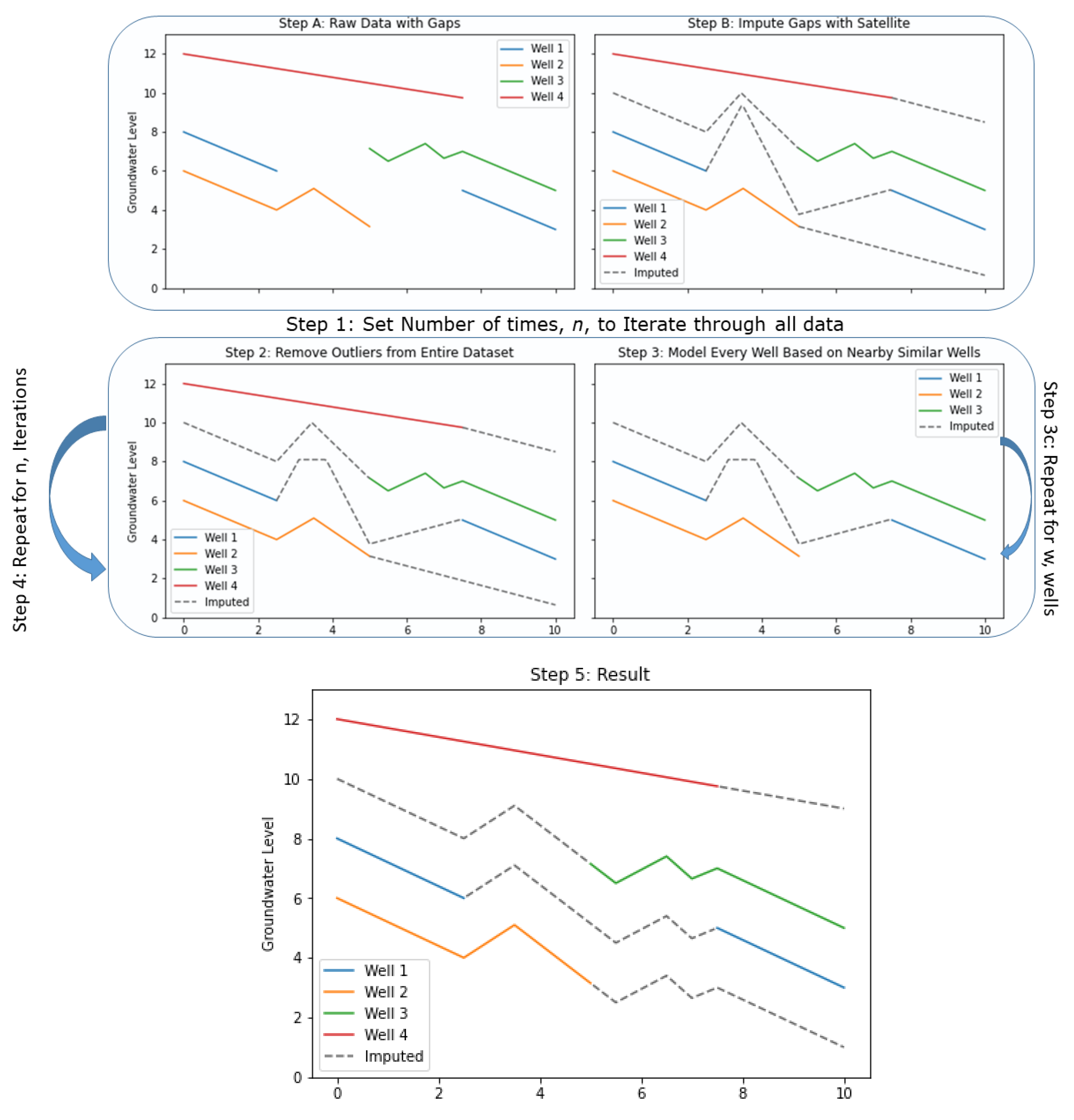
2.1. Methods Overview

We began by generating a complete dataset using independent imputation models for each well; then, we improved our initial predictions by using the spatial correlation among the wells. We provide a high-level overview of the imputation process in Figure 1. Steps A and B can use any method; however, for this paper, we used the methods described by Ramirez et al. [22].
  • Step A: Obtain the raw groundwater data with gaps and preprocess each dataset so that the datasets at each well have the same time steps.
  • Step B: Perform an initial imputation to generate a complete time series dataset for each well. This means that every discretized time step will have an associated value. After imputation, replace any imputed value that has an observed measurement with the original data. The imputation step only fills gaps (i.e., imputation).
Once the initial imputation has been performed and each well has a value, either measured or estimated, the IRM method uses the following steps:
  • Step 1: Select the number of iterations, n, to pass through the entire data set.
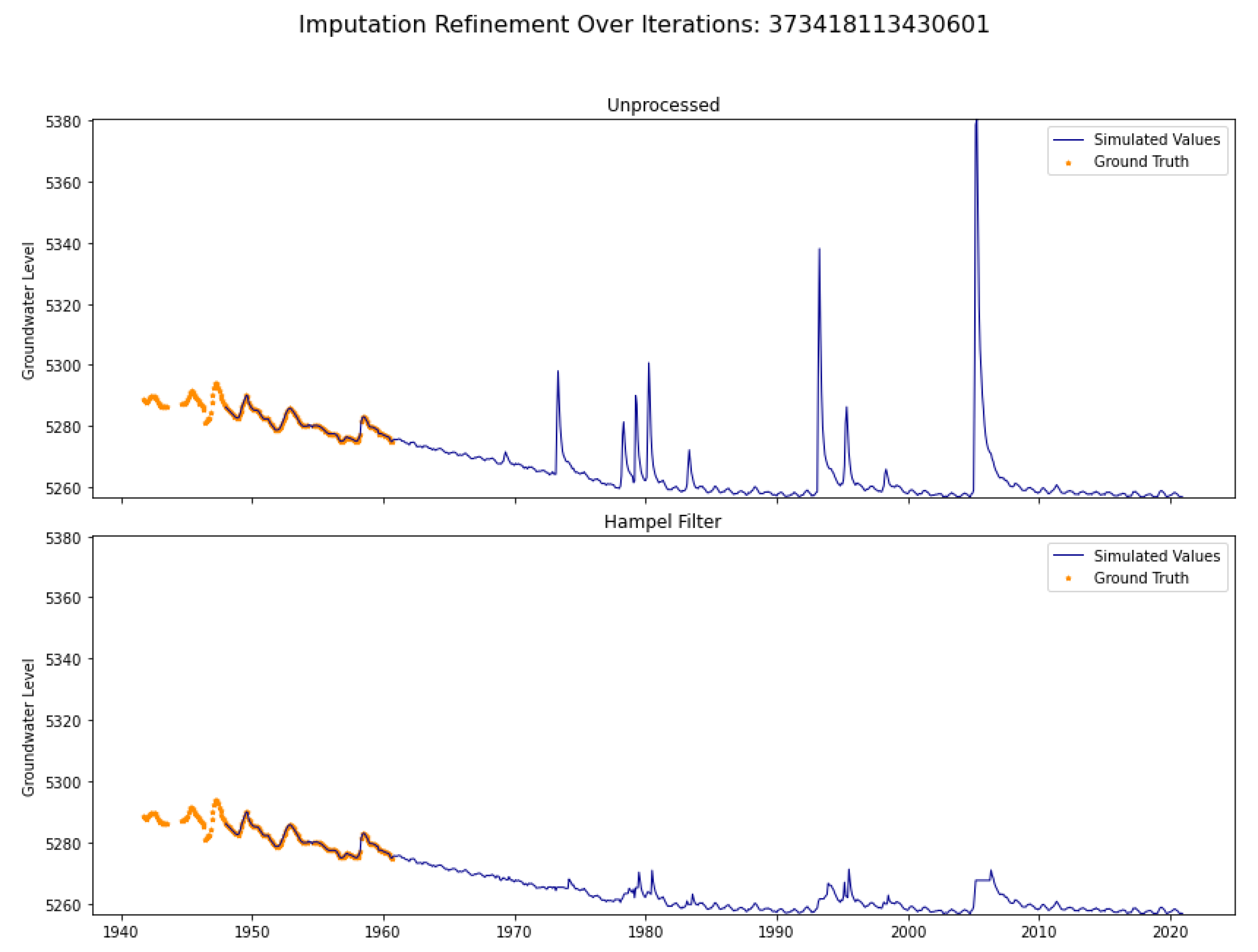
  • Step 2: Use a Hampel filter, described in Section 2.2, to smooth synthetic data spikes or model predictions that are unrealistic for groundwater data. This process removes outliers from the initially imputed dataset. Before each iteration step, apply this filter to remove outliers. The Hampel filter is used so that any anomalies do not propagate errors.
  • Step 3: Iterate through each well, w, in the aquifer. For each well:
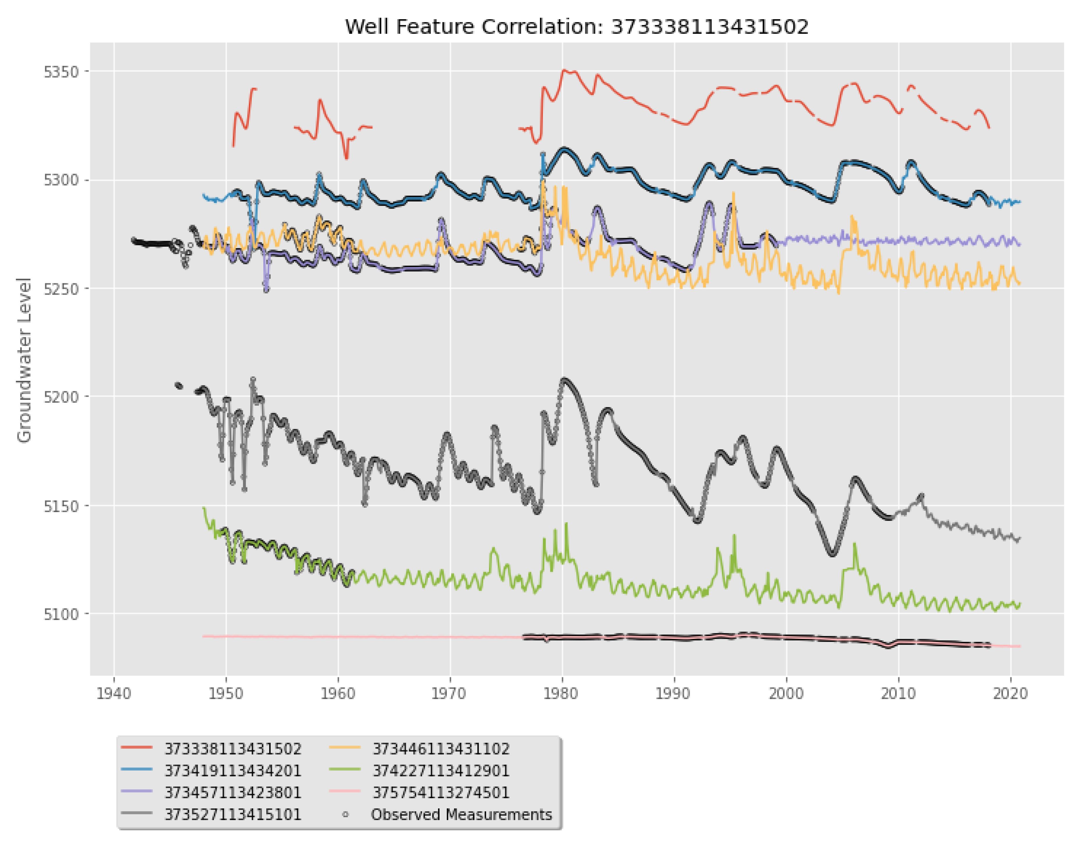
    Step 3a: Select a small set of imputed time series datasets from the wells correlated to the target well. We selected wells based on linear correlation and spatial distance; both ideas are explained in Section 2.3.
    Step 3b: Develop a model for the target well using the time series data selected in Step 3a.
    Step 3c: Run the target well model to generate a complete time series. Replace any predictions that have an observed value with the in situ measurement. The results of every model are updated synchronously at the end of the iteration. This means that an updated representation will not be available as a feature until the next iteration; if a particular well is selected multiple times as a feature, each model will see the same version of the data. Once every well has been visited, the model output is used as the input for the next iteration.
  • Step 4: Repeat Steps 2 and 3 for n iterations.
  • Step 5: Examine the results.

2.2. Hampel Filter

One issue that arises during well data imputation is the effect of extreme data on model predictions over large gaps resulting in outliers [22]. We define outliers as anomalous data points that exhibit large, unphysical changes over short periods and do not follow the general long-term trend of the data. Anomalies occur in time periods where no observed data exist. We know the data are unlikely to be representative of reality because, for example, data will have changes to tens to hundreds of feet in groundwater levels within a few months. If these anomalous data are used in the IRM process to refine groundwater predictions at neighboring wells, the method propagates these anomalous trends to other wells. It is important to eliminate these identified outliers before attempting iterative refinement.
The reason these anomalies occur is that imputed values are based on a regression of meteorological and other data. If the number of observations is minimal, correlations might be extrapolated to scenarios that are not present in the training data, leading to abnormal predictions. This is because the results may overstate a correlation due to the lack of sufficient representative data. Despite this, knowing that an event occurs at a particular time step holds some significance, even if the magnitude of the event is incorrect. Consequently, we substituted these anomalies with more rational values, reducing the frequency of outliers at the start of each iteration.
We used a Hampel filter to detect and remove outliers [30,31,32]. The Hampel filter is a kernel function that is applied to a sequence of size, n (x1, x2, …, xn). The algorithm uses a centered rolling window of size, k, to calculate the local median (Equation (1)). The local median represents the trend at a particular point. Using the local median, the filter calculates the median absolute deviation (MAD), σ ^ M A D , by calculating the deviation of each observation in the window from the local median (Equation (2)) [33]. We set a threshold, T, to represent the maximum allowable deviation from the local median for an observation; we used 3 ∗ σ ^ M A D for T (Equation (3)). Finally, the filter checks if the deviation from the median for the center point of the window is greater than the threshold; if the deviation is larger than the threshold, the point is replaced by the local median, and if the deviation is within the threshold, the value remains unchanged (Equation (4)).
L o c a l   M e d i a n = median y i k 2     i + k 2
σ ^ M A D = 1.4826   Y i L o c a l   m e d i a n
T = 3 σ ^ M A D
y i = L o c a l   M e d i a n y i   , y i L o c a l   M e d i a n > T   , y i L o c a l   M e d i a n T
To apply the Hampel filter, we used a window size of 36 months. We did not replace in situ observations with Hampel-filter smoothed values, even if the in situ value was greater than the allowed deviation. The Hampel filter smooths predicted outliers, preserving local excursions by limiting their size. This allows local excursions to represent local trends that may exist in the data, which is important for Imputation Case III (presented later).
Figure 2 shows an example of applying the Hampel filter; the orange dots are measured values, while the blue line represents imputed values. In the top panel, there are un-realistic large positive excursions in the imputed data occurring in the mid-1970s, around the 1980s, the mid-1990s, and the mid-2000s. We know these excursions are outliers because groundwater levels change slowly, and an increase of 120 feet over 6 months is physically impossible. After the Hampel filter is applied, these excursions remain as local extrema but appear more reasonable, as shown in the bottom panel.

2.3. Well Modeling

We trained a model for each well using the same model architecture; a multi-layer perceptron (MLP) model with two hidden layers of widths of 50 and 100 nodes for the 1st and 2nd layers, respectively. We used L2 regularization to reduce the effects of irrelevant features and 20% dropout between the layers to prevent over-fitting [34]. We optimized our model with ADAM: a commonly used adaptive optimization algorithm that works by calculating the first and second moments of the gradients and also controls the learning rate [34]. For each model, we trained on the measured data at the target well using 19–25 features. The model features consist of 5–11 well features, 1 prior feature, and 13 temporal features.
For any given well, we had limited target data; this meant that it WAS impractical to use an 80–20 testing/training split to estimate errors. To address this lack of data, we used a K-fold cross-validation with 5 folds [35]. K-fold cross-validation works by splitting the data into five groups, each containing a similar number of sequential observations, with 1/5 of the data reserved for testing in each fold. Each fold is sequentially used for testing, with the remaining folds used for training and validation. We computed the error metrics for each fold, then averaged over each of the 5 folds to obtain our overall error metrics.
We utilized the average number of epochs for each fold determined through K-fold validation to train a final model on all the available data. This method enabled us to leverage all the available data for training while still comprehending our error metrics and appropriately selecting the model parameters. We implemented the models using the Python programing language with the TensorFlow package [36,37].

2.3.1. Well Feature Selection

For each well in the IRM method, we selected a subset of neighboring wells from the input dataset to use as model features for training. These wells can be from the initial satellite imputation in the first iterative step or a previous iteration in subsequent steps. The objective of selecting the feature wells was to identify wells that were correlated to the target well. This allowed our IRM model to refine the accuracy of imputation for the target well based on spatial correlations within an aquifer.
We started the feature selection process by computing a correlation metric we call R w 2 between the target well and every feature well in the aquifer. We define R w 2 as a combination of the Pearson correlation coefficient ( r 2 ) and the normalized physical distance (d) between the target well and the feature well using a correlation weight ( w c ) as shown in Equation (5). We used R w 2 to identify wells that exhibited similar usage patterns, mostly represented by the data correlation ( r 2 ), and that experience similar environments such as local climate, water demand, or any isolated regional events, mostly represented by the physical distance (d), that could affect groundwater availability.
R w 2 = w c r 2 1 w c 1 d
We computed the r 2 value between a potential feature well and the target well using only measured data from the target well (i.e., we only used dates on which the target well had measured data) but used either measured or imputed data on these dates from the feature wells. We computed d using the Euclidean distance, x 2 + y 2 where x and y represented the distances in cartesian space, normalized by the largest distance from the target well to any well in the aquifer. This provided d with a value between 0 and 1. We weighed the two similarity measures by the correlation weight, w c , which weighed the importance of both the linear correlation and physical distance when selecting wells as model features.
Through empirical testing, we found that a reasonable range for w c was between 0.90 and 0.95 for small aquifers and 0.70–0.80 for large aquifers. This meant that the distance from the target well to the feature well weighed higher in larger aquifers, as the potential distances were larger. When the aquifer was small, the physical distance between the wells was not as significant, as all wells are generally close, and more distant wells may behave similarly to the target well; therefore, a high linear correlation was more important for the model.
We would expect that the most representative wells are relatively close in the distance because they experience a similar environment. For example, though the measured data at the target well may have some correlation with imputed/measured data at a feature well in an aquifer, if they are separated by hundreds of miles, they might not have the same environment and act differently during periods where data are missing.
However, physical distance alone is not always representative of a similar environment. For example, if there are large variations in elevation over short distances, one well could be driven by snowmelt infiltration while the other is not, or one well could be composed of well-graded gravel while the other is composed of silts and clays. Additionally, wells located side-by-side may be used for different purposes, such as municipal water or agricultural irrigation. Though the environment would be similar, these wells would be pumped on different schedules and exhibit different drawdowns. Thus, nearby wells may not be highly correlated. In the case of a well that is used for municipal water, a more distant municipal well may be more highly correlated than nearby agricultural wells, which exhibit seasonal trends with heavy pumping in the spring and summer. Adjusting w c changes the weight given to the local environment or the weight given to correlated measurements.
During development, we analyzed how many wells should be selected to create the target well model. Initially, we tested using all the wells in the aquifer, but due to various issues, including scalability, computational complexity, and the fact that not all wells in an aquifer are strongly correlated, we found that better results were obtained if we selected only a few, representative wells to use as model features. After some trial and error, we determined a viable procedure. First, we selected the best five wells based on R w 2 ; then, we computed the average R w 2 of these five feature wells, R ¯ w 2 ; next, using this average R ¯ w 2 ,   we determined if additional feature wells should be added. We found that with a high R ¯ w 2 , the initial five feature wells were typically enough to develop a good imputation model, and additionally, less correlated wells typically increased noise in the model, producing less accurate results. However, if the R ¯ w 2 value was low, we could obtain better results if we added additional features to the model. We recommend that if R ¯ w 2 is below 0.60, an additional feature well should be added for every 0.10 below the 0.60 threshold, as summarized in Table 1.
Figure 3 shows the feature selection process for a random target well (shown in red) and the feature wells in multiple colors. The plot shows the time periods where the target well has measured data, with gaps in periods without data. The data in the feature wells used to compute the correlation metric include both measured and imputed data. Notice that the red data (target well) exhibit data gaps, while all the potential feature wells have a complete time series dataset with small circles indicating measured values and lines indicating imputed values. In this case, the R ¯ w 2 was below the 0.6 threshold, so we added a 6th feature well.
As shown in Figure 3, a lower R ¯ w 2 does not necessarily mean that the available feature data are poor. Both the target well and the blue, gray, and purple feature wells share groundwater levels that increase between 1978 and 1980. The blue and gray wells have an almost complete measured data set, with only a few periods of imputed values; these values closely follow the trends in the target well. Both of these wells have significant amounts of measured data, with limited imputed data, so we expected that these two feature wells would provide a more accurate imputation model for the red well. The yellow well was visually correlated with the target well but had less measured data and more imputed data. However, this could still be informative because many of the peaks seemed to match. The other available feature wells appeared to be less correlated, which resulted in the low R ¯ w 2 .

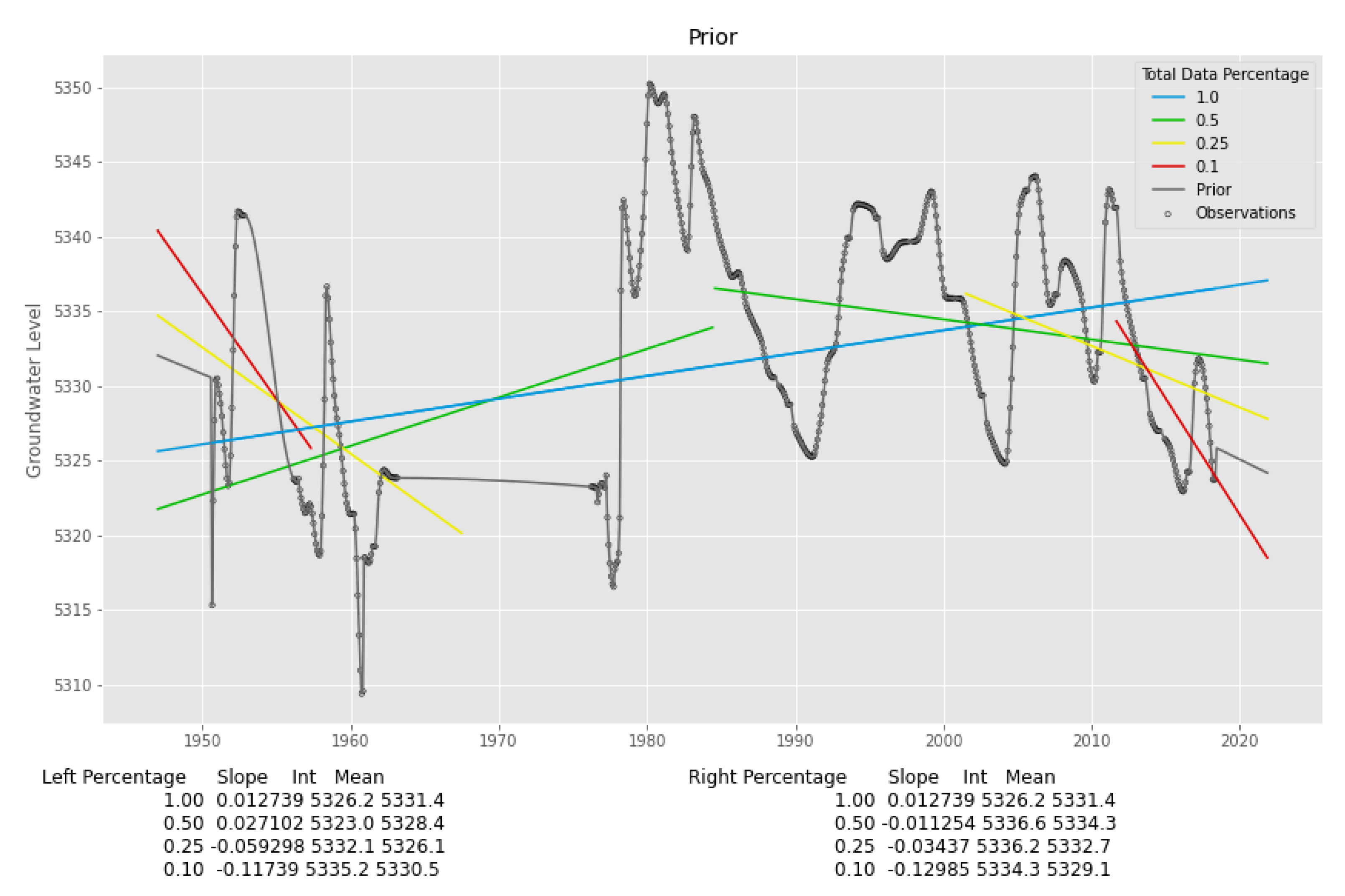
2.3.2. Prior Features

Similar to Ramirez et al. [22], we generated a prior based on trend estimates computed using a data-centric prior algorithm. To develop the data-centric prior, we interpolated within the temporal data range using a piecewise cubic Hermite interpolating polynomial (PCHIP) interpolation [21]. PCHIP honors data limits and does not generate data outside the existing values. Next, we linearly extrapolated outside of the temporal data range to the extent of the imputation window to complete the prior estimate of the well data. We performed the extrapolation in two parts, as shown in Figure 4. First, we calculated four linear regressions for each side of the data using 10%, 25%, 50%, and 100% of the data. We prepared the data for least-squares regression by removing outliers greater than three standard deviations from the subset of data. This was performed to obtain the general direction of the data. In Figure 4, these estimates are shown as red, yellow, green, and blue lines for the trends based on 10%, 25%, 50%, and 100% of the data on each side, respectively. We build our linearly extrapolated trend by averaging the slopes of these four linear regressions as the average slope and the mean of the 10% data partition as the y-intercept to extrapolate the imputation limits on each side. We limited the extrapolated data to six standard deviations above or below the mean of all observations. We added this limit for situations where either the average slope used for extrapolation was large, or the extrapolation period was long, and the extrapolation resulted in unrealistic values. We then combined the interpolated data with the extrapolated data to generate a prior estimate of the well data.
Figure 4 shows the prior as a gray line for an example well. In summary, we used PCHIP interpolation within the limits of the data, then extrapolated these to the limits of the study period: from July 1945 to June 2023. It can be noticed that the gray line follows regions with existing data closely, generates smooth curves over data gaps (e.g., 1955–1958), and extrapolates a weighted average trend outside the limits of the data (e.g., <1950 or >2018).
Ramirez et al. [22] generated multiple prior features from the prior estimate to use as model features in varying window sizes. For the IRM model, we only generated one prior feature using a 24-month centered moving window to smooth the initial prior. Figure 5 shows this prior use as a model feature for the same well shown in Figure 4. We found that a window size of 24 months provided enough context on the structure of the data without overpowering relationships in the well features. Figure 5 shows that this prior feature does not exactly match the measured data but instead encodes the general trends. However, this prior constrains the model to rely on selected feature wells to fit the data rather than relying on the inductive bias from the prior generated by the researchers.

2.3.3. Temporal Features

We used thirteen temporal features to analyze the time series data in every model. Twelve of these features were created using one-hot-encoding, which is a technique that converts categorical variables, such as the months of the year, into multiple binary features. Each feature represents a single category, such as January or February, and has a value of 1 or 0. One-hot-encoding is useful because there is no inherent order or ranking in the categories, and it allows the model to understand the unique characteristics and patterns related to each month without assuming any ordinal relationship between them. This can improve the model’s ability to make accurate predictions, especially for data with seasonality [35] (Table 2).
We created the thirteenth feature using sequential encoding, which assigned a unique integer value to each observation, such as 0, 1, 2, 3, etc. [35]. This method is useful when there is an inherent order or ranking in the data. For example, February 1948 comes after January 1948 and, therefore, should be assigned a larger value insinuating order. Sequential encoding allows the model to understand the ordinal relationship in the data, which is useful for modeling linear trends. Before using the sequential encoding in our model, we normalized the sequence between 0 and 1 and called that value “Decimal Time”. We demonstrate these features in Table 2. By using both one-hot-encoding and sequential encoding as features, our model could better incorporate and make predictions based on the temporal aspect of the data.

2.4. Iterative Refinement

The process of iterative refinement is to take the feature dataset, whether from satellite imputation or a previous iteration, and iteratively model each well in the aquifer. After modeling each well, we used a direct insertion to replace predicted values with the actual in situ values where they were available. By incorporating these observed values into the predictive model, our approach remained anchored to empirical observations, thereby avoiding overfitting and enabling the method to achieve greater robustness and generalizability. The feature data are updated synchronously at the end of the iteration, meaning new outputs, with new estimates for the missing values, were saved in memory until the end of the iteration, then the feature data were updated all at once, and these updated values became the input for the next iteration. Through each iteration, the feature data became more representative of trends in the aquifer, and as a result, the model outputs at the end of each iterative step were better, generally improving accuracy.
The IRM allowed information from nearby wells to propagate through imputation. This improves accuracy because these different wells may have been measured in situ in time periods where the target well did not have data. As imputed values at the individual wells were improved based on their neighbors, they also improved their neighbors when used as a feature in the next iteration.
We found that two iterations were generally sufficient to obtain good results. The first iteration essentially removed any noise and corrected trends from satellite imputation, and the second iteration strengthened spatial trends that were not captured during the first iterative pass to improve the model accuracy. It is reasonable to assume that using a higher number of iterations would help; however, our experience showed that the improvements, if any, were marginal, sometimes even producing poorer results. Using more iterations can also cause feedback loops where a particular pattern is swapped between a subset of wells for each iteration. Because the resulting signal is changing, this problem is difficult to track when the numbers of wells become large.

3. Results

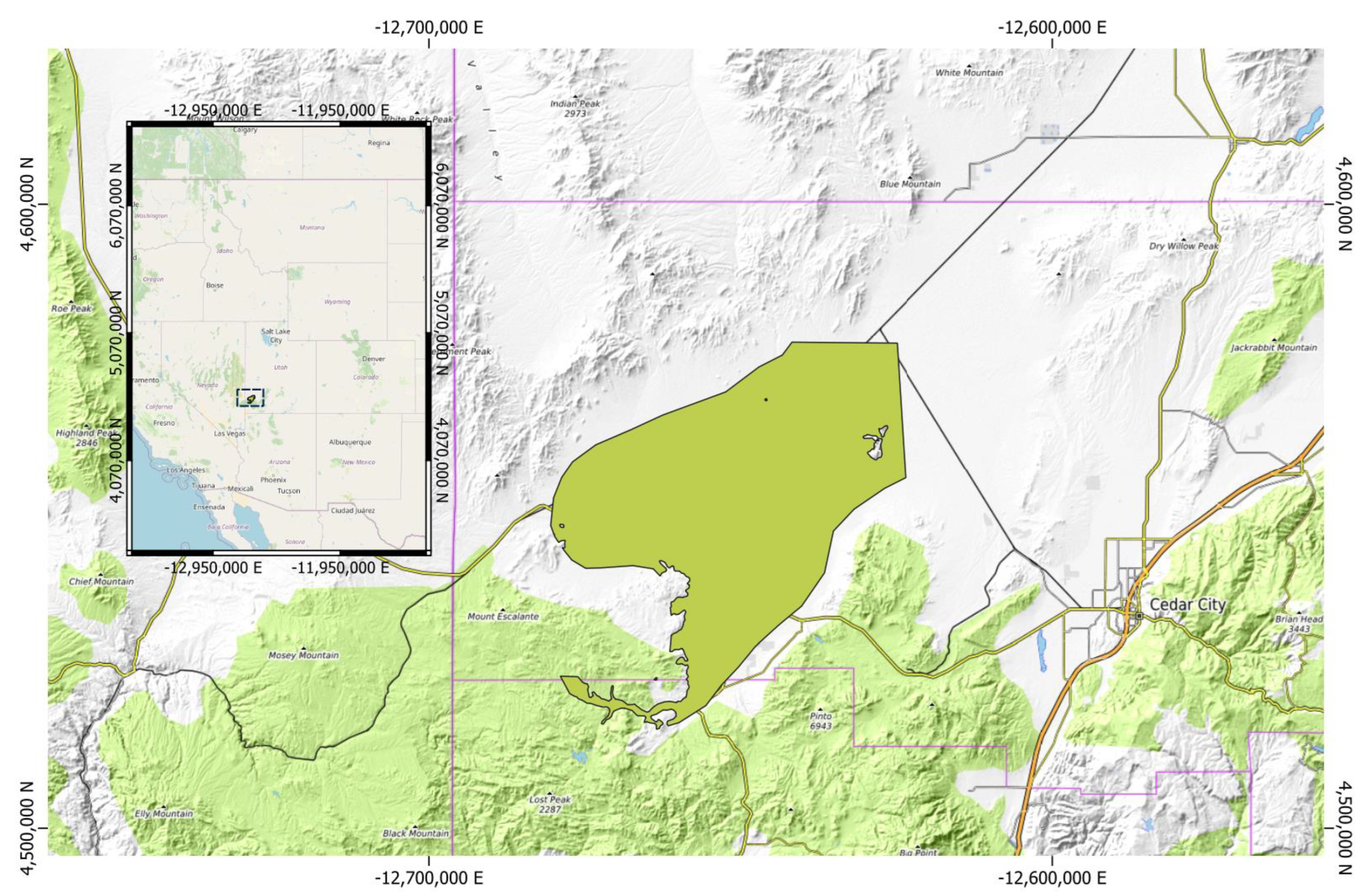
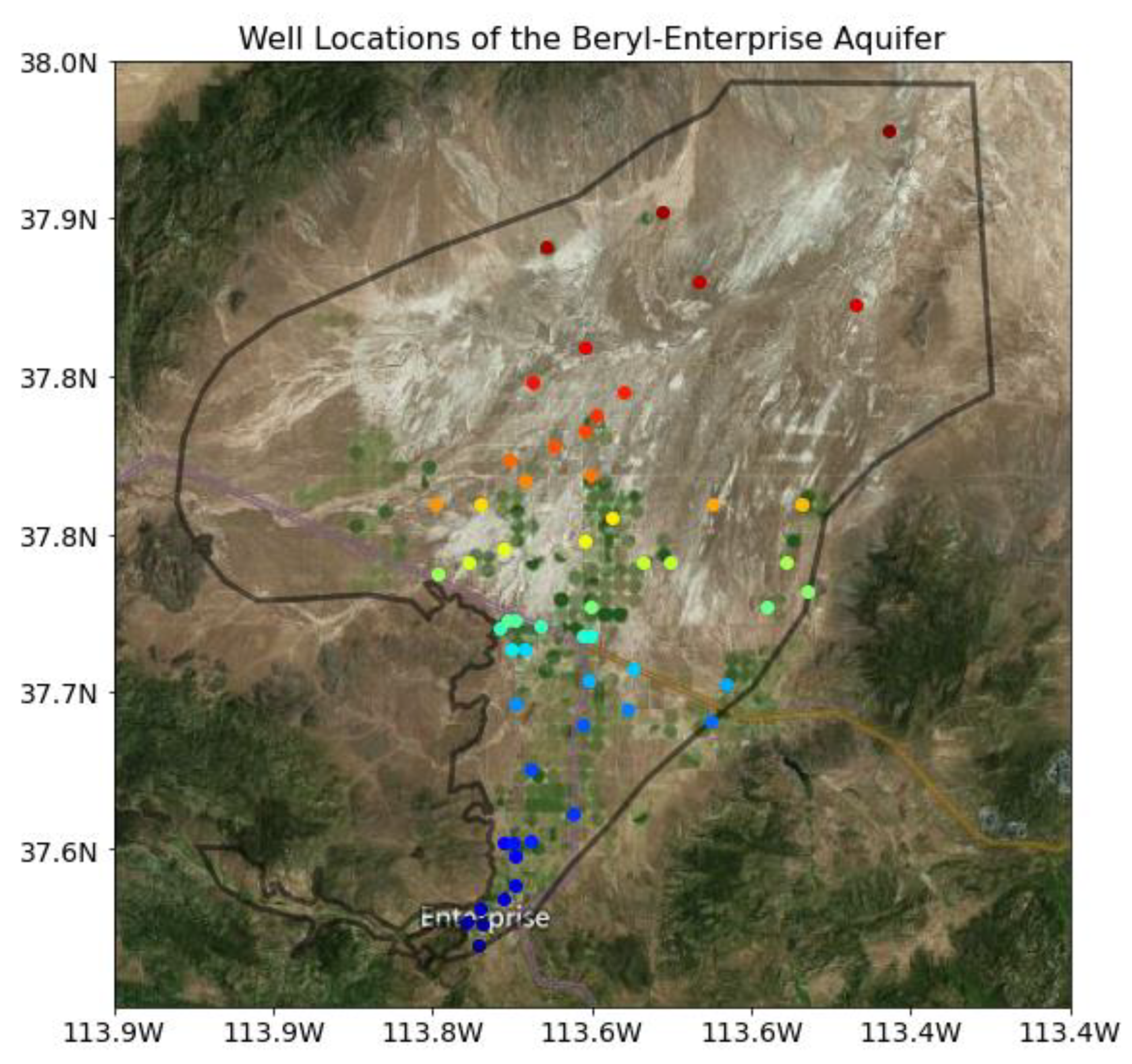
3.1. Case Study: Beryl-Enterprise Utah Aquifer

To demonstrate the IRM method, we used historical groundwater level data from the Beryl-Enterprise aquifer in Utah’s Escalante desert, the same region analyzed by Ramirez et al. [22] and Evans et al. [21]. The Beryl-Enterprise aquifer is part of the Great Basin aquifer located in the Beaver River drainage basin [9]. The aquifer has an area of approximately 433 square miles (1121.4 sq. km) located 40 miles (64.3 km) west of Cedar City, Utah (Figure 6).
We used in situ groundwater level observation data from the National Water Information System (NWIS) published by the United States Geologic Survey (USGS) [38]. Of the 751 possible wells within the geographic boundary of the aquifer, only 57 had at least 50 observations in unique months over the imputation window from January 1948 to December 2020. We selected 50 observations as the minimum for this study, following the recommendations of Ramirez et al. [22].
We prepared the groundwater measurement data for imputation by converting the measurements from depth-to-groundwater to groundwater levels, then removed outlier values that were larger than three standard deviations from the mean of the data. Next, we used PCHIP to resample the groundwater data to the beginning of the month and interpolated the data over small gaps of less than 120 days (4 months). This process generated synchronous observations between the Earth observation data sets and the other wells during iterative refinement [21,22].
Figure 7 shows the locations of the wells in the aquifer boundary. From this figure, we can see that many of the wells are near agricultural irrigation fields (seen as dark to muted green circles in the image) and are most likely used for agricultural irrigation, while another group (red) is not near any agricultural fields and are probably not used for agriculture. Figure 8 shows the data availability for each color-coded well. Figure 9 shows the well data after cleaning and PCHIP interpolation. We identified several long-term trends in the data, with several wells exhibiting a similar downward trend, especially those near agricultural areas. Others were exhibited as more stationarity. We could see several potential groupings, but due to the amount of missing data, the nature of the clusters was not clear. The colors in Figure 7, Figure 8 and Figure 9 are based on the north–south distance of the well in the aquifer and are used to help visualize the data with spatial context.

3.2. Aquifer Results
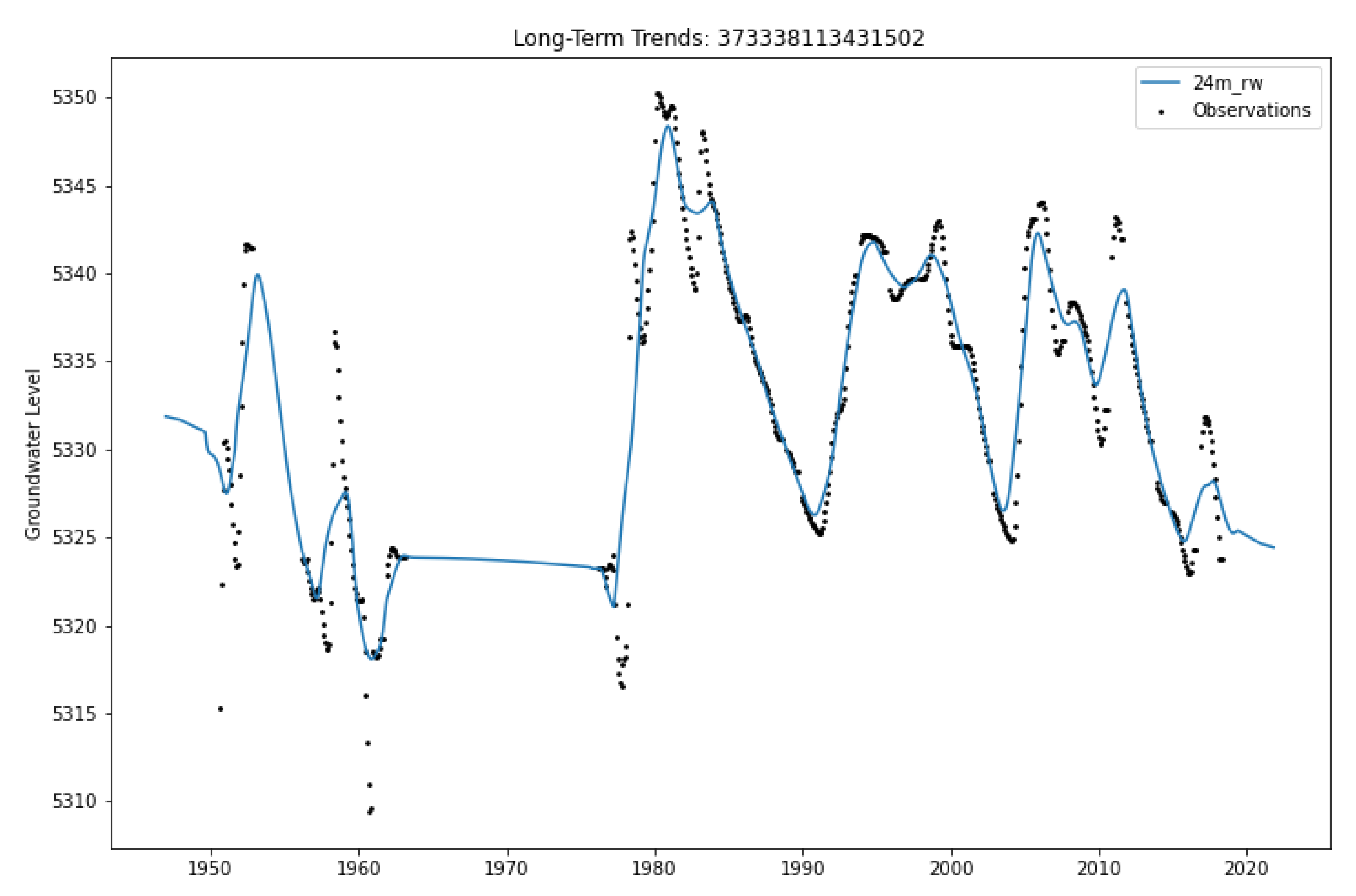
Figure 10 shows the results of the initial satellite imputation in the top right panel and the IRM results from the first to the second iterations in the bottom left and right panels, respectively, for every well in the aquifer. Since many of these wells are used in agriculture, we expected that the agricultural wells would exhibit similar trends because they are close to each other spatially, have similar conditions, and are used for similar purposes. We expected similar groupings for the wells used for either livestock, water supply, or domestic use.
As the imputation process refined the data, the graphs show there are at least three distinct well patterns in this aquifer. The group of five wells with the highest groundwater levels was located at the base of the mountains. These wells do not appear to be used for agricultural purposes based on their location and trends. In the second cluster, the wells are located near the agricultural fields, and the data shows that groundwater levels in these wells dropped up to 150 feet over the imputation window. The final group represents the wells located far from the fields and away from the mountains; they may be used for municipal purposes or single dwellings. These wells have a lower groundwater level but did not exhibit a long-term decline in the group we assigned to agriculture. The difference in elevation between the highest five wells and the remainder of the wells could indicate that there are two aquifers here, though the USGS assigns all these wells to a single aquifer.
We believe that the differences in trends are due to varying pumping patterns, differences in groundwater usage, or, potentially, the wells were completed in different layers of this aquifer. There is a clear change from the satellite imputation results to the IRM results, as the obvious data excursions that occurred in some wells were removed, and the data followed trends and behaviors that we expected from groundwater levels. Figure 10 shows that there are only small changes between the results for iterations 1 and 2.

3.3. Well Details

We selected several wells to evaluate in detail and to demonstrate the strengths along with the various issues and challenges with the IRM method. Well 37345711342801 is a relatively simple imputation as it has significant measured data and few gaps, though the measured data stop prior to 2000 resulted in an over the 20-year gap at the end of the period. The well had 550 monthly observations between January 1948 and March 1999 and 75 observations before the imputation window (Figure 11). The imputation window is marked by the solid lines in the figure and extends from 1948 to 2021. The last 20 years have no measured data. The satellite imputation step results in data that show relatively steady groundwater levels over this 20-year period with some seasonal variation. However, as we refined this initial imputation with the IRM, a trend appeared in the data where groundwater levels generally decreased with rebounds in 2008 and 2011. Figure 10 shows that this is a common feature among several wells and probably represents better imputation results. An interesting observation is that the periods of rebounds are present as anomalies in the satellite imputation, though their shape and magnitude are very different. The IRM shows an increase in RMSE and a decrease in r2 compared to satellite imputation. This is due to one-fold being poorly modeled and influencing the average metrics. However, the IRM results are qualitatively better, based on a visual comparison to the results data from other wells in the aquifer. The results of the IRM iterations follow the general trends in the aquifer more closely.
Figure 12 shows the results for Well 374504113370201, which had 135 unique monthly observations between 1950 and 1963. This well had no data after 1963, which leaves a 57-year gap. In contrast to the previous well, this situation relies more on the prior estimates of groundwater to provide trends and structure for the satellite imputation. The measured data show a seasonal periodicity with a significant decreasing trend. The satellite imputation results demonstrate a long-term decreasing trend until the imputed results reached the limit placed on the prior features around 1972, after which the curve then flattens. The results of satellite imputation contain large anomalies between 1993 and 2008. After applying the IRM, we could see the downward trend continuing with exceeding limits placed on the prior features used in the satellite imputation model. This is an instance where the priors used as features were incorrect, but the IRM improved the imputation based on its correlation with other wells in the aquifer. When compared to other wells in the aquifer with more observations (Figure 10), the trend computed by the IRM is more valid. There is a significant difference in the range of groundwater levels between the satellite imputation (5090–5135 ft) method and iterative refinement (5050–5135 ft). The satellite imputation model assumed that the prior estimate could not exceed about 85 feet. The final IRM results appear more reasonable than the satellite imputation results and follow other wells in the aquifer well. However, it would be impractical to not restrict the priors used in the satellite model, as large changes are usually the result of anomalies. In this situation, the RMSE and r2 values were improved considerably by IRM. This well demonstrated the power of adding the IRM method to the satellite imputation.
Well 373446113431102, as shown in Figure 13, had 110 observations; 79 occurred between April 1955 and October 1961, with 31 observations between April 1976 and October 1978. The measured data do not provide much information on either long-term trends or seasonality. This is an extremely difficult imputation situation; nevertheless, the satellite imputation created a reasonable imputation given such sparse data. However, the satellite imputation created several excursions that were unreasonably high. The IRM-identified correlated wells were able to build a model that generated reasonable imputation results. While the RMSE and r2 values decreased, after two iterations, the general structure shown in other feature wells was transferred to this well, which was impressive given that such little context from any measured data was available. This well-illustrated the benefit of the iterative refinement approach, as some wells have too few examples to build an independent model. Yet, when the patterns in these wells were observed at other locations, we could transfer the data structure.

3.4. Validation through Water Storage Analysis

Ramirez et al. [22] showed that imputation results could be difficult to evaluate because the training and testing error metrics alone do not necessarily represent how well the imputed signal corresponds to the true signal. It is difficult to find wells with complete data sets where some data could be reserved for ground truth. To validate our results and methods, we compared aquifer storage values computed using the IRM imputation results with the values from Mower and Sandberg [9], who concluded that between 1937 and 1978, the aquifer lost approximately 1.60 km3 (1.3 million acre-feet) of storage. This value was derived based on a storage coefficient of 0.2.
To compare our imputation results with these published values, we performed a geospatial interpolation of the imputed well values in the aquifer at each time step, then used the differences between the water surface level maps to understand how storage has changed over time. We used kriging interpolation to build a surface of the aquifer every month between 1948 and 2020 (Figure 14). We used a model variogram with a nugget of 0 and a range of 25% for the maximum length of the aquifer; we set the variogram sill to the variance of the data for any given month. Once we generated these surfaces, we calculated monthly groundwater storage changes by subtracting the current surface from the previous month’s surface and multiplying the volume by a storage coefficient of 0.2 [9,21]. We then cumulatively summed these changes to generate a cumulative storage depletion curve (Figure 15).
The results from the IRM method estimate that groundwater storage was reduced by approximately 1.21 million acre-feet between 1948 and 1978. Over the 70-year window, the aquifer lost over 2.87 million acre-feet of storage (1.49 km3) (Figure 15). Our results indicate that the aquifer experienced a steady decline in storage over time, with the rate of depletion increasing in recent years. This is consistent with the results of previous studies and highlights the need for sustainable management practices to ensure the long-term productivity and health of the aquifer [39,40]. Overall, our geospatial analysis and imputation methods provide a valuable tool for understanding and monitoring the changes in groundwater storage over time. These results could be used to inform water management decisions and aid in the development of strategies to conserve and protect this vital resource.

4. Discussion

When applying the IRM, there are three general cases that occur that can have significant effects on the accuracy of the imputation results and our confidence in the imputation (Table 3). In this section, we describe the following three general cases from easy to difficult in detail.
It is critical to remember that, as with most regression approaches, the results are only as good as the data used. Generally, if the initial imputation results are poor, iterative refinement acts as a negative feedback loop, and results may diverge. Nevertheless, when the input dataset is close to the real values, data are clean, and when good priors have been made, iterative refinement is able to obtain good results as it uses measured data from other wells in addition to good prior estimates to help impute gaps in the target well.

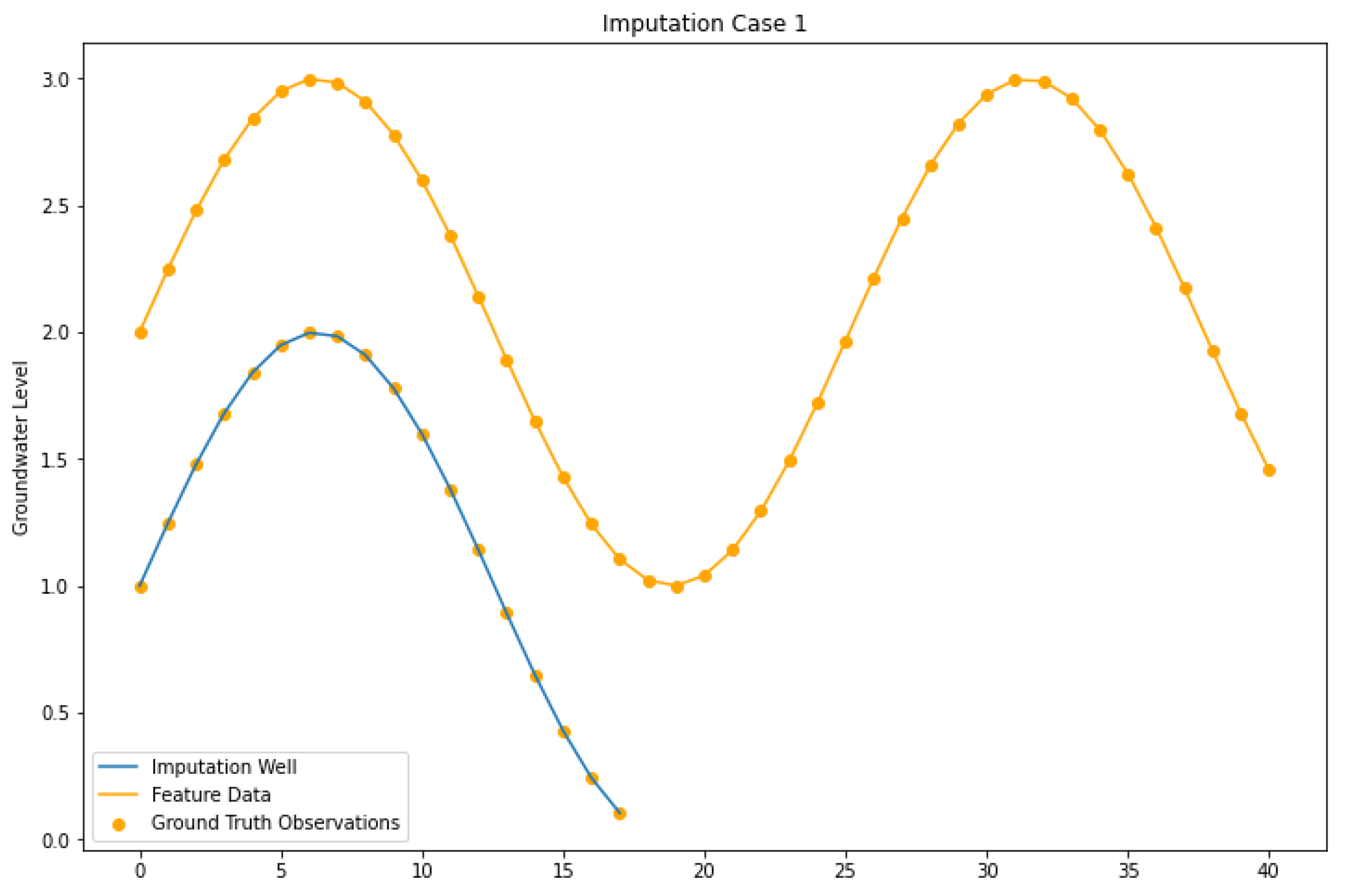
4.1. Imputation Case I

Imputation Case I is the best-case scenario for iterative refinement. This is when we input a target well using a feature well that has a complete, measured dataset, and the feature well is correlated with the target well in regions where they both have data. Figure 16 presents this example; both the target well (blue) and the feature well (yellow) are correlated over the period when they both have measurements (left side of the figure). Ideally, the feature well will have only a few imputed values and mostly measured values. In this situation, we can have confidence that if these wells respond similarly to environmental conditions, refinement will produce good results because the signal of the feature well can be transferred to the target well. Using multiple feature wells that depict similar patterns based on ground truth data increases our confidence that our imputation will be accurate.

4.2. Imputation Case II

Imputation Case II is when the imputation well shows similar trends to the feature well, either based on measured observations or imputed values, but the feature well contains noise in part of the overlapping time range (Figure 17). These are the situations that benefit most from the IRM approach. This situation is common, as when monitoring at a well stops, monitoring at a nearby well used for a similar purpose often begins.
This situation is challenging because we need sufficient information to know that the wells are correlated so that they can be selected as features, even though there is little evidence to base it on. Depending on how much noise and measured data are available in the overlapping time range, the feature well may not be selected to model the target well. Additionally, if too much noise exists in the training data, the important trends or features may not be transferred, only the noise. However, if the correlation with the feature well is identified, selected, and characterized during training, we can expect the imputation to provide good results as they are based on measured data in the area where the target well has no data.
Generally, if the wells have sufficient information to show that they are correlated, they will be part of a positive feedback loop where the feature well supports the target well, and the target well becomes a strong feature well when they swap roles. The key is to identify and select wells that are correlated enough for our assumptions to be valid. Having a strong initial imputation with a good prior, as is conducted in the satellite imputation method [22], is crucial as this provides good estimates of how groundwater levels have changed based on historical meteorological events and support identifying wells that are correlated. Though the satellite imputation is imperfect, it produces independent results that are good enough for iterative refinement to work.

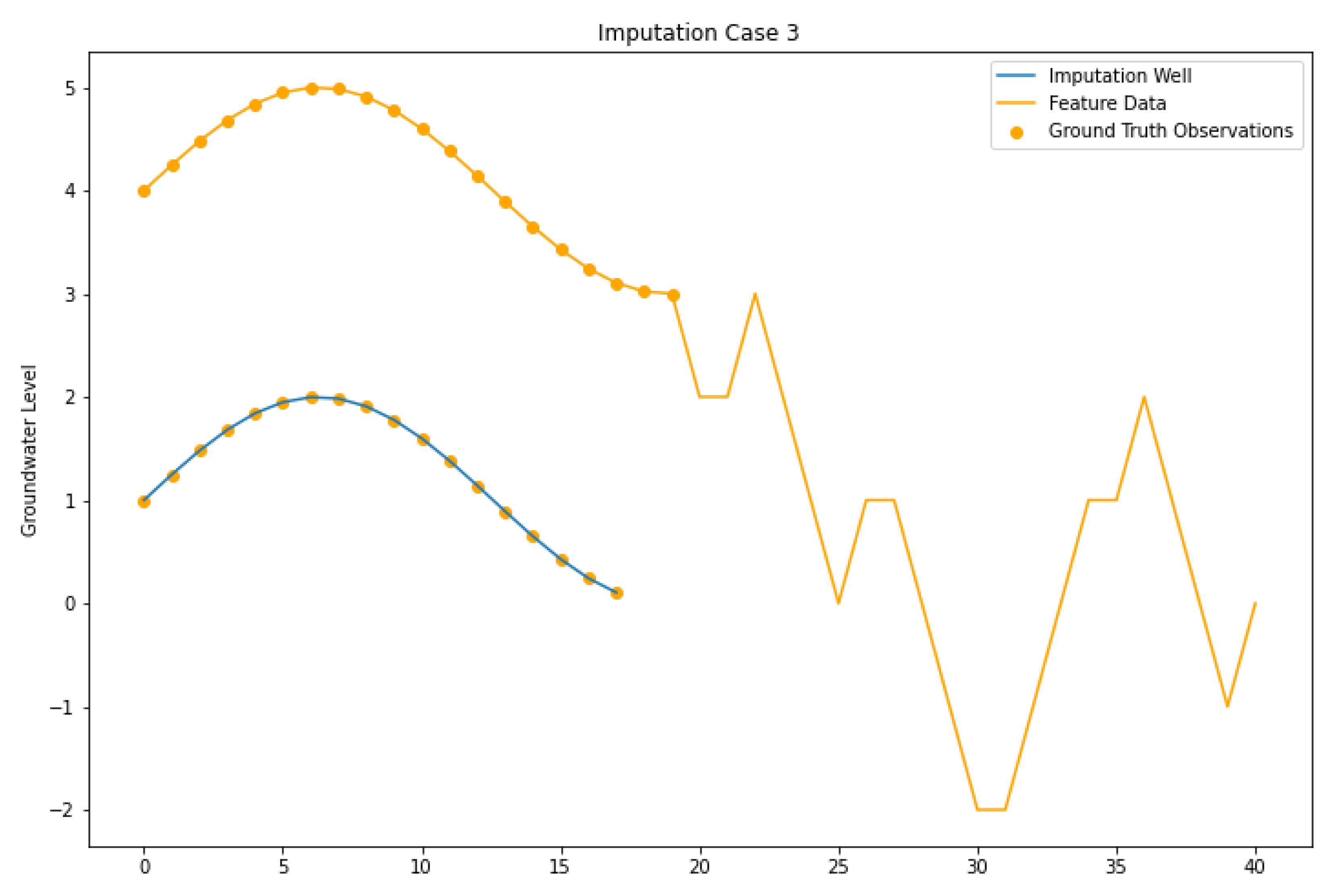
4.3. Imputation Case III

Imputation Case III is when the feature well and the imputation well only have measured values in their overlapping time range (Figure 18). This is the most difficult case to obtain reliable results from and, unfortunately, is common due to limited aquifer monitoring. IRM, similar to any machine learning algorithm, generally clings heavily to this feature during training as there exist strong similarities. However, the predictions may be inaccurate as the inputs used for prediction are noisy variations of the independent features on which the model was built. Depending on the amount of noise, the prediction inputs may not represent the same signals that the model was trained on. In other words, the model uses a guess to estimate a value.
When this situation arises, having multiple representative wells may provide the context needed to obtain the best results. We have observed that if multiple feature wells are classified as Case III through iterative refinement, their imputation results converge to a similar trend. However, it is difficult to evaluate the quality of the imputation as there is little measured data with which to qualitatively compare. There are edge cases of this situation where all feature data used in imputation only share measured data with the imputation well during the training period. In this case, there is no new information, so the IRM either does not improve the previous estimates or could become caught in a negative feedback loop with different results.

5. Conclusions

Obtaining and managing groundwater data is difficult—especially data for longer time periods. To solve the problem of missing historical observations, we developed the IRM data imputation refinement approach for the use of spatial correlations that could improve data imputation. IRM works on any complete dataset that is a mixture of measured and imputed values and refines the imputed values. The IRM method demonstrated accurate results for the Beryl-Enterprise aquifer in Utah, where many wells were missing large periods of observations. Though we only showed IRM when applied to Beryl-Enterprise, it can be used globally if sufficient groundwater observations exist. For our demonstration, we used the method outlined in Ramirez et al. [22] for the initial imputation, but any other method could also be used. Once the imputed data are refined, and the aquifer has a complete data set, many analysis applications are possible; researchers can use these data to understand climate change, population growth, or critical societal events affecting aquifer storage. These data could also be used to make preliminary plans for infrastructure development.
This method allowed us to refine imputation results based on spatial correlation. This is based on the idea that wells in the same aquifer experiencing a similar environment (i.e., climate and pumping patterns) exhibit similar changes. If wells have a similar environment, meaning they exhibit similar patterns and have similar usage, we can assume that the wells exhibit similar responses. Though a single well often does not have a complete dataset, several wells contain measured data that provide partial information to characterize well behavior. Using IRM in conjunction with satellite-based imputation provides valuable insights into aquifer behavior, even when limited or no data are available at individual wells.
This method revealed patterns and trends in an active desert environment aquifer and revealed the stresses of agriculture and long-term drying on the aquifer. The details present in this data analysis revealed the possibility of two overlapping aquifers not previously recognized. Future analyses using this method have the potential to reveal more details about aquifers in regions around the world.

Author Contributions

Conceptualization, G.P.W. and N.L.J.; methodology, S.G.R. and G.P.W.; software, S.G.R.; investigation, S.G.R., G.P.W. and N.L.J.; data curation, S.G.R.; writing—original draft preparation, S.G.R. and G.P.W.; writing—review and editing, S.G.R., G.P.W., D.P.A., J.R. and N.L.J.; supervision, G.P.W. and N.L.J.; project administration, N.L.J.; funding acquisition, N.L.J. and G.P.W. All authors have read and agreed to the published version of the manuscript.

Funding

This work was supported by the National Aeronautics and Space Administration ROSES SERVIR Applied Research Grant 80NSSC20K0155 and from USAID under the SERVIR-West Africa hub. Some author contributions were supported under NOAA Grant NA22NWS4320003 Cooperative Institute for Research to Operational Hydroinformatics (CIROH).

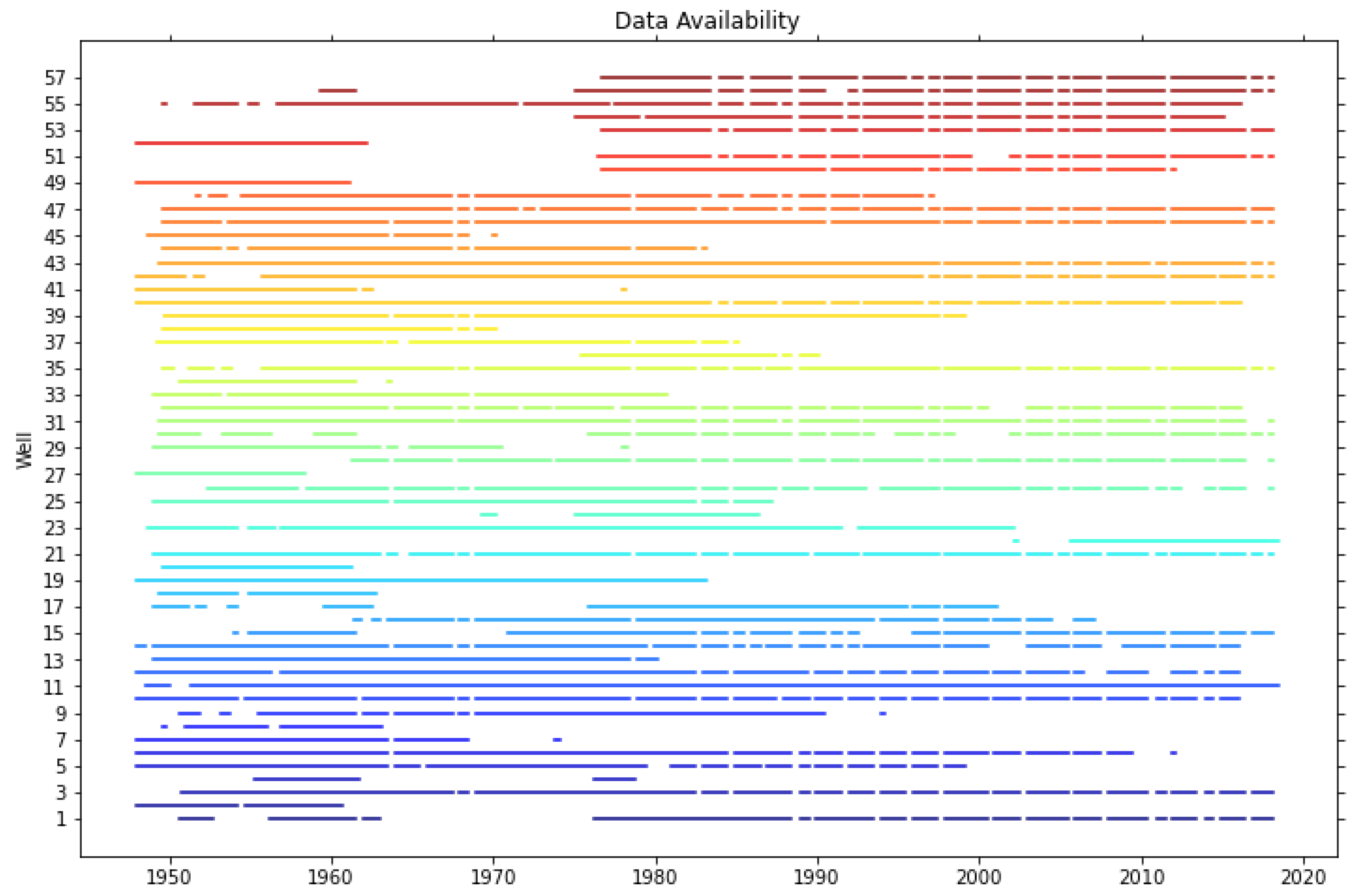
Data Availability Statement

Not applicable.

Acknowledgments

We would like to acknowledge Michael Stevens who worked as part of the Hydroinformatics Laboratory and was instrumental in developing the imputation notebook that accompanies this article.

Conflicts of Interest

The authors declare no conflict of interest.

References

  1. Barber, N.L. Summary of Estimated Water Use in the United States in 2005; U.S. Geological Survey: Reston, VA, USA, 2009.
  2. Giordano, M.; Villholth, K.G. The Agricultural Groundwater Revolution: Opportunities and Threats to Development; CABI: Long Beach, CA, USA, 2007; ISBN 978-1-84593-173-5. [Google Scholar]
  3. Konikow, L.F.; Kendy, E. Groundwater Depletion: A Global Problem. Hydrogeol. J. 2005, 13, 317–320. [Google Scholar] [CrossRef]
  4. Sophocleous, M. Interactions between Groundwater and Surface Water: The State of the Science. Hydrogeol. J. 2002, 10, 52–67. [Google Scholar] [CrossRef]
  5. Fogg, G.E.; LaBolle, E.M. Motivation of Synthesis, with an Example on Groundwater Quality Sustainability. Water Resour. Res. 2006, 42, W03S05. [Google Scholar] [CrossRef]
  6. Famiglietti, J.S. The Global Groundwater Crisis. Nat. Clim Change 2014, 4, 945–948. [Google Scholar] [CrossRef] [Green Version]
  7. Beran, B.; Piasecki, M. Availability and Coverage of Hydrologic Data in the US Geological Survey National Water Information System (NWIS) and US Environmental Protection Agency Storage and Retrieval System (STORET). Earth Sci. Inform. 2008, 1, 119–129. [Google Scholar] [CrossRef] [Green Version]
  8. Barbosa, S.A.; Pulla, S.T.; Williams, G.P.; Jones, N.L.; Mamane, B.; Sanchez, J.L. Evaluating Groundwater Storage Change and Recharge Using GRACE Data: A Case Study of Aquifers in Niger, West Africa. Remote Sens. 2022, 14, 1532. [Google Scholar] [CrossRef]
  9. Mower, R.W.; Sandberg, G.W. Hydrology of the Beryl-Enterprise Area, Escalante Desert, Utah, with Emphasis on Ground Water; with a Section on Surface Water; Technical Publication; Utah Department of Natural Resources, Division of Water Rights: Salt Lake City, UT, USA, 1982; Volume 73, p. 86. [Google Scholar]
  10. Evans, S.W.; Jones, N.L.; Williams, G.P.; Ames, D.P.; Nelson, E.J. Groundwater Level Mapping Tool: An Open Source Web Application for Assessing Groundwater Sustainability. Environ. Model. Softw. 2020, 131, 104782. [Google Scholar] [CrossRef]
  11. Freeze, R.A.; Cherry, J.A. Groundwater; Prentice-Hall: Hoboken, NJ, USA, 1979; ISBN 978-0-13-365312-0. [Google Scholar]
  12. Alley, W.M.; Healy, R.W.; LaBaugh, J.W.; Reilly, T.E. Flow and Storage in Groundwater Systems. Science 2002, 296, 1985–1990. [Google Scholar] [CrossRef] [Green Version]
  13. Becker, M.W. Potential for Satellite Remote Sensing of Ground Water. Groundwater 2006, 44, 306–318. [Google Scholar] [CrossRef]
  14. McStraw, T.C.; Pulla, S.T.; Jones, N.L.; Williams, G.P.; David, C.H.; Nelson, J.E.; Ames, D.P. An Open-Source Web Application for Regional Analysis of GRACE Groundwater Data and Engaging Stakeholders in Groundwater Management. JAWRA J. Am. Water Resour. Assoc. 2021, 58, 1002–1016. [Google Scholar] [CrossRef]
  15. Rodell, M.; Chen, J.; Kato, H.; Famiglietti, J.S.; Nigro, J.; Wilson, C.R. Estimating Groundwater Storage Changes in the Mississippi River Basin (USA) Using GRACE. Hydrogeol. J. 2007, 15, 159–166. [Google Scholar] [CrossRef] [Green Version]
  16. Sun, A.Y. Predicting Groundwater Level Changes Using GRACE Data. Water Resour. Res. 2013, 49, 5900–5912. [Google Scholar] [CrossRef]
  17. Tao, H.; Hameed, M.M.; Marhoon, H.A.; Zounemat-Kermani, M.; Heddam, S.; Kim, S.; Sulaiman, S.O.; Tan, M.L.; Sa’adi, Z.; Mehr, A.D.; et al. Groundwater Level Prediction Using Machine Learning Models: A Comprehensive Review. Neurocomputing 2022, 489, 271–308. [Google Scholar] [CrossRef]
  18. Ahmadi, A.; Olyaei, M.; Heydari, Z.; Emami, M.; Zeynolabedin, A.; Ghomlaghi, A.; Daccache, A.; Fogg, G.E.; Sadegh, M. Groundwater Level Modeling with Machine Learning: A Systematic Review and Meta-Analysis. Water 2022, 14, 949. [Google Scholar] [CrossRef]
  19. Vu, M.T.; Jardani, A.; Massei, N.; Fournier, M. Reconstruction of Missing Groundwater Level Data by Using Long Short-Term Memory (LSTM) Deep Neural Network. J. Hydrol. 2021, 597, 125776. [Google Scholar] [CrossRef]
  20. Bowes, B.D.; Sadler, J.M.; Morsy, M.M.; Behl, M.; Goodall, J.L. Forecasting Groundwater Table in a Flood Prone Coastal City with Long Short-Term Memory and Recurrent Neural Networks. Water 2019, 11, 1098. [Google Scholar] [CrossRef] [Green Version]
  21. Evans, S.; Williams, G.P.; Jones, N.L.; Ames, D.P.; Nelson, E.J. Exploiting Earth Observation Data to Impute Groundwater Level Measurements with an Extreme Learning Machine. Remote Sens. 2020, 12, 2044. [Google Scholar] [CrossRef]
  22. Ramirez, S.G.; Williams, G.P.; Jones, N.L. Groundwater Level Data Imputation Using Machine Learning and Remote Earth Observations Using Inductive Bias. Remote Sens. 2022, 14, 5509. [Google Scholar] [CrossRef]
  23. Motevalli, A.; Naghibi, S.A.; Hashemi, H.; Berndtsson, R.; Pradhan, B.; Gholami, V. Inverse Method Using Boosted Regression Tree and K-Nearest Neighbor to Quantify Effects of Point and Non-Point Source Nitrate Pollution in Groundwater. J. Clean. Prod. 2019, 228, 1248–1263. [Google Scholar] [CrossRef]
  24. Gundogdu, K.S.; Guney, I. Spatial Analyses of Groundwater Levels Using Universal Kriging. J. Earth Syst. Sci. 2007, 116, 49–55. [Google Scholar] [CrossRef] [Green Version]
  25. Ahmadi, S.H.; Sedghamiz, A. Application and Evaluation of Kriging and Cokriging Methods on Groundwater Depth Mapping. Environ. Monit. Assess. 2008, 138, 357–368. [Google Scholar] [CrossRef] [PubMed]
  26. Sener, E.; Davraz, A.; Ozcelik, M. An Integration of GIS and Remote Sensing in Groundwater Investigations: A Case Study in Burdur, Turkey. Hydrogeol. J. 2005, 13, 826–834. [Google Scholar] [CrossRef]
  27. Tapoglou, E.; Karatzas, G.P.; Trichakis, I.C.; Varouchakis, E.A. A Spatio-Temporal Hybrid Neural Network-Kriging Model for Groundwater Level Simulation. J. Hydrol. 2014, 519, 3193–3203. [Google Scholar] [CrossRef]
  28. Ramirez, S.G.; Hales, R.C.; Williams, G.P.; Jones, N.L. Extending SC-PDSI-PM with Neural Network Regression Using GLDAS Data and Permutation Feature Importance. Environ. Model. Softw. 2022, 157, 105475. [Google Scholar] [CrossRef]
  29. Rodell, M.; Houser, P.R.; Jambor, U.; Gottschalck, J.; Mitchell, K.; Meng, C.-J.; Arsenault, K.; Cosgrove, B.; Radakovich, J.; Bosilovich, M.; et al. The Global Land Data Assimilation System. Bull. Am. Meteorol. Soc. 2004, 85, 381–394. [Google Scholar] [CrossRef] [Green Version]
  30. Hampel, F.R. The Influence Curve and Its Role in Robust Estimation. J. Am. Stat. Assoc. 1974, 69, 383–393. [Google Scholar] [CrossRef]
  31. Liu, H.; Shah, S.; Jiang, W. On-Line Outlier Detection and Data Cleaning. Comput. Chem. Eng. 2004, 28, 1635–1647. [Google Scholar] [CrossRef]
  32. Outlier Removal Using Hampel Identifier—MATLAB Hampel. Available online: https://www.mathworks.com/help/signal/ref/hampel.html (accessed on 18 January 2023).
  33. Ruppert, D.; Matteson, D.S. Statistics and Data Analysis for Financial Engineering: With R Examples; Springer Texts in Statistics; Springer New York: New York, NY, USA, 2015; ISBN 978-1-4939-2613-8. [Google Scholar]
  34. EmilienDupont Interactive Visualization of Optimization Algorithms in Deep Learning. Available online: https://emiliendupont.github.io/2018/01/24/optimization-visualization/ (accessed on 1 February 2021).
  35. Géron, A. Hands-on Machine Learning with Scikit-Learn, Keras, and TensorFlow, 2nd ed.; O’Reilly Media, Incorporated: Sebastopol, CA, USA, 2019. [Google Scholar]
  36. Abadi, M.; Barham, P.; Chen, J.; Chen, Z.; Davis, A.; Dean, J.; Devin, M.; Ghemawat, S.; Irving, G.; Isard, M.; et al. TensorFlow: A System for Large-Scale Machine Learning. Oper. Syst. Des. Implement. 2016, 101, 582–598. [Google Scholar]
  37. Chollet, F. Deep Learning with Python; Manning Publications Co.: Shelter Island, NY, USA, 2018; ISBN 978-1-61729-443-3. [Google Scholar]
  38. USGS Water Data for the Nation. Available online: https://waterdata.usgs.gov/nwis (accessed on 22 May 2022).
  39. Jones, K.L. Beryl Enterprise Ground Water Management Plan. Available online: https://waterrights.utah.gov/groundwater/ManagementReports/BerylEnt/berylEnterprise.asp (accessed on 28 January 2023).
  40. Mower, R.W. Ground-Water Data for the Beryl-Enterprise Area, Escalante Desert, Utah; Open-File Report; U.S. Geological Survey: Reston, VA, USA, 1981; Volume 81–340.
Figure 1. Iterative refinement overview.
Water 15 01236 g001
Figure 2. Hampel filter reducing large excursions not seen in ground truth data.
Water 15 01236 g002
Figure 3. A target well (in blue) and the six most closely correlated feature wells.
Water 15 01236 g003
Figure 4. A prior estimate of well data, shown as the black line, which we generated by interpolating and extrapolating the observed groundwater data.
Water 15 01236 g004
Figure 5. The prior estimate of groundwater data generated for the same well as shown in Figure 4. We used this prior feature in the iterative refinement model.
Water 15 01236 g005
Figure 6. The Beryl-Enterprise aquifer (shown in green) located in the Southwest region of Utah within the United States.
Water 15 01236 g006
Figure 7. Location of the 57 wells analyzed in the Beryl-Enterprise aquifer.
Water 15 01236 g007
Figure 8. Availability of preprocessed data for the Beryl-Enterprise aquifer where color corresponds to the point of the same color in Figure 7.
Water 15 01236 g008
Figure 9. Pre-processed data for the Beryl-Enterprise aquifer.
Water 15 01236 g009
Figure 10. Changes from refining all well imputations in the aquifer after each iteration.
Water 15 01236 g010
Figure 11. Iterative refinement for well 373457113423801 in the Beryl-Enterprise well.
Water 15 01236 g011
Figure 12. Iterative refinement for well 374504113370201 in the Beryl-Enterprise well.
Water 15 01236 g012
Figure 13. Iterative refinement for well 373446113431102 in the Beryl-Enterprise well.
Water 15 01236 g013
Figure 14. Spatially interpolated data for January between 1948 and 2020.
Water 15 01236 g014
Figure 15. Groundwater storage change from 1948 to 2020 for the Beryl-Enterprise aquifer using storage coefficient of 0.2.
Water 15 01236 g015
Figure 16. Well features ground truth values spread throughout imputation period.
Water 15 01236 g016
Figure 17. Well features have ground truths in the test period and a few during training period.
Water 15 01236 g017
Figure 18. Well features have ground truth data overlapping in the training period and a few in testing.
Water 15 01236 g018
Table 1. Number of well features used based on the R ¯ w 2 of the best five well features.
R ¯ w 2 Value Feature Wells Used R ¯ w 2 Value Feature Wells Used
0.0     R ¯ w 2 < 0.111 0.5     R ¯ w 2 < 0.66
0.1     R ¯ w 2 < 0.210 0.6     R ¯ w 2 < 0.7
0.2     R ¯ w 2 < 0.3 9 0.7     R ¯ w 2 < 0.85
0.3     R ¯ w 2 < 0.4 8 0.8     R ¯ w 2 < 0.9
0.4     R ¯ w 2 < 0.5 7 0.9     R ¯ w 2 < 1.0
Table 2. Example of the time features, including the one-hot encoding of monthly data (green and yellow squares) and the linear time feature in the right most column.
DateJanFebMarAprMayJunJulAugSepOctNovDecDecimal Time
1 January 19481000000000000.0000
1 February 19480100000000000.0012
1 March 19480010000000000.0023
1 April 19480001000000000.0035
1 May 19480000100000000.0046
1 June 19480000010000000.0058
1 July 20200000001000000.9942
1 August 20200000000100000.9954
1 September 20200000000010000.9965
1 October 20200000000001000.9977
1 November 20200000000000100.9988
1 December 20200000000000011.0000
Table 3. General description of imputation cases.
Imputation Case ITarget and feature wells have measured data over the same intervals and the feature well has measured data over the gaps.
Imputation Case IITarget and feature wells do not necessarily have measured data over the same intervals. Much of the correlation between the two is conducted through previous imputation results. The feature well have measured data within the gaps of the target well.
Imputation Case IIITarget and feature wells have measured data over the same interval, but only imputed values exist over the gap periods. The feature wells do not have any measured data in the gaps.
Disclaimer/Publisher’s Note: The statements, opinions and data contained in all publications are solely those of the individual author(s) and contributor(s) and not of MDPI and/or the editor(s). MDPI and/or the editor(s) disclaim responsibility for any injury to people or property resulting from any ideas, methods, instructions or products referred to in the content.

