
Double Parameters Generalization of Water-Blocking Effect of Submerged Vegetation
1
State Key Laboratory of Water Resources and Hydropower Engineering Science, Wuhan University, Wuhan 430072, China
2
Changjiang Institute of Survey, Planning, Design and Research, Wuhan 430010, China
*
Author to whom correspondence should be addressed.
Water 2023, 15(4), 764; https://doi.org/10.3390/w15040764
Submission received: 26 December 2022
/
Revised: 6 February 2023
/
Accepted: 8 February 2023
/
Published: 15 February 2023
(This article belongs to the Special Issue Fluvial Hydraulics in the Presence of Vegetation in Channels)
Abstract
:Submerged vegetation has strong vitality, and the root system is highly developed. Because this vegetation has a good bank-solidifying-and-beautifying effect, it is widely used in ecological river construction. However, the open channel flow field and water-blocking mechanism of submerged vegetation are complicated. It is not convenient to use this kind of original model directly in engineering calculation, but it can be much more convenient if the original model is generalized into a simple model. However, there are not many generalization models, so it is necessary to propose a simple generalization model of the water-blocking effect of submerged vegetation to facilitate engineering calculation. Upon theoretical analysis, numerical calculation and experiment data analysis, the following conclusions are obtained: As the basis of generalization, in order to make up for the deficiency of experimental results, a new numerical simulation model for the flow field of submerged vegetation open channel flow was firstly proposed. For the purpose of this research, a simple generalization model of the water-blocking effect of submerged vegetation was proposed. Finally, two parameters of generalized roughness coefficient and virtual channel elevation were obtained to reflect the water-blocking effect. They can be substituted directly into a planar two-dimensional model in engineering. It achieves the ultimate goal of convenient engineering calculation.
1. Introduction
Submerged vegetation refers to herbs that are submerged in water. Such plants are vigorous and have strong roots. They do well in solidifying banks and beaches, greening and beautification. Therefore, they are widely used in slope protection and bank protection engineering and river ecological transformation. However, the flow field and water-blocking mechanism of submerged vegetation are complicated. In particular, the flow field of submerged vegetation open channel flow is a three-dimensional model with complex descriptions. No matter wether the models are constructed by commercial software or experiments, they have this feature. It is not convenient to use this kind of original model directly in engineering calculation, but it can be much more convenient if the original model is generalized into a simple model. From the perspective of engineering applications, planar two-dimensional mathematical model calculation hasbecome an important means to study the characteristics of river flow. Therefore, the simple generalized model also needs to be connected with the planar two-dimensional model in the engineering calculation. How to build a simple and applicable generalization model of water-blocking effect of submerged vegetation is necessary and vital. It is directly related to the accuracy of eco-river flow simulation results.
At present, there are not many simple generalization models. However, results of original models are abundant. The characteristics of open channel flow with submerged vegetation are generally studied experimentally and by mathematical model calculation. Such experiments include those by Dunn et al. [1], who used wooden sticks to simulate submerged vegetation. These sticks were arranged in uniform flow in an open channel. The authors measured the flow velocity and Reynolds stress. The data are complete and detailed and can reflect the characteristics of the water flow with submerged vegetation. Therefore, the present paper uses that experimental data for analysis. The stratification phenomenon of flow with submerged vegetation was explained by Raupach et al. [2] based on experiments. An empirical formula for inflection depth (i.e., the height from the top of the vegetation down to the boundary between the upper layer and lower layer) was given by Nepf et al. [3] based on experiments. Both groups concluded that there is a transition zone in the submerged vegetation flow layer, which inspired the definition of influenced depth and related research in this article. Plastic sheets were used to simulate submerged vegetation by Nezu et al. [4], who used a laser Doppler anemometer (LDA) and a particle imaging velocimeter (PIV) to measure the flow field between sheets. The data are accurate and abundant and can reflect the characteristics of submerged vegetation flow. The experimental data were also used to verify numerical flow field in this article. Juez et al. [5] used synthetic grass and wood stick to simulate vegetation. PIV was used to measure data, then, cross-sectional distribution of the streamwise velocity and Reynolds shear stress were obtained to study the characteristics of flow field. The total sediment mass settled and the surface occupied by the sediments were also assessed. Vargas-Luna et al. [6] used the grass-type plastic vegetation, provided with sticks mimicking roots, to represent the vegetation. Vertical velocity and flow discharge were measured, and sediment transport rates were also estimated. The abundant experimental data can also be used for in-depth analysis. The flow structure in vegetated flow can also be affected by vegetation morphology, distribution, water depth and discharge, etc. [7,8,9]. Structures and phenomena such as mixing layers, vegetated shear layers, vortex, “monami”, coherent motions can be found in the vegetated flow throughexperiments [10,11,12,13,14,15]. For numerical simulation, the direct numerical simulation method (DNS) was used to solve the N-S equation. Related results were obtained by Coceal et al. [16], Ji et al. [17], etc. However, due to the limitation of computing ability, it is difficult to apply these results to the study of the characteristics of vegetation group flow. Therefore, the double averaging method is always used to simulate the pore flow in the vegetation layer and the free flow above the vegetation layer. The related results can be seen in articles of Choi et al. [18], Kang et al. [19], etc. In addition, numerical analysis models such as turbulence models, shallow water models, three-zone model and longitudinal diffusion model are proposed to describe different vegetation flows [20,21,22,23,24,25,26,27]. From the point of engineering application, people often focus on the influence of submerged vegetation on channel discharge capacity. For this, boundary treatment is needed to generalize the water-blocking effect of submerged vegetation, which is also one of the research directions of this article.
Many experimental studies have been carried out on open channel flow with submerged vegetation. Therefore, abundant experimental data have been accumulated. The flow field characteristics and roughness coefficient value are also studied. In addition, the flow field is numerically simulated by researchers using the double-average method. The existing research results show the following feature: the flow field characteristics and associated scientific problems are given more attention than general characteristics and engineering problems. In order to facilitate engineering calculation, a simple generalization model of water-blocking effect of submerged vegetation is needed. However, there are few such simple models at present, so the research objective of this article is to propose a simple generalization model of the water-blocking effect of submerged vegetation. The research of this article is mainly divided into two steps: (1) As the basis of generalization, in order to make up for the deficiency of experimental results, a new numerical simulation model for the flow field of submerged vegetation open channel flow was firstly proposed. (2) For the purpose of this research, a simple generalization model of the water-blocking effect of submerged vegetation was proposed. In the past, researchers focused only on changes in the roughness coefficient with or without vegetation. In fact, except that the roughness coefficient of open channel flow with submerged vegetation is different from that without vegetation, the position of the lower boundary (i.e., theoretical zero point’s position; see Section 2.2.1 for definitions) should be adjusted accordingly.
2. Materials and Methods
2.1. Numerical Simulation of Open Channel Flow with Submerged Vegetation
2.1.1. Mathematical Model
The double-average method is used to study the characteristics of open channel flow with submerged vegetation. The so-called double average refers to the Reynolds average (i.e., time average for the constant flow studied in this paper) and the local spatial average for the governing equations (N-S equations) of the flow. By means of the Reynolds average, the instantaneous variable is decomposed into the time mean variable and fluctuation variable . The spatial local average is averaged over a sufficiently large plane area. The time mean variable can be further decomposed into the local spatial mean and local spatial pulsation to eliminate the uneven distribution of flow field statistics caused by the uneven distribution of vegetation. For the constant uniform open channel flow with submerged vegetation, we assume that (1) the stem of vegetation is rigid, and the surface meets the condition of no slippage; (2) vegetation is uniformly distributed in space or consists of a number of evenly distributed patches of plants. The two-dimensional governing equation of the section after double averaging and sealing is:
where
: longitudinal flow velocity after double averaging (m/s);
: bottom slope of the open channel;
: diameter of submerged vegetation (m);
: porosity of the flora;
: drag coefficient;
: molecular viscosity coefficient (m2/s);
: turbulence viscosity coefficient (m2/s).
There are two different turbulent generating mechanisms in open channel flow with submerged vegetation. That is, the large-scale shear turbulence and the smaller scale stem turbulence, of which the scale is comparable to the diameter of submerged vegetation stem. In this paper, the subscripts s and w are used to represent the corresponding turbulence generating mechanism. The turbulent kinetic energy k and the turbulent kinetic energy dissipation rate ε are decomposed into two parts:
The governing equations of ks, kw and εs are as follows.
For submerged vegetation, in the vegetation layer, the wake turbulence kinetic energy generation mechanism and dissipation mechanism are similar to those of emergent vegetation. Therefore, the equation of εw is directly taken to be:
The values of σk, σε, Cε1, and Cε2 in Equations (4)–(6) are consistent with those in the standard k-ε model. WD is a term reflecting the transformation of shear turbulent kinetic energy to stem-scale wake kinetic energy. The formula is
The turbulent viscosity coefficient can be calculated by
where Cμ = 0.09.
2.1.2. Verification
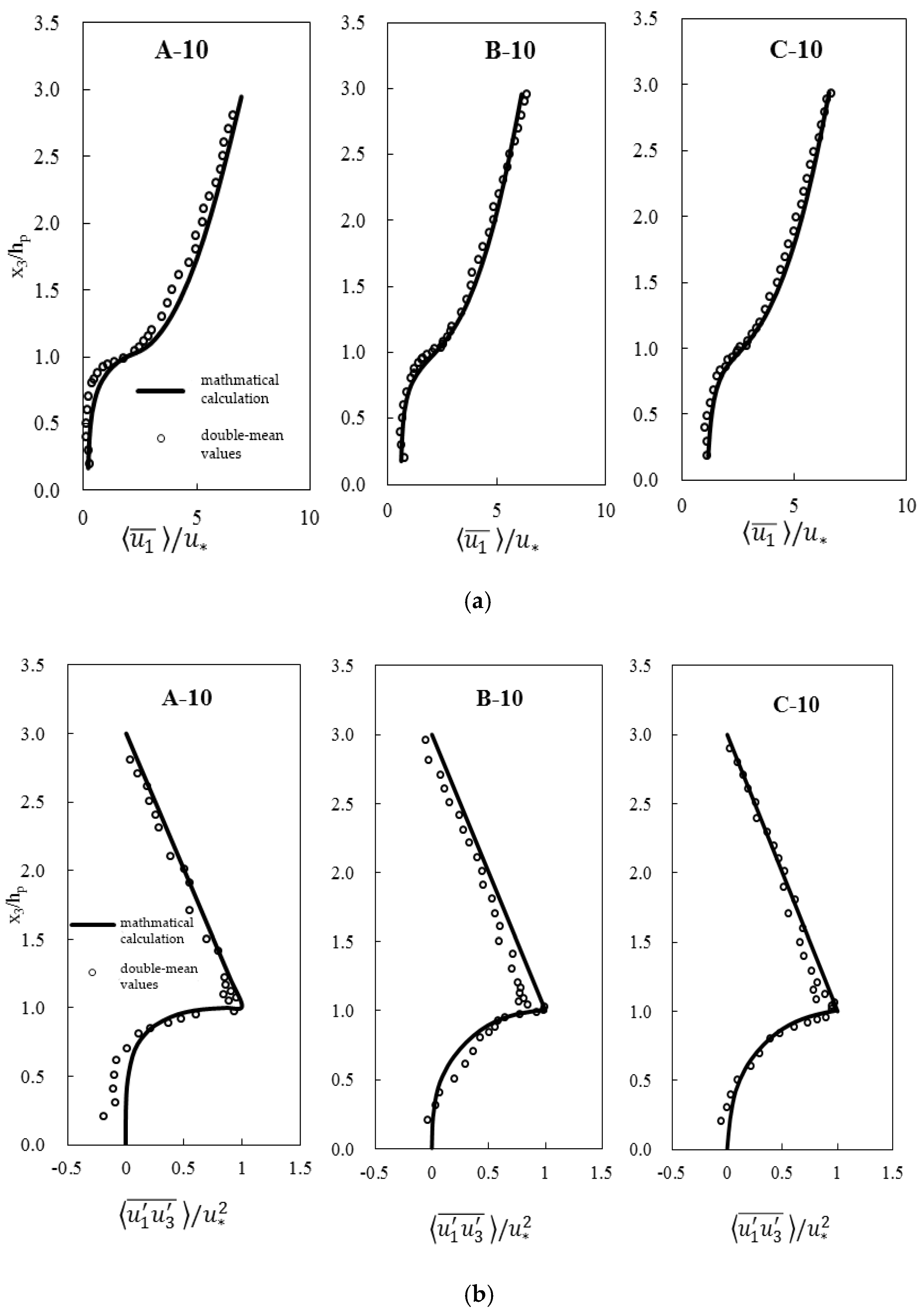
The flume in the experiment of Nezu et al. [4] was 10 m long and 0.4 m wide. Thin sheets of plastic (5 cm high, 0.8 cm wide and 0.1 cm thick) were used to simulate vegetation. Plastic sheets were arranged in rows in the 9 m long experimental section. An LDA and PIV were used to measure the flow velocity under different vegetation densities. The measurement vertical lines were arranged 7 m behind the entrance of the experimental area to ensure that the flow fully developed to be two-dimensional turbulence. Three data series were selected for verification calculation, which were measured in high Reynolds number conditions (A-10, B-10 and C-10) by the LDA. Vertical distribution of velocity and Reynolds stress data were used to verify. The main flow features of the experiments used to validate the mathematical model are shown in Table 1.
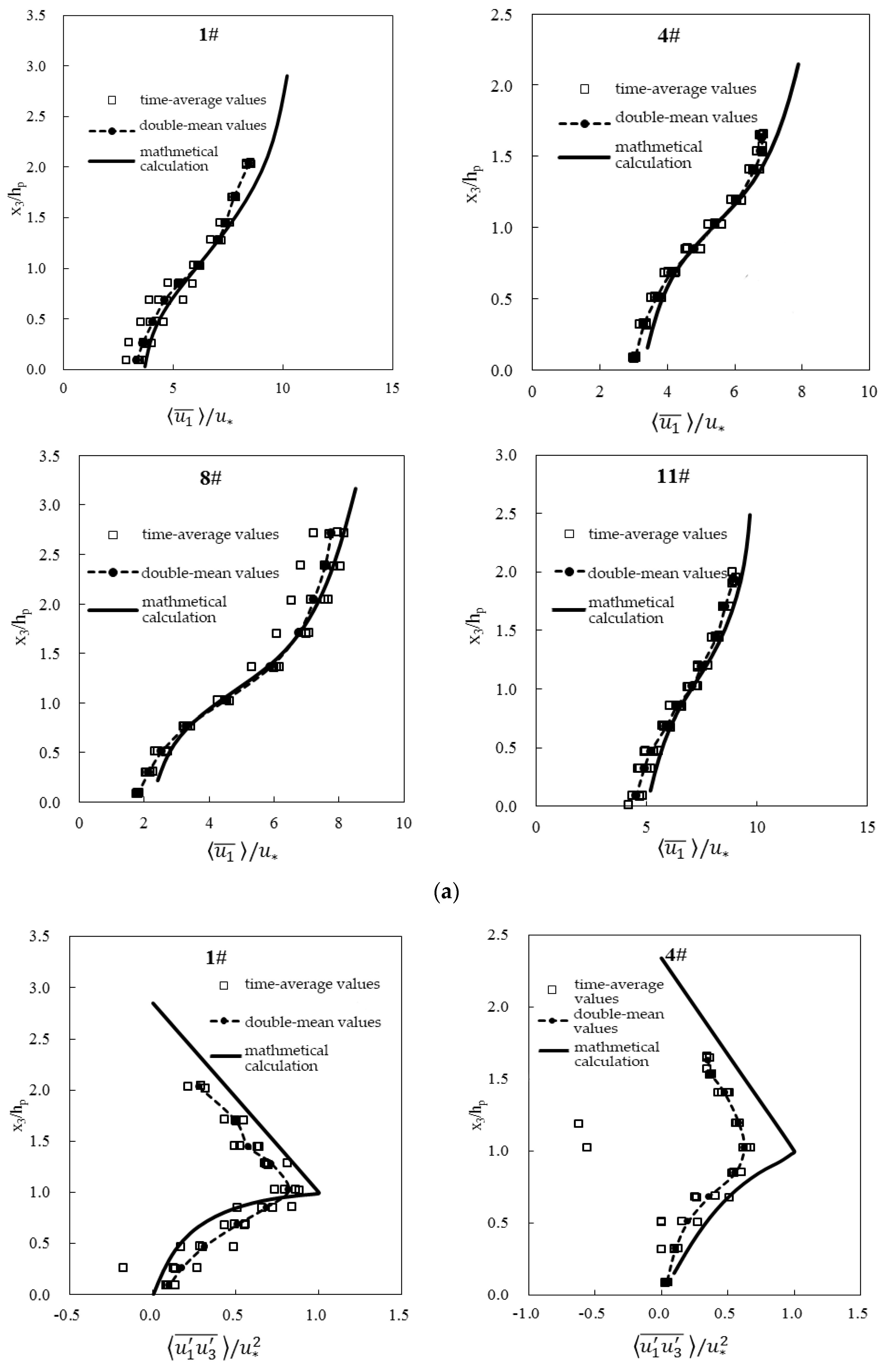
The experiments in Dunn et al. [1] were carried out in an experimental flume with a length of 19.50 m, a width of 0.91 m and a depth of 0.61 m. The flume was long enough to form uniform flow in the middle section. Wooden sticks with a diameter of 0.64 cm and a height of 12 cm were staggered in the water flume to simulate rigid vegetation. The flow velocity was measured by ADV. Ten groups of data under different experimental conditions were verified, including vertical distribution of velocity and Reynolds stress data. The main flow features of the experiments used to validate the mathematical model are shown in Table 2.
2.2. Study of the Water-Blocking Effect Generalization of Submerged Vegetation
For uniformly distributed submerged vegetation, the vegetation density, a, is an important parameter to generalize its influence (Dunn et al. [1]). The definition is formulated as follows:
where
: vegetation density (1/m);
: inflow area of a single cylinder (m2);
: volume affected by a single cylinder (m3);
: diameter of the cylinder (m);
: height of submerged vegetation (m);
: length of the volume in direction when averaged locally (m), and can be streamwise direction and spanwise direction, respectively;
: length of the volume in direction when averaged locally (m).
To describe the effect of submerged vegetation, we multiply vegetation density, a, by the height of submerged vegetation, h, and then divide it by water depth, H, creating a comprehensive parameter ah/H to describe the water-blocking effect of submerged vegetation on water. The larger ah/H is, the stronger resistance vegetation act on water, i.e., the denser the vegetation groups are. Otherwise, the sparser the vegetation groups are.
2.2.1. Generalization Model and Principle
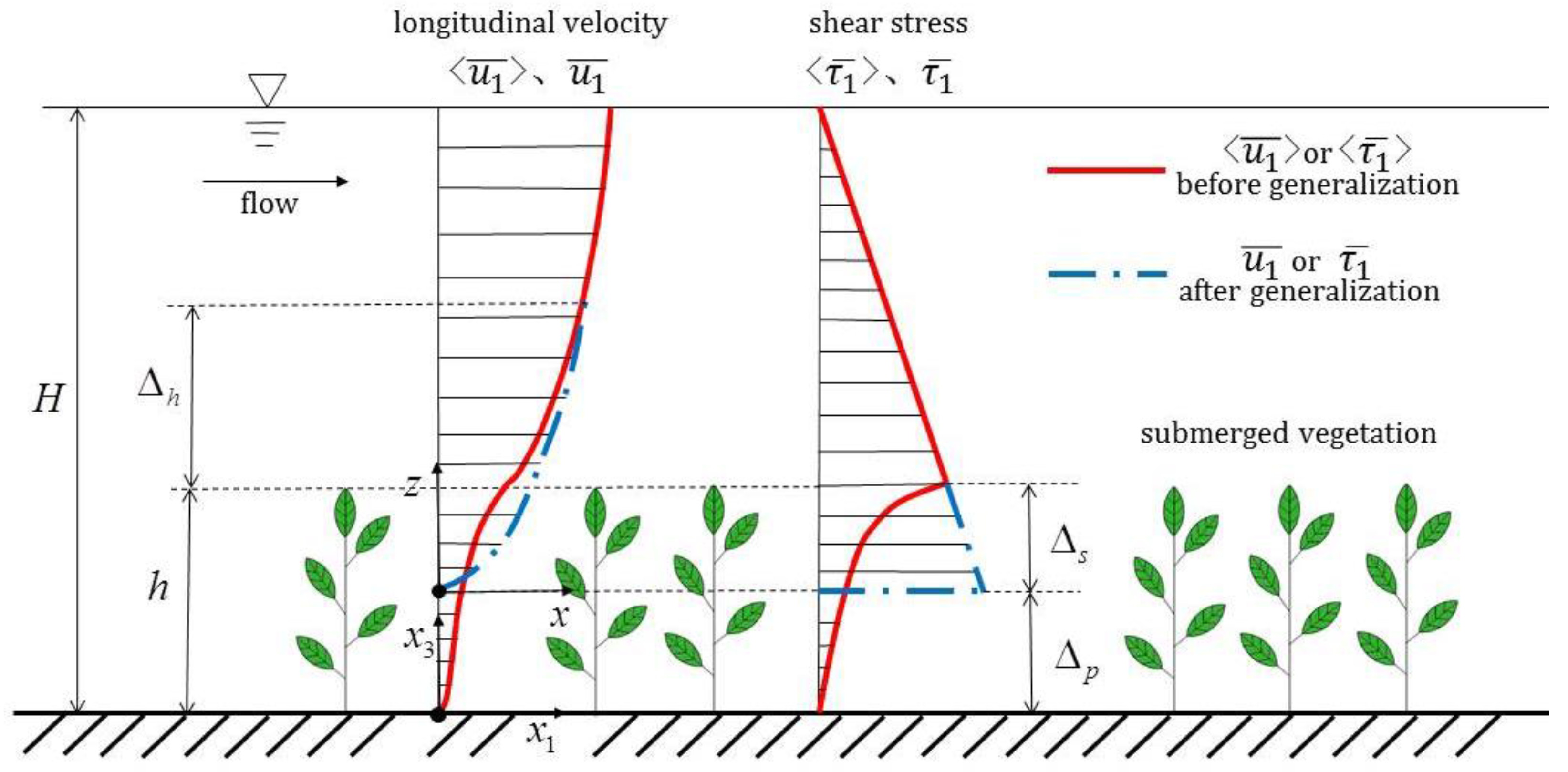
Based on the above numerical simulation results of the double-average velocity and Reynolds stress of open channel flow with submerged vegetation, the water-blocking effect of submerged vegetation is generalized by adjusting the position of the lower boundary and modifying the roughness coefficient, as shown in Figure 1. Here, the meaning of “generalization” can be explained as: the original complex flow field model of submerged vegetation open channel flow is simplified into a simple flow field model to ensure that before and after simplification, the water-blocking effect remains equivalent. In this way, it is convenient to use the generalized simple flow field model parameters to do engineering calculation. In Figure 1, Δs is the height of the theoretical zero point, and the flow velocity here is zero after generalization; Δp is the height of the equivalent virtual obstacle after generalization, and it’s called virtual channel height; Δh is the thickness of the affected region in which submerged vegetation changes the longitudinal velocity above the top of vegetation; and Δs + Δh is defined as the influence depth. Before generalization, the real flow is the pore flow in the vegetation layer and the free flow above the vegetation layer, both of which are described uniformly by means of double averaging. However, flow after generalization (called generalized flow) is constant uniform flow in the open channel described by the Reynolds average method. The latter’s effective water depth Hm can be defined as Hm = H − h + Δs.
The principles of generalizing the water-blocking effect of submerged vegetation are as follows:
(1) The quantity of flow before generalization equals that after generalization. This is required by the conservation of mass. As shown in Figure 1, the equation applies:
In Equation (11), Δs is the height discrepancy from the theoretical zero point of velocity (i.e., the top of virtual channel after generalization) to the top of the submerged vegetation layer.
(2) At the top of the influence depth (i.e., z = Δh + Δs), the double-average velocity before generalization equals the velocity after generalization.
2.2.2. Handling of Key Issues
In the process of solving Equations (11) and (12) to calculate Δs and Δh, the following problems need to be solved. One is the vertical distribution of the longitudinal velocity of the constant uniform flow, which is generated after generalization. In this paper, we choose the logarithmic velocity distribution formula (the constant shear stress hypothesis is also used, i.e., ). The other is that many flow characteristic variables after generalization are interrelated and need a coupling solution. This paper uses the following methods to obtain simultaneous equations.
(1) At x3 = Δp = h − Δs, , i.e., the theoretical zero point of velocity is at the place of x3 = Δp. Let z = x3 − Δp, and take the theoretical zero point as the origin to establish a new coordinate axis z. Then, the flow velocity distribution after generalization is:
Because at z = 0, , we further obtain
We substitute Equation (13) into Equation (11) to obtain
(2) Above the top of influence depth, i.e., z > Δh + Δs, the flow velocity after generalization equals that before generalization. In the calculation process, the absolute value of the difference between the two is set to be less than a minimal value εm. That is, 0
where i represents the velocity data i above the top of the influence depth. i = 1, 2, …, m. Here, is the absolute value of the difference between velocity data i before generalization and that after generalization. m is the total number of velocity data points above the top of the influence depth.
(3) According to the generalization of the shear stress distribution in Figure 1, we take
In Equation (17), τh and τb, respectively, represent the shear stress at the top of the vegetation layer before generalization and the shear stress at the top of the virtual channel after generalization. We take β = 0.75 (determined after trial). By combining Equations (15)–(17), Δs, Δh and u*b can be solved. The roughness coefficient np is determined by the Chezy formula:
Then,
In Equation (19), Hm is the effective water depth (the definition is in Section 2.2.1), , Q is the flow discharge quantity, B is the channel width, and g is the acceleration of gravity.
2.2.3. Data for Generalization
Among the published experimental data, Dunn et al. [1] is relatively systematic and complete. The 9 series of experimental velocity data from Dunn et al. [1] in different working conditions were selected for double-average treatment and numerical calculation, and then, the water-blocking generalization mentioned above was carried out using these data.
3. Results
3.1. Numerical Simulation of Open Channel Flow with Submerged Vegetation
3.1.1. Verification 1
As shown in Figure 2, the calculated results were in good agreement with the experimental results. Figure 2 presents the verification calculation results of the vertical distribution of velocity and Reynolds stress. The dimensionless results are obtained after original results being divided by the frictional velocity at the top of the vegetation layer, and are plotted in the figure. The frictional velocity is defined as .
3.1.2. Verification 2
3.2. Water-Blocking Effect Generalization of Submerged Vegetation
3.2.1. Preliminary Result
Figure 4 shows the comparison between the double-average velocity and generalized velocity in different working conditions. Figure 4 verifies the accuracy of the generalization mode shown in Figure 1. Illustrations in Figure 4: Δp is the height of the generalized obstacle—the virtual channel after generalization. At this height, the generalized flow velocity is zero. From here up, the generalized flow velocity increases from zero. When it rises to the height of vegetation, h, the generalized flow velocity still does not recover to the original flow velocity due to the effect of vegetation obstruction. The height difference in this section is the theoretical zero point’s height of the velocity, Δs. Then continue to rise to the highest dotted line, generalized flow velocity adjustment is completed, and it returns to the original flow velocity. That is, these two kinds of velocity overlap. The height difference of this section is the influence thickness, Δh. Then these two kinds of flow velocity remain consistently overlap, basically restore the original flow.
The results for the theoretical zero point’s position and roughness coefficient are introduced below.
3.2.2. Height of the Theoretical Zero Point Δs
The height of the theoretical zero point Δs is nondimensionalized by vegetation height h, and a dimensionless parameter Δs/h is obtained. Figure 5 shows the relationship between Δs/h and ah/H. The fitting formula is
Figure 5 and Equation (20) show a trend of gradually decreasing Δs/h with increasing ah/H. That is, when the water depth H and vegetation height h remain unchanged, the denser the vegetation arrangement is, the higher the theoretical zero point (in other words, the top of virtual channel rises higher). Analysis for the reason: increasing ah/H means a denser vegetation arrangement. Then, there is more resistance to the flow, and the water-blocking effect of vegetation is strengthened. After the generalization, the relative height of virtual channel (Δp/h) will increase. Accordingly, the relative height of the theoretical zero point (Δs/h) goes down. When ah/H is zero, there is no vegetation holding back water, so there is no virtual channel after generalization. That is, the virtual channel height Δp is zero. Then, the theoretical zero point’s height Δs is equal to the height of vegetation, h. Therefore, the y-coordinate value is zero. The extension prediction of fitting line accords with the actual law. The fitting line is suitable to express the relation between vegetation density and generalization results.
Figure 5 shows the variation trend of Δs. Here, Δp = h − Δs, so we can obtain the variation trend of Δp. Virtual channel elevation Δp is an important parameter obtained after generalization of water-blocking effect. Because it can be directly put into the plane two-dimensional model for engineering calculation.
3.2.3. Influence Depth Δs + Δh
The influence depth Δs + Δh is nondimensionalized by vegetation height h. Figure 6 shows the (Δs + Δh)/h~ah/H graph. The fitting formula is
As shown in Figure 6 and Equation (21), in the case of the same vegetation height h, the denser the vegetation arrangement is, the smaller the influence depth Δs + Δh is. Further analysis: similarly, the greater ah/H, the stronger the water-blocking effect of vegetation. Then, the water needs a higher depth in the vertical direction to restore its original flow. Therefore, the greater the range of influence thickness zone is, i.e., the greater Δh is. However, the actual increase amplitude of influence thickness, Δh, is small. This is related to the change in the influence depth, Δh + Δs, subsequently. According to Section 3.2.2, the smaller the theoretical zero point’s height Δs is, and the reduction is greater than the increase in Δh. Therefore, the influence depth Δs + Δh shows a decreasing trend as a whole. The height of vegetation h is fixed, so the ordinate value in Figure 6 shows a decreasing trend. When the abscissa value in the Figure 6 is −4, the extension value of the fitting line is exactly about 1. In addition, the relative value of the influence depth (Δs + Δh)/h is about e. In other words, in the condition of this vegetation arrangement, the influence depth Δs + Δh is about e times of the height of vegetation h (about 2.72 times).
3.2.4. Generalized Roughness Coefficient np
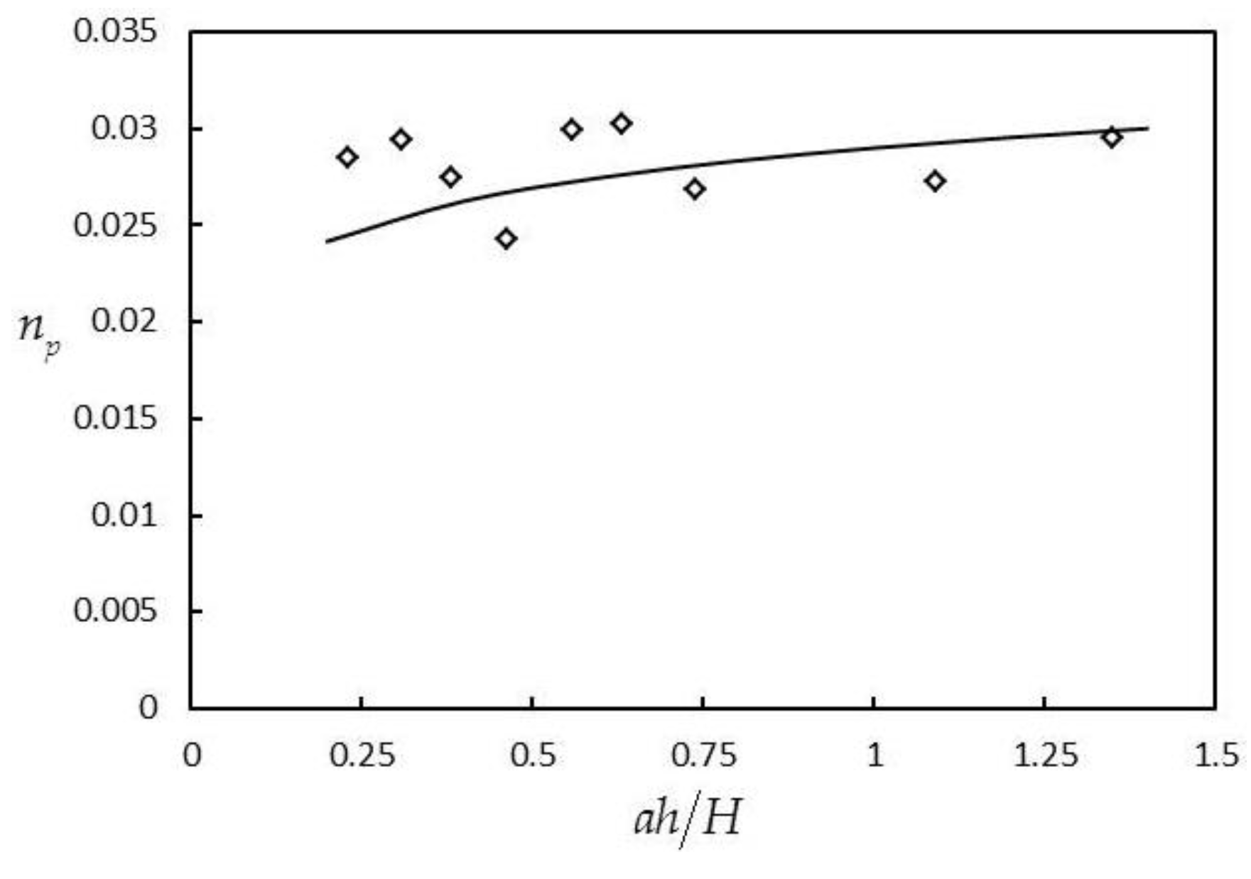
Figure 7 shows the calculation results of generalized roughness coefficient np. Here, np calculated from the experimental data in Dunn et al. [1] basically remains at approximately 0.029. However, there is also a trend of a slight increase in np with increasing ah/H. The denser the vegetation arrangement is, the higher generalized roughness coefficient np is. The fitting formula is
As shown in Figure 7 and Equation (22), the denser the vegetation arrangement is, the greater the generalized roughness coefficient np is. Because of the dense vegetation arrangement, the water-blocking effect of vegetation will be enhanced. Then the equivalent roughness coefficient after generalization, np, will increase.
The generalized roughness coefficient np is another important parameter obtained after generalization of water-blocking effect. Because it can also be directly put into plane two-dimensional model for engineering calculation.
3.2.5. Ratio of Single-Width-Discharges q/q0
The influence of submerged vegetation on discharge capacity is further analyzed by using the generalization results of the water-blocking effect mentioned above. Here, q and q0 represent the single-width discharge of open channel flow with or without submerged vegetation, respectively. The following formula can be obtained.
We further obtain:
We substitute np and Δs (from Figure 5 and Figure 7) into Equation (25) to obtain the calculated values of q/q0. Figure 8 shows the variation in q/q0 with the changes in ah/H. The corresponding experimental values of q/q0 (data from the experiment performed by Dunn et al. [1]) are also given in Figure 8. We also extend the calculated values of q/q0. Figure 8 shows the following: (1) The calculated values are basically consistent with the experimental values of Dunn et al. [1]. This shows that the calculation method of the water-blocking effect proposed in this paper has high precision; (2) q/q0 decreases monotonically with increasing ah/H. This result shows that the denser the submerged vegetation is or the higher the submerged vegetation is, the greater the discharge capacity decreases. This is in line with the objective law. Because of the dense vegetation arrangement, the water-blocking effect of vegetation will be enhanced. That is, the flow of water becomes more obstructed. With the decrease in flow velocity and flow space, the single-width-discharge, q, will become smaller. Then, divided by the single-width-discharge without vegetation obstruction, i.e., q0, the single-width-discharges ratio q/q0 will decrease. That is, the flow loss will increase, so Figure 8 shows a downward trend. It can be seen from Figure 8 that the cut-off point is the single-width-discharges ratio q/q0 equals to 0.4 (ah/H equals to about 0.75). Before and after this cut-off point, the single-width-discharges ratio q/q0 changes from fast to slow. When ah/H is zero, that is, there is no vegetation obstruction, the single-width-discharges ratio q/q0 is equal to 1. There is no flow loss, in line with the objective law. When ah/H is between 0 and 0.75, the single-width-discharge loss is rapid. (q/q0 rapidly decreases from 1 to 0.4. ah/H as short as 0.75 range, the single-width-discharge loses 60%.) It can be seen that in the early stage of vegetation density increase, a little change in vegetation density will cause a large loss of single-width-discharge. When ah/H is greater than 0.75, the single-width-discharge loss slows down. Over a long ah/H interval, the single-width-discharge ratio q/q0 only decreases from 0.4 to 0.2. That is, the single-width-discharge loss only increases by 20%. This is a stable interval of high loss rate of single-width-discharge. It can be seen that after the early stage of vegetation density increase, even if vegetation density increases again, it has little impact on the loss of single-width-discharge. Figure 8 can be used as a reference for estimating single-width-discharge variation and loss under the action of vegetation arrangement parameter, ah/H.
3.2.6. Comparison Results Related to Velocity Integration
The above is the water-blocking-effect generalization calculation for numerically simulated velocity. Then, the original velocity data were also generalized by the same way. Dunn et al. [1] conducted 18 groups of experiments, each of which measured data in four random cross sections. The original velocity data of these random sections were generalized with the same method mentioned above. Then we calculated four parameters: Δs, Δs + Δh, np, q/q0. The velocity of four sections is different, so the single-width discharge of each section is calculated (i.e., the integral area of the velocity distribution diagram). These four sections are then sorted by the size of the single-width discharge in every group, labeled in descending order as Max1, Max2, Max3, and Max4. Then the influence of velocity integral areas in four sections on the four parameters is explored.
(1) Height of the Theoretical Zero Point Δs
Figure 9 shows the result of theoretical zero point height ∆s, which is calculated after generalization using original flow velocity data. Then, ∆s is also nondimensionalized in the same way. Figure 9 shows that: (1) When using original velocity to be generalized, the overall trend of the parameter ∆s is consistent with that of the numerical calculation velocity in Section 3.2.2, i.e., both show a decreasing trend of ∆s/h with the increase in ah/H. That is, when water depth H and vegetation height h remain unchanged, the denser vegetation layout is, the higher the theoretical zero point is (the higher virtual channel upper boundary is lifted). (2) For the same ah/H, the larger the integrated area of the flow velocity is, or say the single width flow discharge increases, (Max1 blue line is the largest, Max4 purple line is the smallest), the larger parameter Δs is, and the smaller it is otherwise. Further analysis for (2): for the same ah/H (i.e., the same group), although water depth H is equal, the greater integrated area of flow velocity in four cross sections is, the larger velocity value is, meaning flow moves faster. Therefore, the generalized virtual channel will be lower, i.e., Δp will be smaller, and the corresponding proportion Δp/h will be smaller too. Thus, faster flow can be allowed. Accordingly, the proportion of theoretical zero point height, Δs/h, is larger.
As seen in Figure 9, the relationship between velocity integration and theoretical zero point height is positive. Because Δp = h − Δs, the relationship between velocity integration and virtual channel elevation is negative.
(2) Influence Depth Δs + Δh
Figure 10 shows the result of influence depth Δs + Δh, which is calculated after generalization using original flow velocity data. Then, Δs + Δh is also nondimensionalized by the same way. Figure 10 shows that: (1) when using original velocity to be generalized, the overall trend of the parameter Δs + Δh is consistent with that of the numerical calculation velocity in Section 3.2.3, i.e., both show a decreasing trend of (Δs + Δh)/h with the increase in ah/H. That is, when vegetation height h remains unchanged, the denser the vegetation layout is, the smaller the influence depth Δs + Δh is. (2) The greater the integrated area of flow velocity is, the larger the influence depth Δs + Δh is. Further analysis for (2): for the same ah/H (i.e., the same group), although the water depth H is equal, the greater the integrated area of flow velocity in four cross sections is, the larger the velocity value is, meaning the flow moves faster. Therefore, at the same h (i.e., at the same water-blocking height), the larger the generalized influence depth Δs + Δh will be, meaning that the water needs a higher depth in the vertical direction to restore its original flow. In other words, the water-blocking-effect is stronger. A stronger water-blocking-effect reflects a stronger force between the faster flow and the obstruction.
(3) Generalized Roughness Coefficient np
Figure 11 shows the result of generalized roughness coefficient np, which is calculated after generalization using original flow velocity data. Figure 11 shows that: (1) The magnitude of the parameter np in this section is basically the same as that of the numerical flow velocity in Section 3.2.4, but the variation with ah/H is smaller than that in Section 3.2.4, i.e., when ah/H increases, np increases weakly. (2) The greater integrated area of flow velocity is, the larger generalized roughness coefficient np is. Further analysis for (2): for the same ah/H (i.e., the same group), although the water depth H is equal, the greater the integrated area of flow velocity in four cross sections is, the larger the velocity value is, meaning the flow moves faster. Therefore, at the same h (i.e., at the same water-blocking height), the larger the generalized roughness coefficient np will be, meaning the water-blocking-effect will be stronger. As mentioned above, a stronger water-blocking-effect reflects a stronger force between the faster flow and the obstruction.
As seen in Figure 11, the relationship between velocity integration and generalized roughness coefficient np is positive.
(4) Ratio of Single-Width-Discharges q/q0
Figure 12 shows the result of ratio of single-width-discharges q/q0, which is calculated after generalization using original flow velocity data. Figure 12 shows that: (1) when using original velocity to be generalized, the overall trend of q/q0 is consistent with that of the numerical calculation velocity in Section 3.2.5, i.e., both show a decreasing trend of q/q0 with the increase in ah/H. That is, the denser the vegetation layout is, or the higher the vegetation is, the loss of discharge capacity is more significant. (2) The larger integrated area of the flow velocity is, the smaller generalized q/q0 is. Further analysis for (2): for the same ah/H (i.e., the same group), although the water depth H is equal, the greater the integrated area of flow velocity in four cross sections is, the larger the velocity value is, meaning the flow moves faster. Therefore, the force between faster flow and obstruction will be stronger. Then, energy loss will be greater as well. This is the reason why generalized q/q0 is smaller with the increase in the integrated area of the flow velocity.
It can be seen that even with the same ah/H, the difference in the integrated area of flow velocity (i.e., single-width discharge) can also affect the water-blocking-effect generalization results.
4. Discussion
The influence of numerical calculation and average treatment on the water-blocking-effect generalization is discussed below. Three cases are discussed, which are: original velocity is numerically calculated firstly, and then water-blocking-effect generalization is performed to obtain parameters (i.e., Section 3.2.2, Section 3.2.3, Section 3.2.4 and Section 3.2.5); original velocity is generalized firstly to obtain original parameters, and then these original parameters are averaged (i.e., Section 3.2.6); original velocity is firstly treated by double-average method and then water-blocking-effect generalized to obtain parameters. Finally, we discuss four parameters (i.e., Δs, Δs + Δh, np and q/q0) from three cases mentioned above.
4.1. Height of the Theoretical Zero Point Δs in Three Cases
The theoretical zero height Δs processed in three cases, and the fitting line obtained in Section 3.2.2 (here called the central line) are drawn into the coordinates together, as shown in Figure 13 below.
It can be seen from Figure 13 that: (1) The results of three cases have the same overall trend. The larger the ah/H is, the smaller the Δs/h is. That is, with the dense vegetation layout, the theoretical zero height Δs is smaller, and the virtual channel after generalization is elevated (i.e., Δp is larger). (2) Comparing three cases’ data, those of numerical calculation (case 1) are scattered and deviate most from the central line. Data of other two cases (case 2 and case 3) are concentrated relatively. It shows that the two mean-methods can better reflect the central trend. (3) There is little difference between data of case 2 and case 3, indicating that there is little difference between cases of first-generalization and first-averaging for this parameter Δs/h.
4.2. Influence Depth Δs + Δh in Three Cases
The influence depth Δs + Δh processed in three cases, and the fitting line obtained in Section 3.2.3 (here called the central line) are drawn into the coordinates together, as shown in Figure 14 below.
It can be seen from Figure 14 that: (1) the results of the three cases have the same general trend, the larger the ah/H is, the smaller the (Δs + Δh)/h is. The h in the figure is 0.1175 m, so (Δs + Δh) decreases with the increase in ah/H. (2) Comparing data in three cases, the difference is small, and they all concentrate around the central line. It shows that there is little difference among the three cases for reflecting the central trend.
4.3. Generalized Roughness Coefficient np in Three Cases
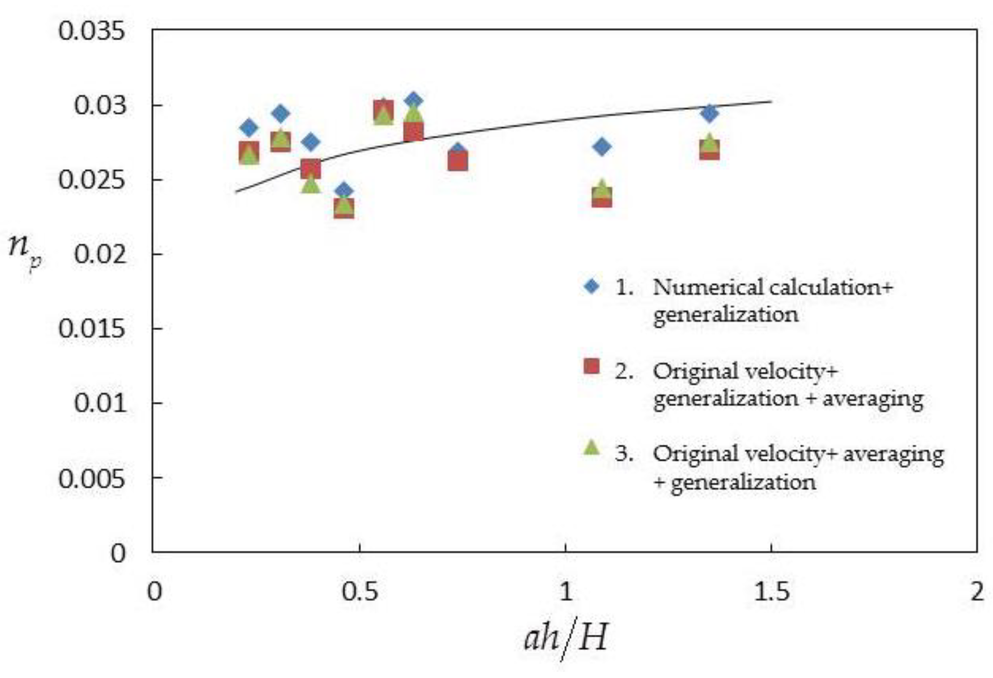
The generalized roughness coefficient np processed in three cases, and the fitting lines obtained in Section 3.2.4 (here called the central line) are drawn into the coordinates together, as shown in Figure 15 below.
It can be seen from Figure 15 that: (1) The results of the three cases have the same general trend, the larger ah/H is, the larger np is. That is, with the dense vegetation layout, the generalized roughness coefficient np is larger, and all data generally distribute around the center line. (2) Comparing data in three cases, data in case 1 (i.e., numerical calculation data) are relatively larger. Data in case 2 and case 3 are relatively smaller and there is little difference between them. It shows that data processed by numerical calculation are larger than those processed by mean calculation, and there is little difference between the two latter cases.
4.4. Ratio of Single-Width-Discharges q/q0 in Three Cases
The ratio of single-width-discharges q/q0 processed in three cases, and the calculated line obtained in Section 3.2.5 (here called the central line) are drawn into the coordinates together, as shown in Figure 16 below.
It can be seen from Figure 16 that: (1) the results of the three cases have the same general trend, the smaller ah/H is, the larger q/q0 is. That is, with the sparse vegetation layout, smaller flow discharge loss is, and all data generally distribute around the center line. (2) Comparing data in three cases, data in case 2 and case 3 (i.e., mean calculation cases) are generally equal. Data in case 1 are also generally equal to that of case 2 and case 3, except two are relatively smaller. Therefore, we can basically say that there is little difference in q/q0 of three cases, and they can all reflect the same center trend.
Brief summary of Section 4.1 to Section 4.4: average-treatment and numerical simulation treatment have effects on the comprehensive roughness coefficient and virtual channel elevation value, that is, they are different. In addition, average-treatment before or after water-blocking effect generalization makes little difference in the comprehensive roughness coefficient and virtual channel elevation.
4.5. Influences of Arrangement of Vegetation
A new mode for the description of field characteristics and general characteristics of submerged vegetation open channel flow is proposed in this article. In this work, space average method is used. This method can eliminate the effect of the arrangement of vegetation, whether it is regular or random. After space average method, specific arrangement forms can be further researched. That is, fine models of regular or random arrangements can be studied later. Therefore, a special research for this topic can be carried out. Moreover, submerged vegetation is complex in nature. To describe this complex morphology, porosity and water-blocking elevation are also considered in this article. In addition, flow with simple boundary conditions is studied. Then, other arrangement patterns will be studied in the next step. However, the generalized model is not affected by the arrangement mode, whether it is a regular or random arrangement. Therefore, in this work, regular arrangement is used to represent a common type of arrangement. Arrangement mode can be changed in the next step of more detailed research for fine models.
4.6. Discussion of Implications for Environmental Flows and Hydraulic Engineering Problems
The model in this manuscript can be used to calculate some environmental flows with submerged vegetation. For example, the numerical model can be used to determine sediment transport rates. The steps are as follows: Equations (1) and (4)–(6) are a set of equations. Four unknowns (ks, kw, εs, u1) are solved together. The numerical method is to discretize the equations using an unsteady finite volume method. Each equation is discretized as the governing equation of unsteady flow. Add the time partial derivative of the variable to the left-hand side of each governing equation. The central difference scheme is used to differentiate the time term. The flow is iteratively calculated with the number of steps in a certain time. In addition, then we put in the boundary conditions. In the boundary conditions, ks and εs are the same as the standard k-ε equation, and the gradient of the newly introduced kw is zero at the bottom of the open channel and on the free surface. Finally, Gauss–Seidel iterative method is used to solve discrete algebraic equations. After that, the longitudinal velocity profile of open channel flow with submerged vegetation is obtained. These velocity values can then be used to calculate shear stress and determine the sediment transport rates. There are other implications as well, for example, a lot of aquatic vegetation is morphologically distinct from rigid cylinders (they have leaves, branches, etc.), so this would probably modify the velocity and shear stress profiles from the examples provided in this manuscript. The distribution pattern of velocity and shear stress is greatly affected by vegetation form and water flow condition. It is suggested that readers should first find experiments of submerged vegetation with leaves and branches for flow velocity distribution if they are interested. In addition, then you can think about whether to decompose k and ε into two or more parts. Accordingly, the governing Equations (4)–(6) may introduce new parts of k and ε. The variable expression in the equation may need to change some coefficients’ values. Vegetation porosity is the main parameter.
This work has practical implications in real hydraulic engineering problems. The numerical simulation method proposed in this manuscript can be used to establish the corresponding model for the open channel flows with submerged vegetation, such as rivers, channels, and canals. Then the flow field can be predicted. The velocity and Reynolds stress distribution and sediment transport rates can be obtained. The generalization of the water-blocking effect can be used on basis of the numerical simulation to obtain generalized quantities. We can also consult the values of generalized quantities directly on the result charts with the specific value of comprehensive parameter ah/H, to obtain generalized quantities. These quantities can be calculated in the planar two-dimensional model or in the existing theory and general formulas of open channel flow. After these treatments, the overflow capacity and flood discharge capacity of vegetated open channels can be assessed and predicted, as well as the stabilization of sediment deposits inside riverbanks or in lateral embayments, and the shipping conditions of vegetated open channels. Submerged vegetation also has certain influences on channel morphology and stabilization of sediment deposits. The abundant vegetation in the riverbed can change the channel morphology into a wide and shallow form. For example, Southard et al. [28] have found that reaches with abundant bed vegetation are significantly wider (by an average of approximate to 50%), with shallower flows and lower velocities, than reaches with little bed vegetation. Dense submerged vegetation has the function of concentrating sediments, as found by Li et al. [29]: dense vegetation renders the vertical distribution profile uneven and captures sediment particles into the vegetation layer. Hyung et al. [30] also found that for certain flows, i.e., flows above the sediment motion threshold, sediment accumulated within and around the vegetation patch due to a reduction in bed shear stress. Vegetation-generated turbulence can cause an enhanced sediment transport, as pointed by Yang et al. [31]. In addition, sediment retention areas are formed by vegetation through baffling the flow and reducing the bed stress [32]. The generalization method proposed in this article can simplify original model and be applied to the calculation of channel morphology and sediments stability more conveniently.
5. Conclusions
Through theoretical analysis and numerical simulation, we discuss the flow field characteristics and generalization of the water-blocking effect of open channel flow with submerged vegetation, and draw the following conclusions:
(1) As the basis of generalization, in order to make up for the deficiency of experimental results, a new numerical simulation model for the flow field of submerged vegetation open channel flow was proposed before the main work. This is a simple model. The innovation is that the turbulence kinetic energy and the dissipation rate of turbulence kinetic energy in the model are decomposed into two parts, large-scale shear turbulence part and stem-scale turbulence part, respectively. The interaction between the two is considered through a transformation term. The verification results show that the model has high simulation accuracy.
(2) For the purpose of the study, a simple generalization model of the water-blocking effect of submerged vegetation was proposed. Finally, two parameters of generalized roughness coefficient and virtual channel elevation were obtained to reflect the water-blocking effect. They can be put directly into a planar two-dimensional model in engineering. It achieves the ultimate goal of convenient engineering calculation.
(3) The influence of velocity integration and average-treatment on the water-blocking effect generalization model of submerged vegetation is further studied. The relationship between velocity integration and generalized roughness coefficient is positive, and the relationship between velocity integration and virtual channel elevation is negative. Average-treatment and numerical simulation treatment have effects on the generalized roughness coefficient and virtual channel elevation value, that is, they are different. In addition, average-treatment before or after water-blocking effect generalization makes little difference in generalized roughness coefficient and virtual channel elevation.
Author Contributions
Conceptualization, C.Q., S.L. and W.P.; methodology, C.Q., S.L. and W.P.; formal analysis, C.Q., S.L. and W.P.; investigation, C.Q. and W.P.; resources, C.Q. and W.P.; data curation, C.Q. and W.P.; writing—original draft preparation, C.Q., S.L. and W.P.; writing—review and editing, C.Q., S.L. and W.P.; visualization, C.Q. and W.P.; supervision, S.L. and J.H.; project administration, S.L.; funding acquisition, S.L. All authors have read and agreed to the published version of the manuscript.
Funding
This research was funded by Ministry of Science and Technology of the People’s Republic of China, the National Key R&D Program of China, grant number 2018YFC0407600.
Institutional Review Board Statement
Not applicable.
Informed Consent Statement
Not applicable.
Data Availability Statement
The data presented in this study are available on request from authors.
Acknowledgments
The authors would like to express their gratitude to Changjiang River Scientific Research Institute.
Conflicts of Interest
The authors declare no conflict of interest. The funders had no role in the design of the study; in the collection, analyses, or interpretation of data; in the writing of the manuscript; or in the decision to publish the results.
Abbreviations
| Symbol Key | |
| instantaneous variable | |
| time mean variable | |
| fluctuation variable | |
| local spatial mean | |
| local spatial pulsation | |
| longitudinal flow velocity after double averaging (m/s) | |
| longitudinal flow velocity after generalization (m/s) | |
| shear stress after double averaging (Pa) | |
| shear stress after generalization (Pa) | |
| bottom slope of the open channel | |
| diameter of submerged vegetation (m) | |
| porosity of the flora | |
| drag coefficient | |
| molecular viscosity coefficient (m2/s) | |
| turbulence viscosity coefficient (m2/s) | |
| k | turbulent kinetic energy |
| ks | turbulent kinetic energy of the large-scale shear turbulence |
| kw | turbulent kinetic energy of the small-scale stem turbulence |
| ε | turbulent kinetic energy dissipation rate |
| εs | turbulent kinetic energy dissipation rate of the large-scale shear turbulence |
| εw | turbulent kinetic energy dissipation rate of the small-scale stem turbulence |
| WD | a term reflecting the transformation of shear turbulent kinetic energy to stem-scale wake kinetic energy |
| νt | turbulent viscosity coefficient |
| vegetation density (1/m) | |
| inflow area of a single cylinder (m2) | |
| volume affected by a single cylinder (m3) | |
| diameter of the cylinder (m) | |
| height of submerged vegetation (m) | |
| length of the volume in direction when averaged locally (m), and can be streamwise direction and spanwise direction, respectively. | |
| length of the volume in direction when averaged locally (m). | |
| ah/H | a comprehensive parameter to describe the water-blocking effect of submerged vegetation on water (1/m) |
| Δs | the height of the theoretical zero point, and the flow velocity here is zero after generalization (m) |
| Δp | the height of the equivalent virtual obstacle after generalization, and it’s called virtual channel height (m) |
| Δh | the thickness of the affected region in which submerged vegetation changes the longitudinal velocity above the top of vegetation (m) |
| Δs + Δh | the influence depth (m) |
| Hm | effective water depth (m), defined as Hm = H − h + Δs |
| τh | shear stress at the top of the vegetation layer before generalization (Pa) |
| τb | shear stress at the top of the virtual channel after generalization (Pa) |
| np | roughness coefficient |
| Q | flow discharge quantity (m3/s) |
| B | channel width (m) |
| g | the acceleration of gravity (m2/s) |
| frictional velocity (m/s), defined as | |
| q | single-width discharge of open channel flow with submerged vegetation (m3/s) |
| q0 | single-width discharge of open channel flow without submerged vegetation (m3/s) |
References
- Chad, D.; Fabian, L.; Marcelo, G. Mean flow and turbulence in a laboratory channel with simulated vegetation. In Civil Engineering Studies; Hydrosystems Laboratory, Department of Civil Engineering, University of Illinois at Urbana–Champaign: Urbana, IL, USA, 1996; Hydraulic Engineering Series No. 51. [Google Scholar]
- Raupach, M.R.; Finnigan, J.J.; Brunei, Y. Coherent eddies and turbulence in vegetation canopies: The mixing-layer analogy. Bound-Layer Meteorol. 1996, 78, 351–382. [Google Scholar] [CrossRef]
- Nepf, H.; Ghisalberti, M.; White, B.; Murphy, E. Retention time and dispersion associated with submerged aquatic canopies. Water Resour. Res. 2007, 43, 436–451. [Google Scholar] [CrossRef]
- Iehisa, N.; Michio, S. Turburence structure and coherent motion in vegetated canopy open-channel flows. J. Hydro-Environ. Res. 2008, 2, 62–90. [Google Scholar]
- Carmelo, J.; Schärer, C.; Jenny, H.; Schleiss, A.J.; Franca, M.J. Floodplain land cover and flow hydrodynamic control of overbank sedimentation in compound channel flows. Water Resour. Res. 2019, 55, 9072–9091. [Google Scholar]
- Vargas-Luna, A.; Duró, G.; Crosato, A.; Uijttewaal, W. Morphological adaptation of river channels to vegetation establishment: A laboratory study. J. Geophys. Res.-Earth 2019, 124, 1981–1995. [Google Scholar] [CrossRef] [Green Version]
- Nepf, H.M.; Vivoni, E.R. Flow structure in depth-limited, vegetated flow. J. Geophys. Res.-Oceans 2000, 105, 28547–28557. [Google Scholar] [CrossRef]
- Ghisalberti, M.; Nepf, H. Shallow flows over a permeable medium: The hydrodynamics of submerged aquatic canopies. Transp. Porous Med. 2009, 78, 309–326. [Google Scholar] [CrossRef]
- Ortiz, A.C.; Ashton, A.; Nepf, H. Mean and turbulent velocity fields near rigid and flexible plants and the implications for deposition. J. Geophys. Res.-Earth 2013, 118, 2585–2599. [Google Scholar] [CrossRef]
- Ghisalberti, M. Mixing layers and coherent structures in vegetated aquatic flows. J. Geophys. Res. 2002, 107, 3011. [Google Scholar] [CrossRef]
- Ghisalberti, M.; Nepf, H.M. The limited growth of vegetated shear layers. Water Resour. Res. 2004, 40, 196–212. [Google Scholar] [CrossRef]
- Ghisalberti, M.; Schlosser, T. Vortex generation in oscillatory canopy flow. J. Geophys. Res.-Oceans 2013, 118, 1534–1542. [Google Scholar] [CrossRef]
- Takaaki, O.; Iehisa, N.; Michio, S. Flow-vegetation interactions: Length-scale of the “monami” phenomenon. J. Hydraul. Res. 2016, 54, 251–262. [Google Scholar]
- Takaaki, O.; Iehisa, N. Spatial evolution of coherent motions in finite-length vegetation patch flow. Environ. Fluid Mech. 2013, 13, 417–434. [Google Scholar]
- Zeng, Y.; Huai, W.; Zhao, M. Flow characteristics of rectangular open channels with compound vegetation roughness. Appl. Math. Mech. 2016, 37, 341–348. [Google Scholar] [CrossRef]
- Coceal, O.; Dobre, A.; Thomas, T.G. Unsteady dynamics and organized structures from dns over an idealized building canopy. Int. J. Climatol. 2007, 27, 1943–1953. [Google Scholar] [CrossRef] [Green Version]
- Ji, C.; Munjiza, A.; Williams, J.J.R. A novel iterative direct-forcing immersed boundary method and its finite volume applications. J. Comput. Phys. 2012, 231, 1797–1821. [Google Scholar] [CrossRef]
- Choi, S.U.; Kang, H. Numerical investigations of mean flow and turbulence structures of partly-vegetated open-channel flows using the Reynolds stress model. J. Hydraul. Res. 2006, 44, 203–217. [Google Scholar] [CrossRef]
- Kang, H.; Choi, S.U. Turbulence modeling of compound open-channel flows with and without vegetation on the floodplain using the Reynolds stress model. Adv. Water Resour. 2006, 29, 1650–1664. [Google Scholar] [CrossRef]
- Coceal, O.; Thomas, T.G.; Castro, I.P.; Belcher, S.E. Mean Flow and Turbulence Statistics over Groups of Urban-like Cubical Obstacles. Bound-Layer Meteorol. 2006, 121, 491–519. [Google Scholar] [CrossRef]
- Defina, A.; Bixio, A.C. Mean flow and turbulence in vegetated open channel flow. Water Resour. Res. 2005, 41, 372–380. [Google Scholar] [CrossRef] [Green Version]
- Huai, W.; Song, S.; Han, J.; Zeng, Y. Prediction of velocity distribution in straight open-channel flow with partial vegetation by singular perturbation method. Appl. Math. Mech. 2016, 37, 1315–1324. [Google Scholar] [CrossRef]
- Bai, F.; Yang, Z.; Huai, W.; Zheng, C. A depth-averaged two dimensional shallow water model to simulate flow-rigid vegetation interactions. In Proceedings of the 12th International Conference on Hydroinformatics (HIC)—Smart Water for the Future, Incheon, Republic of Korea, 21–26 August 2016. [Google Scholar]
- Luhar, M.; Nepf, H.M. From the blade scale to the reach scale: A characterization of aquatic vegetative drag. Adv. Water Resour. 2013, 51, 305–316. [Google Scholar] [CrossRef]
- Murphy, E.; Ghisalberti, M.; Nepf, H. Model and laboratory study of dispersion in flows with submerged vegetation. Water Resour. Res. 2007, 43, 1315–1324. [Google Scholar] [CrossRef]
- Hu, Y.; Huai, W.; Han, J. Analytical solution for vertical profile of streamwise velocity in open-channel flow with submerged vegetation. Environ. Fluid Mech. 2013, 13, 389–402. [Google Scholar] [CrossRef]
- Shi, H.; Liang, X.; Huai, W.; Wang, Y. Predicting the bulk average velocity of open-channel flow with submerged rigid vegetation. J. Hydrol. 2019, 572, 213–225. [Google Scholar] [CrossRef]
- Southard, P.; Johnson, J.; Rempe, D.; Matheny, A. Impacts of Vegetation on Dryland River Morphology: Insights from Spring-Fed Channel Reaches, Henry Mountains, Utah. Water Resour. Res. 2022, 58, e2021WR031701. [Google Scholar] [CrossRef]
- Li, D.; Yang, Z.; Sun, Z.; Huai, W.; Liu, J. Theoretical Model of Suspended Sediment Concentration in a Flow with Submerged Vegetation. Water 2018, 10, 1656. [Google Scholar] [CrossRef] [Green Version]
- Kim, H.; Kimura, I.; Shimizu, Y. Bed morphological changes around a finite patch of vegetation. Earth Surf. Process. Landf. 2015, 40, 375–388. [Google Scholar] [CrossRef]
- Yang, J.; Nepf, H. A Turbulence-Based Bed-Load Transport Model for Bare and Vegetated Channels. Geophys. Res. Lett. 2018, 45, 10428–10436. [Google Scholar] [CrossRef]
- Cotton, J.; Wharton, G.; Bass, J.; Heppell, C.; Wotton, R. The effects of seasonal changes to in-stream vegetation cover on patterns of flow and accumulation of sediment. Geomorphology 2006, 77, 320–334. [Google Scholar] [CrossRef]
Figure 1.
Generalization of flow longitudinal velocity and shear stress.

Figure 2.
Verification calculation results of the double-mean longitudinal velocity and Reynolds stress (experimental data source: Nezu et al. [4]): (a) verification calculation results of the double mean longitudinal velocity; (b) verification calculation results of the double-mean Reynolds stress.

Figure 3.
Verification calculation results of the double-mean longitudinal velocity and Reynolds stress (experimental data source: Dunn et al. [1]): (a) verification calculation results of the double mean longitudinal velocity; (b) verification calculation results of the double-mean Reynolds stress.


Figure 4.
Comparison of the double-mean velocity and generalized velocity . (The upper dotted line is the depth of influence, the middle dotted line is the height of vegetation and the lower dotted line is the top of the virtual canal).
Figure 4.
Comparison of the double-mean velocity and generalized velocity . (The upper dotted line is the depth of influence, the middle dotted line is the height of vegetation and the lower dotted line is the top of the virtual canal).

Figure 5.
Height of the theoretical zero point Δs varies with the comprehensive parameter ah/H.

Figure 6.
Influence depth Δs + Δh varies with the comprehensive parameter ah/H.

Figure 7.
Generalized roughness coefficient np varies with the comprehensive parameter ah/H.

Figure 8.
Ratio of single-width-discharges q/q0 varies with the comprehensive parameter ah/H.

Figure 9.
Height of the theoretical zero point Δs varies with the comprehensive parameter ah/H. (calculated from original velocity data with different velocity integration in experiments of Dunn et al. [1]).
Figure 9.
Height of the theoretical zero point Δs varies with the comprehensive parameter ah/H. (calculated from original velocity data with different velocity integration in experiments of Dunn et al. [1]).

Figure 10.
Influence depth Δs + Δh varies with the comprehensive parameter ah/H. (calculated from original velocity data with different velocity integration in experiments of Dunn et al. [1]).
Figure 10.
Influence depth Δs + Δh varies with the comprehensive parameter ah/H. (calculated from original velocity data with different velocity integration in experiments of Dunn et al. [1]).

Figure 11.
Generalized roughness coefficient np varies with the comprehensive parameter ah/H. (calculated from original velocity data with different velocity integration in experiments of Dunn et al. [1]).
Figure 11.
Generalized roughness coefficient np varies with the comprehensive parameter ah/H. (calculated from original velocity data with different velocity integration in experiments of Dunn et al. [1]).

Figure 12.
Ratio of single-width-discharges q/q0 varies with the comprehensive parameter ah/H. (calculated from original velocity data with different velocity integration in experiments of Dunn et al. [1]).
Figure 12.
Ratio of single-width-discharges q/q0 varies with the comprehensive parameter ah/H. (calculated from original velocity data with different velocity integration in experiments of Dunn et al. [1]).

Figure 13.
Height of the theoretical zero point Δs varies with the comprehensive parameter ah/H (3 cases).
Figure 13.
Height of the theoretical zero point Δs varies with the comprehensive parameter ah/H (3 cases).

Figure 14.
Influence depth Δs + Δh varies with the comprehensive parameter ah/H. (3 cases).

Figure 15.
Generalized roughness coefficient np varies with the comprehensive parameter ah/H. (3 cases).
Figure 15.
Generalized roughness coefficient np varies with the comprehensive parameter ah/H. (3 cases).

Figure 16.
Ratio of single-width-discharges q/q0 varies with the comprehensive parameter ah/H. (3 cases).
Figure 16.
Ratio of single-width-discharges q/q0 varies with the comprehensive parameter ah/H. (3 cases).


Table 1.
Main flow features of the experiments in Nezu et al. [4].
Table 1.
Main flow features of the experiments in Nezu et al. [4].
| Case | Water Depth H (cm) | Height of Vegetation Element h (cm) | Mean Bulk Velocity Um (cm/s) | Uh 1 (cm/s) | Friction Velocity U* 2 (cm/s) | Fr | Reynolds Number Re |
|---|---|---|---|---|---|---|---|
| A-10 | 15.0 | 5.0 | 12.0 | 5.83 | 2.76 | 0.10 | 1.8 × 10⁴ |
| B-10 | 15.0 | 5.0 | 12.0 | 5.25 | 2.53 | 0.10 | 1.8 × 10⁴ |
| C-10 | 15.0 | 5.0 | 12.0 | 5.77 | 2.31 | 0.10 | 1.8 × 10⁴ |
1 Uh is the space-averaged (horizontally averaged) mean velocity at the vegetation top edge. 2 U* here is defined as the value of Reynolds stress at the vegetation top edge.
Table 2.
Main flow features of the experiments in Dunn et al. [1].
Table 2.
Main flow features of the experiments in Dunn et al. [1].
| Experiment | Q (L/s) | Bed Slop S (%) | Bulk FlowVelocity (m/s) | Water Depth (m) | Reynolds Number Re | Manning’s n (m1/6) | Fr |
|---|---|---|---|---|---|---|---|
| 1 | 179 | 0.36 | 0.587 | 0.335 | 2.24 × 10⁵ | 0.034 | 0.33 |
| 2 | 88 | 0.36 | 0.422 | 0.229 | 1.13 × 10⁵ | 0.041 | 0.29 |
| 3 | 46 | 0.36 | 0.308 | 0.164 | 0.57 × 10⁵ | 0.048 | 0.24 |
| 4 | 178 | 0.76 | 0.709 | 0.276 | 1.91 × 10⁵ | 0.038 | 0.36 |
| 5 | 98 | 0.76 | 0.531 | 0.203 | 1.25 × 10⁵ | 0.045 | 0.37 |
| 6 | 178 | 0.36 | 0.733 | 0.267 | 1.96 × 10⁵ | 0.025 | 0.39 |
| 7 | 95 | 0.36 | 0.570 | 0.183 | 1.20 × 10⁵ | 0.027 | 0.42 |
| 8 | 180 | 0.36 | 0.506 | 0.391 | 2.58 × 10⁵ | 0.042 | 0.29 |
| 9 | 58 | 0.36 | 0.298 | 0.214 | 0.70 × 10⁵ | 0.056 | 0.19 |
| 10 | 180 | 1.61 | 0.746 | 0.265 | 2.03 × 10⁵ | 0.052 | 0.40 |
| 11 | 177 | 0.36 | 0.625 | 0.311 | 2.22 × 10⁵ | 0.031 | 0.35 |
| 12 | 181 | 1.08 | 0.854 | 0.233 | 2.38 × 10⁵ | 0.036 | 0.58 |
Disclaimer/Publisher’s Note: The statements, opinions and data contained in all publications are solely those of the individual author(s) and contributor(s) and not of MDPI and/or the editor(s). MDPI and/or the editor(s) disclaim responsibility for any injury to people or property resulting from any ideas, methods, instructions or products referred to in the content. |
© 2023 by the authors. Licensee MDPI, Basel, Switzerland. This article is an open access article distributed under the terms and conditions of the Creative Commons Attribution (CC BY) license (https://creativecommons.org/licenses/by/4.0/).
Share and Cite
MDPI and ACS Style
Qiu, C.; Huang, J.; Liu, S.; Pan, W. Double Parameters Generalization of Water-Blocking Effect of Submerged Vegetation. Water 2023, 15, 764. https://doi.org/10.3390/w15040764
AMA Style
Qiu C, Huang J, Liu S, Pan W. Double Parameters Generalization of Water-Blocking Effect of Submerged Vegetation. Water. 2023; 15(4):764. https://doi.org/10.3390/w15040764
Chicago/Turabian StyleQiu, Chunlin, Jiesheng Huang, Shihe Liu, and Wenhao Pan. 2023. "Double Parameters Generalization of Water-Blocking Effect of Submerged Vegetation" Water 15, no. 4: 764. https://doi.org/10.3390/w15040764
Note that from the first issue of 2016, this journal uses article numbers instead of page numbers. See further details here.