

Development of Water Level Prediction Improvement Method Using Multivariate Time Series Data by GRU Model

Abstract
:1. Introduction
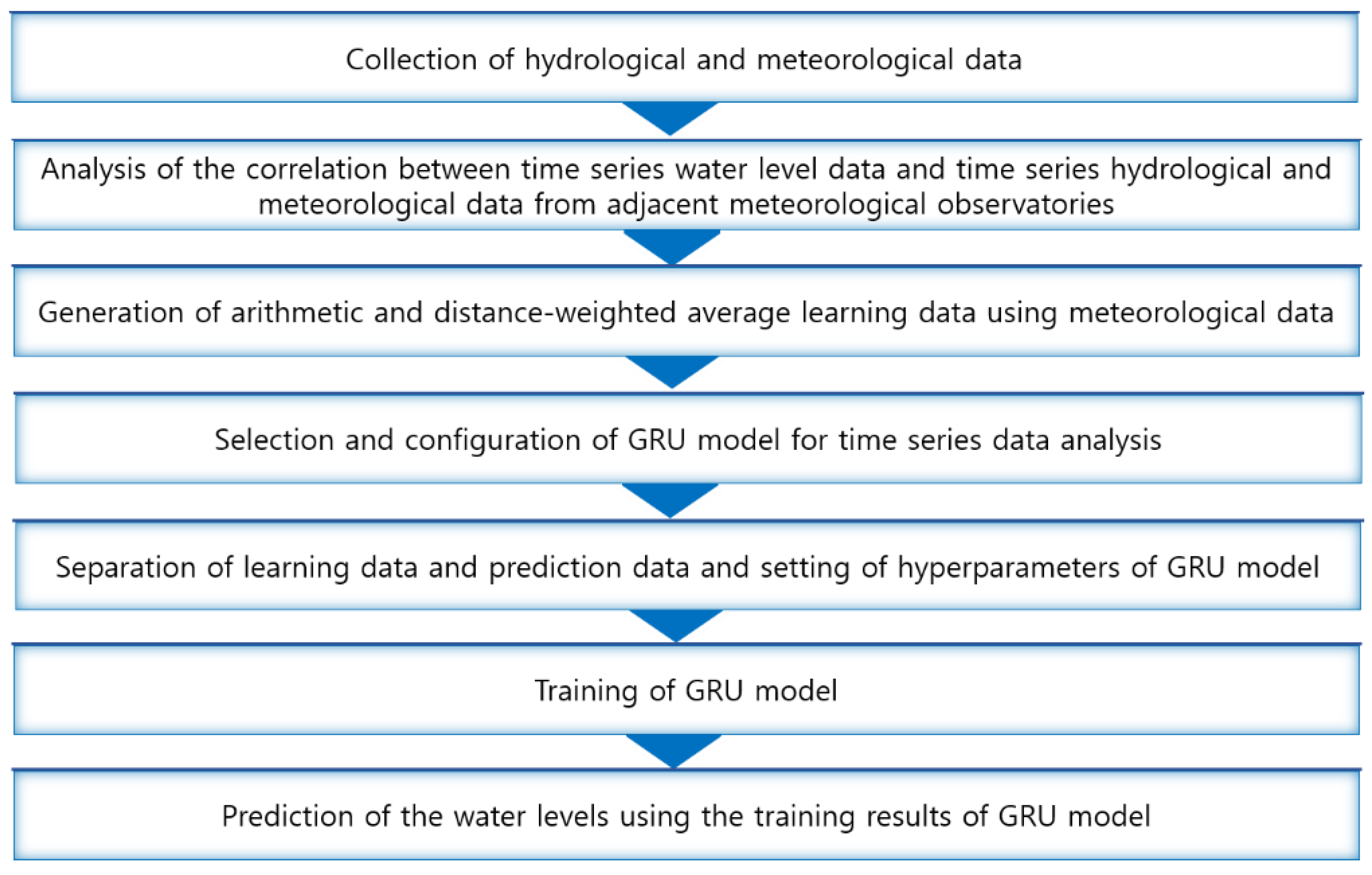
2. Methods
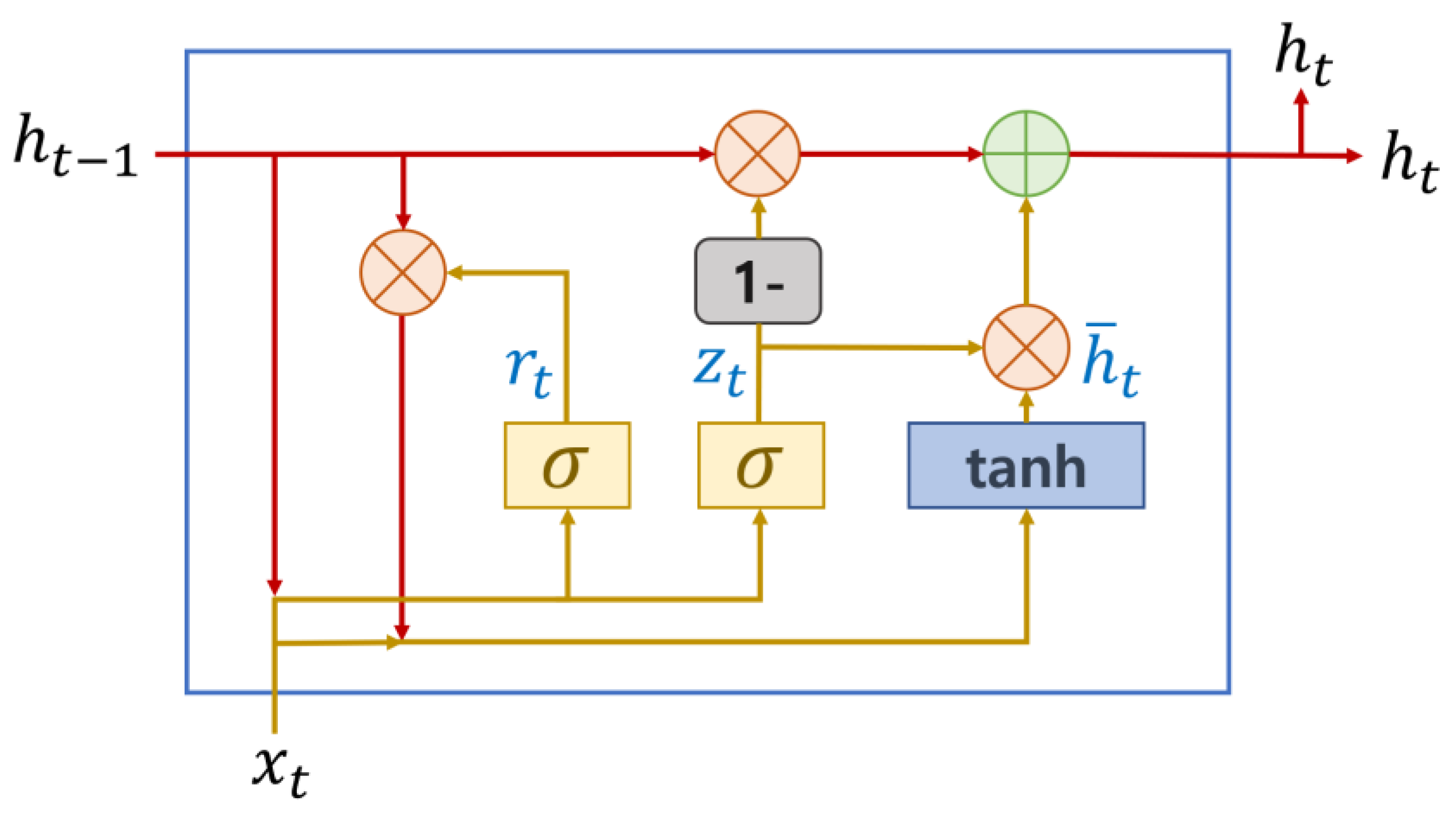
2.1. Gated Recurrent Unit (GRU)
2.2. Model Performance Indicators
- (1)
- Mean Squared Error (MSE)
- (2)
- Root Mean Squared Error (RMSE)
- (3)
- Coefficient of determination (R2)
- (4)
- Nash–Sutcliffe model efficiency coefficient (NSE)
2.3. Application of Models
3. Study Area and Data
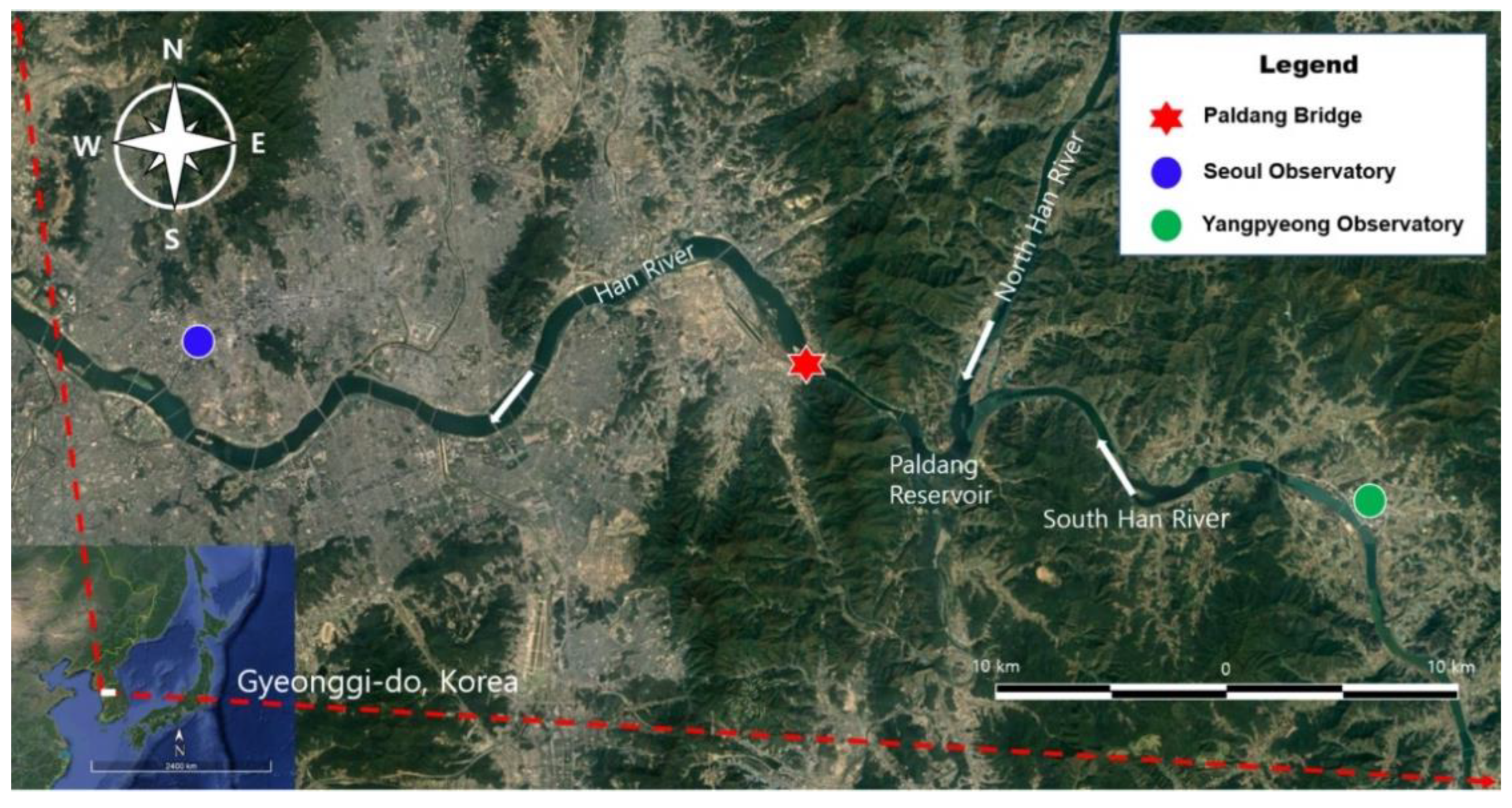
3.1. Study Area
3.2. Hydrologic and Meteorological Data
- (1)
- Daily water level
- (2)
- Hydrological and meteorological data
3.3. Model Composition
- (1)
- Composition of GRU model
- (2)
- Composition of training data in GRU model
4. Results
4.1. Results on Training and Prediction Using Water Levels as Univariate Input Data
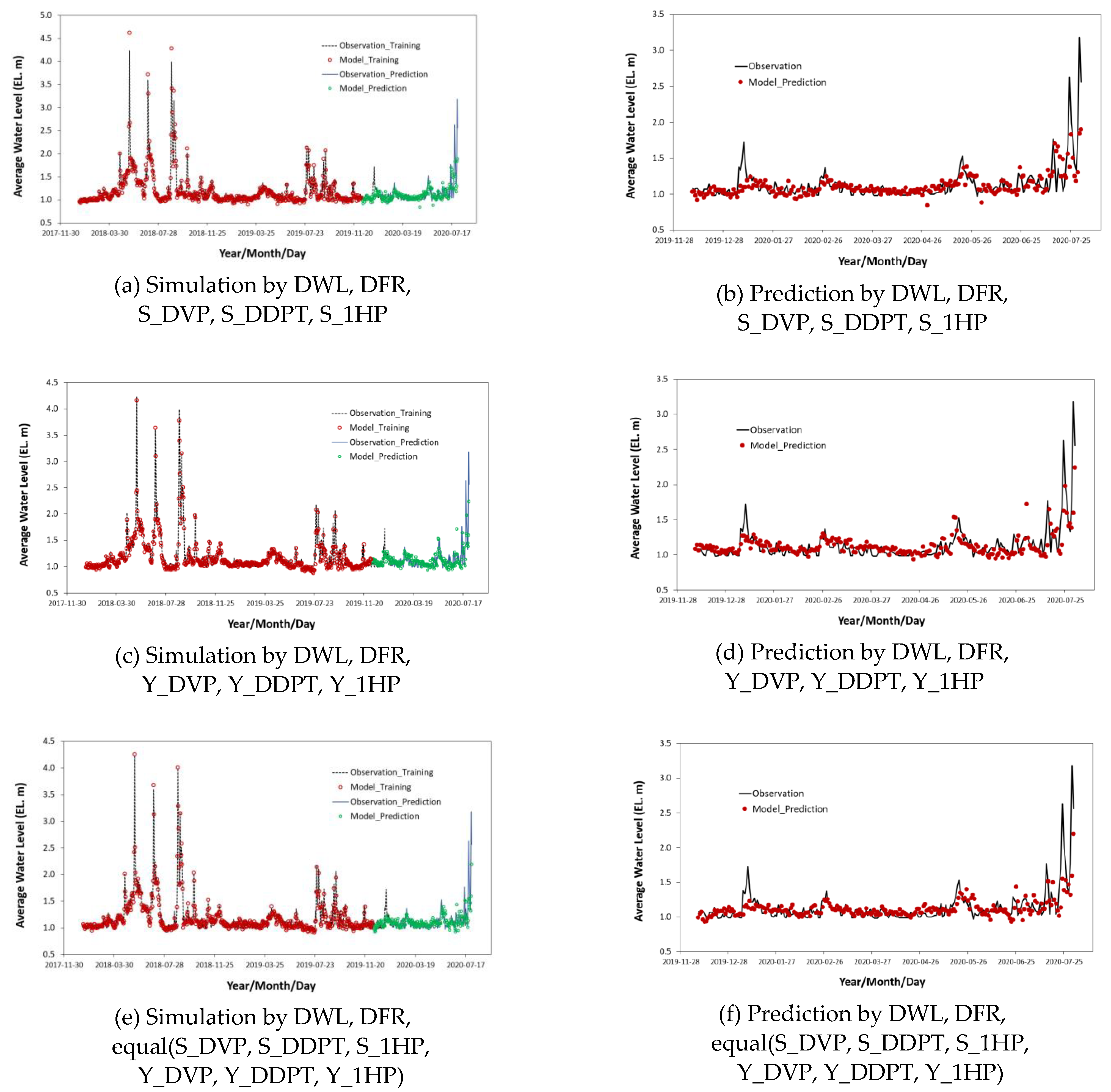
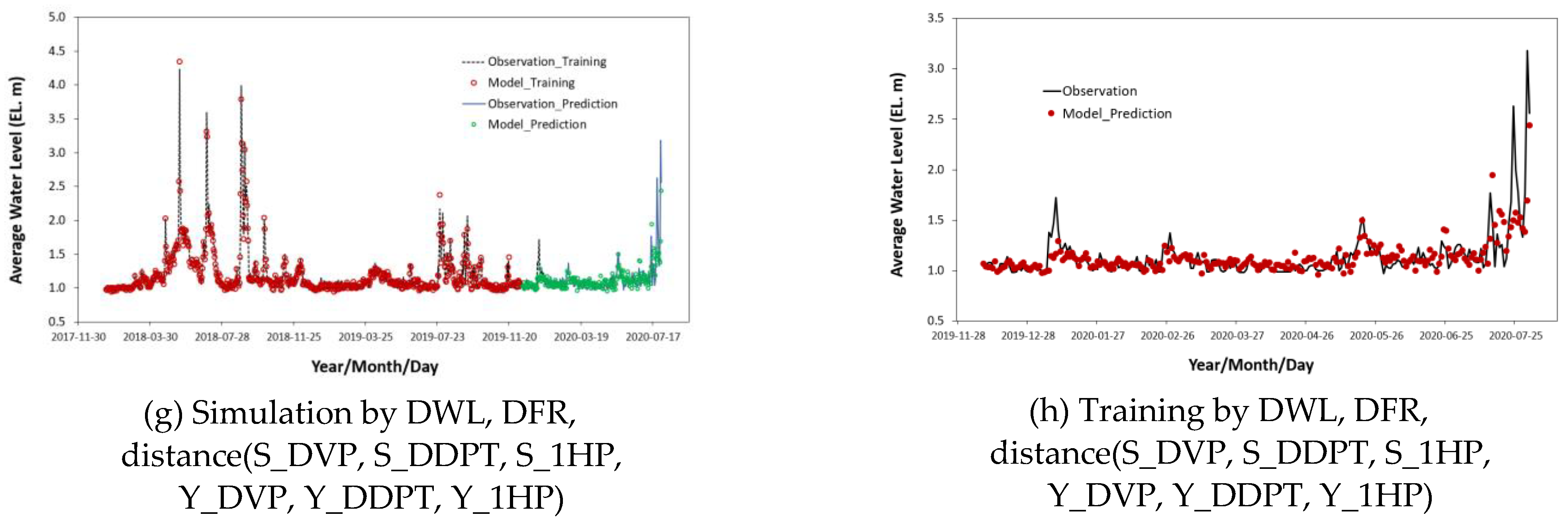
4.2. Results on Training and Prediction Using Water Levels and Multivariate Input Data
5. Discussion
6. Conclusions
Author Contributions
Funding
Institutional Review Board Statement
Informed Consent Statement
Data Availability Statement
Acknowledgments
Conflicts of Interest
References
- Irvine, K.N.; Eberhardt, A.J. Multiplicative, seasonal ARIMA models for Lake Erieand Lake Ontario water levels. JAWRA J. Am. Water Resour. Assoc. 1992, 28, 385–396. [Google Scholar] [CrossRef]
- Tokar, A.S.; Johnson, P.A. Rainfall-runoff modeling using artificial neural networks. J. Hydrol. Eng. ASCE 1999, 4, 232–239. [Google Scholar] [CrossRef]
- Shirmohammadi, B.; Vafakhah, M.; Moosavi, V.; Moghaddamnia, A. Application of several data-driven techniques for predicting groundwater level. Water Resour. Manag. 2013, 27, 419–432. [Google Scholar] [CrossRef]
- Hasebe, M.; Nagayama, Y. Reservoir operation using the neural network and fuzzy systems for dam control and operation support. Adv. Eng. Softw. 2002, 33, 245–260. [Google Scholar] [CrossRef]
- Chang, F.J.; Chang, Y.T. Adaptive neuro-fuzzy inference system for prediction of water level in reservoir. Adv. Water Resour. 2006, 29, 1–10. [Google Scholar] [CrossRef]
- Tran, Q.-K.; Song, S.-K. Water level forecasting based on deep learning: A use case of Trinity River-Texas-the United States. J. KIISE 2017, 44, 607–612. [Google Scholar] [CrossRef]
- Chen, P.-A.; Chang, L.-C.; Chang, F.-J. Reinforced recurrent neural networks for multi-step-ahead flood forecasts. J. Hydrol. 2013, 497, 71–79. [Google Scholar] [CrossRef]
- Adamowski, J.; Chan, H.F. A wavelet neural network conjunction model for groundwater level forecasting. J. Hydrol. 2011, 407, 28–40. [Google Scholar] [CrossRef]
- Partal, T.; Cigizoglu, H.K. Estimation and forecasting of daily suspended sediment data using wavelet-neural networks. J. Hydrol. 2008, 358, 317–331. [Google Scholar] [CrossRef]
- Rajaee, T.; Nourani, V.; Mohammad, Z.K.; Kisi, O. River suspended sediment load prediction: Application of ANN and wavelet conjunction model. J. Hydrol. Eng. 2011, 16, 613–627. [Google Scholar] [CrossRef]
- Adnan, R.; Ruslan, F.A.; Samad, A.M.; Zain, Z.M. Flood Water Level Modelling and Prediction Using Artificial Neural Network: Case Study of Sungai Batu Pahat in Johor. In Proceedings of the 2012 IEEE Control and System Graduate Research Colloquium, Shah Alam, Malaysia, 16–17 July 2012; pp. 22–25. [Google Scholar]
- Kisi, O.; Shiri, J.; Nikoofar, B. Forecasting daily lake levels using artificial intelligence approaches. Comput. Geosci. 2012, 41, 169–180. [Google Scholar] [CrossRef]
- Hipni, A.; El-Shafie, A.; Najah, A.; Karim, O.A.; Hussain, A.; Mukhlisin, M. Daily forecasting of dam water levels: Comparing a support vector machine (SVM) model with adaptive neuro fuzzy inference system (ANFIS). Water Resour. Manag. 2013, 27, 3803–3823. [Google Scholar] [CrossRef]
- Young, C.C.; Liu, W.C.; Hsieh, W.L. Predicting the water level fluctuation in an Alpine Lake using physically based, artificial neural network, and time series forecasting models. Math. Probl. Eng. 2015, 2015, 708204. [Google Scholar] [CrossRef]
- Park, K.; Jung, Y.; Kim, K.; Park, S.K. Determination of deep learning model and optimum length of training data in the river with large fluctuations in flow rates. Water 2020, 12, 3537. [Google Scholar] [CrossRef]
- Guo, F.; Yang, J.; Li, H.; Li, G.; Zhang, Z. A ConvLSTM conjunction model for groundwater level forecasting in a karst aquifer considering connectivity Characteristics. Water 2021, 13, 2759. [Google Scholar] [CrossRef]
- Di Nunno, F.; Granata, F.; Gargano, R.; de Marinis, G. Forecasting of extreme storm tide events using NARX neural network-based models. Atmosphere 2021, 12, 512. [Google Scholar] [CrossRef]
- Di Nunno, F.; de Marinis, G.; Gargano, R.; Granata, F. Tide prediction in the Venice Lagoon using Nonlinear Autoregressive Exogenous (NARX) neural network. Water 2021, 13, 1173. [Google Scholar] [CrossRef]
- Henonin, J.; Russo, B.; Mark, O.; Gourbesville, P. Real-time urban flood forecasting and modelling—A state of the art. J. Hydroinform. 2013, 15, 717–736. [Google Scholar] [CrossRef]
- Jung, S.; Cho, H.; Kim, J.; Lee, G. Prediction of water level in a tidal river using a deep-learning based LSTM model. J. Korea Water Resour. Assoc. 2018, 51, 1207–1216. [Google Scholar]
- Park, K.; Jung, Y.; Seong, Y.; Lee, S. Development of deep learning models to improve the accuracy of water levels time series prediction through multivariate hydrological data. Water 2022, 14, 469. [Google Scholar] [CrossRef]
- Seong, Y.; Park, K.; Jung, Y. Flow rate prediction at Paldang Bridge using deep learning models. J. Korea Water Resour. Assoc. 2022, 55, 565–575. [Google Scholar]
- Moriasi, D.N.; Arnold, J.G.; Van Liew, M.W.; Bingner, R.L.; Harmel, R.D.; Veith, T.L. Model evaluation guidelines for systematic quantification of accuracy in watershed simulations. Soil Water Div. ASABE 2007, 50, 885–900. [Google Scholar]
- Segura-Beltrán, F.; Sanchis-Ibor, C.; Morales-Hernández, M.; González-Sanchis, M.; Bussi, G.; Ortiz, E. Using post-flood surveys and geomorphologic mapping to evaluate hydrological and hydraulic models: The flash flood of the Girona River (Spain) in 2007. J. Hydrol. 2016, 541, 310–329. [Google Scholar] [CrossRef] [Green Version]
- Kastridis, A.; Kirkenidis, C.; Sapountzis, M. An integrated approach of flash flood analysis in ungauged Mediterranean watersheds using post-flood surveys and unmanned aerial vehicles. Hydrol. Process. 2020, 34, 4920–4939. [Google Scholar] [CrossRef]
- Narbondo, S.; Gorgoglione, A.; Crisci, M.; Chreties, C. Enhancing physical similarity approach to predict runoff in ungauged watersheds in sub-tropical regions. Water 2020, 12, 528. [Google Scholar] [CrossRef]
- Chen, H.; Luo, Y.; Potter, C.; Moran, P.J.; Grieneisen, M.L.; Zhang, M. Modeling pesticide diuron loading from the San Joaquin watershed into the Sacramento-San Joaquin Delta using SWAT. Water Res. 2017, 121, 374–385. [Google Scholar] [CrossRef]
- Chiew, F.; Stewardson, M.J.; McMahon, T. Comparison of six rainfall-runoff modelling approaches. J. Hydrol. 1993, 147, 1–36. [Google Scholar] [CrossRef]
- Ministry of Construction and Transportation. Master Plan for River Modification of the Han River Basin; Ministry of Construction and Transportation: Sejong, Republic of Korea, 2002.
- Google Earth. Available online: http://www.google.com/maps (accessed on 1 October 2022).
- Korea Meteorological Administration, National Climate Data Center. Available online: https://data.kma.go.kr (accessed on 1 October 2022).
- Water Resources Management Information System. Available online: http://www.wamis.go.kr (accessed on 1 October 2022).
- Anaconda. Python ver. 3.9.12. Available online: https://www.anaconda.com (accessed on 1 August 2021).
- TensorFlow. TensorFlow ver. 2.10.0. Available online: https://www.tensorflow.org (accessed on 1 August 2021).


| Performance Rating | ||
|---|---|---|
| Very good | ||
| Good | ||
| Satisfactory | ||
| Unsatisfactory |
| Minimum Water Level | Maximum Water Level | Average Water Level | Standard Deviation of Water Level |
|---|---|---|---|
| 0.960 | 4.230 | 1.190 | 0.328 |
| Variable | DWL (EL.m) | DFR (m3/s) | S_1HP (mm) | S_DDPT (°C) | S_DVP (hPa) | Y_1HP (mm) | Y_DDPT (°C) | Y_DVP (hPa) |
|---|---|---|---|---|---|---|---|---|
| DWL (EL.m) | 1.0000 | 0.9735 | 0.2350 | 0.3254 | 0.3328 | 0.3415 | 0.3607 | 0.3809 |
| DFR (m3/s) | 0.9735 | 1.0000 | 0.2512 | 0.2687 | 0.2790 | 0.3281 | 0.3034 | 0.3291 |
| S_1HP (mm) | 0.2350 | 0.2512 | 1.0000 | 0.3047 | 0.3770 | 0.1555 | 0.2402 | 0.2652 |
| S_DDPT (°C) | 0.3254 | 0.2687 | 0.3047 | 1.0000 | 0.9420 | 0.2310 | 0.8407 | 0.8387 |
| S_DVP (hPa) | 0.3328 | 0.2790 | 0.3770 | 0.9420 | 1.0000 | 0.2550 | 0.8228 | 0.8795 |
| Y_1HP (mm) | 0.3415 | 0.3281 | 0.1555 | 0.2310 | 0.2550 | 1.0000 | 0.2796 | 0.3419 |
| Y_DDPT (°C) | 0.3607 | 0.3034 | 0.2402 | 0.8407 | 0.8228 | 0.2796 | 1.0000 | 0.9472 |
| Y_DVP (hPa) | 0.3809 | 0.3291 | 0.2652 | 0.8387 | 0.8795 | 0.3419 | 0.9472 | 1.0000 |
| Activation Function | Input Layer | Hidden Layer 1 | Dropout | Hidden Layer 2 | Dense Layer 1 | Dense Layer 2 |
|---|---|---|---|---|---|---|
| ReLU | GRU | GRU 50 units | 0.25 | GRU 50 units | 25 units | 1 unit |
| Number of Input Variables | Training Data | Prediction Data |
|---|---|---|
| 1 | DWL | DWL |
| 5 | DWL, DFR, S_DVP, S_DDPT, S_1HP | |
| 5 | DWL, DFR, Y_DVP, Y_DDPT, Y_1HP | |
| 8 | DWL, DFR, * equal(S_DVP, S_DDPT, S_1HP, Y_DVP, Y_DDPT, Y_1HP) | |
| 8 | DWL, DFR, ** distance(S_DVP, S_DDPT, S_1HP, Y_DVP, Y_DDPT, Y_1HP) |
| Variable | Computational State | MSE | RMSE | NSE | |
|---|---|---|---|---|---|
| DWL | Training | 7.153 × 10⁻⁶ | 0.0027 | 0.9889 | 0.9870 |
| Prediction | 1.629 × 10⁻⁵ | 0.0040 | 0.5179 | 0.5129 |
| Variables | Computational State | MSE | RMSE | NSE | |
|---|---|---|---|---|---|
| DWL, DFR, S_DVP, S_DDPT, S_1HP | Training | 0.0019 | 0.0437 | 0.9888 | 0.9923 |
| Prediction | 0.0329 | 0.1814 | 0.4660 | 0.5976 | |
| DWL, DFR, Y_DVP, Y_DDPT, Y_1HP | Training | 0.0022 | 0.0470 | 0.9843 | 0.9807 |
| Prediction | 0.0326 | 0.1806 | 0.4896 | 0.5941 | |
| DWL, DFR, * equal(S_DVP, S_DDPT, S_1HP, Y_DVP, Y_DDPT, Y_1HP) | Training | 0.0025 | 0.0497 | 0.9808 | 0.9860 |
| Prediction | 0.0339 | 0.1840 | 0.4676 | 0.6107 | |
| DWL, DFR, ** distance(S_DVP, S_DDPT, S_1HP, Y_DVP, Y_DDPT, Y_1HP) | Training | 0.0018 | 0.0420 | 0.9868 | 0.9868 |
| Prediction | 0.0301 | 0.1734 | 0.5049 | 0.6228 |
Disclaimer/Publisher’s Note: The statements, opinions and data contained in all publications are solely those of the individual author(s) and contributor(s) and not of MDPI and/or the editor(s). MDPI and/or the editor(s) disclaim responsibility for any injury to people or property resulting from any ideas, methods, instructions or products referred to in the content. |
© 2023 by the authors. Licensee MDPI, Basel, Switzerland. This article is an open access article distributed under the terms and conditions of the Creative Commons Attribution (CC BY) license (https://creativecommons.org/licenses/by/4.0/).
Share and Cite
Park, K.; Seong, Y.; Jung, Y.; Youn, I.; Choi, C.K. Development of Water Level Prediction Improvement Method Using Multivariate Time Series Data by GRU Model. Water 2023, 15, 587. https://doi.org/10.3390/w15030587
Park K, Seong Y, Jung Y, Youn I, Choi CK. Development of Water Level Prediction Improvement Method Using Multivariate Time Series Data by GRU Model. Water. 2023; 15(3):587. https://doi.org/10.3390/w15030587
Chicago/Turabian StylePark, Kidoo, Yeongjeong Seong, Younghun Jung, Ilro Youn, and Cheon Kyu Choi. 2023. "Development of Water Level Prediction Improvement Method Using Multivariate Time Series Data by GRU Model" Water 15, no. 3: 587. https://doi.org/10.3390/w15030587