Modelling Runoff from Permeable Pavements: A Link to the Curve Number Method

Abstract

Permeable Pavement (PP) models are valuable tools for studying the implementation of PPs in urban environments. However, the runoff simulated by traditional models such as the Curve Number (CN) is different from that created with PP models, as infiltration is computed differently. However, many investigations compare the runoff created by both models to extract broader conclusions without considering how the two models are related. Hence, this research explores the relation between runoff simulated by one general model, selecting the widespread CN model as a baseline, and the PP model provided in the Storm Water Management Model (SWMM). Correlation was set using the hydrograph created with the CN in a single event as a baseline and obtaining the best pavement permeability value from the PP model by calibration. The influence of storm depth, pavement slope, catchment shape, and PP type was also analysed. Calibration was conducted based on the Nash–Sutcliffe coefficient, but peak and volume performances were also studied. The results show that it is possible to link runoff hydrographs computed with the PP model to those created with the CN method, although that relation is not useful for the entire CN range. That relation is practical for CNs higher than 88 and shall be helpful for urban planners and researchers to compare several pervious/impervious scenarios in urban drainage models more robustly. One direct application is to compare the runoff computed by both models without changing the method that simulates runoff. It shall be enough to change a unique parameter that can be linked to a certain imperviousness by the CN.

1. Introduction

Authorities are increasingly implementing environmentally sustainable solutions in new and existing developments, and urban drainage systems are no exception. In this field, Sustainable Urban Drainage Systems (SUDS) have multiple advantages [1]: they provide energy savings, they mitigate climate change by reducing greenhouse gases, they reduce the urban heat island effect, and they improve community livability by enhancing, among others, aesthetics, recreation possibilities, and biodiverse habitats. In addition, from the stormwater management point of view, SUDS reduce the volume and peak of generated runoff, being recognised as a sustainable strategy to mitigate floods in urban environments [2,3,4,5,6,7,8].

However, both stormwater management and flood mitigation require efficient mathematical models in order to promote sustainable urban environments [3]. However, the increasing number of hydrological model applications in urban environments, together with the greater sustainability challenges, makes it essential to go further in the hydrological processes present in urban areas; hence, these models need to be further explored in order to face existing and new challenges [9].

Regarding stormwater network contribution, runoff is currently the main parameter to characterise the hydrological response of an urban plot [10]. Hence, runoff simulation is a key component of the modelling process, together with the confluence process to the stormwater network. In that regard, hydrologic methods compute catchment runoff based on precipitation excess, with infiltration being the main process that creates precipitation losses. This infiltration can be computed based on several methods, although the relative efficiency of a particular method with respect to others cannot be determined in a definite manner [11].

On the other hand, models integrating SUDS are becoming increasingly common, as they provide an analysis of SUDS’ impact at a catchment scale [12]. These models have been extensively used as optimisation tools for different SUDS configurations, making them an extremely helpful decision resource to explore the hydraulic performance of several SUDS types, study their implementation, and check different setups [3]. Yet, further research is recommended in order to improve modelling techniques for evaluating the performance of SUDS [13].

Permeable Pavements (PP) are one of such SUDS and can be used in walkways, roads, playgrounds, or parking lots, among others [14]. PPs are quite different from other SUDS types, as they ensure a hard surface while providing infiltration and detention capacity, thus reducing additional land requirement for detention facilities and being an alternative for impervious surfaces. This is especially important in urban areas with high land price and highly impervious sites with little or no space for stormwater detention [15,16]. Those implementation factors, together with their environmental benefits, have boosted its implementation [17].

Currently, there are several computational models available to simulate the hydrodynamic behaviour of PPs [14,18], with some of them being integrated into wider urban drainage models [19]. However, as mentioned previously, methods for calculating infiltration in a certain subcatchment are diverse. Moreover, with the implementation of PP models, infiltration can also be computed with the recent, in addition to the traditional, thus overlapping several infiltration methods in the same model. Hence, in a particular urban plot, a traditional method can be selected to compute infiltration, but in the adjoining plot or even in a particular area of the former plot, a PP model may be applied to compute infiltration.

This is a quite common practice in order to study how a certain PP implementation affects the runoff created in a certain urban area. Palla and Gnecco [20] compared runoff peak/volume/delay in a do nothing scenario with several conversion scenarios where PPs were applied. Jato-Espino et al. [21] tested the efficiency of PPs reducing the stormwater volume in the existing drainage system, for which actual/PP scenarios were defined. In addition, Lee et al. [22] created before/after PP situations to check how different climate change scenarios affected to the runoff reduction rate of PPs.

The previous cases are just some examples of how PP efficiency is analysed with a model defining a hypothetical PP scenario. Nevertheless, to analyse the effect of PPs, the same catchment has to be modelled with two different methods, a traditional one, to test current conditions, and the PP model, to test the hypothetical or future scenario. However, can results obtained from different models be directly compared in order to draw certain conclusions? The authors consider that an equivalency or link between models shall be established in order to obtain robust conclusions.

For that purpose, it is common to compare the performance of several models and decide which one is the most suitable for a certain application. In those cases, conclusions are often based on field data. Wilcox et al. [23] compared runoff prediction capabilities, without calibration, for the Soil Conservation Service Curve Number (SCS-CN) and Green–Ampt (GA) models in rural catchments based on real data from six catchments. They concluded that the SCS-CN model, although simpler, performs as well as more complex models. More recently, Ajmal et al. [24] compared the SCS-CN model with a proposed nonlinear model based on one parameter. Proposed nonlinear models, overall, performed better than the SCS-CN model for studied watersheds. In addition, Hu et al. [25] developed a new urban hydrological model that represents nonlinear rainfall–runoff relationships for different urban surfaces and compared it with two commonly used urban hydrological models: the Horton and SCS-CN models. The results showed that their proposed model outperformed the other two models in terms of total runoff and peak flow.

However, measured data are not the only way to produce relevant outcomes: infiltration models can also be compared on a theoretical basis. Zhang and Guo [26] compared the runoff reduction performance of a certain area when infiltration was controlled by the PP model or by the GA model. They found inconsistent results for the PP model for low pavement heights, low drains, and large time steps, so they recommended using the GA method to model PPs. On the other hand, Baiamonte [27] established, assuming constant rainfall intensity, an analytical link between SCS-CN and GA infiltration models, which allowed for an interoperability between both.

Despite its limitations, the SCS-CN method is a popular model compared to those traditional ones because it is simple, predictable, and stable and also because it relies on only one parameter that responds to major properties producing runoff in a watershed [28]. On the other hand, the Storm Water Management Model (SWMM), which implements a PP model, is one of the most popular among researchers due to the diversity of hydrologic and hydraulic computation methods [12]. For instance, the four examples mentioned previously that compared scenarios with and without PP, selected the CN method to control runoff for those subcatchments without PP and the PP model from SWMM to control runoff from PP scenarios. All four compare computed runoff in both subcatchments in order to reach some more general conclusions. However, there is not an obvious link between both models, and hence the comparison cannot be validated.

Consequently, this study explores, on a theoretical basis, the relation between the runoff computed by those two models, the SCS-CN and PP models defined in SWMM, in order to establish, if possible, an equivalency between them, which would be beneficial to derive more consistent outcomes in broader analysis related to the hydraulic benefits of PPs. As SCS-CN relies on one parameter, an equivalent parameter has been selected for the PP model based on a previous sensitivity analysis performed by the authors [29]: pavement permeability. This parameter plays an equivalent role. It is a superficial parameter that controls inflow to the layers below and is also easy to relate and compare against rainfall intensity. More specifically, and from a practical point of view, urban planners, practitioners, and researchers will be able to compare PP implementation runoff scenarios computed on the same model, especially pervious/impervious, by just considering one single parameter, pavement permeability, as this parameter can be linked to a certain CN.

Accordingly, the specific objectives of the article are as follows: (a) explore, on a theoretical basis, the relation between CN and pavement permeability, in order to obtain equivalent runoff hydrographs; (b) analyse the influence of storm depth, pavement slope, catchment shape, and PP type on that relation; and (c) set the conditions in which PP can be used to model runoff equivalent to that modelled by a certain CN.

2. Materials and Methods

This section describes the methodology used in the steps followed during the research process: (1) define the general experimental design, (2) describe the CN method used as a baseline scenario, (3) describe the infiltration provided by both the CN method and the PP module in SWMM, (4) define the model used to obtain the data during the experimental design, and (5) define criteria to compare obtained hydrographs along with the calibration procedure to obtain pavement permeability values.

2.1. Experimental Design

As the objective of this study was to compare runoff created with two different models by linking one parameter from each model, namely, pavement permeability and CN, the study was designed to compute the hydrograph for a certain CN, used as a baseline, and, based on that hydrograph, calibrate the pavement permeability from the PP model. Hence, both models were linked by means of those two parameters: pavement permeability from the PP model and CN from the SCS-CN model. The selected tool to compare both models was SWMM. The model definitions and SWMM implementations are given in Section 2.2 and Section 2.3, while model setup used to compare both methods is given in Section 2.4. The study was also designed to explore how storm depth, pavement slope, catchment shape, and PP type influence that relation.

In order to study the effect of the storm depth, a single design storm was selected, as it is common to rely on them for drainage infrastructure design purposes. Selected return periods were 2, 10, and 100 years, all three with a duration of 6 h [30]. The selected method to define such a storm was the alternating block method [31], based on previously defined IDF curves. Details of the selected IDF curves and defined storm depths are given in Section 2.4.

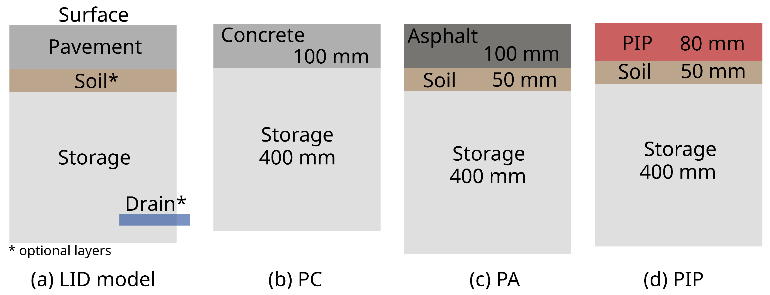
To study the effect of pavement type, three typical permeable cross-sections were selected (see Figure 1): Permeable Concrete (PC), Permeable Asphalt (PA), and Permeable Interlocking Pavers (PIP). Although layer thickness may vary greatly depending on project conditions such as traffic loadings or subgrade bearing capacity, a common layout for urban conditions was defined based on a Spanish standard [32], where 10 cm of asphalt was defined over 40 cm of aggregate. In addition, typical pavement and soil layer thicknesses were selected from the SUDS manual [6]. With this approach, and based on the layout definition provided by SWMM (see Figure 1a), a storage layer of 400 mm depth was defined for all three sections. All but PC were considered with a soil layer of 50 mm. Pavement layer was defined 100 mm thick for PC and PA, but 80 mm for PIP.

To analyse the slope effect, three slopes were selected from the typical range of PPs [33,34]: 1%, 2%, and 6%. As SUDS units are relatively small, the proposed area for the study was 100 m². However, three types of catchment were defined to check the effect of the catchment shape: narrow, squared, and wide catchments. As the defined area was 100 m², shape defining widths were 1 m for the narrow shape, 10 m for the squared shape, and 100 m for the wide shape.

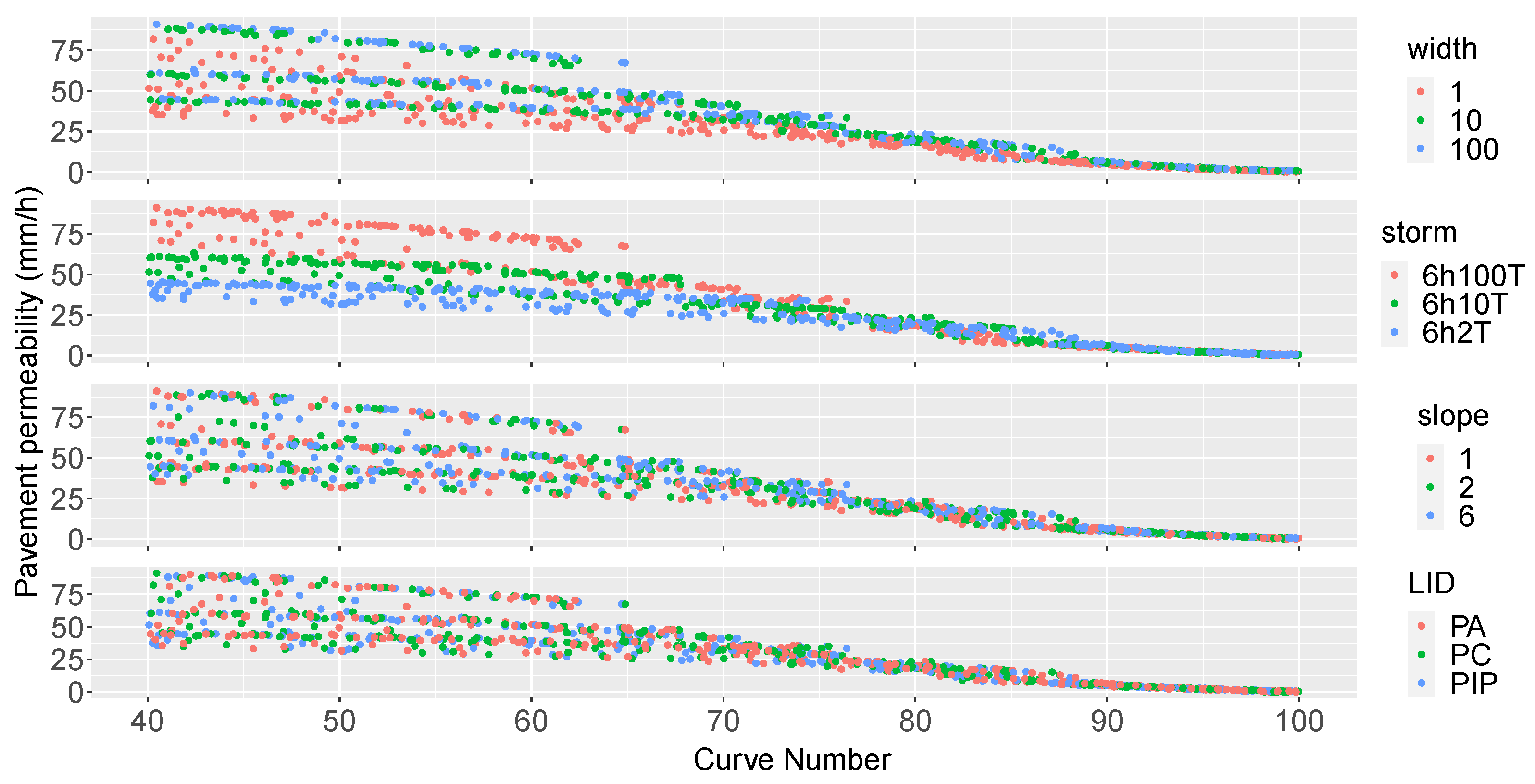
To study the CN effect’s variation, a total of 12 CNs were selected between 40 and 100 for each previously mentioned case. In fact, 12 intervals were selected for that range, and to avoid overlapping points, each of the previous cases was given a random CN from that interval. Considering the three storm depths, three PP types, 3 shapes, 3 slopes, and 12 CNs, for a total of 972 points or relations between CN and pavement permeability, were obtained.

Based on those experimental variables, baseline runoff hydrographs with the SCS-CN method were generated, and their runoff hydrographs were computed. Afterwards, the PP hydrographs were calibrated and, thus, pavement permeability values were obtained. The correlation, obtained for a single event, will later be tested for a continuous event, using continuous 1-year data series.

Data analysis in this study was made with R [35], an open source programming language. Data communication between R and SWMM was carried out with the swmmr package [36]. For model calibration, DE algorithm was used, implemented in the DEoptim package [37].

2.2. Curve Number Method

The CN method from the Soil Conservation Service (SCS), currently the NRCS-CN method, was developed as a method of runoff computation designed for small agricultural watersheds. The method is included in Section 4 of the National Engineering Handbook (NEH-4) published by the SCS, U.S. Department of Agriculture [38]. At first, CN was developed from many experimental watersheds and is now extensively used to calculate direct runoff created by a precipitation event. In spite of being originally intended for agricultural sites, its applicability has also been extended to the urban environment [39].

The SCS-CN method is based on two fundamental hypotheses and the water balance equation, $P=I_a+F+R$, where P is total rainfall, $I_a$ is initial abstraction, F is actual infiltration, and R is the amount of direct surface runoff. The first hypothesis assumes proportional equalities between direct runoff and potential runoff, $R/(P-I_a)$, and actual infiltration and maximum retention, $F/S_{max}$. The term $P-I_a$ represents the effective rainfall or $P_e$, and $S_{max}$ is the maximum potential losses to runoff in $\mathrm{mm}$ or maximum potential difference between effective rainfall and runoff. If that hypothesis and water balance equation are combined, the widely used Equation (1) for runoff (R) computation is obtained, which is dimensionally homogeneous:

$$R=\frac{{(P-I_a)}^2}{(P-I_a)+S_{max}}$$

(1)

The second hypothesis assumes there is some initial abstraction in the beginning of the rainfall, $I_a$, and it is related to potential maximum retention, $S_{max}$, by the factor $\lambda$. Thus, $I_a=\lambda ·S$. Despite the controversy around the value of $\lambda$, the original method gives a median of 0.2 for $\lambda$, as given in Equation (2):

$$I_a=\lambda ·S_{max}=0.2·S_{max}\left[\mathrm{mm}\right]$$

(2)

The value of $S_{max}$ is transformed to CN by an identity, see Equation (3), in order to have a soils/land/cover coefficient with a direct positive relationship to calculated R. The underlying difference between $S_{max}$ and CN is that the former is a dimensional quantity [L], whereas the latter is a non-dimensional quantity and varies conveniently from 0 to 100. Although CN theoretically varies from 0 to 100, values between 40 and 98 are practical design values validated by experience [28]. The original expression gave $S_{max}$ in inches; thus, in metric units, the formula for CN differs from the original [40]:

$$S_{max}=254·\left(\frac{100}{CN}-1\right)\left[\mathrm{mm}\right]$$

(3)

Using the method requires selecting a CN from tables or experience, based on soils land use, hydrologic condition, and initial moisture status. The U.S. Forest Service developed CNs for forested lands, and SCS elaborated woodland runoff CNs. Moreover, CNs for urban lands were built by weighting representative CNs for impervious land types and open spaces in good condition. Current editions of NEH-4 contain a variety of CN tables and charts for an array of additional soils and land uses [40].

2.3. Storm Water Management Model

SWMM is a dynamic rainfall–runoff simulation model used for single-event or long-term (continuous) simulation of runoff quantity and quality from primarily urban areas [41]. Being a distributed model, SWMM divides a urban plot into several subcatchments. As urban areas usually contain a mix of land surfaces, subcatchments can be partitioned into two primary categories: pervious surfaces, allowing infiltration into the soil, and impervious surfaces, over which no infiltration occurs.

A third category can also be added, that corresponding to a SUDS, named Low-Impact Development (LID) control in SWMM, which can be globally defined in the model and, later, included into any subcatchment. It is also possible that the entire subcatchment is occupied by the LID control; in that case, there will not be any pervious or impervious surfaces. This article will just consider two types of surfaces: a pervious area and an LID area completely occupied by PP.

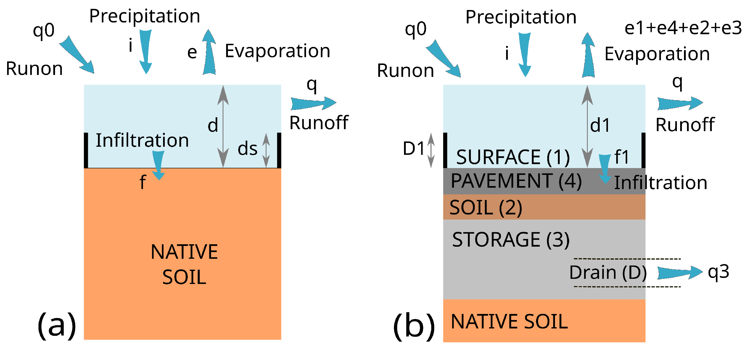
The runoff created in a subcatchment by a rainfall is estimated with a nonlinear reservoir model in SWMM, as shown in Figure 2. Subcatchment inflows are runoff ($q_0$) from other subcatchments and precipitation (i), but the first will not be considered here. Outflows are evaporation (e), infiltration (f), runoff (q), and drain outflow ($q3$). In Figure 2, d or $d_1$ are water level elevations over the infiltration surface; they account for reservoir volume, and $d_s$ or $D_1$ indicate the minimum water level to produce runoff or outflow from the reservoir, respectively.

In order to compute runoff with the SCS-CN method, a standard pervious area was selected, as shown in Figure 2a. The CN method is new to SWMM5 as an alternative to computing infiltration. The model implemented it because most practitioners were familiar with it, but also because there are several tabulated CNs available for numerous soil groups and land uses. The original CN method is a lumped loss method that combines interception, depression storage, and infiltration losses. The method calculates, for a rainfall event, the total rainfall excess. More details about its implementation in SWMM can be found in the hydrology manual [41].

In order to compute runoff with the PP model, an area completely occupied by PP was selected, as shown in Figure 2b. Conceptually, SWMM represents a generic LID unit via multiple horizontal layers, which later are integrated in order to create several LID control types [42]. Specifically, PP is created by combining the following layers (Figure 2): Surface, Pavement, Soil, Storage, and Drain. Two of those layers are optional, Soil and Drain. The model solves a simple mass balance equation for each layer in order to compute hydrological processes into the LID control. Those balances yield the water volume increase or decrease over time by computing the difference between the inflow water flux rate and outflow flux rate [42]. More details about LID units in SWMM can be found in the user’s manual [43].

As shown in Figure 2, the LID model has some differences with a standard subcatchment in SWMM. As mentioned previously, a nonlinear reservoir model is also applied to the LID area, but with some differences. Firstly, we need to consider that inflows (precipitation) are equal in both subcatchments. Secondly, potential evaporation rates are computed in the climatological module of SWMM, and thus, it is equal to both. However, evaporation rates differ because LID areas usually have more water available, as layers below the surface are considered. Hence, the main difference between the two models lies in the infiltration, which is computed differently. That makes computed runoff differ in both areas, even if the evaporation rate remains equal.

The above shows how different computation in a LID area is compared to a pervious area. In the LID area, runoff generation potential relies not just on the native soil properties, but also on the PP layers and their characteristics. For this article, pavement permeability was the selected as the parameter to calibrate runoff, as it is a property of the upper layer and its values are easy to link to an inflow.

2.4. Model Setup

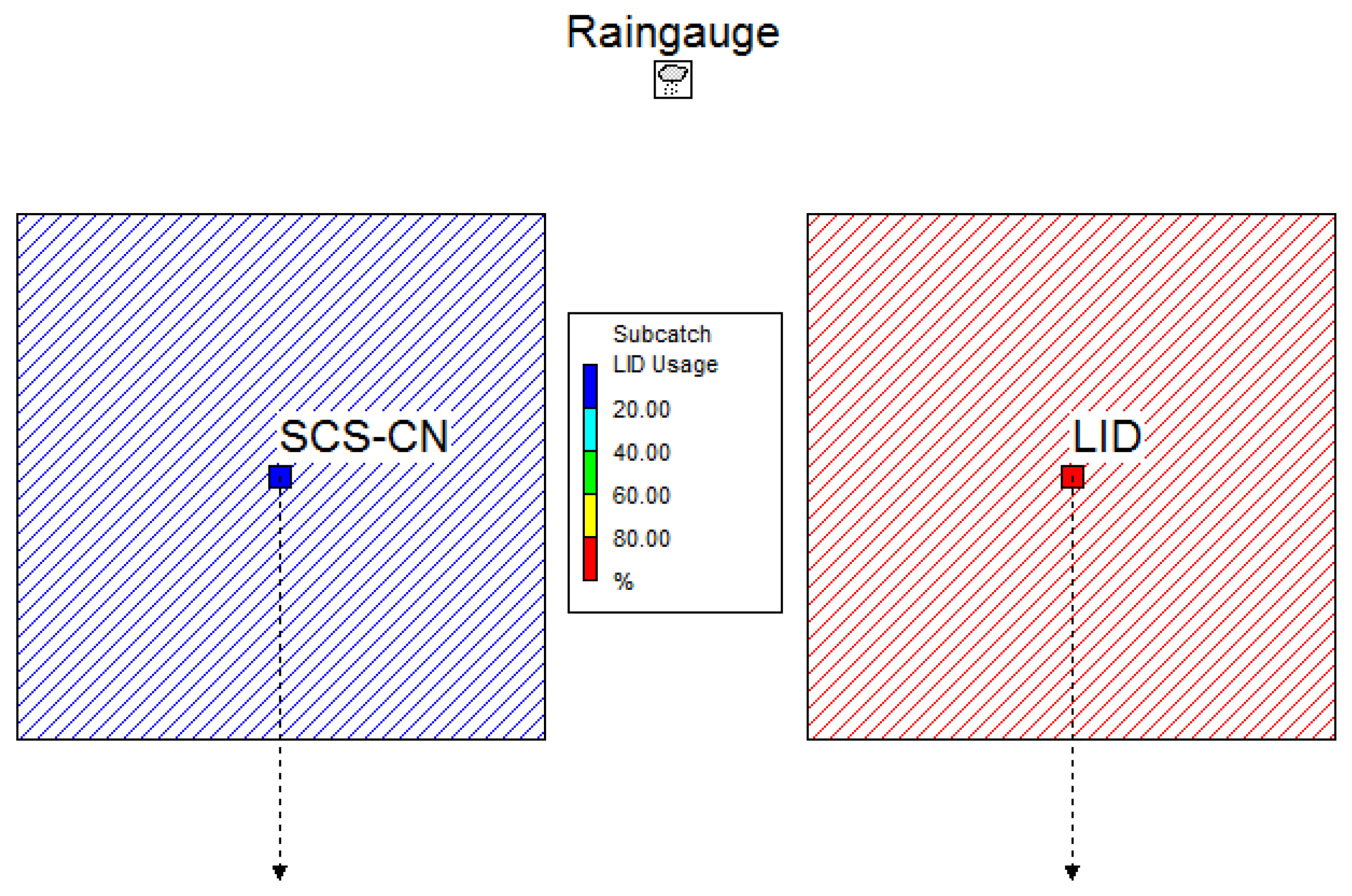
The model setup was designed to compare the performance, in terms of runoff creation capacity, of two different models: the SCS-CN model and the LID model for PPs. To measure and compare runoff hydrographs from two models, two equivalent catchments were created, as shown in Figure 3. The SCS-CN catchment was defined with the general SWMM model and infiltration was calculated with the CN method. The LID catchment was defined as entirely occupied by PP.

SCS-CN catchment characteristics were defined in the catchment properties, while LID properties were set to zero, as they are overwritten by LID properties when modelled as an entirely LID occupied catchment. The used parameters are given in

Table 1. SWMM parameters for subcatchment.

Property	Units	SCS-CN Value	LID Value
Area	ha	0.01	0.01
Width	m	1-10-100	$-{}^{\left(1\right)}$
Slope	%	1-2-6	$-{}^{\left(2\right)}$
% Imperv	%	0	0 ${}^{\left(3\right)}$
N-Perv	Manning n	$0^3$	$-{}^{\left(4\right)}$
Dstore-Perv	mm	1	$-{}^{\left(5\right)}$

⁽¹⁾: defined in the Width for the LID implementation. ⁽²⁾: defined in the Slope for the LID properties. ⁽³⁾: to activate SCS-CN subroutine and prevent runoff delay [41]. ⁽⁴⁾: defined in the Roughness for the LID properties. ⁽⁵⁾: defined in the Berm Height for the LID properties.

. The Manning value for SCS-CN subcatchment was set to zero to avoid any delay in the runoff [41]. Initial abstraction depth was fixed at 1 mm, based on previous studies for urban areas, taking the value for traditional pavements [44].

Although a unique LID control type, PP, was studied, three typical cross-sections were analysed (see Figure 1) to explore if there was any difference in the obtained permeability value. All three types were considered without any drain. Layer properties were identical for all three types, see

Table 2. SWMM parameters for Permeable Pavement type LID controls.

LAYER/Factor	Symbol	Units	PC Value	PP Value	PIP Value
SURFACE
Berm Height	$D_1$	mm	1	1	1
Vegetation Volume Fraction	$1-{\varphi }_1$	-	0	0	0
Roughness	n	Manning n	0.02	0.02	0.02
Slope	S	%	1-2-6	1-2-6	1-2-6
PAVEMENT
Thickness	$D_4$	mm	100	100	80
Void Ratio	${\varphi }_4/(1-{\varphi }_4)$	Voids/Solids	0.25	0.25	0.25
Imperviouss Surf. Frac.	$F_4$	-	0	0	0.9
Permeability	$K_4$	mm/h	*	*	*
SOIL
Thickness	$D_2$	mm	0	50	50
Porosity	${\varphi }_2$	vol. frac.	-	0.45	0.45
Field Capacity	${\theta }_{FC}$	vol. frac.	-	0.1	0.1
Wilting Point	${\theta }_{WP}$	vol. frac.	-	0.05	0.05
Conductivity	$K_{2S}$	mm/h	-	100	100
Conductivity Slope	$HCO$	-	-	50	50
Suction Head	${\psi }_2$	mm	-	50	50
STORAGE
Thickness	$D_3$	mm	400	400	400
Void Ratio	${\varphi }_3/(1-{\varphi }_3)$	Voids/Solids	0.7	0.7	0.7
Seepage Rate	$K_{3S}$	mm/h	10	10	10
DRAIN
Flow Coefficient	$C_{3D}$	-	0	0	0

*: this value is the calibrated parameter.

, but impervious surface fraction was 0.90 for PIP [45]. For all parameters, standard values were used, taken from the SWMM manual [46].

All three PP types were implemented identically into the LID subcatchment, as shown in

Table 3. SWMM parameters for LID implementation into the LID subcatchment.

Property	Units	LID Value
Area of each unit	m${}^2$	100
Number of Units	-	1
Surface Width per Unit	m	1-10-100
% Initially Saturated	%	0
% of Subcatchment Occupied	%	100

.

Climatological data for this study were gathered from the Igeldo weather station (43$°$19${}^{\prime }$0${}^{″}$ N, 2$°$0${}^{\prime }$0${}^{″}$ W) and Miramon weather station (43$°$17${}^{\prime }$20${}^{″}$ N, 1$°$58${}^{\prime }$16${}^{″}$ W), both placed in Donostia/San Sebastián (Spain), which is located in the Bay of Biscay.

The first station was chosen because of its large historical data. In order to study the hydraulic response of the PP, a single event of a 6-hour duration was selected, with a volume of $90.7$ mm for a 100-year return period (named 6hT100), $61.4$ mm for a 10-year return period (named 6hT10), and $43.7$ mm for a 2-year return period (named 6hT2). Those events were obtained from IDF curves created based on Igeldo station data, used to generate a design storm with the alternating block method and considering 15 min time steps.

The second weather station, Miramon, was selected because it had 10 min interval temperature and precipitation data, best suited to perform a continuous or long-term analysis. Thus, in order to test results obtained with the previous single event, data from 2019 were gathered. Annual precipitation is $1593.6$ mm, with 206 dry days (minimum measured values was 0.1 mm). The average temperature for 2019 was 14.2 °C. The Hargreaves method [47] was used to compute evaporation rates based on daily max–min temperatures and the latitude.

For the continuous event, computed time steps were 2:00 min for Wet Weather and 10:00 min for Dry Weather; the reporting time step was 10:00 min. For the single event, the time step for both cases was 1:00 min and the same as the reporting time step.

2.5. Hydrograph Performance and Calibration

Calibration performance was checked by evaluating the Nash–Sutcliffe adimensional coefficient or NSE [48], given by Equation (4) below. Usually, observed and modelled data are compared but, as this research calibrated the parameters for LID to simulate the flows produced by SCS-CN and, therefore, both are modelled, the hydrograph from the SCS-CN area was considered as a baseline scenario and the hydrograph from the LID area as the scenario to be compared. Hence, R is the observed runoff in SCS-CN area, $\overline{R}$ is its average, and $L_i$ is LID area runoff. NSE values range from $-\infty$ to 1, where a value equal to 1 indicates a perfect fit.

$$NSE=1-\frac{{\sum }_{i=1}^N{(R_i-L_i)}^2}{{\sum }_{i=1}^N{(R_i-{\overline{R}}_i)}^2}$$

(4)

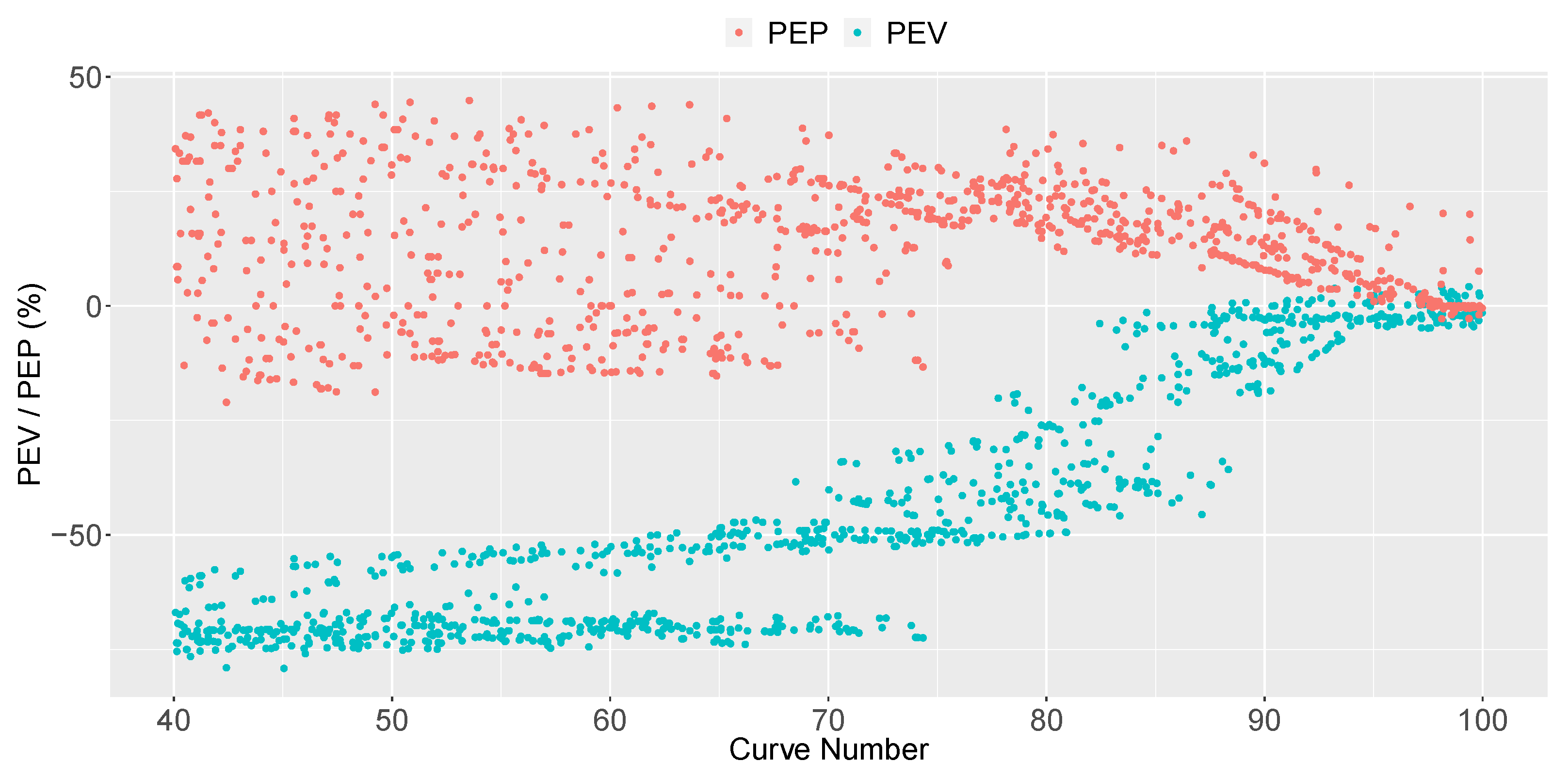
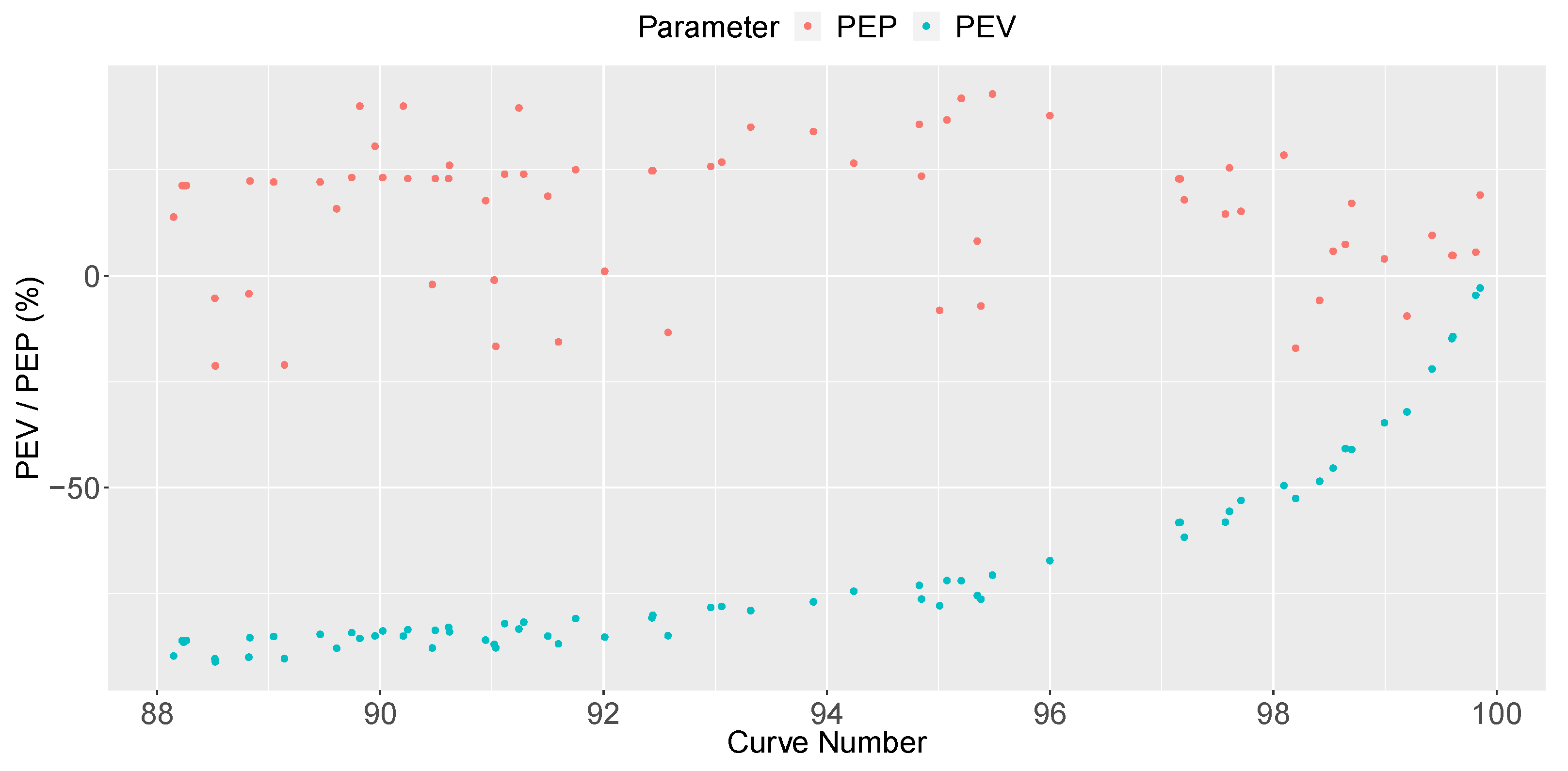
On the other hand, once the calibration parameter was fixed, the resulting runoff hydrographs from both areas were also compared to obtain more information. As it is common to study peak flow and volume for single events [49], percent error in peak (PEP) and percent error in volume (PEV) were analysed, as shown in Equations (5) and (6), the R values being from the SCS-CN subcatchment and the L values from the LID subcatchment:

$$PEP=\frac{L^{peak}-R^{peak}}{R^{peak}}$$

(5)

$$PEV=\frac{L^{volume}-R^{volume}}{R^{volume}}$$

(6)

The calibrated parameter in this study was Pavement Permeability from the Pavement layer of the LID control. The objective function selected for calibration was the NSE defined in Equation (4). For minima searching of the objective function, the Differential Evolution (DE) algorithm was applied, which is one type of meta-heuristic optimization technique based on function evaluation, successfully implemented in multiple areas, as it has prove to be a useful tool for global optimization [50]. In addition, DE is particularly well-suited to find the global optimum of a real-valued function of real-valued parameters, and does not require that the function be either continuous or differentiable [51]. In this study, lower and upper bounds of the parameter to be optimized were (0, 200), and the selected maximum number of iterations (population generation) was 20. These values were validated with a previous test.

3. Results and Discussion

This section presents, firstly, (1) the data obtained after single event calibration: (a) the relation between CN and pavement permeability is presented, which was the main objective of the study; (b) the influence of the selected variables is discussed; and (c) the performance of the calibrated hydrographs is discussed. Secondly, (2) results for a continuous test event are discussed.

3.1. Relation for CN and Pavement Permeability

3.1.1. General Analysis

Obtained pavement permeability values after calibration process for each CN are given in Figure 4. As mentioned in the previous section, those points correspond to three different storm depths, three pavement layouts, three pavement slopes, and three catchment shapes, with 12 CNs for each case; thus, there are 972 points.

The figure shows a clear correlation between both variables linking the two models. As may be expected, the greater the CN, the lower the pavement permeability that generates an equivalent runoff hydrograph. However, the pattern is clearly different for low and high CNs. A visual evaluation reveals that data dispersion is much greater for low CNs than for high CNs. Based on that visual analysis, the authors propose a linear regression differenced by regions, but only the one for high CNs will be considered, given by Equation (7):

$$permeability[\mathrm{mm}/\mathrm{h}]=57-0.57·CNfor88\le CN\le 100$$

(7)

Although the figure does not show how values are influenced for the four considered variables (storm, slope, shape, and type), they are relevant. The influence of those variables will be discussed in the next section. Those variables, along with differences in how the model computes infiltration, vary the response of the PP model.

With regard to the infiltration, the basic difference is how the different methods compute infiltration (see Section 2.3). The infiltration capacity for SCS-CN is not constant: it increases for lower CNs, decreases as storm depth increases, and is higher for narrow catchments. On the other hand, the infiltration capacity of PP relies mainly on the pavement permeability, with a constant value.

It is also important to consider that the SCS-CN method, although varying the infiltration capacity, computes runoff for a wider range of rain intensities if compared to the PP model, which creates runoff for rain intensities higher than pavement permeability. The SCS-CN method computes the partial infiltration of the rain, while the PP model computes runoff over a certain intensity threshold. The rain pattern also plays a role in that infiltration, as intensity varies during storm. Further details will be given in the next two sections.

3.1.2. Influence of Selected Variables

As mentioned before, not all variables have the same influence on pavement permeability. For performing that analysis, Figure 5 has been created, plotting the same figure given in Figure 4 but once for each analysed variable: catchment shape, storm depth, pavement slope, and PP layout.

In regard to catchment shape, characterised by the catchment width, the plot clearly shows that narrow catchments (where the width is equal to 1 m) behave quite differently from the other two catchment types, since the obtained pavement permeability values are lower than for the other two shapes. This is mainly because the time of concentration in the long catchment is considerably higher than the times given by the two other shapes. Hence, water has more time to infiltrate, and thus the equivalent hydrographs in the PP model can be modelled with a lower value of pavement permeability. In addition, pavement permeability values obtained for other considered catchment types are very similar, indicating that only long catchments provide a lower pavement permeability value.

If the storm depth variable is considered, related to the return period, the plot also shows a strong influence on the pavement permeability value. The higher the storm depth, the higher the pavement permeability value that computes an equivalent runoff hydrograph. This pattern may rely on how each model calculates infiltration. In the SCS-CN model, the infiltration increases when precipitation depth increases, while in the PP model, the infiltration capacity is mainly controlled by pavement permeability. That is why pavement permeability has to increase when precipitation depth increases, so that it can increase the infiltration capacity of the PP.

On the contrary, Figure 5 shows how PP layout and pavement slope have no influence on the CN and pavement permeability relation, as those points do not show any pattern. Hence, the following analyses will not consider either one or the other.

3.1.3. Performance of the Equivalent Hydrographs

This section analyses PP runoff hydrographs as compared to the SCS-CN baseline hydrographs. Firstly, some example hydrographs are given in order to better visualize the obtained NSE values. Secondly, the obtained NSE values are presented, as that was the selected criteria to fit the pavement permeability value. Finally, volume and peak performance, PEV and PEP values, are discussed.

Hence, in order to show the relation between SCS-CN baseline hydrographs and calibrated ones, nine hydrogaph pairs are plotted in Figure 6. The first three pairs are given in the first row, and the selected hydrographs are chosen for the same storm and width case, but selecting one with a low CN, one with a medium CN, and another one with a high CN. The second row shows another three pairs of hydrographs, but in this case, the width is constant and similar CNs were selected. The third row has the same storm and similar CNs, varying the width. The effect of those variables will be analysed along with the NSE variable.

Therefore, to check the obtained NSE values after each calibration process, Figure 7 gives 972 NSE values, just grouping the effect for two variables that affect the result, which were previously identified: catchment shape and precipitation depth. Several patterns can be identified from that figure: an improvement in NSE values for higher CNs and also an improvement in those values for higher storm depths and narrower catchments.

Thus, the first thing that Figure 6 clearly shows is that there is an improvement in NSE values while the CN value is increased (see first row of examples in Figure 6). For lower CNs, with high infiltration capacity, the PP can create runoff for the hydrograph peak, but as the infiltration capacity of PP will be higher than other rain intensities, no runoff is created for the rest of the storm. On the contrary, for high CNs, there is almost no infiltration, and thus there is a pavement permeability value that can simulate the baseline hydrograph. This pavement permeability, although constant, will allow similar infiltration to the SCS-CN method.

In that sense, it can be noticed in Figure 7 that the improvement rate is better from a certain CN, different for each combination of storm and shape. That CN is approximately 72 for the 6h2T.100 case (100-year return period and 100 m width or wide catchment). The improvement starts when the infiltration capacity is small enough that the PP can control infiltration with a constant value for a wider range of rain intensities. This depends not only on the considered CN, but also on the selected storm depth and width case.

Something similar happens with the storm depth (see second row of examples in Figure 6). In this case, as the infiltration capacity of the SCS-CN is reduced when storm depth increases, the PP model can accommodate the baseline hydrograph better with just one value of pavement permeability.

With regard to catchment width, the figure also shows that narrow catchments perform differently from square and wide ones (see third row of examples in Figure 6). This is related to the infiltration increase produced by the narrow catchment, where residence time is considerably higher than for wide or squared catchments. For the SCS-CN model, the infiltration increase is smaller in a narrow catchment than the infiltration computed by the PP model in the same type of catchment. As the infiltration capacity is partial in the first and constant in the latter, the increase in infiltration is greater in the PP model for narrow catchments.

It also can be noticed that NSE worsens for some cases, in particular for high CNs and narrow catchments. This is probably due to the same reason mentioned above but, in this case, the increase in the PP model’s infiltration capacity means that the model cannot create as much runoff as the SCS-CN model.

With regard to the peak and volume performance of calibrated hydrographs given in Figure 8, it is clear that there is an improvement for higher CNs, which is related to the obtained NSE values. Overall, the peak values are higher for PP than for the baseline SCS-CN, while volumes are lower for the PP. The obtained peak values are better than the obtained volumes, although both improve considerably for CN values higher than 80. As mentioned before, the PP model is capable of accommodating only the peak value for low and medium CNs. Hence, PEP remains quite constant for all CNs. On the contrary, the PP model cannot accommodate the rest of flow values and, hence, PEV values are worse and only improve when flow rates are fitted not just for the peak, but for a wider range of rain intensities.

Considering both obtained pavement permeabilities and the performance of the calibrated hydrographs, the authors consider that the previously mentioned Equation (7) would give a reasonable equivalent response with the PP model to that obtained with the SCS-CN model. This relation, although not for all CN ranges, would be useful for a wide range of urban covers, mostly impervious (total or partial). However, if that relation is used, it is important to keep in mind that there are some limitations in its performance, as the PP model yields higher peak values and lower volume values.

3.2. Test Case with Continuous Event

This section analyses how pavement permeability values defined using Equation (7) perform when the analysed storm is not a single event but a continuous event. Performance of the PP model is only checked for CN values higher than 88, that is, the range of values which were found to be adequate for considering an equivalent hydrograph with a single event.

The first analysed variable is the NSE, characterising the hydrograph’s performance. The obtained values are given in Figure 9, which shows how CN values are considerably worse than those obtained for a single event. That is, again, due to the differences in model definition. As mentioned in the single event analysis, the infiltration capacity of the PP model is controlled by pavement permeability. If the infiltration capacity obtained by the SCS-CN model was difficult to simulate in a single event, as shown in previous section, it is even more difficult to create an equivalent hydrograph with one unique value if the storm depths are varying, as in the continuous event. Hence, the ability of the PP model to simulate equivalent hydrographs worsens.

The figure also shows that the NSE value improves for high CNs, but this pattern is equivalent to the one obtained for a single event, and the causes are those explained in the preceding section. However, if 0.6 is considered a satisfactory threshold for NSE value, good agreement would be obtained for CNs higher than 96.

If we compare results in terms of volume and peak performance, see Figure 10, we can see that PEP/PEV values also worsen if compared to a single event, although not as much as the NSE. In this continuous event, PEP/PEV values with an error lower than $\pm 50\%$ appear only for CN values higher than 98, while for the single event, that threshold value was around CN 90. This is also explained by the rain pattern and the infiltration method provided by both models. Same as in the single event, peak values perform better than volumes in the continuous event.

Hence, this continuous test case shows that permeability values obtained with Equation (7) are only acceptable for very impervious surfaces or very high CNs, over 96 if we consider obtained NSE values. However, if peak and volume performance are considered, the relation would only be valid for impervious surfaces, that is, for CNs higher than 99.

4. Conclusions

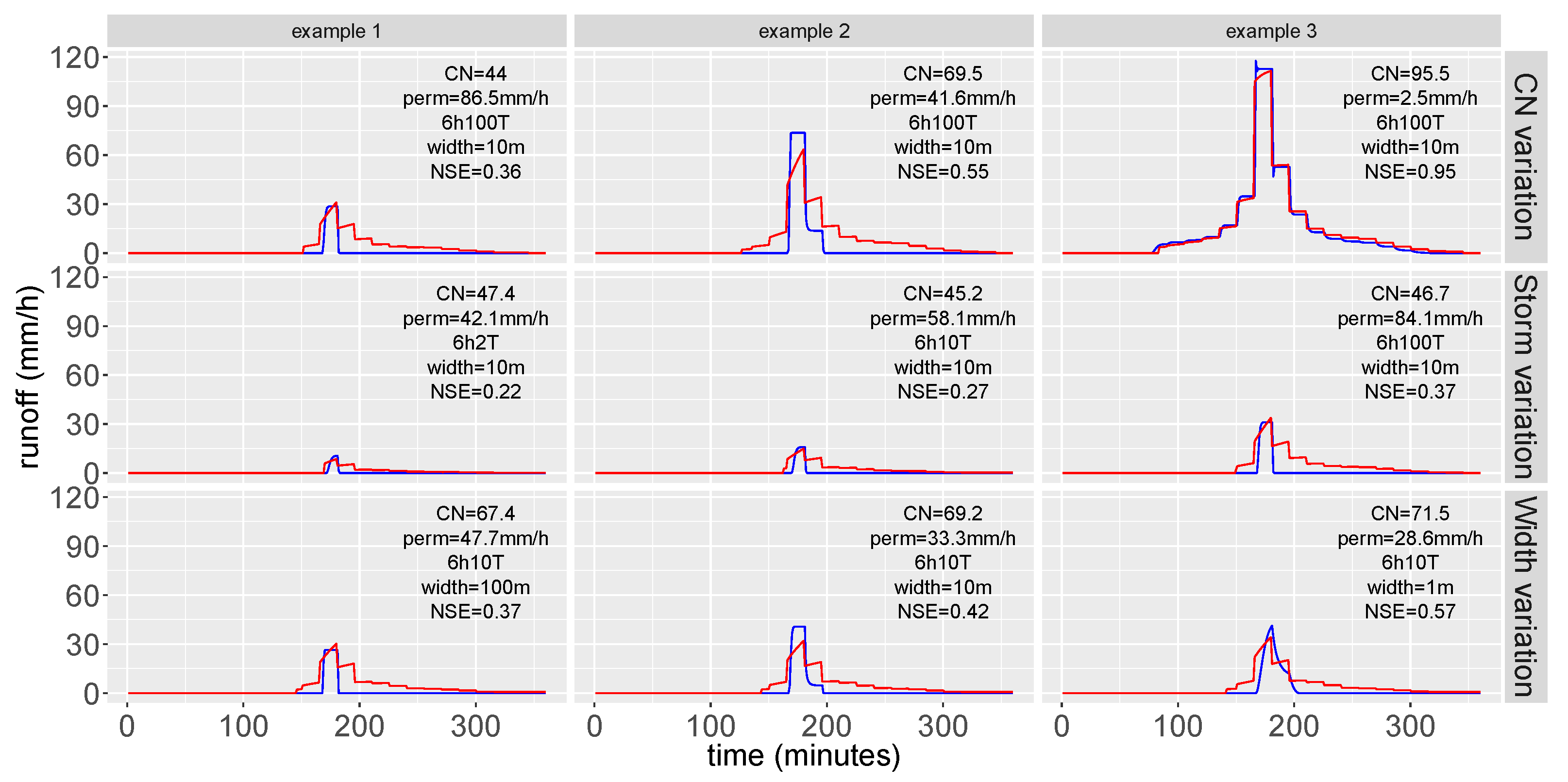
This study compares the hydraulic performance of the PP model given in SWMM and the widespread CN model by linking one parameter from each model: pavement permeability from the first and CN from the latter. The comparison has been performed with SWMM, analysing the influence of several variables involved in the PP’s design: storm depth, pavement layout, catchment shape, and pavement slope. However, it should be noted that the research was not designed to test or compare the performance of any of the mentioned models separately; the aim of the research was to link both models numerically, based on a theoretical comparison.

The article explores how different the models are and, thus, how the runoff modelled in each case differs from the other, as infiltration computations varies. Because of that disparity, the article demonstrates that we cannot consider an equivalence between the runoff hydrographs for pervious surfaces or low CNs. In addition, the article shows that catchment width and storm depth considerably influence the infiltration process, and thus the equivalency between models is significantly influenced by these variables. The article also shows that pavement slope and PP layout do not have impact on that equivalency.

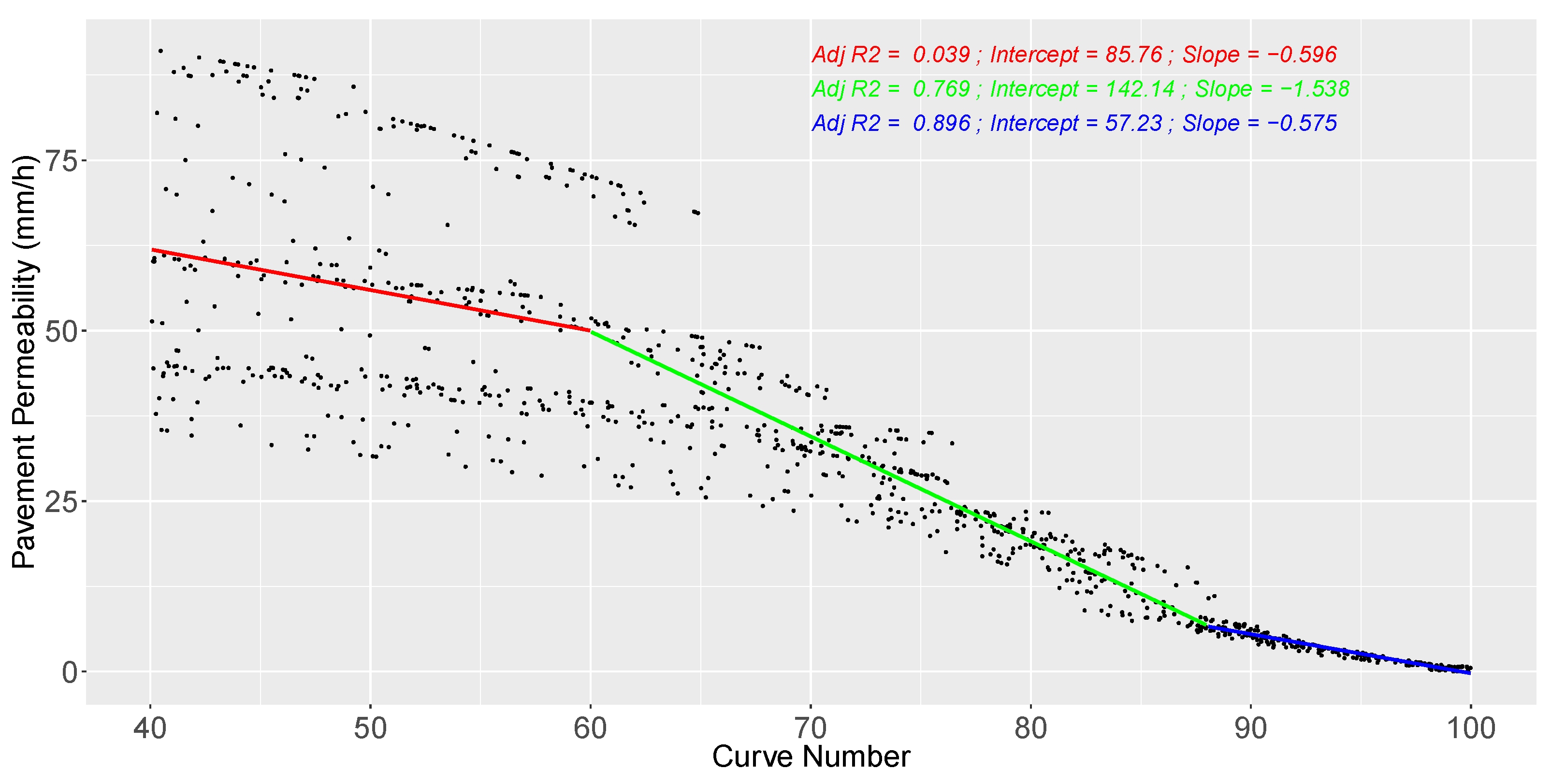
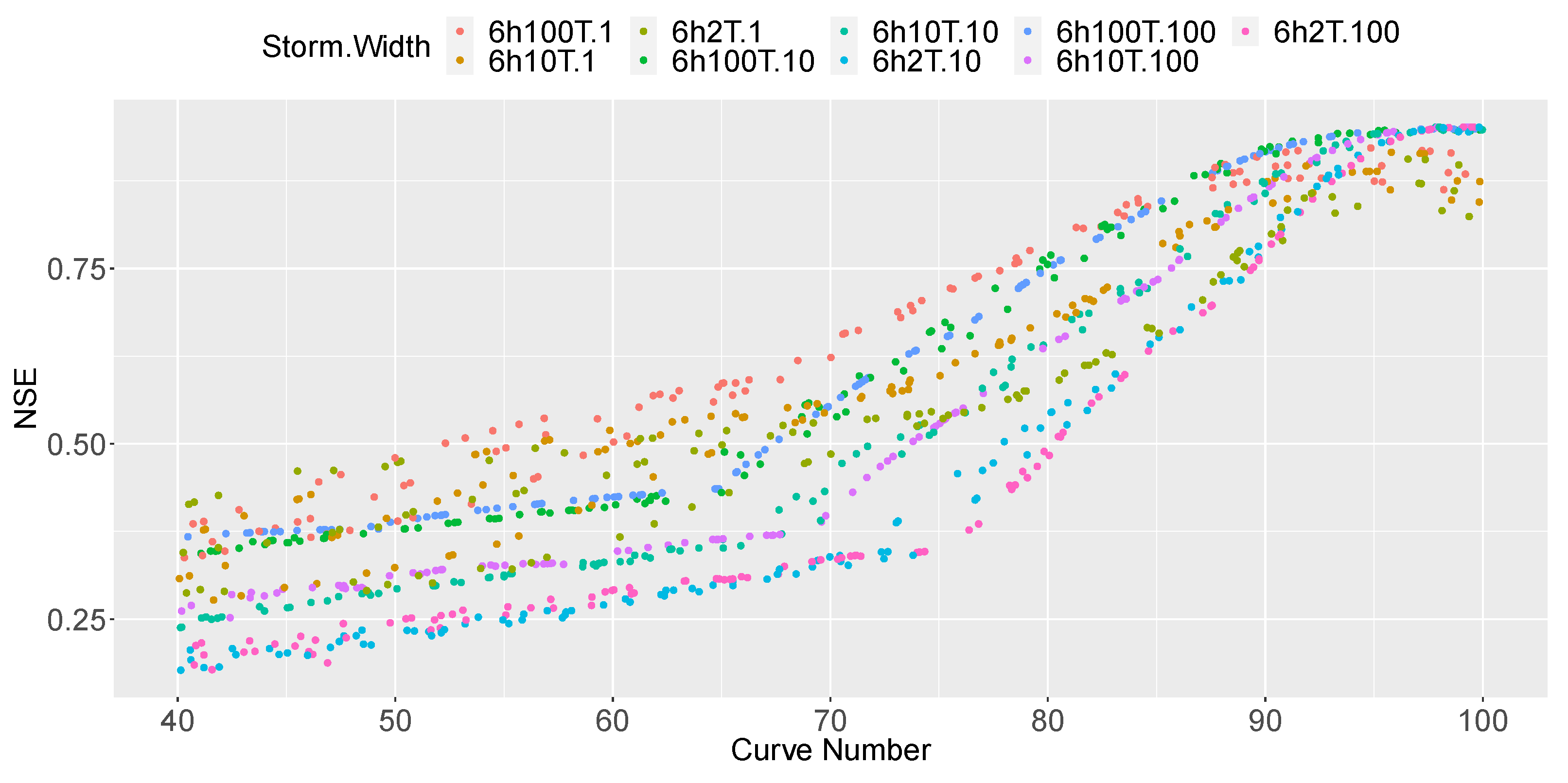
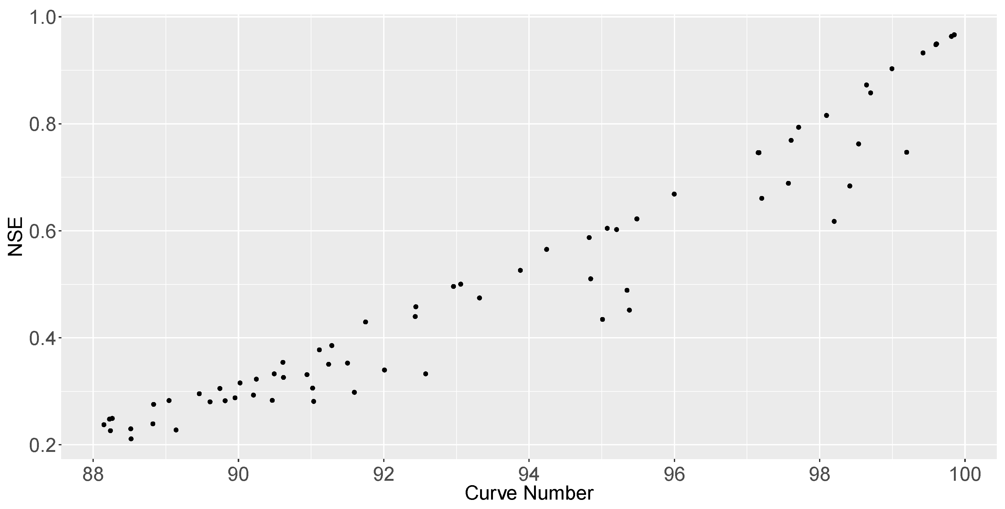
However, this study shows that it is possible to generate runoff hydrographs with the PP model given in SWMM equivalent to those created with the SCS-CN method in some cases. In fact, the article gives a relation between a certain CN and the pavement permeability that creates an equivalent runoff hydrograph: $permeability$ [mm/h] = $57-0.57·CN$. This relation would be valid for single events when CNs are higher than 88 and would not be influenced by the PP layout, catchment shape, storm depth, nor the pavement slope. Equivalent hydrographs would have an NSE higher than 0.60, and peak/volume performances would be in the range of $\pm 50\%$.

This was the primary goal of the article: to find an equivalency for both methods. That relation can be useful, when modelling, to compare runoff created in a certain catchment with and without PP, that is, to analyse the influence of a particular PP design based on runoff data gathered with the same model, providing more robust conclusions in broader studies. Although the conducted analysis makes the relation valid just for the PP model definition given in SWMM, it may be useful for any other PP model, or even SUDS, where infiltration is controlled by a similar surface parameter equivalent to pavement permeability; however, further studies are required.

From a purely practical perspective, it would not be necessary to change the model to check those two scenarios, as PP could also serve as an impervious surface. In addition, PP layouts are defined once in SWMM and can be implemented in several catchments. Thus, it would be enough to change one unique parameter, namely pavement permeability, just once to change the catchment response: for example, from a completely impervious surface type to a catchment with a PP, no matter how many PPs are implemented in the model.

The article also shows that the mentioned equivalency is not valid if a continuous event is modelled. In that case, the PP is much worse at obtaining a hydrograph similar to that created by the SCS-CN. Hence, a continuous event shall not be modelled using the mentioned equivalency if it does not have a CN higher than 98. In this case, the selected test event yields NSE values higher than 0.60, peak errors lower than $25\%$, and volume errors higher than $-50\%$. However, the above-mentioned benefits remain valid: the same model can be used to test PP implementation.

Further research is recommended for other LID types, where the permeable pavement parameter does not exist and surface permeability is controlled by other parameters. Thus, it would be interesting to further study what the relation would look like for other types of SUDS, as those are also studied when implementing SUDS in urban environments. It also would be interesting to investigate if LID control implementation in SWMM may become simpler, as many parameters need to be changed in order to modify a catchment completely occupied by an LID to another one with a different infiltration model. Further studies are also recommended to check the links between SUDS and other models, such as the Rational one, which is also common among practitioners.

In summary, the article compares two widespread models used in urban environments that simulate runoff hydrographs and specifies under which conditions equivalent hydrographs can be obtained. Consequently, the article is expected to be useful for practitioners analysing how the implementation of certain PPs affects the runoff created in one or several areas.

References

1. Charlesworth, S.M. A review of the adaptation and mitigation of global climate change using sustainable drainage in cities. J. Water Clim. Chang. 2010, 1, 165–180. [Google Scholar] [CrossRef]
2. Ciriminna, D.; Ferreri, G.B.; Noto, L.V.; Celauro, C. Numerical Comparison of the Hydrological Response of Different Permeable Pavements in Urban Area. Sustainability 2022, 14, 5704. [Google Scholar] [CrossRef]
3. Qi, W.; Ma, C.; Xu, H.; Chen, Z.; Zhao, K.; Han, H. A review on applications of urban flood models in flood mitigation strategies. Nat. Hazards 2021, 108, 31–62. [Google Scholar] [CrossRef]
4. Liu, T.; Lawluvy, Y.; Shi, Y.; Yap, P.S. Low Impact Development (LID) Practices: A Review on Recent Developments, Challenges and Prospects. Water Air Soil Pollut. 2021, 232, 344. [Google Scholar] [CrossRef]
5. Huang, C.L.; Hsu, N.S.; Liu, H.J.; Huang, Y.H. Optimization of Low Impact Development Layout Designs for Megacity Flood Mitigation. J. Hydrol. 2018, 564, 542–558. [Google Scholar] [CrossRef]
6. Woods Ballard, B.; Wilson, S.; Udale-Clarke, H.; Illman, S.; Ashley, R.; Kellagher, R. The SUDS Manual; Ciria: London, UK, 2015; p. 937. [Google Scholar]
7. Fletcher, T.D.; Shuster, W.; Hunt, W.F.; Ashley, R.; Butler, D.; Arthur, S.; Trowsdale, S.; Barraud, S.; Semadeni-Davies, A.; Bertrand-Krajewski, J.L.; et al. SUDS, LID, BMPs, WSUD and More—The Evolution and Application of Terminology Surrounding Urban Drainage. Urban Water J. 2015, 12, 525–542. [Google Scholar] [CrossRef]
8. Fletcher, T.D.; Andrieu, H.; Hamel, P. Understanding, management and modelling of urban hydrology and its consequences for receiving waters: A state of the art. Adv. Water Resour. 2013, 51, 261–279. [Google Scholar] [CrossRef]
9. Salvadore, E.; Bronders, J.; Batelaan, O. Hydrological modelling of urbanized catchments: A review and future directions. J. Hydrol. 2015, 529, 62–81. [Google Scholar] [CrossRef]
10. Ahiablame, L.M.; Shakya, R. Modeling flood reduction effects of low impact development at a watershed scale. J. Environ. Manag. 2016, 171, 81–91. [Google Scholar] [CrossRef]
11. Luo, P.; Luo, M.; Li, F.; Qi, X.; Huo, A.; Wang, Z.; He, B.; Takara, K.; Nover, D.; Wang, Y. Urban flood numerical simulation: Research, methods and future perspectives. Environ. Model. Softw. 2022, 156, 105478. [Google Scholar] [CrossRef]
12. Kaykhosravi, S.; Khan, U.T.; Jadidi, A. A comprehensive review of low impact development models for research, conceptual, preliminary and detailed design applications. Water 2018, 10, 1541. [Google Scholar] [CrossRef] [Green Version]
13. Eckart, K.; McPhee, Z.; Bolisetti, T. Performance and Implementation of Low Impact Development—A Review. Sci. Total Environ. 2017, 607, 413–432. [Google Scholar] [CrossRef]
14. Kuruppu, U.; Rahman, A.; Rahman, M.A. Permeable pavement as a stormwater best management practice: A review and discussion. Environ. Earth Sci. 2019, 78, 1–20. [Google Scholar] [CrossRef]
15. Zhu, Y.; Li, H.; Liang, X.; Yang, B.; Zhang, X.; Mahmud, S.; Zhang, X.; Zhuang, L.; Zhu, Y. Permeable Pavement Design Framework for Urban Stormwater Management Considering Multiple Criteria and Uncertainty. J. Clean. Prod. 2021, 293, 126114. [Google Scholar] [CrossRef]
16. Li, H.; Kayhanian, M.; Harvey, J.T. Comparative field permeability measurement of permeable pavements using ASTM C1701 and NCAT permeameter methods. J. Environ. Manag. 2013, 118, 144–152. [Google Scholar] [CrossRef] [PubMed]
17. Chandrappa, A.K.; Biligiri, K.P. Pervious Concrete as a Sustainable Pavement Material—Research Findings and Future Prospects: A State-of-the-Art Review. Constr. Build. Mater. 2016, 111, 262–274. [Google Scholar] [CrossRef]
18. Elliott, A.H.; Trowsdale, S.A. A Review of Models for Low Impact Urban Stormwater Drainage. Environ. Model. Softw. 2007, 22, 394–405. [Google Scholar] [CrossRef]
19. Bach, P.M.; Rauch, W.; Mikkelsen, P.S.; McCarthy, D.T.; Deletic, A. A critical review of integrated urban water modelling—Urban drainage and beyond. Environ. Model. Softw. 2014, 54, 88–107. [Google Scholar] [CrossRef]
20. Palla, A.; Gnecco, I. Hydrologic modeling of Low Impact Development systems at the urban catchment scale. J. Hydrol. 2015, 528, 361–368. [Google Scholar] [CrossRef]
21. Jato-Espino, D.; Charlesworth, S.M.; Bayon, J.R.; Warwick, F. Rainfall-Runoff Simulations to Assess the Potential of Suds for Mitigating Flooding in Highly Urbanized Catchments. Int. J. Environ. Res. Public Health 2016, 13, 149. [Google Scholar] [CrossRef]
22. Lee, S.; Kim, D.; Maeng, S.; Azam, M.; Lee, B. Runoff Reduction Effects at Installation of LID Facilities under Different Climate Change Scenarios. Water 2022, 14, 1301. [Google Scholar] [CrossRef]
23. Wilcox, B.P.; Rawls, W.J.; Brakensiek, D.L.; Wight, J.R. Predicting Runoff from Rangeland Catchments: A Comparison of Two Models. Water Resour. Res. 1990, 26, 2401–2410. [Google Scholar] [CrossRef]
24. Ajmal, M.; Waseem, M.; Ahn, J.H.; Kim, T.W. Improved Runoff Estimation Using Event-Based Rainfall-Runoff Models. Water Resour. Manag. 2015, 29, 1995–2010. [Google Scholar] [CrossRef]
25. Hu, C.; Xia, J.; She, D.; Song, Z.; Zhang, Y.; Hong, S. A New Urban Hydrological Model Considering Various Land Covers for Flood Simulation. J. Hydrol. 2021, 603, 126833. [Google Scholar] [CrossRef]
26. Zhang, S.; Guo, Y. SWMM simulation of the Storm Water volume control performance of permeable pavement systems. J. Hydrol. Eng. 2015, 20, 06014010. [Google Scholar] [CrossRef]
27. Baiamonte, G. SCS Curve Number and Green-Ampt Infiltration Models. J. Hydrol. Eng. 2019, 24, 04019034. [Google Scholar] [CrossRef]
28. Ponce, V.M.; Hawkins, R.H. Runoff curve number: Has it reached maturity? J. Hydrol. Eng. 1996, 1, 11–19. [Google Scholar] [CrossRef]
29. Madrazo-Uribeetxebarria, E.; Garmendia Antín, M.; Almandoz Berrondo, J.; Andrés-Doménech, I. Sensitivity analysis of permeable pavement hydrological modelling in the Storm Water Management Model. J. Hydrol. 2021, 600, 126525. [Google Scholar] [CrossRef]
30. Watt, E.; Marsalek, J. Critical review of the evolution of the design storm event concept. Can. J. Civ. Eng. 2013, 40, 105–113. [Google Scholar] [CrossRef]
31. Te Chow, V.; Maidment, D.R.; Mays, L.W. Applied Hydrology; McGraw-Hill: New York, NY, USA, 1988. [Google Scholar]
32. MOPU. Norma 6.1-IC-Secciones de Firme; Technical Report; Ministerio de Obras Públicas y Urbanismo (MOPU): Madrid, Spain, 1986. [Google Scholar]
33. CALTRANS. Pervious Pavement Design Guidance; Technical Report; California Department of Transportation (CALTRANS): Sacramento, CA, USA, 2013.
34. CASQA. Stormwater Best Management Practice Handbook; Technical Report; California Stormwater Quality Association (CASQA): Sacramento, CA, USA, 2003. [Google Scholar]
35. R Core Team. R: A Language and Environment for Statistical Computing; R Foundation for Statistical Computing: Vienna, Austria, 2020. [Google Scholar]
36. Leutnant, D.; Döring, A.; Uhl, M. swmmr—An R package to interface SWMM. Urban Water J. 2019, 16, 68–76. [Google Scholar] [CrossRef]
37. Ardia, D.; Mullen, K.M.; Peterson, B.G.; Ulrich, J. DEoptim: Differential Evolution in R. Version 2.2-5. 2020. Available online: https://cran.r-project.org/web/packages/DEoptim/DEoptim.pdf (accessed on 1 March 2021).
38. SCS. Hydrology, National Engineering Handbook; USDA: Washington DC, USA, 1956.
39. Balbastre-Soldevila, R.; García-Bartual, R.; Andrés-Doménech, I. A Comparison of Design Storms for Urban Drainage System Applications. Water 2019, 11, 757. [Google Scholar] [CrossRef] [Green Version]
40. Hawkins, R.H.; Ward, T.J.; Woodward, D.E.; Van Mullem, J.A. Curve Number Hydrology: State of the Practice; Technical Report; Environmental and Water Resources Institute (EWRI) of the American Society of Civil Engineers: Reston, VA, USA, 2009. [Google Scholar] [CrossRef]
41. Rossman, L.A.; Huber, W.C. Volume I—Hydrology. In Storm Water Management Model Reference Manual; US EPA Office of Research and Development: Washington, DC, USA, 2016. [Google Scholar]
42. Rossman, L.A. Modeling low impact development alternatives with SWMM. J. Water Manag. Model. 2010, 11, 167–182. [Google Scholar] [CrossRef] [Green Version]
43. Rossman, L. Storm Water Management Model User’s Manual Version 5.1; US EPA Office of Research and Development: Washington, DC, USA, 2015.
44. Rammal, M.; Berthier, E. Runoff Losses on Urban Surfaces during Frequent Rainfall Events: A Review of Observations and Modeling Attempts. Water 2020, 12, 2777. [Google Scholar] [CrossRef]
45. Mullaney, J.; Lucke, T. Practical Review of Pervious Pavement Designs. Clean Soil Air Water 2014, 42, 111–124. [Google Scholar] [CrossRef]
46. Rossman, L.A.; Huber, W.C. Volume III—Water Quality. In Storm Water Management Model Reference Manual; US EPA Office of Research and Development: Washington, DC, USA, 2016. [Google Scholar]
47. Hargreaves, G.H.; Samani, Z.A. Reference crop evapotranspiration from temperature. Appl. Eng. Agric. 1985, 1, 96–99. [Google Scholar] [CrossRef]
48. Nash, J.E.; Sutcliffe, J.V. River flow forecasting through conceptual models part I—A discussion of principles. J. Hydrol. 1970, 10, 282–290. [Google Scholar] [CrossRef]
49. Dietz, M.E. Low impact development practices: A review of current research and recommendations for future directions. Water Air Soil Pollut. 2007, 186, 351–363. [Google Scholar] [CrossRef]
50. Pant, M.; Zaheer, H.; Garcia-Hernandez, L.; Abraham, A. Differential Evolution: A review of more than two decades of research. Eng. Appl. Artif. Intell. 2020, 90, 103479. [Google Scholar] [CrossRef]
51. Mullen, K.; Ardia, D.; Gil, D.; Windover, D.; Cline, J. DEoptim: An R Package for Global Optimization by Differential Evolution. J. Stat. Softw. 2011, 40, 1–26. [Google Scholar] [CrossRef]
Figure 1. PP layouts for (a) general SWMM model, and tested (b) PC, (c) PA, and (d) PIP.
Water 15 00160 g001
Figure 2. Non-linear reservoir models for (a) a pervious area and (b) an LID area.
Water 15 00160 g002
Figure 3. Defined catchments: completely pervious (blue) and 100% LID occupied (red).
Water 15 00160 g003
Figure 4. Pavement permeability values for fitted hydrographs in each selected CN and considered regression curves, with different colours for each proposed interval.
Water 15 00160 g004
Figure 5. Pavement permeability values for fitted hydrographs with different colors for considered catchment shapes (first row), precipitation depth (second row), pavement slope (third row), and LID layout (fourth row).
Water 15 00160 g005
Figure 6. Nine examples of SCS-CN hydrographs, used as a baseline (red), and fitted LID hydrographs (blue). For each pair, baseline CN, calibrated pavement permeability, storm, width, and NSE are given.
Water 15 00160 g006
Figure 7. Computed NSE values after calibration. Different colours are used for each combination of storm depth and catchment shape.
Water 15 00160 g007
Figure 8. Computed PEV and PEP values for fitted hydrographs for each selected CN.
Water 15 00160 g008
Figure 9. Computed NSE values for a continuous event.
Water 15 00160 g009
Figure 10. Computed PEP (red) and PEV (blue) values for a continuous event.
Water 15 00160 g010