Article

Groundwater Pollution Model and Diffusion Law in Ordovician Limestone Aquifer Owe to Abandoned Red Mud Tailing Pit

School of Resources and Geosciences, China University of Mining and Technology, Xuzhou 221116, China
*
Author to whom correspondence should be addressed.
Water 2022, 14(9), 1472; https://doi.org/10.3390/w14091472
Submission received: 30 March 2022 / Revised: 23 April 2022 / Accepted: 30 April 2022 / Published: 4 May 2022
(This article belongs to the Special Issue River Ecological Restoration and Groundwater Artificial Recharge II)

Abstract

:
Red mud is a strong alkaline solid waste pollutant produced in the process of aluminum smelting, which causes great pollution to the regional groundwater environment due to its high content of fluorine and aluminum and high concentration of strong alkali. In this study, fluoride ion was selected as the model contaminant, and a numerical model of the groundwater flow field and solute transport was developed using GMS software to simulate and analyze the migration patterns of fluoride contaminants caused by the red mud pit for the fractured karst geohydrological conditions. The results demonstrated that the groundwater model and flow pattern were mainly controlled by atmospheric precipitation recharge, given flow boundary conditions and leakage of rivers and drains. When the concentration of fluorine pollutants in the red mud yard was 60.0 mg/L, the maximum migration distance of F in the groundwater of the ordovician limestone aquifer was 473, 1160, 1595 and 1750 m after 1, 5, 10 and 15 years of bottom leakage, and the additional transport distances were 687, 435 and 155 m every 5 years, respectively. The range of F pollution plume was 0.37 km2, 1.15 km2, 1.95 km2 and 2.14 km2, respectively and the range of newly added pollution plume was 0.78 km2, 0.80 km2 and 0.19 km2, respectively, every five years. Both indicated that with the extension of time, the migration and diffusion rate of pollutants slow down, and the diffusion volume increased first and then decreased. The F pollution plume spread from the red mud pit to the northeast, which was consistent with the flow of groundwater. The high-concentration pollution plume was mainly distributed in the Ordovician limestone fractured aquifer in the northeast. This study revealed the migration law of red mud pollutants, and provided a scientific decision-making basis for the prevention and control of red mud groundwater pollution in the future.

1. Introduction

In recent years, with the rapid development of economy and society, China’s demand for aluminum has been increasing. Because the bauxite horizon in North China is stable and easy to mine, the aluminum smelting industry has developed rapidly and become a local pillar industry. At the same time, the red mud produced by aluminum smelting has also increased greatly, with incomplete statistics demonstrated that over 70 million tonnes of red mud are discharged annually [1]. The discharge and storage of red mud not only occupied a lot of land, but also under the leaching effect of natural rainfall [2], the harmful components in red mud will enter the surrounding soil and groundwater, causing serious pollution [3]. He (2020) et al. found that the fluoride concentration in 89% of crops and soil exceeded the standard by detecting the fluoride in vegetables and shallow soil within 10 km of the waste aluminum plant [4]. Fluoride has a serious impact on human health [5], and when daily fluoride intake exceeds 6 mg, it can lead to fluorosis [6]. The problem of groundwater fluorine pollution is imminent.
Many scholars have used numerical simulation methods to simulate the movement and reaction of water flow and solute in confined aquifer and phreatic aquifer. Yang et al. (2014) used the HYDRUS-1D model to simulate the migration and transformation law of ammonia nitrogen in landfill leachate in the aeration zone. In this study, the predicted source intensity value is used to evaluate the degree of site pollution, and finally predicted the concentration value of ammonia nitrogen when it reached the groundwater, so as to provide data reference for site pollution air defense [7]. Zhu et al. (2001) used MODFLOW and MT3D software to simulate the migration of petroleum pollutants in limestone karst fissure water in the Dawu water source area, and found that the permeability coefficient and effective porosity have a great impact on the results of solute migration [8]. Sathe et al. (2019) studied the diffusion of arsenic pollution in eastern India through soil column experiment and GMS software, and found that it has the risk of further polluting deep groundwater [9].
In the past experiments on red mud, they usually focused on the resource utilization of red mud or the hydro-geochemistry of fluorine in groundwater. Meanwhile, there is a lack of relevant research on the non-point source pollution caused by the red mud pit after bauxite mining. Therefore, this paper investigates the migration law of red mud pollutant leachate infiltrating into the karst fissure aquifer under the strong alkaline condition and red mud tailing pit contact with fissured karst aquifers. A multi-theoretical and multi-method crossover was adopted for the study of contaminant transport in fractured karst aquifers. The research used hydro-geological methods such as borehole data, groundwater tracing experiments and pumping test methods, and adopted multi-modules such as SOILD module, MODFLOW groundwater flow calculation module and MT3DMS solute transport module to investigate the spatial and temporal distribution and migration patterns of fluorine contamination in the red mud tailing pit. On this basis, the fluorine pollution control scheme was put forward and provides a scientific basis for fluorine pollution control and groundwater remediation on a large scale.

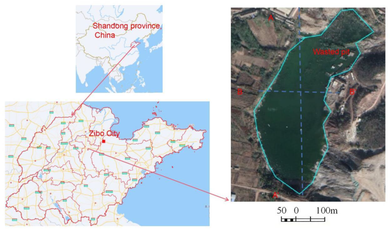
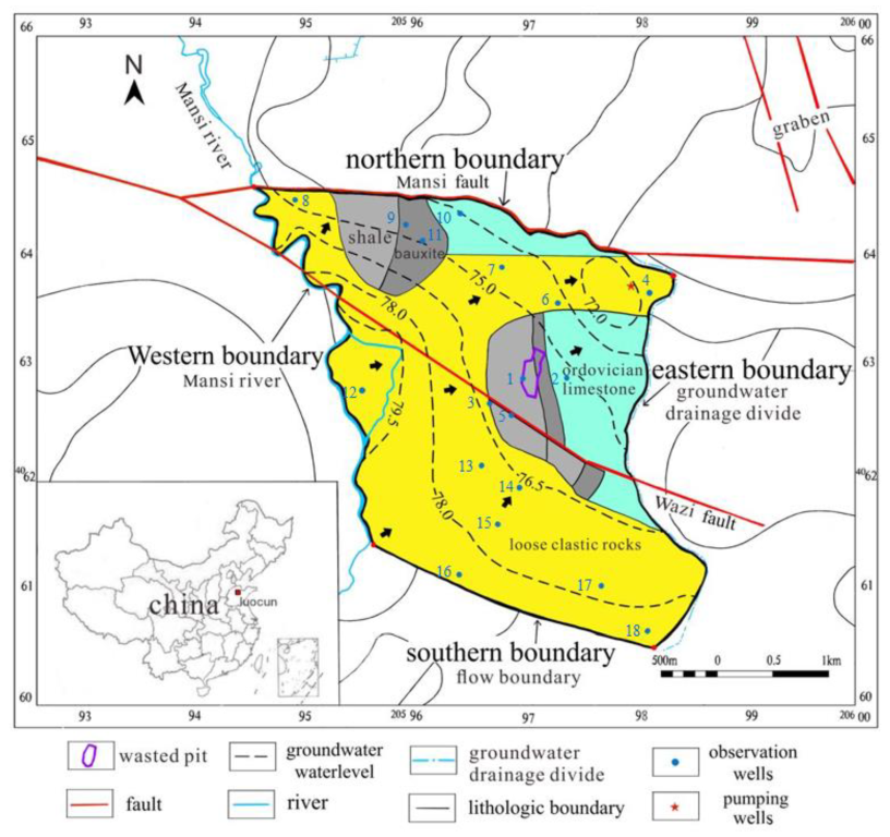
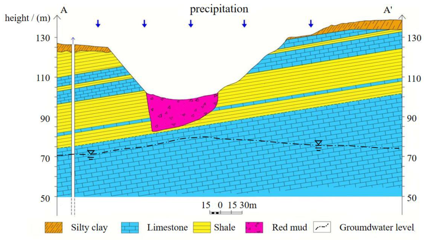
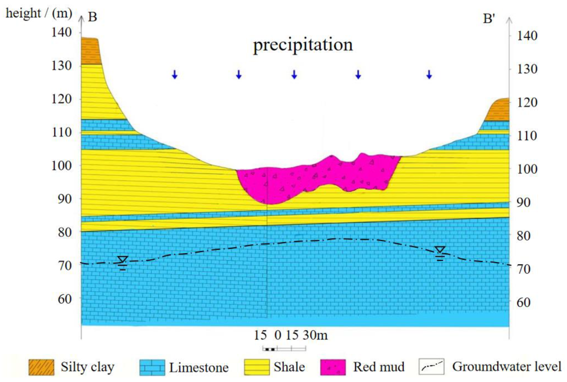
2. Overview of the Study Area

The non-standard red mud tailing pit is situated in northern China (Figure 1). The study area comprises in between 118°02′15′′ N–118°07′09′′ N latitudes and 36°43′11′′ E–36°39′57′′ E longitudes, covering a total area of about 12.692 km2. The average annual precipitation is 671.7 mm, mainly from June to September in the wet season. The average annual evaporation is 1 345.7 mm. The main river in the study area is the Mansi River, located in the west of the study area. Generally, there is surface flow only from September to October in the wet season, and the recharge to groundwater is weak. The main exposed strata (Figure 2) in the study area are Quaternary (Q), Carboniferous-Permian (C-P) and Ordovician (O). Among them, the Ordovician strata are mainly carbonate sedimentary strata, located in the northern part of the study area, trending northeast, dipping southwest, with a dip angle of about 10°. The Ordovician lithology is limestone, dolomitic limestone and dolomite (Figure 3 and Figure 4). With a large variation in production near the fracture zone, its karst fissure are extremely developed, which is the main water recharge source of the main aquifer and local groundwater in the study area. The Carboniferous and Permian strata are distributed in the piedmont of the study area, and strip exposed in the northwest of the Ordovician strata. The bauxite mudstone and shale of Benxi Formation are mainly exposed in the study area. The bauxite mudstone of Benxi Formation is the main source of local bauxite. The red mud tailing pit after bauxite mining by the aluminum refinery is located here. The average thickness of Quaternary stratum is 25 m, mainly composed of gravel, sand and a small amount of clay, which is discontinuous in some areas of the study area.
The study area is located in the plate uplift zone, affected by multi-stage tectonic activities, with many folds and faults in the area, and the terrain is mostly mountainous and hilly. Based on the distribution characteristics of faults in the whole region, the faults basically strike west-east, and the stratum integrity is damaged. Under the action of long-term water flow, the karst phenomenon of karst pipelines or fissures is developed, and groundwater is mainly stored in the corrosion fissure network of faults, joints and bedding fissures [10].
The water recharge of Ordovician limestone aquifer under the red mud tailing pit mainly comes from atmospheric precipitation recharge, river infiltration recharge and lateral recharge of the south flow boundary. The upper phreatic aquifer flows along the terrain and discharges to the northeast. The lower Ordovician limestone aquifer is controlled by regional structure and topography, and the runoff direction is basically consistent with the upper phreatic water.

3. Groundwater Pollution Sources

After the bauxite deposit in the study area was mined, the red mud was directly stacked in the tailing pit (Figure 1), which is in direct contact with the broken Ordovician limestone fissure karst aquifer in the form of a “skylight + water-conducting fissure zone” combination. The red mud leachate generated by rainfall could directly enter the limestone fissure aquifer, which contains alkali, fluoride and other pollutants [11]. According to the satellite image survey, the red mud tailing pit have been leaching the surrounding areas of the pit and groundwater after soaking and leaching for at least 15 years [12].
Water samples were taken from the observation wells of the contaminated site (As shown in Figure 1) and tested with hash DR2800 spectrophotometer. The results are shown in Table 1. Compared with the Groundwater Quality Standard (GB14848-2017) in China for class III quality standard, F, SO42−, Al3+ and other ions exceed the standard, of which F exceeds the standard with the highest frequency (100%). The distribution of F shows obvious gradient distribution characteristics, with many exceeding standard sites, with wide coverage that are harmful to human health. Therefore, this paper took the red mud tailing pit as non-point sources of pollution and selected F as the main characteristic pollutant.

4. Construction of Numerical Simulation Model

4.1. Hydro-Geological Conceptual Model

According to the stratum lithology, thickness and hydro-geological parameters revealed by the drilling data and surface elevation data, the whole stratum can be generalized into two layers vertically, which are the overlying stratum and Ordovician limestone aquifer. According to the drilling data, the top and bottom plate elevations of each layer were obtained by the kriging interpolation method. The conceptual model of groundwater flow was established by using the MODFLOW module in GMS, with a 50 m spacing grid with two layers and three surfaces (Slice) in the vertical direction, for a total of 177,400 effective cells. The simulation period was from 1 January 2003 to 31 December 2019, with three months as a stress cycle. Finally, the aquifer in the study area was generalized as a heterogeneous anisotropic three-dimensional unsteady flow groundwater system.

4.2. Mathematical Model

Through the analysis of hydro-geological conceptual model in the study area, the above heterogeneous anisotropic karst fissure aquifer can be described by the groundwater flow continuity equation and its definite solution conditions [13]. The Formulas (1)–(4) are as follows:
x K xx H x + y K yy H y + z K zz H z + W = μ s H t x , y , z Ω , t 0
Initial   heads : H x , y , z , t t = 0 = H 0 x , y , z x , y , z Ω
Constant   head   boundary : H x , y , z , t Γ 1 = H 1 x , y , z Γ 1 ,   t 0
Zero   flow   boundary :   K n H n Γ 2 = 0 x , y , z Γ 2 , t 0  
where: H is the aquifer head (m); Kxx, Kyy and Kzz are the permeability coefficient in the x, y and z directions (m·d−1); H0 is the initial water level of the flow field (m); H1 is the river water level (m); Kn is the permeability coefficient in the normal direction of the Γ2 boundary (m·d−1); μs is the unit storage coefficient (L−1); W is the source and sink (d−1); Ω is the analog range; Γ1 is the constant head boundary (Dirichlet boundary); Γ2 is the Zero flow boundary or hydraulic barrier boundary (Neumann boundary); n is the outer normal direction of the Γ2 boundary.
The pollutant transport was simulated with the MT3DMS module in GMS. According to the characteristics of the groundwater system, the groundwater solute transport in the study area was analyzed, and the corresponding groundwater solute transport Equation (5) [14] and the initial concentration condition (6) was established as follows:
c t = x ( D xx c X ) + y ( D yy c y ) + z ( D zz c z ) ( u x c ) x ( u y c ) y ( u z c ) z x , y , z ϵ Ω , t 0
c x , y , z , t t = 0 = c 0 c , y , z , t   x , y , z ϵ Ω , t = 0
where: Dxx, Dyy, and Dzz are the dispersion coefficient in x, y and Z directions (m2/d); ux, uy, and uz are the actual flow velocity in three directions (m/d); c is the solute concentration (mg/L); c0 is the initial concentration (mg/L).

4.3. Boundary Conditions

According to the measured flow field and regional hydrogeological conditions, the eastern, southern and northern boundaries of the study area are generalized as constant flow boundaries, including some zero flow separation boundaries. The eastern boundary is the groundwater ridge, which is set as the zero flow boundary; the western boundary is the Mansi River, which is set as the constant head boundary. According to the measured results of the river, it is set as 80 m from south to north; the southern and northern boundaries are set as constant flow boundaries, which are determined to be 2.5 × 10⁴ m3/d according to the hydrogeological survey results. The upper boundary selects atmospheric rainfall as the infiltration boundary and rainfall as the main recharge source. According to the monthly rainfall data provided by the local meteorological bureau and the multi-year average rainfall infiltration coefficient of 0.326, the daily rainfall infiltration is calculated as the surface recharge for the assignment. The Ordovician limestone with a buried depth of 500 m is selected as the bottom boundary of the model.
Generally, the pH value has an important effect on the leaching of fluorine [15]. By collecting fresh red mud samples and soaking them for 30 days, the maximum leaching concentration of F was detected to be 60.0 mg/L after 30 days of leaching at a pH of 10.0 or so. This value is used as the initial maximum concentration of the pollution source in the simulation. Considering that the red mud tailing pit covers 25,342 m2, it is regarded as a surface pollution source in the model simulation. The red mud tailing pit is set as the specified concentration recharge area, and the pollutant concentration in other areas including the boundary is set to zero.

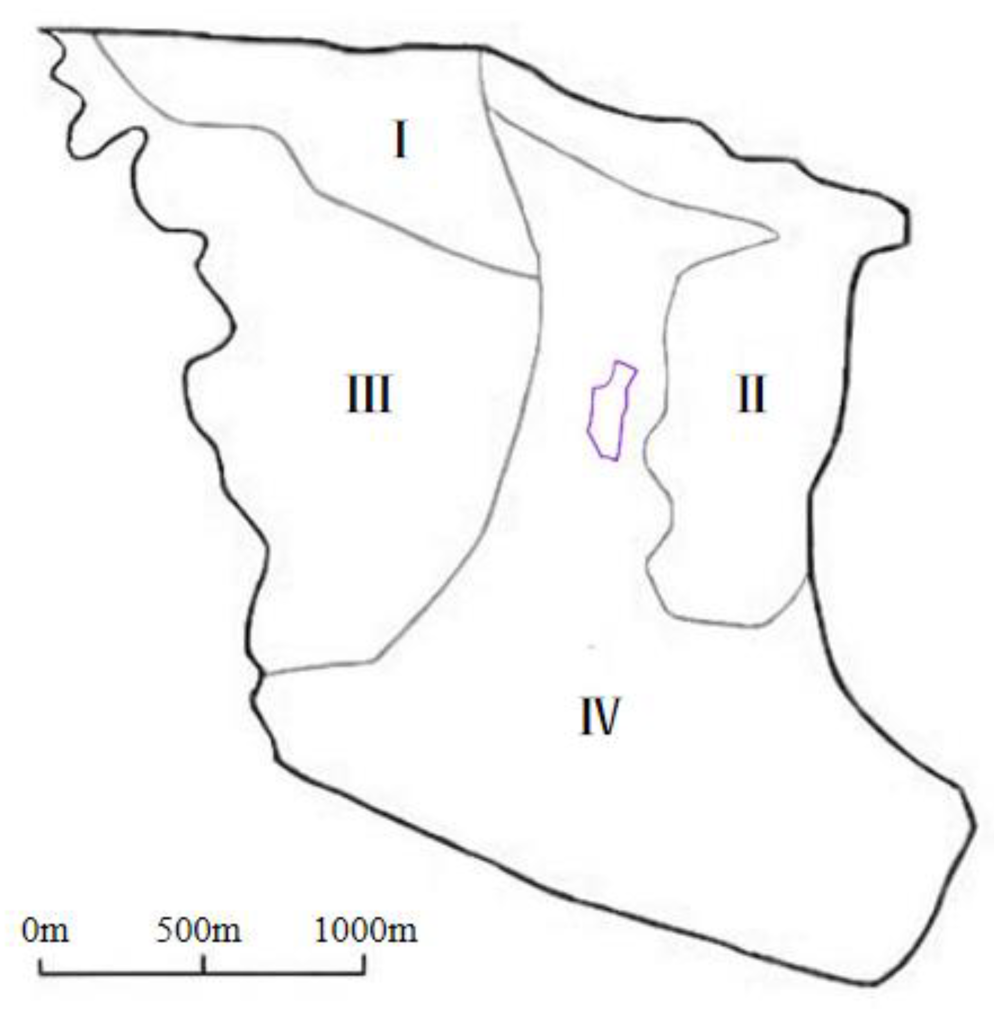
4.4. Parameter Partition and Value

Hydro-geological parameters are very important in groundwater numerical simulation. Their rationality and correctness will directly affect the accuracy and reliability of the groundwater model. Hydro-geological parameters are determined and assigned according to regional pumping test and tracer experiments (Figure 5). The tracer experiment used ammonium molybdate as the tracer and the JP-2 polarograph combined with the standard curve comparison method to determine the concentration of Mo6+. Draw the time and concentration curve according to the detection results of each receiving point, and calculate the permeability coefficient (K) and Longitudinal dispersivity (α) of groundwater aquifer [16]. The calculation formula is as follows:
  α = ( t 1 t 2 ) ( x 2 U 2 t 1 t 2 ) 4 Ut 1 t 2 In ( C 1 t 1 C 2 t 2 )
where: C1, C2 are the concentrations of tracers detected at t1 and t2, respectively (mg/L); x is the distance from the detection hole to the source hole (m); U is the groundwater velocity (m/d).
K = U J  
where: J is the hydraulic gradient (m/m).
The initial values of other parameters are the empirical values of specific yield, storage rate, effective porosity, river infiltration coefficient and other parameters of corresponding lithology [17], and the vertical permeability coefficient was set as 1/10 of the horizontal permeability coefficient. Table 2 were final parameter values.

5. Model Calibration

In this unsteady flow model, the simulated flow field calculated by the MODFLOW module was used as the initial flow field, and the parameter estimation module in GMS software was used to automatically identify and correct the three-dimensional groundwater numerical model to obtain the hydrogeological parameters of the flow model. The root mean square (RMSE) and correlation coefficient (R) were selected as the identification conditions. When the RMSE of the calculated value and the simulated value was the smallest and R approached 1, the most accurate model parameters were obtained.
RMSE = 1 N i = 1 N h i h i obs 2
R = h i h ¯ i h i obs h ¯ i obs h i h ¯ i 2 h i obs h ¯ i obs 2
where: N is the number of groundwater head data (N = 82); hi is the simulated value of the groundwater head; hiobs is the measured value of groundwater head; h ¯ i and h ¯ i obs are the average of the simulated value of groundwater head and the measured value of the groundwater head.

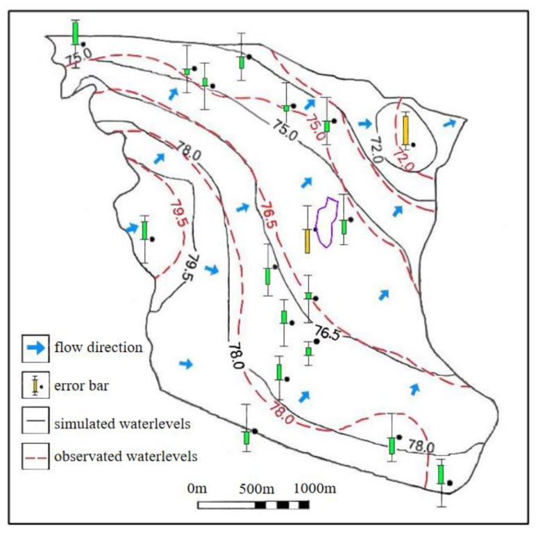
5.1. Groundwater Flow Field Simulation

The observed groundwater table in the study region was observed within 70~80 m, which well corroborate with the Zhu X(2000) results for the same study area. The MODFLOW groundwater simulation results are shown in Figure 6. The color error bars were used to show a MODFLOW calibration, and the center of the target bar signifies the observed head value whereas, the top of the error bar corresponds to the observed value plus the confidence interval and bottom of the error bar represents the observed value minus the confidence interval. If the simulated values lie entirely within the target, the color bar is drawn in green. If the simulated value is outside the target but the error is less than 200%, the bar is drawn in yellow. Whereas if the error greater than 200%, the bar is drawn in red.
The confidence interval of the instantaneous head of observation well was set as 1 m, and the confidence of each observation well was 95%. The groundwater heads of 18 observation wells were recorded in the study area. In Figure 6, the RMSE between the simulated and measured values of all observation wells is 0.95 m; the overall correlation coefficient reaches 0.970. In this study area, 89% of the error bars are green, and only the water level error bars at the discharge outlet in the northeast corner and the red mud tailing pit are yellow. On the whole, it can be considered that the simulation results of the groundwater flow field are consistent with the current groundwater flow field in the study area.

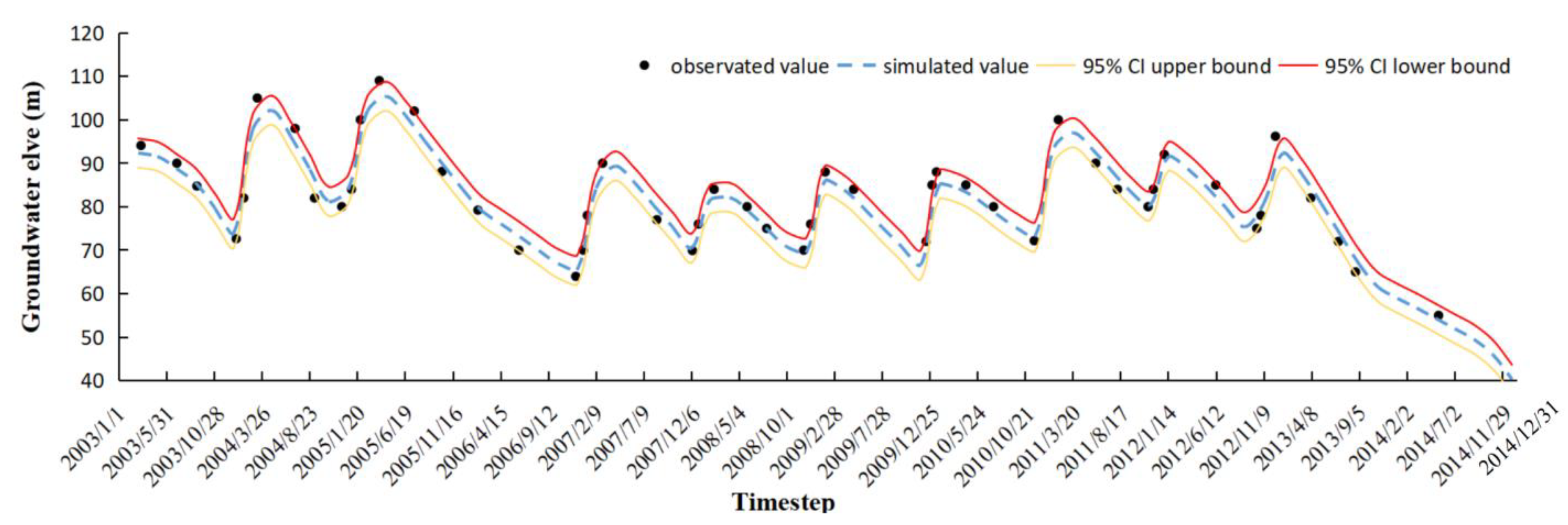
5.2. Multi-Year Water Level Calibration

From the multi-year water level data of the groundwater observation well, the period from January 2003 to December 2014 (144 months) was selected as the simulated stress period, and the groundwater flow model was run to obtain the observation groundwater level fitting results in different periods (Figure 7). It has been noticed between a plot of observation heads vs. computed groundwater heads that at the middle of each stress period (i.e., July–August) the limestone fissure aquifer were replenished by rainfall and surface water bodies. Figure 7 shows that 92% of the water level fall within the confidence interval of the simulated value. According to the Groundwater Resources Management Model Work Requirements (China, GB/T14497-93), nodes with a relative error of less than 10% must account for more than 70% of the water level node; the accuracy of this calculation can meet the requirements, indicating that the model can accurately reflect the multi-year variation characteristics of the groundwater level in the study area.

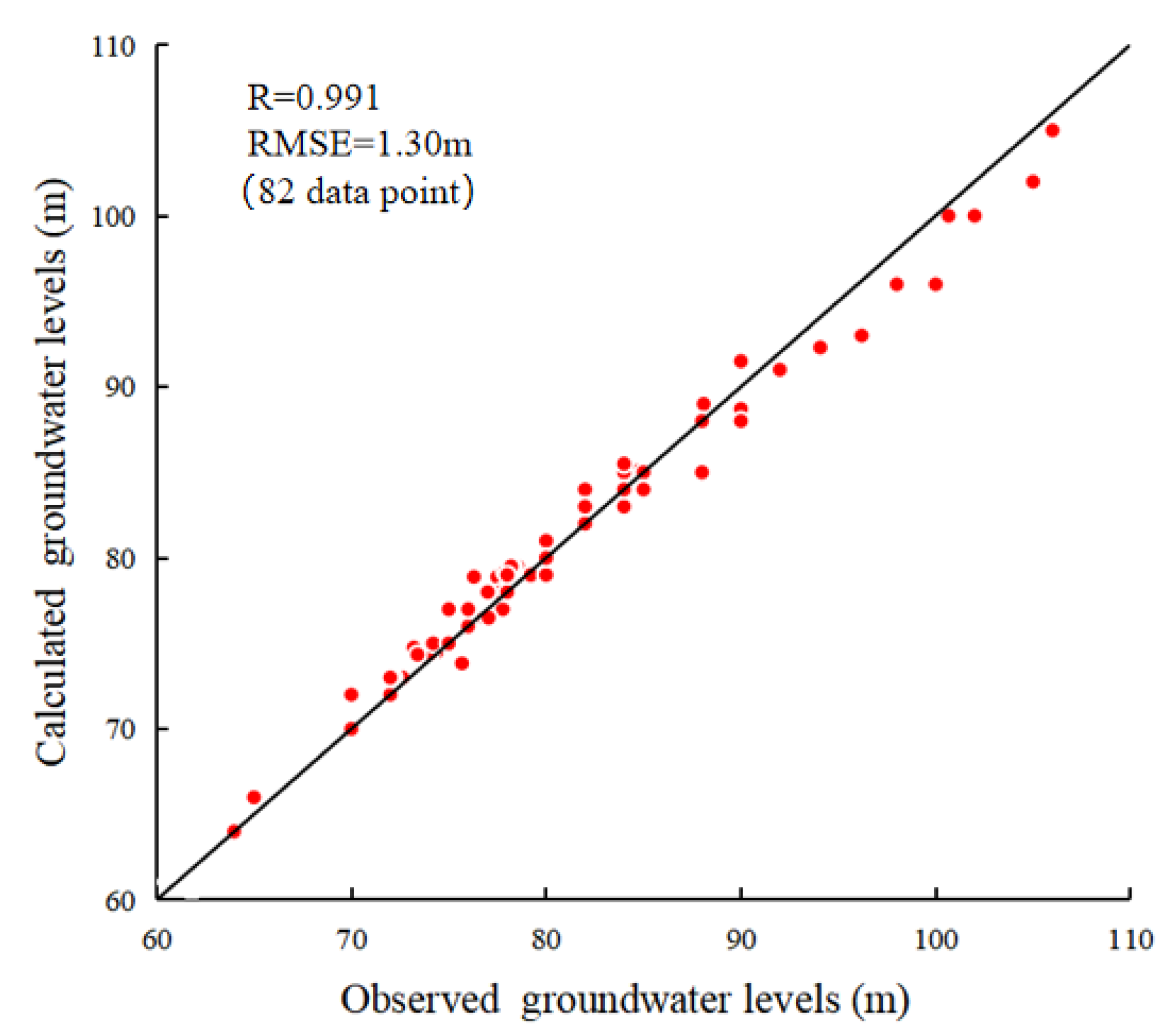
5.3. Observation Water Level Calibration

It can be observed from the simulation results that during the simulation period, the groundwater level demonstrated a downward trend due to the dryness of the local climate and the impact of man-made mining. With the increase in the scope of human activities, the forest coverage area decreases year by year, the soil and water conservation capacity is degraded, and the surface water and the moisture in the unsaturated zone is lost, reducing the recharge of the groundwater.
After running the model, Figure 8 shows the correlation diagram between the simulated value and the measured value. A total of 82 measured values were monitored in all observation wells. In addition, the root mean square error (RMSE) and correlation coefficient were calculated to be 1.30 m and 0.991, respectively, during the simulation time. The fitting result indicated that the simulation model was correct and the parameters were selected reasonably.

5.4. Water Balance Analysis

Further analysis of water balance in the study area: the results (Table 3) show that 65.9% of the groundwater was recharged by the constant flow boundary on the south side, 30.9% was recharged from atmospheric rainfall and 3.1% of groundwater was recharged by rivers. The recharge of the constant head inflow in this area accounts for the least amount of total recharge, indicating that the river’s recharge of groundwater in the region is weak. It is due to the natural surface flow of Mansi River, which has basically been lost because of the pumping project in the study area since the 1950s, with surface flow occurring only during the wet season. A total of 64.2% of the groundwater is discharged from the flow boundary on the north side, 20.7% is discharged from the pumping well, 12.9% of the groundwater is discharged by evaporation and 2.0% of the groundwater is discharged from the river. Combining the recharge volume on the north side and the discharge volume on the south side, it can be found that the constant flow boundary is the main source of groundwater recharge and the main hydrodynamic condition for the formation of the flow field.

6. Simulation Result

This numerical simulation takes into account the maximum initial contaminant concentration and convective dispersion effect of groundwater on pollutants. The research set contaminant concentration observation point at the place was 200 m, 500 m and 1 000 m away from the pollution source along the diffusion direction of the pollutants, respectively (Figure 9), and the concentration duration curve was calculated (Figure 10). The standard value of F is 1 mg/L in accordance with the groundwater quality standard for class III (China, GB14848-2017). When the concentration of F exceeds this value, that means it has exceeded the Chinese national standard.

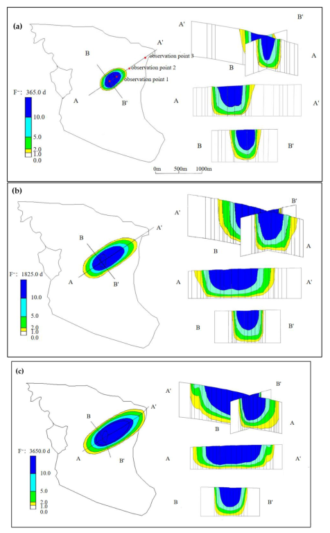
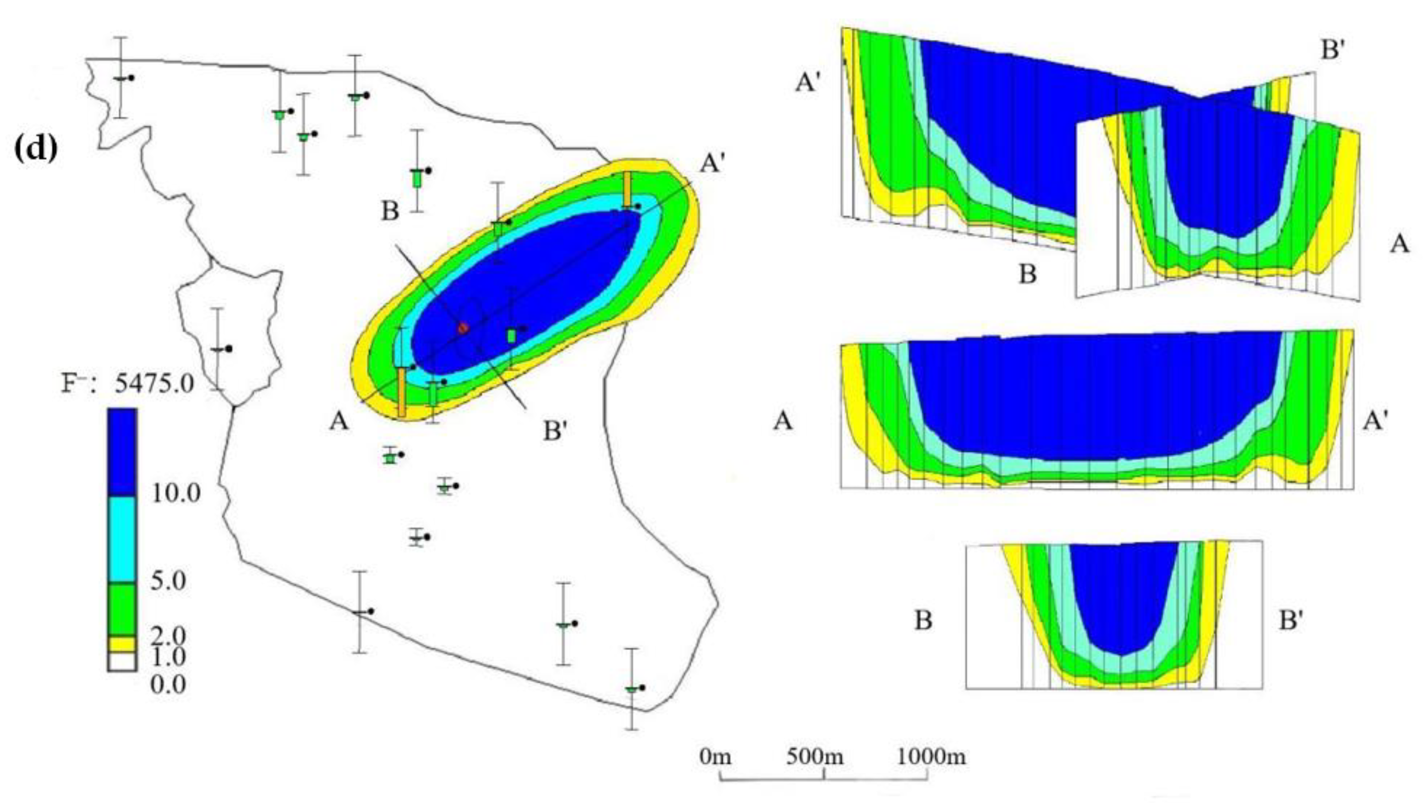
6.1. Distribution of Pollution Plumes

The period from December 2004 to December 2019 (180 months) was selected as the simulated stress period. The simulation results of MT3DMS demonstrate that the pollutant migration was mainly controlled by atmospheric precipitation replenishment, constant flow boundary conditions and leakage of rivers and drainage ditches, which are the main catchment parameters in the study area model at the time of these three factors. The corresponding distribution of pollution plumes at 1, 5, 10 and 15 years after the occurrence of a pollutant spill is shown in Figure 9. As shown in Figure 9d, the results of the transport modeling are successfully validated by F concentration observation data. It can be observed that when the pollution duration was 1, 5, 10 and 15 years, the maximum horizontal migration distances were 473 m, 1160 m, 1595 m and 1750 m, respectively. The pollution center concentration was 60 mg/L, 53.2 mg/L, 45.2 mg/L and 42.3 mg/L, the area of F pollution plumes was 0.37 km2, 1.15 km2, 1.95 km2 and 2.14 km2, respectively. It shows that the vertical pollution of F migration was affected by the hydraulic connection of the aquifer. The maximum vertical influence distance was 492 m, and the pollution of deep aquifers is seriously affected.

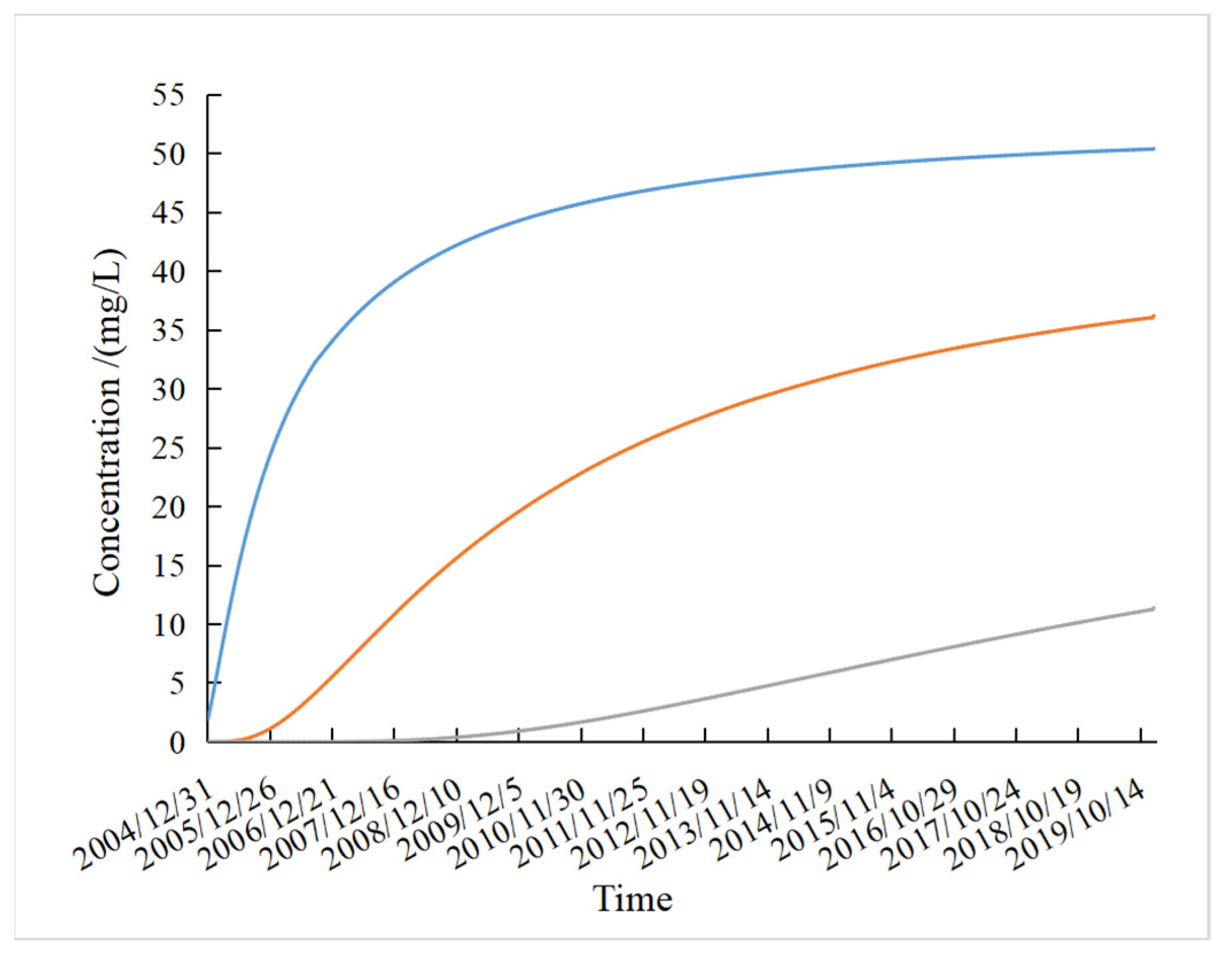
6.2. The Concentration of Pollutants in Different Locations

According to the geological conditions of the red mud pit, after the F pollutant in the red mud pit is leached out from the red mud, it seeps down from the bottom of the pit until it flows to the Ordovician limestone aquifer with a high permeability coefficient.
Figure 10 showed the changes of pollutant concentrations in each observation hole from 31 December 2004 to 31 December 2019. It can be observed from Figure 10 that due to the close distance and continuous leakage at the No. 1 hole, the F concentration increased rapidly and then remained at a high level; no obvious downward trend was observed during the simulation period. In the evaluated period, the maximum concentration of the No. 1 observation well is 50.1 mg/L, No. 2 observation well is 36.2 mg/L, and No. 3 point is 11.4 mg/L, which reflects that the farther away from the pollution source, the lower the pollutant concentration and the concentration gradient, and the smaller the rule.

7. Discussion

7.1. Fitting Error and Parameter Error

Figure 6 shows that the simulated water level of the observation well at the red mud tailing pit is lower than the measured value, which may be due to the complex geological conditions here, where red mud is stacked on the Ordovician limestone aquifer, and the permeability coefficient of the red mud is usually less than 4.5 × 10⁻⁶ m/d [18]. At the red mud tailing pit, the rainwater is difficult to infiltrate, resulting in high simulation value in the pit. The simulated water level of the observation well at the discharge of the groundwater flow field is higher than the measured value, while the Ordovician limestone fissure aquifer in the northeast corner is connected with Mansi fault and directly exposed to the surface to receive atmospheric rainfall recharge, resulting in the simulated value being larger than the actual value.
In Figure 7, there are four observation well data that do not fall within the confidence interval, which are 10 March 2004, 2 April 2005, 1 February 2011 and 15 February 2012, respectively. These four time points are the peak in the annual variation of groundwater level and the four years are all wet years. Through data investigation and analysis, this may be due to the rapid rise of groundwater level caused by heavy rainfall in the wet season of wet years whereas the model rainfall data adopts the average of monthly rainfall data, as the daily rainfall due to the lack of daily rainfall data; thus, an averaging effect occurs, resulting in the low peak value of the simulation value [19].
After model validation and calibrated parameter, the results are shown in Table 2. Table 2 shows that the values of permeability coefficient in different areas of Ordovician limestone aquifer vary greatly. The permeability coefficient of Ordovician limestone aquifer obtained by model inversion is generally large, with a variation range of 1 ~ 20 m/d and a size difference of 20 times, indicating that the karst fissure aquifer has strong heterogeneity.
Generally, the karst is not developed below the depth of 100~150 m of the karst fissure aquifer, and storage coefficient is usually less than 10−4 m−1. However, the storage coefficient of Ordovician limestone aquifer is as high as 9.6 × 10⁻⁴ m−1. According to the rock core and the borehole records, the development depth of karst fissure and dissolved pores in the study area can reach 500~700 m. The total storage capacity of karst fissure aquifer is large and has strong regulation and storage capacity; thus, the water storage coefficient is relatively large [20].

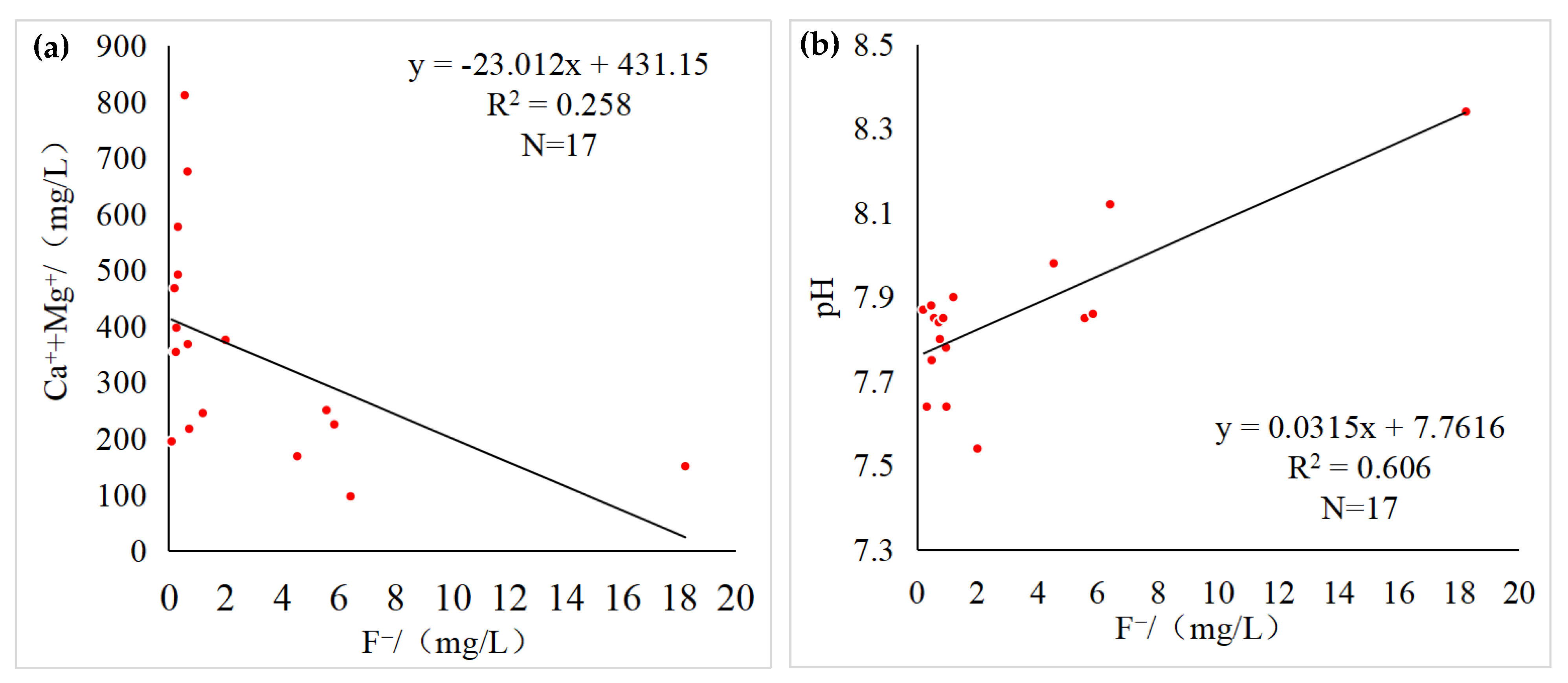
7.2. Precipitation of Fluorine

Water quality monitoring results demonstrated that the maximum migration distance of F was only 1750 m, and the migration distance of pollutants usually reached tens or even tens of kilometers under the long-term convection and diffusion of groundwater, indicating that precipitation occurred in the migration process, and the following reactions could also be existed in the analysis:
Ca 2 + + 2 F CaF 2
Ca 2 + + 2 OH Ca ( OH ) 2
Mg 2 + + 2 F MgF 2
Mg 2 + + 2 OH Mg ( OH ) 2
The relative abundance of main cations in the groundwater of Ordovician limestone is Ca2+ ˃ Mg2+ ˃ Na+ ˃ K+, because there are a lot of limestone (CaCO3), dolomite (CaMg (CO3)2) and fluorite (CaF2) in Ordovician limestone. The high level of Ca2+ and Mg2+ in groundwater is caused by hydrolysis, and the reactions (1) and (3) mainly occur in the initial stage of F entering the groundwater. According to chemical Equation (1) and Equation (3), it can be introduced that at higher initial F concentrations, the increase of Ca2+ and Mg2+ concentration promotes Equations (1) and (3) to move to the right, generating more CaF2 and MgF2 precipitation, and thus reducing the F concentration in the groundwater. Therefore, the concentration of F is negatively correlated with the concentration of groundwater Ca2++Mg2+ (Figure 11a). The leachate of red mud contains a large amount of Al3+, which is prone to hydrolysis reaction and generates positively charged hydrolysate Al2 (OH) 24+, which generates electrostatic adsorption with negatively charged F. Under the combined action of both, the concentration of F in water decreases rapidly. After that, with the migration of pollutants in the groundwater, the content of OH decreased gradually. Under the action of electrostatic adsorption, the F was accelerated to be closer to the adsorption site, resulting in an increase in the adsorption amount of SOIL colloid for F, which resulted in a shorter migration distance of F.
At the same time, previous studies have demonstrated that the acid-base environment of groundwater has a greater impact on F concentration [21], and F concentration is positively correlated with groundwater pH (Figure 11b). The higher the pH value, the excess OH in the solution will combine with the preferentially dissociated Ca2+ to form Ca(OH)2 precipitation, which reduces the concentration of Ca2+, thereby inhibiting the formation of CaF2 in the water, which thus facilitates the enrichment of F in the groundwater. With the flow of groundwater in the aquifer, the pH value of the water gradually decreases, and the abundant Ca2+ in the groundwater will preferentially combine with F to form CaF2 precipitation, resulting in the rapid reduction of F in the groundwater.

8. Conclusions

In this study, the method of combining pumping experiments, tracing experiments and numerical simulations were used to study the fluorine pollution process and diffusion law of red mud pit-polluted Ordovician limestone aquifer groundwater, and the following conclusions were obtained:
(1) A three-dimensional groundwater mathematical model was established for the special red mud pit storage conditions and complex boundary changes in the study area, and the GMS software was used to simulate the migration law of fluorine pollutants in the aquifer. The anti-seepage layer was damaged, and the groundwater pollution plume caused by the red mud yard moved to the northeast as a whole. After 1 year of red mud leachate leakage, the maximum migration distance of pollutant F in groundwater was about 473 m, and the pollution plume range was 0.37 km2. When the leakage occurred for 5 years, the maximum migration distance of F was about 1160 m, and the pollution plume range was 1.15 km2 after 10 years; the maximum migration distance of pollutants in groundwater F was about 1595 m, and the pollution plume range was 1.95 km2. When the seepage occurred 15 years ago, the maximum migration distance of F was about 1750 m, and the pollution plume range was 2.14 km2. The maximum vertical influence distance is 498 m.
(2) The migration of F pollutants in red mud into groundwater was mainly controlled by atmospheric precipitation recharge, flow boundary conditions and seepage in rivers and drains. The simulation results of MT3DMS demonstrated that after 15 years of simulation, the diffusion area of the pollution plume reached 2.14 km2 and then gradually stabilized, indicating that red mud F pollutants have less and less impact on groundwater farther than 1750 m away.
There were some errors in the process of the model simulation, which may be mainly caused by complex hydrogeological conditions and hydrogeochemical reaction factors. The former was mainly due to the influence of structure; the karst aquifer has strong heterogeneity, and there may be strong runoff zones, resulting in high local permeability coefficient and water storage coefficient. Meanwhile the latter, during the migration process of F pollutants, may be associated with complex hydrolysis and precipitation, which leads to some errors in the simulation results.

Author Contributions

Data curation, J.W. (Junping Wang); conceptualization, P.Z. and J.W. (Jiaxin Wu); formal analysis, P.Z.; funding acquisition, Y.Q.; investigation, Y.Q.; methodology, Y.Q.; resources, C.S.; software, J.W. (Junping Wang); writing—original draft, Y.Q.; writing—review and editing, P.Z. and Y.M. All authors have read and agreed to the published version of the manuscript.

Funding

The research was financially supported by the National Natural Science Foundation of China (Nos. 41741020 and 41572218), a project funded by the Priority Academic Program Development of Jiangsu Higher Education Institutions, and the Fundamental Research Funds for the Central Universities (No. 2014QNB51).

Institutional Review Board Statement

Not applicable.

Informed Consent Statement

Not applicable.

Data Availability Statement

Not applicable.

Acknowledgments

This work was financially supported by the National Natural Science Foundation of China (Nos. 41741020 and 41572218), a project funded by the Priority Academic Program Development of Jiangsu Higher Education Institutions, and the Fundamental Research Funds for the Central Universities (No. 2014QNB51). The authors also thank the anonymous reviewers and editors for their constructive comments and suggestions on improving this manuscript.

Conflicts of Interest

The authors declare no conflict of interest.

References

  1. Zhu, Q.S.; Xu, G.Q. The Current Situation and Research Progress of GroundWater Fluorine Pollution in China. Environ. Sci. Manag. 2009, 34, 34–42. [Google Scholar] [CrossRef]
  2. Yi, C.Y.; Wang, B.G.; Jin, M.G. Research Progress of Migration and Transformation Laws of Fluoride in Groundwater-soil-plant System. Saf. Environ. Eng. 2013, 20, 59–64. [Google Scholar] [CrossRef]
  3. Aschonitis, V.G.; Mastrocicco, M.; Colombani, N.; Salemi, E.; Kazakis, N.; Voudouris, K.; Castaldelli, G. Assessment of the Intrinsic Vulnerability of Agricultural Land to Water and Nitrogen Losses via Deterministic Approach and Regression Analysis. Water Air Soil Pollut. 2012, 223, 1605–1614. [Google Scholar] [CrossRef]
  4. He, L.; Tu, C.; He, S.; Long, J.; Sun, Y.; Lin, C. Fluorine enrichment of vegetables and soil around an abandoned aluminium plant and its risk to human health. Environ. Geochem. Health 2021, 43, 1137–1154. [Google Scholar] [CrossRef] [PubMed]
  5. Wang, J.; Zheng, N.; Liu, H.; Cao, X.; Teng, Y.; Zhai, Y. Distribution, Formation and Human Health Risk of Fluorine in Groundwater in Songnen Plain, NE China. Water 2021, 13, 3236. [Google Scholar] [CrossRef]
  6. Yang, J.Y.; Gou, M. The Research status of fluorine cintamination in soils of China. Ecol. Environ. Sci. 2017, 26, 506–513. [Google Scholar] [CrossRef]
  7. Yang, Y.; Li, J.; Li, M.X.; Li, X.; Bai, S.; Xi, B.; Lyn, N.; Yang, Y. Application of HYDRUS-1D model in quantitative assessment of groundwater pollution resource intensity. Chin. J. Environ. Eng. 2014, 8, 5293–5298. [Google Scholar] [CrossRef]
  8. Zhu, X.Y.; Liu, J.L.; Zhu, J.J.; Chen, Y.D. Numerical Study of contaminants transport in fracture-karst water in dawu well field. Chin. Sci. (D) 2000, 30, 479–485. [Google Scholar] [CrossRef]
  9. Sathe, S.S.; Mahanta, C. Groundwater flow and arsenic contamination transport modeling for a multi aquifer terrain: Assessment and mitigation strategies. J. Environ. Manag. 2019, 231, 166–181. [Google Scholar] [CrossRef]
  10. Liu, J.L.; Zhu, X.Y.; Qian, X.X. Study of Some problems on the development and protection of fracture-karst water resources in North China. Acta Geol. Sin. 2000, 74, 344–352. [Google Scholar] [CrossRef]
  11. Hallett, B.M.; Dharmagunawardhane, H.A.; Atal, S.; Valsami-Jones, E.; Ahmed, S.; Burgess, W. Mineralogical sources of groundwater fluoride in Archaen bedrock/regolith aquifers: Mass balances from southern India and north-central Sri Lanka. J. Hydrol. Reg. Stud. 2015, 4, 111–130. [Google Scholar] [CrossRef] [Green Version]
  12. Guo, S.H.; Gao, P.; Wu, B.; Zhang, L.Y. Fluorine emission list of China’s key industries and soil fluorine concentration estimation. Chin. J. Appl. Ecol. 2019, 30, 1–9. [Google Scholar] [CrossRef]
  13. Tong, X.X.; Ning, L.B.; Dong, S.G. GMS Model for Assessment and Prediction of Groundwater Pollution of a Garbage Dumpling Site in Luoyang. Environ. Sci. Technol. 2012, 35, 197–201. [Google Scholar] [CrossRef]
  14. Zhang, Y. Numerical Simulation and Prediction of Contaminated Groundwater in an Animal Protein Production Site by GMS. Geotech. Eng. Tech. 2017, 31, 258–262. [Google Scholar] [CrossRef]
  15. Rong, S.R.; Peng, D.P.; Chen, J.N. Effect of PH Value on Leaching if Rare Mentals from Red Mud in Simulated Natural Storage Conditions. Env. Eng. 2020, 38, 155–159. [Google Scholar] [CrossRef]
  16. Nielsen, D.R.; Van Genuchten, M.T.; Biggar, J.W. Water flow and solute transport processes in the unsaturated zone. Water Resour. Res. 1986, 22, 89S–108S. [Google Scholar] [CrossRef]
  17. Wang, Q.K.; Liang, L.; Chen, C.; Yang, J.Y.; Li, W.; Gong, H.Z.; Zhao, J. Study on Simulations and Control Measures of Leaking Oil Pollution Based on GMS. Environ. Prot. Oil Gas Fields 2018, 28, 12–16. [Google Scholar] [CrossRef]
  18. Wang, G.H.; Zhang, B.J.; Chen, J.H.; Liu, S.C.; Wang, Q.J.; Li, Y.D. Permeation and Migration of Red Mud in Porous Media. J. Water Resour. Archit. Eng. 2020, 18, 1–5. [Google Scholar] [CrossRef]
  19. Yang, Y.; Yin, G.X.; Zhu, L.X. Fluorine Pollution and its Formation Analysis of the Shallow Groundwater in Jiaozuo City. Environ. Sci. Manag. 2009, 34, 68–72. [Google Scholar] [CrossRef]
  20. Li, Q.; Liao, C.N.; Liao, M.X.; Peng, D.P.; Huang, T. Analysis of infiltration mechanism of red mud leachate into sodium-bentonite clay pad. Env. Eng. 2021, 39, 148–153. [Google Scholar] [CrossRef]
  21. Chen, W.; Hao, C.M.; Ma, Z.Y.; Wang, Y.; Zhang, L.; Xu, R.; Chen, P. Geochemical behavior of fluoride in residual coal in groundwater reservoirs. J. North China Inst. Sci. Technol. 2021, 18, 67–73. [Google Scholar] [CrossRef]
Figure 1. Map of wasted pit in the study area.
Water 14 01472 g001
Figure 2. Hydrogeological map of the study area.
Water 14 01472 g002
Figure 3. A-A’ Section.
Water 14 01472 g003
Figure 4. B-B’ section. (the location of the sections was described in Figure 1).
Water 14 01472 g004
Figure 5. Parameter partition diagram of aquifer permeability coefficient.
Water 14 01472 g005
Figure 6. Fitting result of simulated and actual groundwater flow field.
Water 14 01472 g006
Figure 7. Prediction groundwater level at observation well under 95% confidence interval.
Water 14 01472 g007
Figure 8. Scatter plot for observed groundwater level vs. simulated groundwater level.
Water 14 01472 g008
Figure 9. Distribution of pollution plumes in different pollution situations: (a) one year later, (b) five years later, (c) ten years later and (d) fifteen years later.
Water 14 01472 g009aWater 14 01472 g009b
Figure 10. Variation of pollutant concentration in three observation wells.
Water 14 01472 g010
Figure 11. (a) Ca2++Mg2+ and F correlation coefficient diagram; (b) pH and F correlation coefficient diagram.
Water 14 01472 g011
Table 1. Test results of groundwater pollutants.
Scheme 42.F (mg/L)SO42− (mg/L)Al3+ (mg/L)TDS (mg/L)
152.40784.3437.962491.24
218.22663.390.011590.86
36.41205.360.01891.13
45.84216.360.01782.10
55.57275.760.01964.06
64.53408.720.01920.20
72.001529.030.153279.13
81.20378.640.011034.02
Table 2. Initial and calibrated values of hydrogeological parameters in different zones.
ParameterZoneInitial ValueCalibrated
Horizontal permeability coefficient(m/d)I15.017.0
II10.020.0
III0.81.0
IV5.08.0
Porosity (%)I0.10.15
II0.10.25
III0.10.05
IV0.10.10
Specific yield (%)-0.010.02
Specific storage(1/m) 1 × 10−49.6 × 10−4
River conductance (m/d)-3.563.56
Longitudinal dispersivity (m)-5066.7
Table 3. Summary of total MODFLOW simulation groundwater flow budget.
Sources/SinksFlow In
(×104 m3/d)
Flow Out
(×104 m3/d)
Annual Flow In
(×104 m3/a)
Annual Flow Out
(×104 m3/a)
Constant flow boundary2.5432−2.4751964.70866.90
Wells0.0000−0.80000.00292.00
River leakage0.1213−0.081544.2729.75
Recharge1.19250.0000398.760.00
Evapotranspiration0.0000−0.50450.00220.64
Total source/sink3.8570−3.85751407.801408.00
SummaryIn-Out% differenceIn-Out% difference
Sources/sinks−0.00050.0000−0.200.00
Cell-to-cell0.00000.00000.000.00
Total−0.00050.0000−0.200.00
Publisher’s Note: MDPI stays neutral with regard to jurisdictional claims in published maps and institutional affiliations.

