Article

Analysis of the Potential Impact of Climate Change on Climatic Droughts, Snow Dynamics, and the Correlation between Them

by
José-David Hidalgo-Hidalgo
1,
Antonio-Juan Collados-Lara
2,
David Pulido-Velazquez
1,*,
Francisco J. Rueda
2 and
Eulogio Pardo-Igúzquiza
3
1
Instituto Geológico y Minero de España, Departamento de Investigación en Recursos Geológicos, Urbanización Alcázar del Genil, Edificio Zulema Bajo, 18006 Granada, Spain
2
Departamento de Ingeniería Civil, Instituto del Agua, Universidad de Granada, Calle Doctor Severo Ochoa s/n, 18001/Calle Ramón y Cajal, 4, 18003 Granada, Spain
3
Instituto Geológico y Minero de España, Departamento de Investigación en Recursos Geológicos, Ríos Rosas, 23, 28003 Madrid, Spain
*
Author to whom correspondence should be addressed.
Water 2022, 14(7), 1081; https://doi.org/10.3390/w14071081
Submission received: 17 February 2022 / Revised: 11 March 2022 / Accepted: 21 March 2022 / Published: 29 March 2022

Abstract

:
Climate change is expected to increase the occurrence of droughts, with the hydrology in alpine systems being largely determined by snow dynamics. In this paper, we propose a methodology to assess the impact of climate change on both meteorological and hydrological droughts, taking into account the dynamics of the snow cover area (SCA). We also analyze the correlation between these types of droughts. We generated ensembles of local climate scenarios based on regional climate models (RCMs) representative of potential future conditions. We considered several sources of uncertainty: different historical climate databases, simulations obtained with several RCMs, and some statistical downscaling techniques. We then used a stochastic weather generator (SWG) to generate multiple climatic series preserving the characteristics of the ensemble scenario. These were simulated within a cellular automata (CA) model to generate multiple SCA future series. They were used to calculate multiple series of meteorological drought indices, the Standardized Precipitation Index (SPI), Standardized Precipitation Evapotranspiration Index (SPEI), and a novel hydrological drought index (Standardized Snow Cover Index (SSCI)). Linear correlation analysis was applied to both types of drought to analyze how they propagate and the time delay between them. We applied the proposed methodology to the Sierra Nevada (southern Spain), where we estimated a general increase in meteorological and hydrological drought magnitude and duration for the horizon 2071–2100 under the RCP 8.5 emission scenario. The SCA droughts also revealed a significant increase in drought intensity. The meteorological drought propagation to SCA droughts was reflected in an immediate or short time (1 month), obtaining significant correlations in lower accumulation periods of drought indices (3 and 6 months). This allowed us to obtain information about meteorological drought from SCA deficits and vice versa.

1. Introduction

The assessment of hydrological variables requires the application of different models and should consider different sources of uncertainties [1]. Hydrology in alpine systems is largely determined by snow dynamics. In these systems, changes in snow availability can have a significant effect on surrounding ecosystems [2,3], water resources [4,5,6], and tourism [7]. Accumulated snow melt in alpine systems provides an essential water resource to adjacent regions in summer, when precipitation is low [8], thus increasing water availability when demand is high. This exposes the significant ecological and socioeconomic impact associated with low SCA values. A key factor that determines snow dynamics is the weather, which is strongly influenced by elevation [9,10,11]. Climate change models forecast more extreme climate conditions in the future (especially in arid and semi-arid regions) with reductions in precipitation and increases in temperature, which is expected to drastically modify the hydrological regime, affecting both surface and groundwater supplies. Alpine systems in semi-arid regions are highly sensitive to climate change since the hydrological cycle is significantly influenced by snow dynamics (influenced by precipitation and temperature regimes) [12,13,14]. For this reason, the assessment of hydrological droughts associated with snow dynamics is essential to determine the possible impact on water resources.
Drought is a transitory precipitation anomaly that can affect large areas and have devastating effects on agriculture, the environment, and water supplies [15,16]. This negative impact can result in significant economic losses and even social conflict [17] (especially affecting developing countries). Drought is a complex phenomenon that does not have a universal description [18]. A simple definition is to consider it as a water deficit in relation to normal conditions [19]. Depending on the nature of the water deficit, droughts can be categorized into four types: meteorological, hydrological, agricultural, and socioeconomic [20]. Meteorological, hydrological, and agricultural droughts are based on the same concept, i.e., droughts that can be determined as prolonged episodes of unusual arid climate sufficiently extended by water absence, which cause a significant imbalance in the hydrological cycle (low precipitation, soil humidity scarcity, water level decrease, water resource deficits, SCA decrease, etc.) in a region. They are mainly produced by a deficit in precipitation, an increase in air temperature (high evapotranspiration), and a reduction in soil moisture. Despite the fact that drought is a phenomenon that can occur in any region in the world, drought analysis in arid and semi-arid regions is of particularly vital importance, since these are areas with a scarcity of water resources where the adverse effects may be greater due to climate change [21].
In alpine systems, monitoring and analysis of meteorological (precipitation and effective precipitation) and hydrological droughts (associated with SCA) is a key issue given their importance in water resources. Typically, these droughts originate from a meteorological phenomenon that can cause water shortages in other hydrological cycle components (rivers, groundwater, snow, soil moisture, etc.). In recent decades, the scientific community has shown interest in developing drought indices as a tool to monitor and evaluate meteorological drought conditions. The most widely extended indices are defined with multi-scalar properties and are comparable in time and space (SPI, SPEI, etc.). The SPI assesses meteorological droughts in precipitation terms [22] without considering other variables also related to drought occurrence, such as evapotranspiration, wind speed, etc. The SPEI (considered as an enhanced SPI) also takes into account the evapotranspiration effect (in addition to precipitation) to analyze droughts in effective precipitation terms [23]. The mathematical operations proposed to define these indices can be applied to other variables (surface flows, groundwater, SCA, etc.) to evaluate other drought types, such as different hydrological components. An appropriate analysis based on these indices requires the study of series covering long periods [24]. However, in alpine systems, due to difficult access, we usually miss meteorological data with appropriate spatial distribution, especially at higher elevation areas. A feasible alternative is to use climate tools (for example, Spain02, Aemet 5 km, SPREAD and STEAD, etc., databases in Spain) in areas where they are available. These tools offer continuous climate records over a long time period with a fixed spatial resolution. With regard to SCA, this can be obtained from satellite data (e.g., National Oceanic and Atmospheric Administration (NOAA) satellite data or Moderate Resolution Imaging Spectroradiometer (MODIS) satellite data) or models. MODIS provides good accuracy for SCA data [25,26], but in the presence of a dense forest canopy, the uncertainty in the MODIS SCA data increases [27], which reduces the accuracy. A drawback regarding satellite data is that they may be useless during certain periods if cloud cover obscures the view or if there has been a sensor failure. In such cases, alternative tools or models are required to estimate the SCA. So far, SCA has been analyzed using various procedures, including physical-based models, regression techniques, artificial networks, and CA models.
Drought analysis is a topic that has generated interest in the research community in recent years. Numerous studies evaluated the hydrological effect of meteorological droughts on groundwater [28,29,30,31] or surface flows [32,33,34,35,36]. However, to the best of our knowledge, there are no studies that have focused on the relationship between meteorological droughts and hydrological droughts associated with snow dynamics. Neither have we found any studies in the literature that determine the uncertainty of possible climate change impact on meteorological and SCA droughts using multiple climatic series. Regarding spatial scale, most of the studies evaluated drought impact at the basin scale [35,37], as well as regions [38,39,40], countries [41,42,43,44], or entire continents [45,46], but few [47,48] studies focused on alpine systems.
In this article, we propose a methodology to assess the impact of potential future scenarios (downscaled from RCMs) in meteorological and hydrological droughts in alpine systems with two novelties. The first novelty is the analysis of meteorological and SCA hydrological droughts, where we used long, complete series of SCA obtained with a CA model. Different uncertainty sources were considered to generate local scenarios: different historical climate databases, simulations (control scenarios and future scenarios), and different statistical downscaling techniques. We considered the uncertainty in the historical period inherent to different climate products. Secondly, we studied the correlation between meteorological droughts and hydrological droughts associated with SCA. We used the Sierra Nevada mountain range (southern Spain) as a case study, which is a semi-arid alpine system very sensitive to the impact of climate change.
We considered different climate information sources (climate products/databases) to determine the historical drought uncertainty. These climate tools were used to determine meteorological variables (precipitation and effective precipitation), which are necessary to compute the proposed meteorological drought indices (SPI and SPEI). We analyzed the correlation between meteorological drought series and hydrological drought series (SSCI, associated with SCA) to study their relationship within historical and potential future scenarios. We aimed to assess whether information on meteorological drought could be extracted from snow dynamics. Future projections of climate variables (precipitation and temperature) were obtained by downscaling RCMs to adapt them to local conditions. We used equi-probable sets of projections, which provide more robust results than individual models [49,50]. We generated multiple future SCA and climate series (with an SWG) to assess uncertainty in potential future droughts.
This article is organized as follows: Section 2 describes the case study and available data and presents the methodology used to assess the potential impact of climate change and its uncertainty in droughts. Section 3 is dedicated to the analysis of the results. Section 4 discusses the main study aspects. Section 5 presents the main conclusions.

2. Materials and Methods
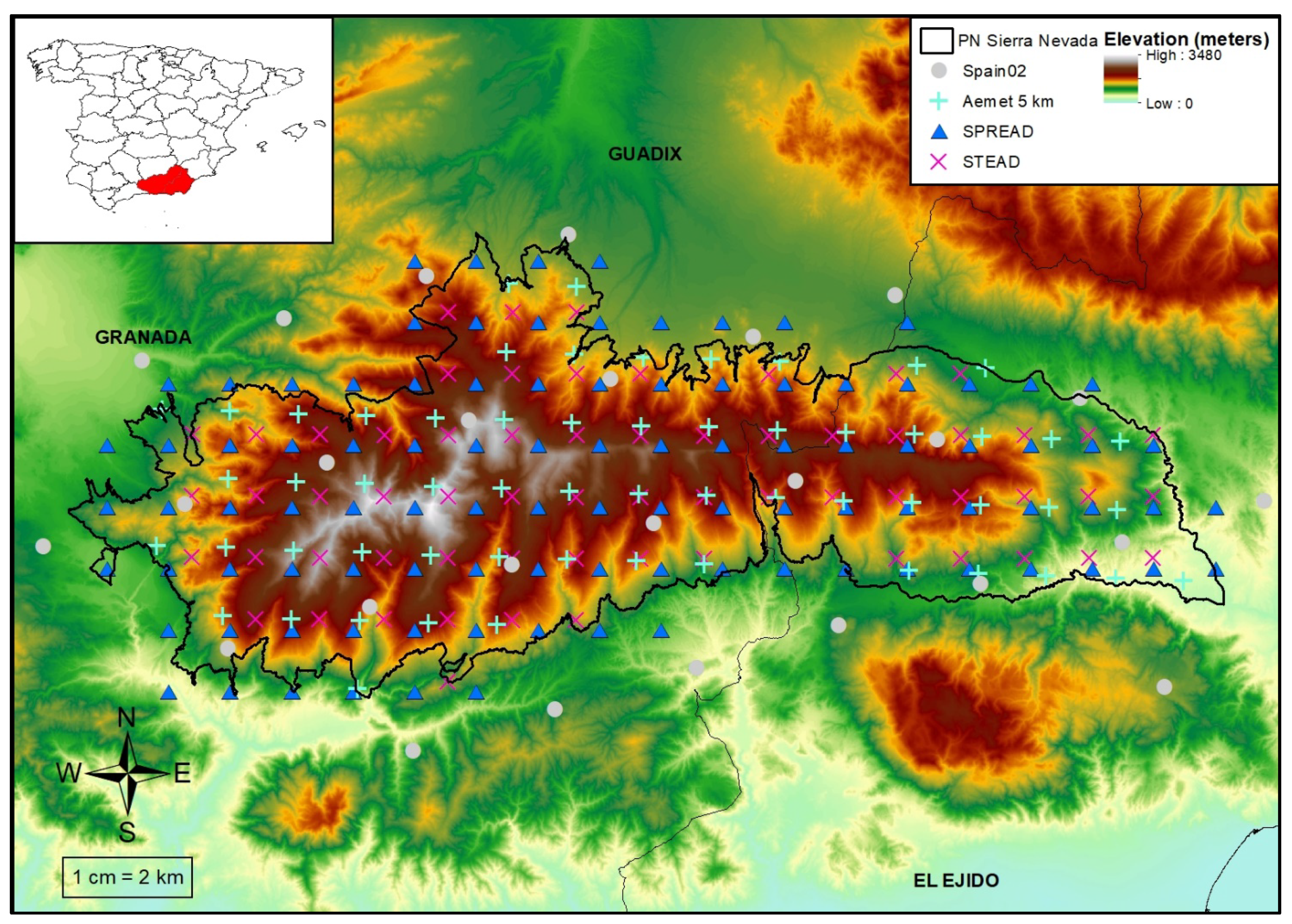
2.1. Study Region

The case study used is the Sierra Nevada mountain range, located in southern Spain (in the provinces of Granada and Almería) (see Figure 1). It is a linear mountain range, 90 km long and 20 km wide, parallel to the Mediterranean coast. It is recognized by several protection agencies (Natural Park, National Park, Biosphere Reserve) and occupies an area of more than 2000 km2. It is one of the highest mountain ranges in Europe, with more than 20 peaks with altitudes above 3000 m This mountain range contains the highest peak in the Iberian Peninsula—Mulhacen—with an altitude of 34,786 m. The Sierra Nevada enjoys a high mountain Mediterranean climate, with dry summers and wetter winters, with precipitation that falls almost exclusively in snow form (from November to May) at altitudes above 2000 m. The snow dynamics have a notable effect on the region from an economic point of view—it is the most southern ski resort in Europe—and from an environmental and water resources perspective, with a hydrographic network that is mainly fed by snow in the melt season. The weather conditions fluctuate temporarily with high spatial variability due to the topography. Due to these particular conditions, it is included in the Global Change in Mountain Regions network [51].

2.2. Datasets and Preprocessing

2.2.1. Historical Weather Data

In this area, various meteorological stations networks are available, which generally have a lack of data at more than 2000 m.a.s.l. In this study, we used different climate tools (Spain02 [52,53], Aemet 5 km [54], SPREAD and STEAD [55,56]) available in Peninsular Spain (given the insufficient climate data spatial distribution at high elevations) to assess the impact of climate change on droughts. We used the historical reference period 1976–2005 as the basis for evaluating climate change signals. The climate data sets used do not provide adequate information on altitudinal gradient due to the low spatial resolution (5 and 12.5 km), so we decided to carry out a drought study referring to the whole of the Sierra Nevada mountain range. We used lumped climate series (using a monthly record weighted average) to homogenize climate records at mountain range scale. The weights were defined as the area represented by each point with information from climate tools by applying the Thiessen polygon method [57].

2.2.2. Spain02

We used historical data provided by the Spain02 project [52,53], which includes daily precipitation and temperature estimates from observations (around 2500 quality-control stations) of the Spanish Meteorological Agency. An assessment of the validation of some Spanish datasets (including Spain02) was recently made by Quintana-Seguí et al. [58]. We used version 5 (v5) of the Spain02 dataset. The project uses the same grid as EURO-CORDEX project with a spatial resolution of 0.11° (approximately 12.5 km). The Spain dataset has already been used in many research studies [59,60]. We only selected climate dataset points included within the Sierra Nevada (or in its vicinity). These points were distributed topographically at heights between 558 and 2420 m (see Figure 1).

2.2.3. Aemet 5 km

The Aemet 5 km project includes daily precipitation and temperature data estimated from 3236 precipitation stations observations and 1800 thermometric stations from the State Meteorological Agency National Data Bank, with a 5 km spatial resolution. We selected 58 stations from precipitation data set (v.2) and temperature data set (v.1) that varied in heights between 647 and 2686 m (see Figure 1).

2.2.4. SPREAD and STEAD

The SPREAD data set [55] contains estimated daily precipitation data from 11,513 observations coming from the State Meteorological Agency, Agriculture and Environment Ministry (MAGRAMA), and regional hydrological and meteorological services stations, with a 5 km spatial resolution. Daily temperature data were obtained from STEAD dataset [56], which includes estimated temperature data from 5056 observations from the State Meteorological Agency and MAGRAMA stations with a 5 km spatial resolution. The climate points selected varied in height from 300 to 3230 m (see Figure 1).

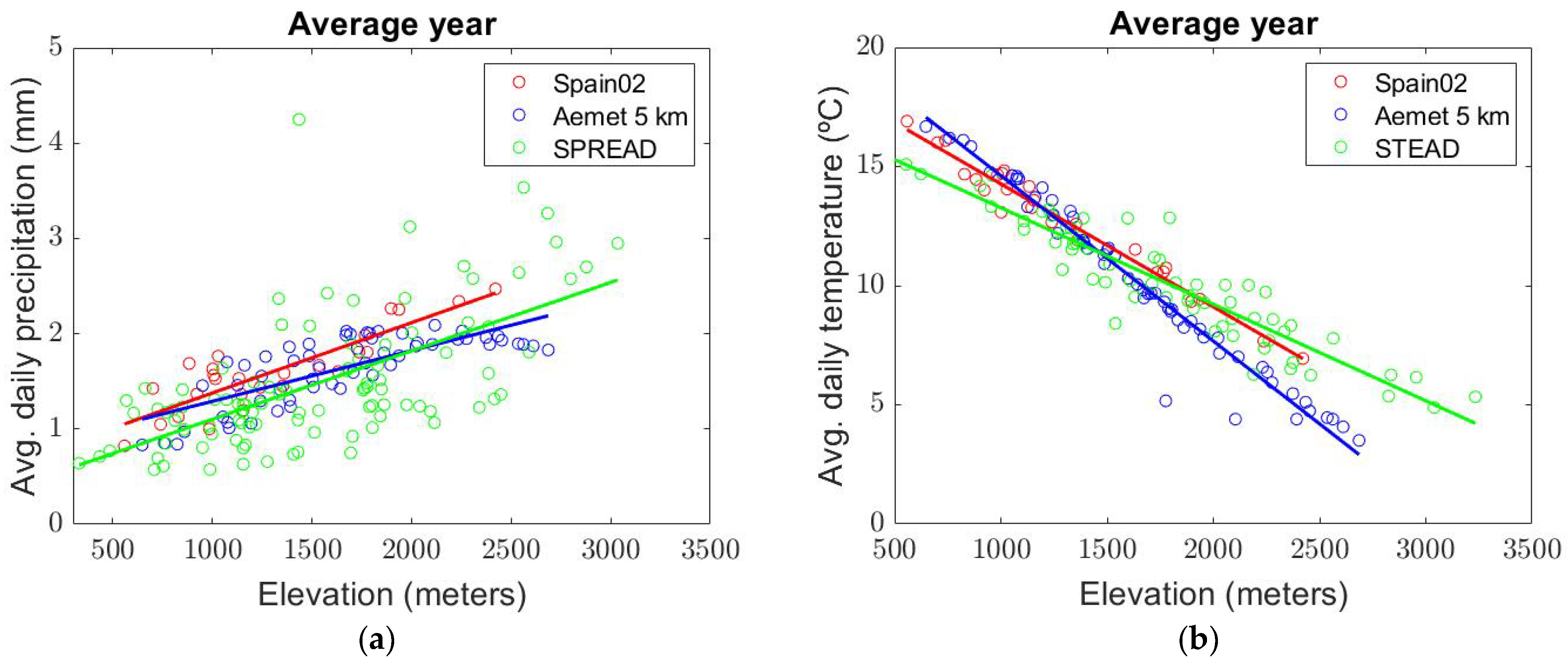
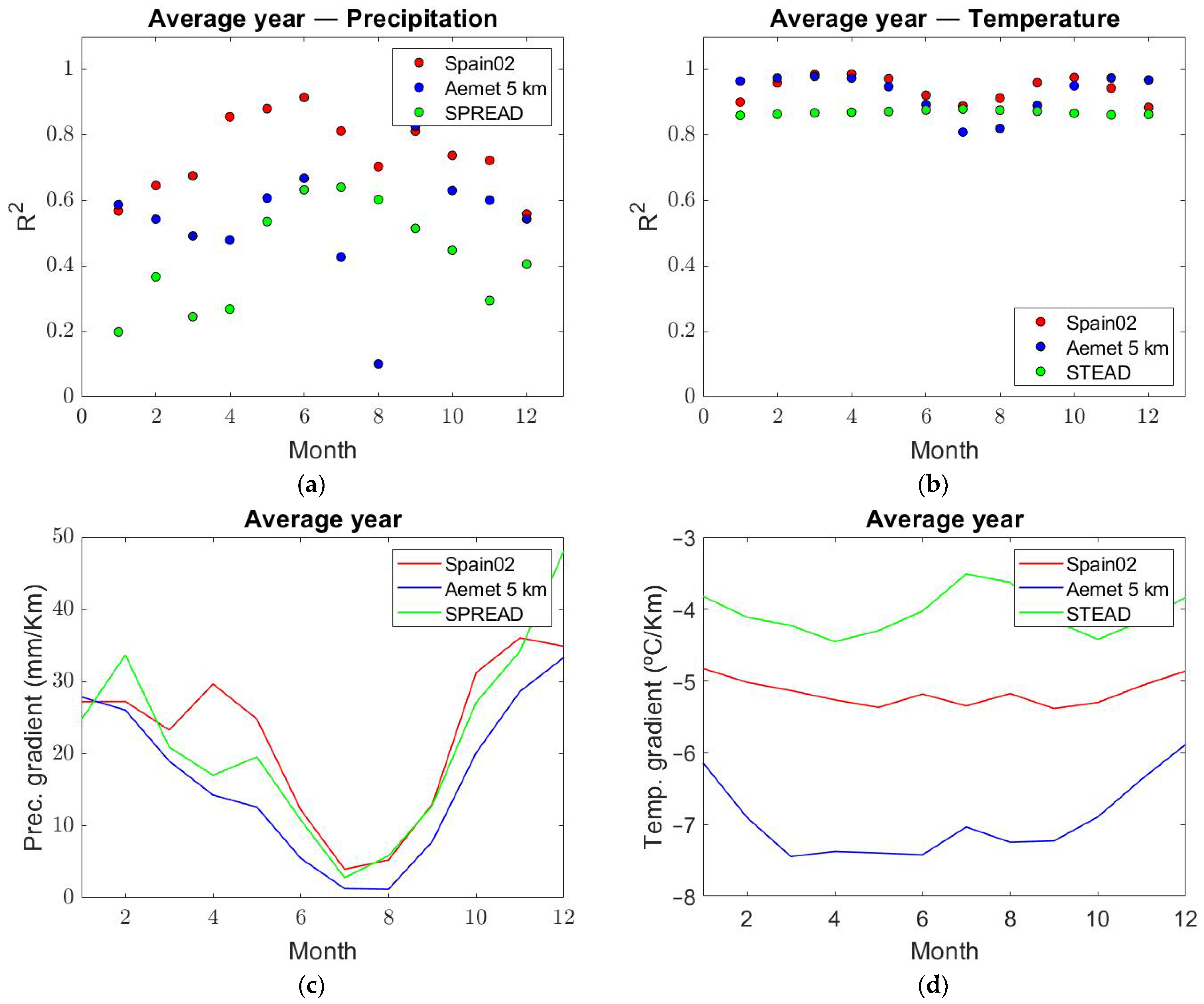
2.2.5. Climate Characterization

Average annual precipitation ranges between 509 and 657 mm year−1 in the Sierra Nevada, mainly occurring between early autumn and spring (October to April). Precipitation is mainly associated with North Atlantic and Mediterranean oscillations [61]. Average annual temperature varies between 9.6 and 11.4 °C, with minimums in January (3 to 5.7 °C) and maximums in August (19.3 to 21.8 °C). These temperatures refer to the whole of the Sierra Nevada National Park, which explains why the minimum temperatures exceed the 0 °C barrier.
We examined the correlation of the climate variables (as an average study time period for the different climate tools) with elevation for the different climate tools. We also analyzed the altitudinal gradient of the climate variables with elevation. Linear correlation with elevation is most evident for temperature, with R2 from 0.87 to 0.97 (see Figure 2b), that for precipitation, with R2 more disparate ranging from 0.4 to 0.76 (see Figure 2a). Precipitation and temperature show marked spatial heterogeneity in the study area (with wide altitudinal gradients), which is common in mountainous regions. Precipitation shows a positive altitudinal gradient (see Figure 2a), with increases in precipitation with altitude. The opposite is observed for temperatures, which decrease the higher the elevation is (showing a negative altitudinal gradient) (see Figure 2b).
Temperature correlations with elevation remain relatively constant throughout the year, with R2 from 0.8 to 0.98 (see Figure 3b). Precipitation shows a more irregular temporal evolution, with R2 from 0.1 to 0.9 (see Figure 3a). The altitudinal temperature gradient with elevation (TAGE) based on mean temperatures shows a clear difference between climate databases. The Aemet 5 km tool shows a pronounced TAGE based on daily means, with lower gradients in winter (−5.9 °C km−1 in December) and more pronounced in spring and summer (−7.4 °C km−1 in March, April, May, and June). In contrast, the Spain02 and STEAD tools show lower TAGE with little variation throughout the year, with gradients that vary between −4.9 °C km−1 in December and −5.4 °C km−1 in May and between −3.8 °C km−1 in December and −4.5 °C km−1 in April, respectively (see Figure 3d). Vertical precipitation gradients are the consequence of air rising and stinking as it passes over the mountain ridge. Its values are positive on the windward side, whilst on the leeward side, the values are negative, increasing when the distance from the mountain increases. In the study area, the altitudinal precipitation gradient with elevation (PAGE) follows the same pattern with different climate tools, with pronounced variations in winter and almost non-existent in summer (see Figure 3c). PAGE based on monthly average precipitation reaches minimum values in summer, with values that vary between +1.2 and +0.058 mm km−1 in August, increasing significantly for the rest of the year (autumn, winter, and spring), with maximum values varying from +33.4 to +48.1 mm km−1 in December (see Figure 3c).

2.2.6. Snow Cover Data

SCA data from the historical period (1976–2005) and future period (2071–2100) were provided from a previous study published by Collados-Lara et al. [62]. In this study, we used a CA model based on one developed by Pardo- Igúzquiza et al. [63] to simulate SCA using climate indices (precipitation and temperature) as descriptive variables and a series of parameters (threshold precipitation, threshold temperature, and threshold in the number of neighbor cells that produce a change in the cell state). This model uses a series of transition rules that allows us to determine the absence or presence of snow. It has been proven to be a useful tool for accurately simulating SCA dynamics [62,63].

2.2.7. Regional Climate Models

We considered the most pessimistic CORDEX project emission scenario (RCP 8.5) [64]. For this scenario, we analyzed nine RCMs nested to four different Global Climate Models (GCMs) (CNRM-CM5, EC-EARTH, MPI-ESM-LR, and IPSL-CM5A-MR). These series (control scenarios and future simulations of the CORDEX EU project) from five RCMs (CCLM4-8-17, RCA4, HIRHAM5, RACMO22E, and WRF331F) nested in each GCM considered were used to assess possible future climate scenarios in the period 2071–2100. RCM simulations considered are summarized in Table 1.

2.3. Methods

We propose a methodology to study historical meteorological and hydrological SCA droughts and the potential future impact on them in alpine regions for different time-aggregation periods (see Figure 4). Several uncertainty sources were considered. The historical information used was derived from different climate products. Local potential future scenarios (based on the historical information) were defined for a specific time horizon (2071–2100) and emission scenario (RCP 8.5) by using different RCM simulations, downscaling techniques, and SWG to generate multiple synthetic series, etc. We analyzed the temporal correlation of SPI/SPEI series (defined to study meteorological droughts) and SSCI series related to SCA dynamics for the study of hydrological droughts. We aimed to draw conclusions about meteorological droughts, which can be inferred from the SCA dynamics series and vice versa. The proposed methodology (see Figure 4) includes the following steps. (1) historical assessment of meteorological (based on precipitation and effective precipitation series) and hydrological SCA droughts and uncertainties (due to the climate product) analysis. (2) Future analysis of meteorological and hydrological SCA droughts: (2.1) define future local scenarios by applying different statistical correction techniques under two conceptual downscaling approaches from RCM simulations included in EURO-CORDEX project; (2.2) multiple climate and SCA series generation by using an SWG that preserves the main statistics of local future scenarios; (3) correlation analysis between meteorological and hydrological SCA droughts for different time lags.
We used two different indices to analyze meteorological droughts: SPI and SPEI. The SCA drought was evaluated with SSCI (applying the same methodology as SPI using SCA data as input). We applied the run theory [65] to determine the drought statistics. It is important to note that the future drought index values were calculated using the probability distributions parameters calibrated for the historical observations for an adequate comparison between the historical and future periods to identify and assess the impact of climate change [66].

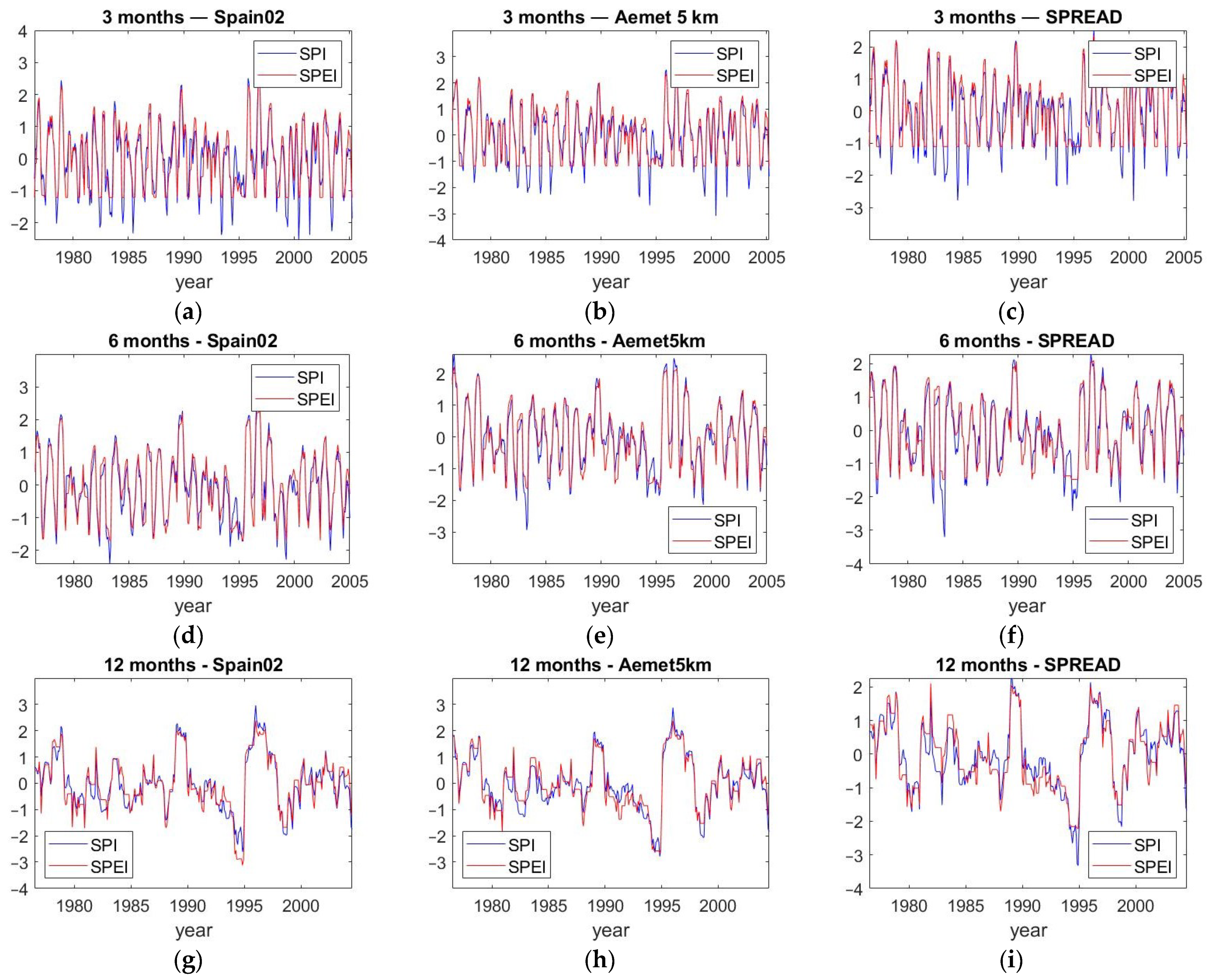
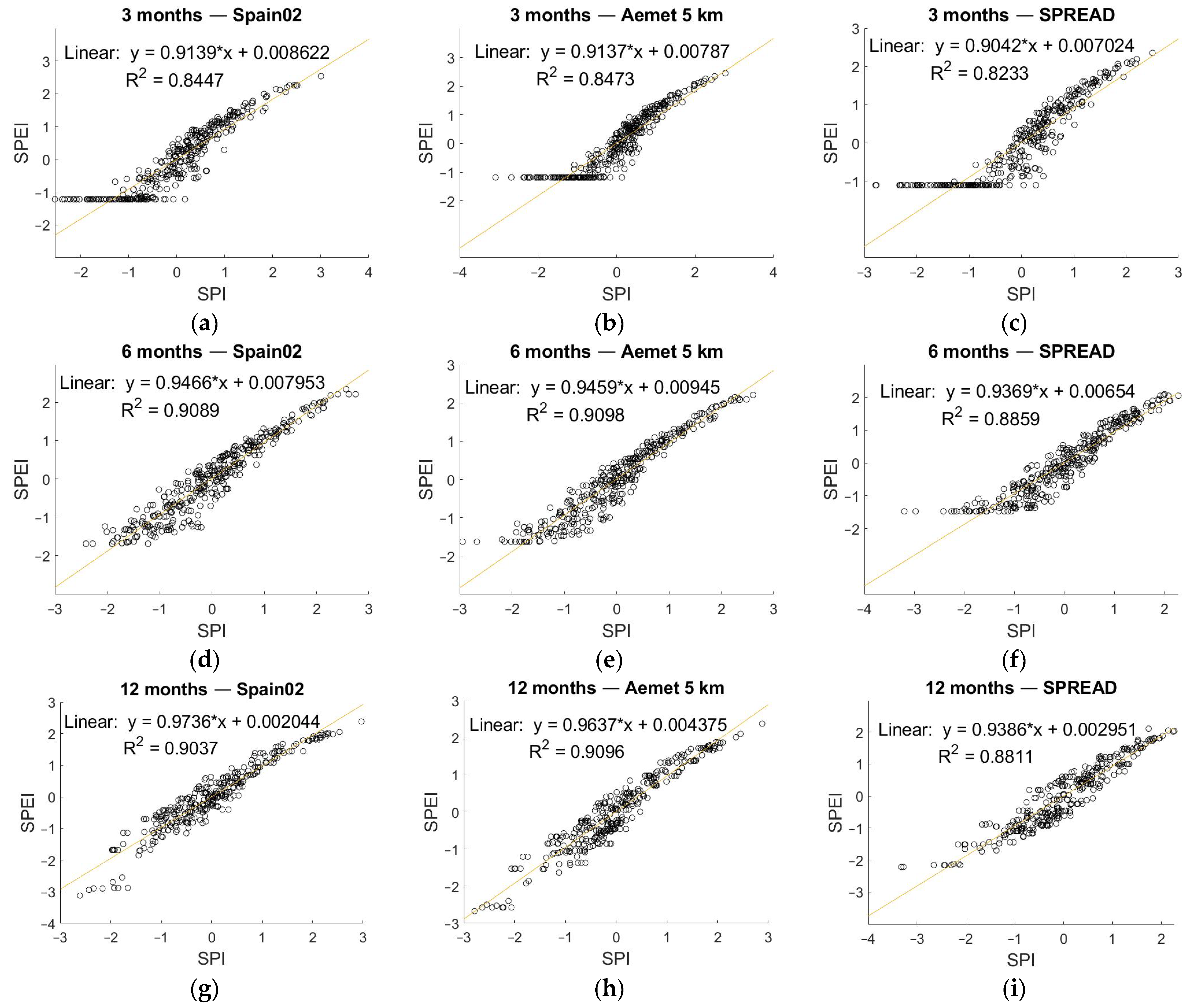
2.3.1. Drought Indices

Standardized Precipitation Index

SPI requires monthly precipitation data as input. It does not take into account other variables also related to drought occurrences, such as temperature, evapotranspiration, wind speed, or atmospheric humidity. This index was developed by McKee et al. [22] for drought analysis and monitoring. The main advantage of SPI is that it can be calculated on multiple time scales, being comparable in time and space [67,68]. In our case study, we calculated SPI for different temporal-aggregation time scales (3, 6, and 12 months). We fitted accumulated precipitation data to a gamma distribution [69] and transformed cumulative probability to a standard normal distribution function, with a mean zero and standard deviation one, which provides SPI values. We used the Abramowitz and Stegun approximation [70] to transform cumulative probability in the SPI value:
SPI = ( t c 0 + c 1 t + c 2 t 2 1 + d 1 + d 2 t 2 + d 3 t 3 )     for   0   <   H ( x )     0.5
SPI = + ( t c 0 + c 1 t + c 2 t 2 1 + d 1 + d 2 t 2 + d 3 t 3 )   for   0.5   <   H ( x )   <   1
where:
t = ln ( 1 ( H ( x ) ) 2 )     for   0   <   H ( x )     0.5
t = ln ( 1 ( 1 H ( x ) ) 2 )     for   0.5   <   H ( x )   <   1
where H(x) is cumulative probability, and the constants are: c0 = 2.515517, c1 = 0.802853, c2 = 0.010328, d1 = 1.432788, d2 = 0.189269, d3 = 0.001308. Positive SPI values indicate wet periods, with deviations above the mean. Negative SPI values indicate dry periods, with deviations below the mean.

Standardized Evapotranspiration Precipitation Index

SPEI developed by Vicente-Serrano et al. [23] (considered an improved SPI) is particularly useful for analyzing climate change effects in drought conditions. The SPEI considers the influence of temperature on drought, preserving the SPI’s multi-scale nature. This index is based on a climate water balance determined by the difference between precipitation and potential evapotranspiration in each month i:
D i = P i PET i
where D is effective precipitation, P is precipitation, and PET is evapotranspiration. Evapotranspiration is calculated by applying the Thornthwaite approximation [71], which only requires the monthly mean temperature values as input.
The SPEI is calculated following the procedure described in Vicente-Serrano et al. [23], where cumulative D series fit a three-parameter Log-Logistic distribution. Di values calculated are added for different time scales (3, 6, and 12 months). To transform the cumulative probability values to the SPEI values, a standard normal distribution, with a mean zero and standard deviation one, is used following the Abramowitz and Stegun approximation [70]:
SPEI = W c 0 + c 1 W + c 2 W 2 1 + d 1 W + d 2 W 2 + d 3 W 3
where W = 2 ln ( p ) to p  0.5, where p is the probability of exceeding a certain value D, p = 1 F ( x ) , where F ( x ) is the cumulative probability. If p > 0.5, p is replaced by 1 p , and the SPEI resulting sign is reversed. The constants are c0 = 2.515517, c1 = 0.802853, c2 = 0.010328, d1 = 1.432788, d2 = 0.189269, and d3 = 0.001308.

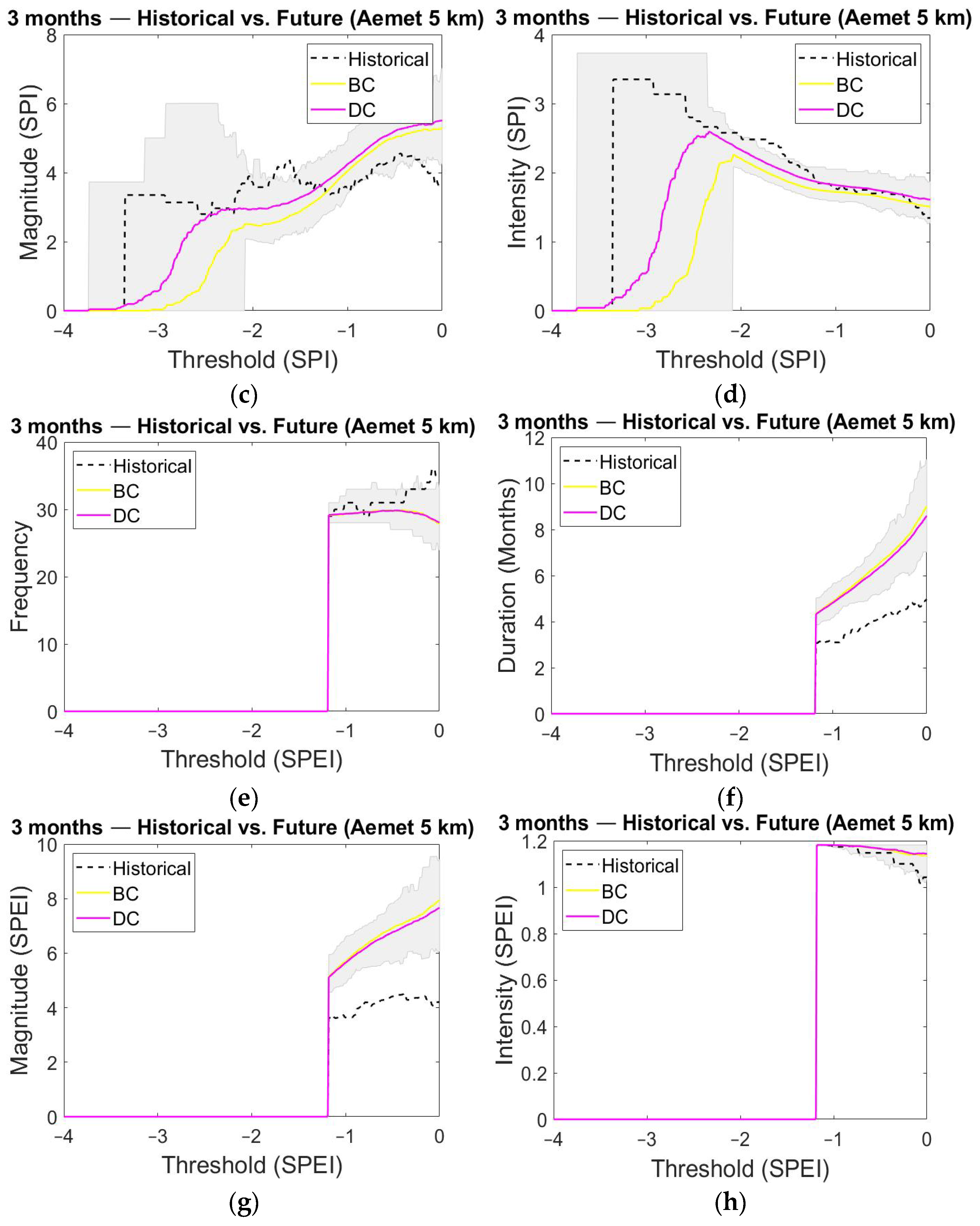
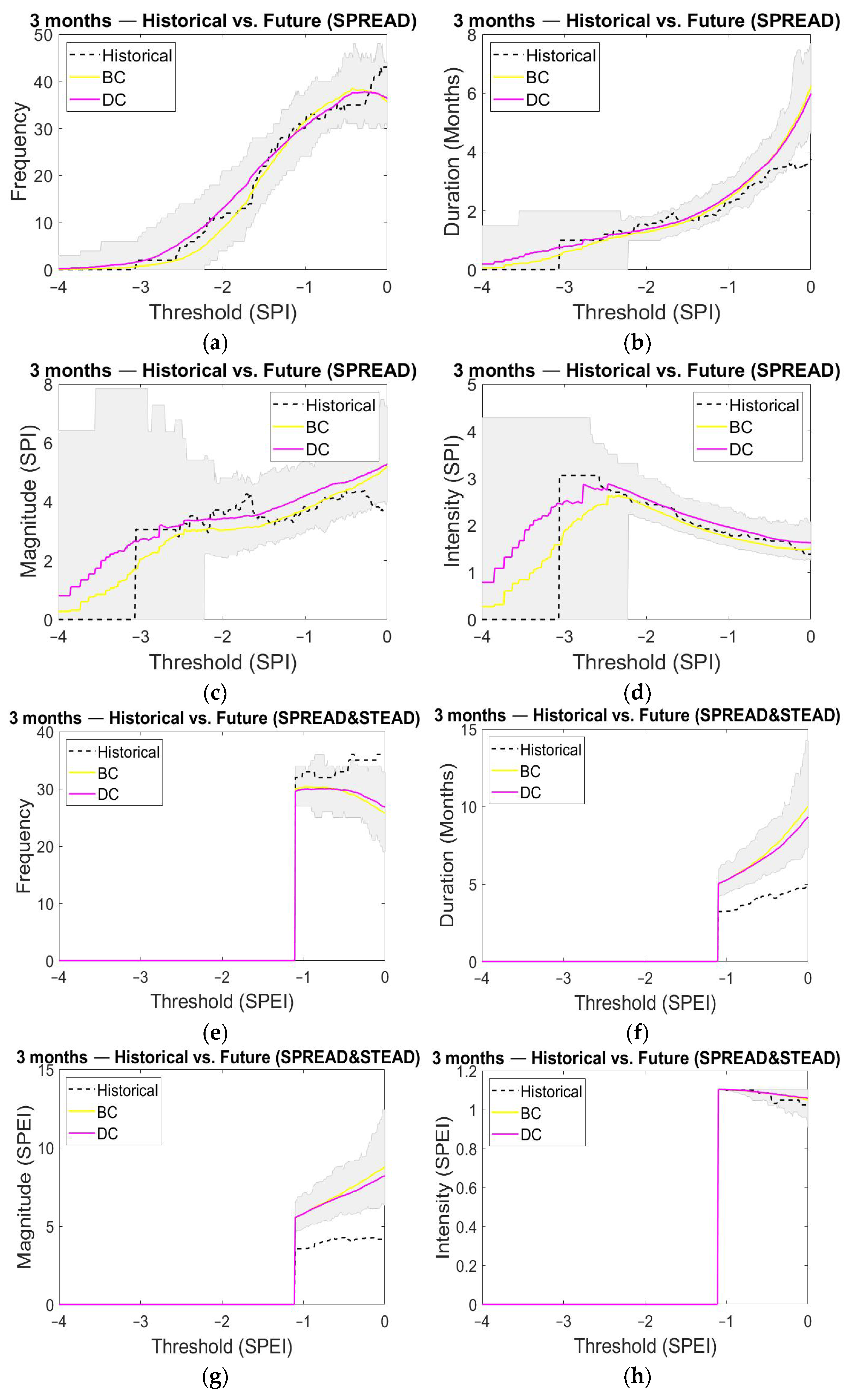
2.3.2. Drought Statistics

Drought statistics (frequency, duration, magnitude, and intensity) were calculated by applying the run theory [65]. We considered meteorological (SPI and SPEI) and hydrological (SSCI) drought index threshold values (ranging from −4 to 0) to identify drought periods. The frequency is defined as the number of drought events during a certain time period. The duration is defined as an uninterrupted time period (in months) with index values below the threshold value. The magnitude is the sum of all the index values during the duration of the drought. The intensity is the minimum index value in a specific drought event. Drought statistics values determined for each drought event were averaged for the total drought events number identified for each threshold.
M = i = 1 D Í NDICE i
I = Min ( Í NDICE D )
where D is the duration, M is the mean magnitude, and I is the mean intensity of the drought.

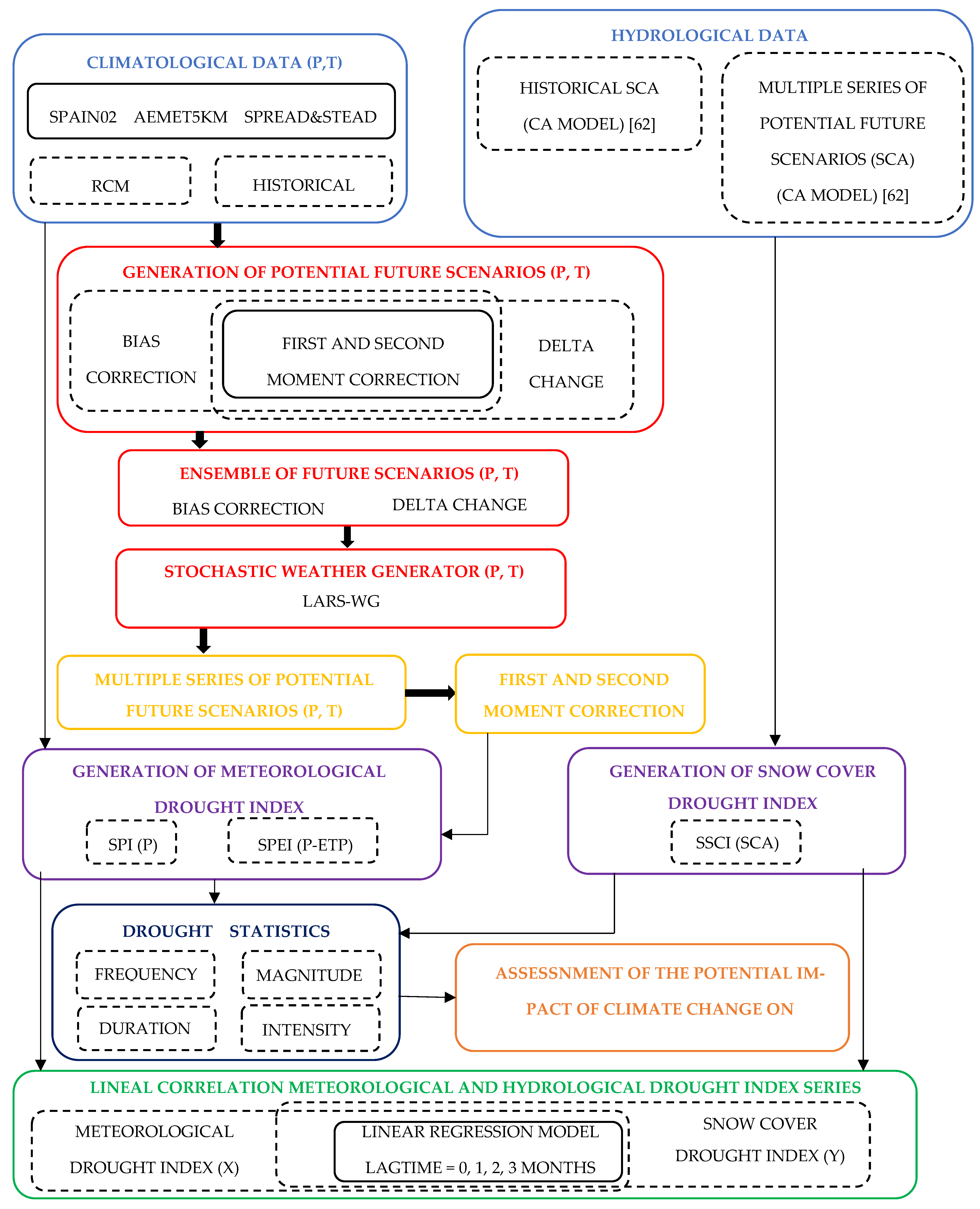
2.3.3. Future Drought Strategy

We proposed an RCM correction to generate local future scenarios that would provide reliable estimates of the climate characteristics (precipitation and temperature). The obtained future climate scenarios were introduced into an SWG to generate multiple climate series to approach future scenarios’ uncertainty. We used this multiple climate series to generate relative drought indices (rSPI, rSPEI, and rSSCI), which were calculated using the probability distributions parameters of the historical series, which allowed us to make an adequate comparison to assess the potential impact of climate change. The generation of multiple drought index series (using an SWG) allowed us to assess climate change uncertainty in droughts. The multiple local future climate scenarios generation procedure is described next and the multiple local future SCA scenarios were obtained from a previous study [72].

Local Future Scenarios

We used a tool developed by Collados-Lara et al. [73,74] for the generation of future climate scenarios considering two different downscaling approaches: bias correction (BC) and delta change (DC). The BC approach applies a transformation function to the control RCM simulation to obtain another with similar statistics to the historical one. The transformation function is applied to the future simulation to obtain a corrected future scenario. It is assumed that bias between the historical series statistics and the control simulation will remain invariant in the future. The DC approach assumes that RCMs provide an accurate assessment of the relative changes between the control simulation and the future simulation and applies these changes to the historical series to obtain a corrected future series. The transformation function applied in both approaches is defined with the first- and second-moment statistical-correction technique. Individual future scenarios generated with the different RCMs were merged, making equi-probable ensembles of future projections with BC and DC approaches, which provide more representative future scenarios.

Generation of Multiple Climate Series Using a Stochastic Model

SWG allows us to generate synthetic time series with statistical characteristics similar to future projection scenarios. These generated multiple future scenarios are consistent with future scenarios predicted with RCMs. The future scenarios generated with BC and DC approaches are used as input in LARS-WG-SWG [75] to generate multiple future series. LARS-WG has been updated several times (most recently in April 2021) and can be used to generate synthetic weather series at a location. It can also be used to generate potential local future scenarios based on Global Climate Models (GCM) outputs. In this study, we used LARS-WG to produce multiple synthetic climate time series based on sets of future local climate scenarios generated with BC and DC approaches (derived from different local RCM projections). Multiple series generated with SWG may show bias with original series statistics. We corrected these biases using a statistical technique developed by Collados-Lara et al. [72] based on mean and standard deviation correction.

Analysis of the Temporal Correlation between Meteorological Drought and Snow Cover Dynamics

We evaluated the correlation degree between meteorological drought and SCA drought by applying a linear regression model. Meteorological drought series were assumed as the independent variable (x) and SCA drought series as the dependent variable (y). Thus, if we consider xi and yi with i = 1, 2, …, N; the linear relationship between variables is determined with the determination coefficient:
R 2 = 1 i = 1 N ( y i y i ^   ) 2 i = 1 N ( y i y ¯ ) 2   with   lag   time = 0 , + 1 , + 2 , + 3   months .
where y ^ =   β 1 x + β 0 is the fitted linear regression line, where β1 and β0 are slope and intercept, respectively, with R2 in the range of (0 ≤ R2 ≤ 1). Determination coefficient specifies the proportion of the independent variable (y) variance that can be linearly attributed to dependent variable (x) variance [76].

3. Results

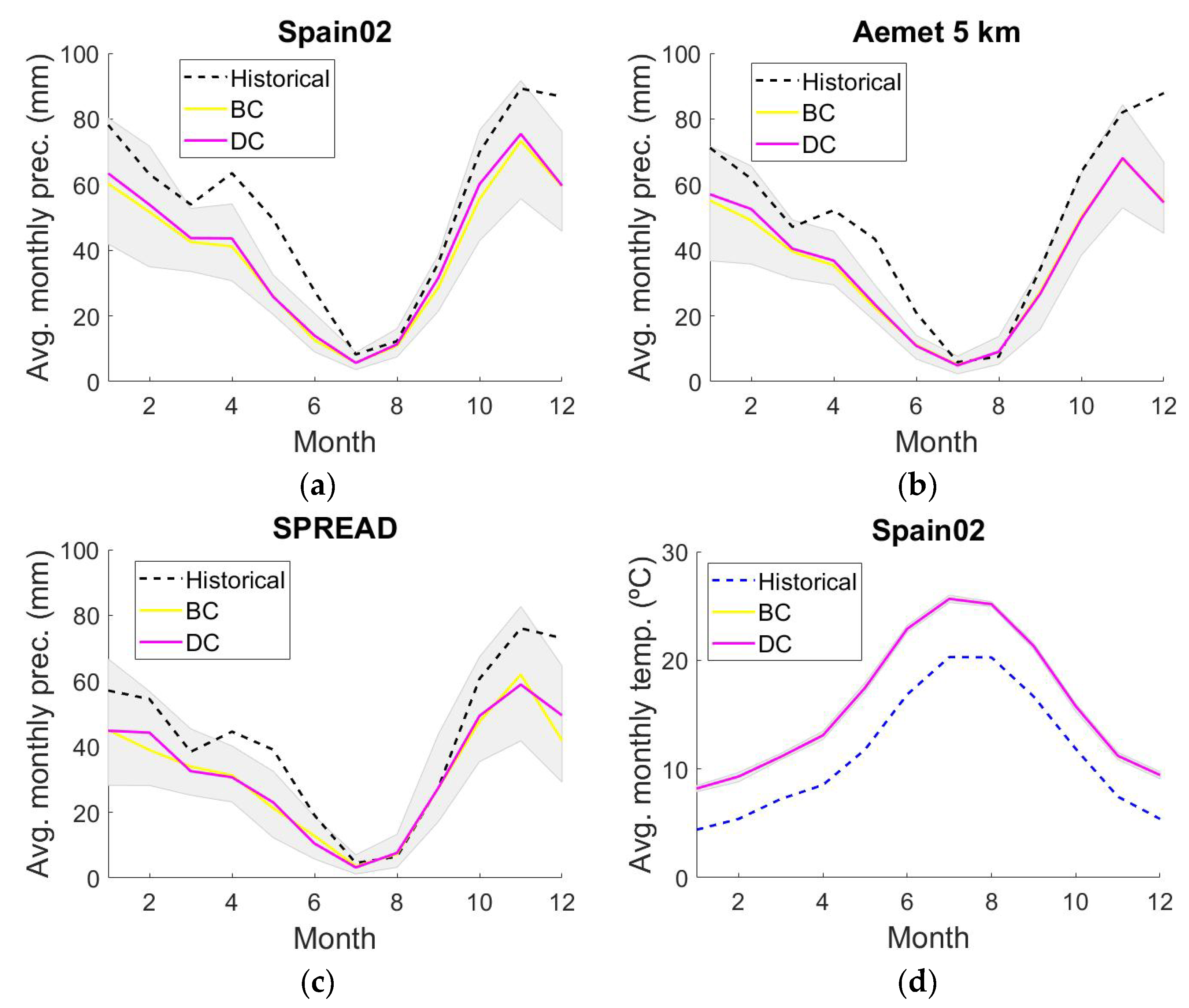
3.1. Assessment of the Meteorological (P and T) and Hydrological (SCA) Droughts

3.1.1. Historical Analysis

Figure 5 shows SPI and SPEI evolution for 3-, 6-, and 12-months temporal-aggregation scales during the historical period 1976–2005 in the study area. Shorter temporal-aggregation scales (e.g., 3 months) showed more frequent dry and wet period fluctuations. For higher temporal-aggregation scales (e.g., 12 months), dry and humid periods showed longer but less frequent fluctuations over time. The indices exhibited a similar trend without any notable differences, though it is worth mentioning more accentuated drought period detection with SPI, especially for smaller temporal-aggregation scales (3 months). With higher temporal-aggregation scales (12 months), the influence of evapotranspiration on droughts becomes more relevant.
SPI and SPEI series showed a similar temporal evolution, which indicates the high correlation between both indices. In order to compare the meteorological drought indices used, we analyzed the correlation between SPI and SPEI. Figure 6 shows the determination coefficient between both meteorological drought indices (SPI and SPEI) for the different temporal-aggregation scales (3, 6, and 12 months). The linear correlation coefficient calculated between SPI and SPEI ranged from 0.82 to 0.91. The lowest correlations were detected with the lowest temporal-aggregation scales (3 months) for all the climate databases. These correlations increased for the higher temporal-aggregation scale, obtaining the best results for the highest temporal-aggregation scale (12 months). It is important to note that SPEI and SPI have different minimum values (see the horizontal patterns of the data points in Figure 6a–c,e,f). However, the maximum values are similar.
A comparative analysis of meteorological droughts characteristics identifies similar results between climate databases (see Figure 7, Figure 8 and Figure 9) but shows significant differences between SPI and SPEI. SPI-3 shows more extreme events and severe droughts (20) than SPEI-3 (0) since the latter only identifies moderate and slight droughts (see Figure 7g, Figure 8g, and Figure 9g). The mean duration of the drought events detected with SPEI-3 was the longest (5 months) compared with SPI-3, which detects more intense and short droughts periods (2 months). The mean magnitude of SPI-3 and SPEI-3 shows a similar difference (−3.6 versus −4.2). Higher SPEI orders show a downward trend, with drought events that tend to be more severe. SPEI-12 detects events with similar intensity to those identified with SPI-12 (−1.9 vs. −2 on average) (see Appendix BFigure A5d,h, Figure A6d,h, and Figure A7d,h). The difference in the mean duration of drought events detected with SPEI-12 versus SPI-12 is notable (12 versus 9 months); however, for severe and extreme drought events, they average a similar duration (4 months). SPI-12 detects a higher number of events than SPEI-12 (21 vs. 15) but identifies the same frequency of severe drought events (5). In magnitude terms, the differences between SPI-12 and SPEI-12 are notable (−6.5 vs. −10). Magnitude is a drought severity indicator, so the SPEI provides more severe droughts than SPI (see Appendix BFigure A5c,g, Figure A6c,g and Figure A7c,g).
Likewise, we analyzed hydrological drought (SCA) characteristics in the Sierra Nevada mountain range. A statistical analysis shows significant differences in drought frequency, duration, and magnitude for the different temporal-aggregation scales, but no changes were detected in intensity. Lower SSCI values showed greater fluctuations than higher SSCI values, which show a lesser trend with prolonged dry periods. The number of drought events identified with SSCI-3 was higher (25) than that detected with SSCI-12 (15). However, SSCI-12 showed longer drought events (11 months) compared to those obtained with SSCI-3 (5 months). In the same way, the magnitude exhibited by SSCI-12 (−9) far exceeded that identified with SSCI-3 (−4,6) (see Figure 10 and Appendix BFigure A8).

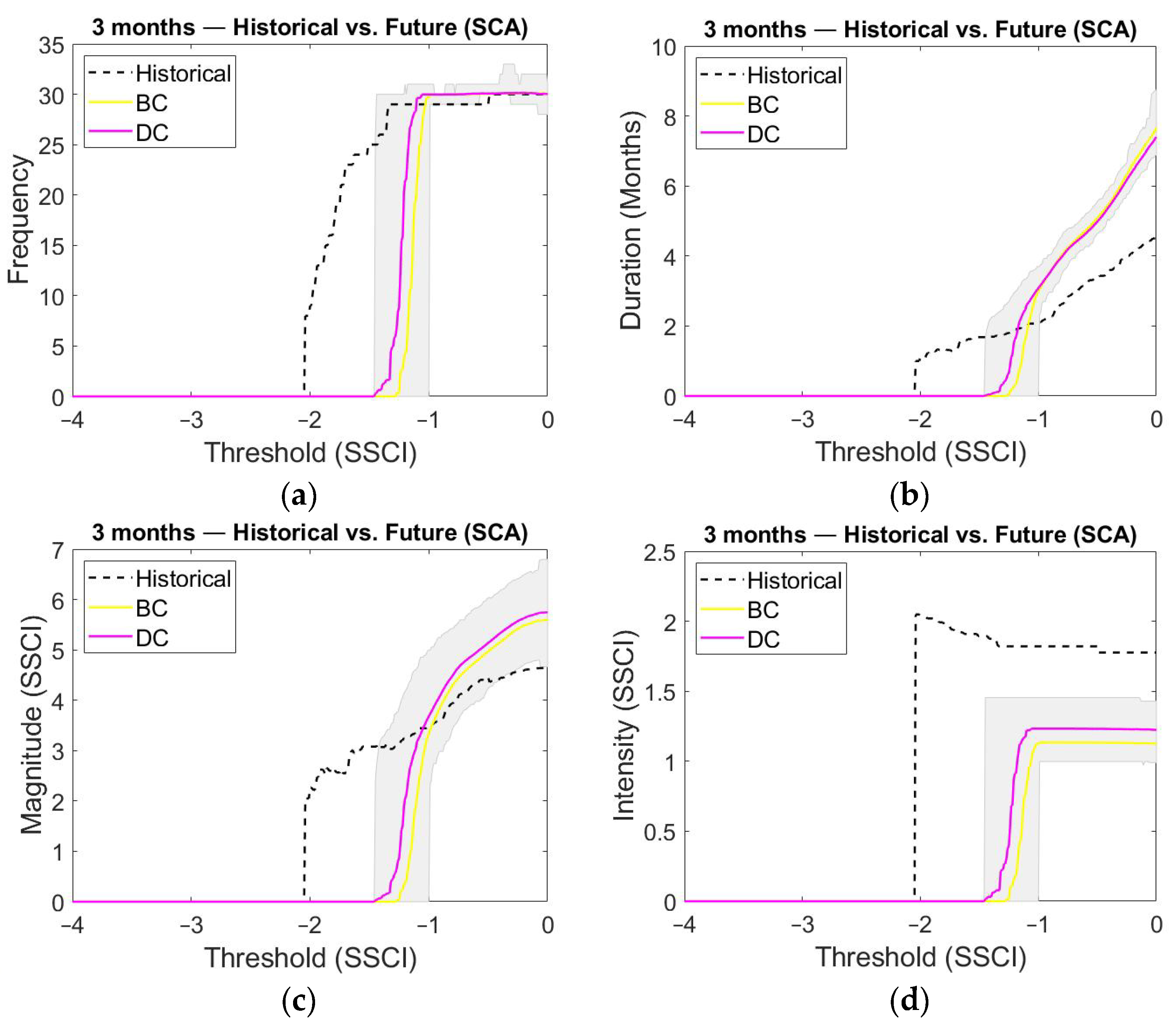
3.1.2. Future Analysis

Climate projections under RCP 8.5 emission scenarios based on different correction approaches (BC and DC) predict a significant reduction in precipitation (27–22% on average) for the 2071–2100 time horizon, with average precipitation varying between 373 to 468 mm year−1 and 381 to 488 mm year−1 for BC and DC approaches, respectively. The future mean precipitation differs depending on the climate database used. The Spain02 climate tool provides the highest mean precipitation values (468 to 488 mm year−1) (see Figure 11a), and the SPREAD database averages the lowest values (373 to 381 mm year−1) (see Figure 11c). The Aemet 5 km climate tool is in an intermediate range, it provides future precipitation values that vary on average from 427 to 434 mm year−1 for the BC and DC approaches, respectively (see Figure 11b). Regarding temperature, a considerable increase is predicted, which on average stands at 4.5 °C (for the BC and DC approaches) in relation to the historical period for all climate tools (see Figure 11d,e,f). It is important to note that the BC and DC generated temperature series have the same mean monthly values, but the series are different. Therefore, both approaches predict the same changes in mean temperatures when the same historical information is used. However, with each climate database, the predictions showed different mean temperatures for the mean year in the future. It is important to note that the historical series of the different databases are different. The mean temperatures predicted vary from 14.3 to 16.1 °C for the BC and DC approaches, respectively. The STEAD database predicted the highest mean temperatures (16.1 °C), whilst the Aemet 5 km climate tool predicted the lowest mean values (14.3 °C). The predictions made with the Spain02 database are in an intermediate range, with 15.9 °C mean temperature values. In alpine systems, another relevant aspect related to climate conditions is SCA. Maximum SCA annual periods in the 1976–2005 historical period are reached in winter months (January and February), with 449 and 439 km2 covered by snow, respectively. On the contrary, in summer (July and August), the SCA is practically nil (see Figure 11g). Future projections of SCA for the BC and DC approaches predict a significant reduction in annual SCA for the 2071–2100 future period, with a reduction in snow season of 2 months (May to October) with 195 and 176 km2 and 227 and 209 km2 maximum values in January and February for the BC and DC approaches, respectively (see Figure 11g). This represents an average annual SCA reduction from 79% and 75% for the BC and DC approaches, respectively, whilst in peak months (January and February), a reduction of 57% and 49% in January and 59% and 52% in February is predicted for the BC and DC approaches.
Variations in climate conditions and SCA dynamics have a determining effect on future meteorological and hydrological droughts. Under an RCP 8.5 emission scenario, meteorological drought showed a significantly increasing trend in the study area with all the climate tools. SPI-3 suffered an increase in the mean number of severe drought events for the Spain02 (27 vs. 21) and Aemet 5 km (22 vs. 18) climate databases compared to the observed period (see Figure 7a and Figure 8a). Severe drought duration showed a similar contrast with the historical one for SPI-3, but we observed a generalized increase in duration for Spain02 (7 versus 4 months) (see Figure 7b), Aemet 5 km (6 vs. 4 months) (see Figure 8b), and SPREAD (6 vs. 4 months) climate products (see Figure 9b). Likewise, we identified an increase in drought severity in relation to the observed period for Spain02 (−6.5 vs.−3.6) (see Figure 7c), Aemet 5 km (−5.5 vs. −3.6) (see Figure 8c), and SPREAD (−5.5 vs. −3.7) climate products (see Figure 9c). In contrast, no significant variation in drought intensity is detected in the future in any database. Statistical studies with SPEI-3 do not reveal significant changes in the number of drought events detected in the future, except for the analysis with the SPREAD and STEAD climate tool, which shows a lower number of drought episodes compared to the reference period (34 vs. 43) (see Figure 9e). However, the duration of drought events identified with SPEI-3 was much higher than that observed in the historical period with Spain02 (9 vs. 5 months) (see Figure 7f), Aemet 5 km (9 vs. 5 months) (see Figure 8f), and SPREAD and STEAD (9 vs. 5 months) (see Figure 9f) climate databases. In the same way, the magnitude of the droughts is accentuated with all the climate tools . However, there are no significant changes in drought intensity for all climate products (see Figure 7h, Figure 8h and Figure 9h).
In the long term, both SPI and SPEI show a considerable increase in the number of extreme and severe droughts detected in relation to the observed period. We also predicted an increase in drought duration. For example, the results obtained on average with respect to the observed period with Spain02 (82 vs. 8 months for SPI-12 and 131 vs. 10 months for SPEI-12), Aemet 5 km (74 vs. 8 months for SPI-12 and 196 vs. 10 months for SPEI-12), and SPREAD and STEAD (74 vs. 10 months for SPI-12 and 196 vs. 17 months for SPEI-12) climate products, with drought events that were longer for scenarios generated with the BC approaches. Future drought severity (2071–2100) shows mean magnitudes that far exceeded the values identified in the reference period (1976–2005) for Spain02 (−100.2 vs. −5.9 for SPI-12 and −206.9 vs. −7.8 for SPEI-12), Aemet 5 km (−74.1 vs. −6 for SPI-12 and −272.6 vs. −8 for SPEI-12), and SPREAD and STEAD (−74.1 vs. −7.6 for SPI-12 and −272.7 vs. −14.2 for SPEI-12) databases. Likewise, we revealed more intense droughts for the RCP 8.5 emission scenario with SPI-12 and SPEI-12 in all climate databases (see Appendix BFigure A5, Figure A6, and Figure A7).
Hydrological drought statistics for the 3-month temporal-aggregation scale can be seen in Figure 10. Hydrological droughts at lower temporal-aggregation scales (3 months) showed less extreme and severe drought events, with SSCI values that never exceed the −1.5 barrier in the future. Predictions revealed that there was no variation in the number of drought events compared to the reference period, but there was a notable increase in the duration of these events (8 months for the BC approach and 7 months for the DC approach, vs. 5 months). Drought magnitude showed similar differences (−5.6 and −5.7 for the BC and DC approaches, respectively, vs. −4.6), which is due to the remarkable reduction that was observed in the mean drought intensity (−1.2 for BC and DC approaches vs. −1.8). These results contrast with those obtained for the higher temporal-aggregation scale, with droughts that were much more intense in the future (−6.2 for the BC approach and −5.8 for the DC approach vs. −2.1). Future predictions for hydrological SCA droughts showed a continuous extreme drought time period in the Sierra Nevada with the BC approach, with a single drought event for the entire analyzed period (349 months). Similar results were revealed with the DC approach, with a single extreme drought event that lasted most of the study time period (303 months). Drought magnitude was much higher (−1436.6 for the BC approach and −1269.6 for the DC approach, vs. −8.9) compared to the reference period (see Appendix BFigure A8).

3.1.3. Assessment of the Correlations between Meteorological (P and T) and Hydrological (SCA) Droughts

We analyzed the linear correlation between multiple meteorological (SPI and SPI) drought indices and the hydrological (SSCI) drought index series (generated with BC and DC correction approaches). The mean values of these correlations for the BC and DC approaches are shown in Figure 12. The snow dynamics response to meteorological conditions was identified with a 0 to 3 months’ time lag (see Figure 12). In general, snow depends on climate characteristics (temperature and relative humidity). The highest correlation values occurred for smaller temporal-aggregation scales (3 and 6 months) with short response times (0 to 1 month). In general, correlations decreased significantly on the longest time aggregation scale (12 months). It should be noted that correlation was slightly higher with SPEI. In particular, from the climate databases used, it should be noted that the meteorological drought series produced with Spain02 had a higher correlation with the hydrological drought series (SSCI). For drought propagation, the 1 month response time seems to be a turning point in all the temporal-aggregation scales. The highest correlation in the reference period 1976–2005 (0.63) occurred in the 3-month temporal-aggregation scale with an immediate response time (0 months). Thus, this indicates that the corresponding month’s climate condition was the most significant variable that contributed to the SCA dynamics in Sierra Nevada.
In general, the SPI mean correlations with SSCI are higher in the future, especially in the lower temporal-aggregation scales. In contrast, the SPEI shows slightly lower correlations with the SSCI. However, the maximum mean correlation took place with the SPEI in 3-month temporal-aggregation scale with no delay in hydrological drought response, with a 0.69 value for the Spain02 climate tool. In contrast, the highest SPI mean correlation (0.66) occurred with a 1 month time lag.

4. Discussion

Climate models provide essential information to study the impact of climate change on droughts. However, there is high uncertainty in scenarios generated from GCM and RCM simulations that may cause a drought persistence underestimation [77]; therefore, an uncertainties analysis associated with climate models must be incorporated. One way to reduce this uncertainty in the climate projections is to merge multiple RCMs, which provide more robust results than individual models [49]. SWGs are useful tools to take into account uncertainty by generating equi-probable multiple weather series preserving the values identified in some statistics for the future climate. SWG has been used extensively in previous studies to assess the impact of climate change [78,79]. In this study, we used an SWG to quantify the climate change uncertainty in meteorological and hydrological droughts associated with SCA.
Most studies have used standardized indices with multi-scale properties, comparable in time and space, for drought analysis and monitoring [80,81,82]. In our study, we used SPI and SPEI indices for meteorological droughts and a novel variant of the SPI (SSCI) for hydrological droughts to assess the impact of climate change (and its uncertainty) on multiple time scales. These indices require continuous climate records (precipitation and temperature) over a long enough time period. Climate tools contain continuous climate records (precipitation and temperature) over a long period of time with a fixed spatial scale and are useful in areas where data are scarce (such as alpine areas). In this study, we used the climate products available in Peninsular Spain (Spain02, Aemet 5 km, and SPREAD and STEAD). Other researchers have analyzed the impact of climate change (and its uncertainty) on droughts in other regions [83,84], but not in the Sierra Nevada mountain range. Nevertheless, the methodology applied in this study is a parsimonious approach applicable to any case study. Only historical SCA and climate data and future RCM and SCA climate data are needed to assess the impact of climate change (and its uncertainty) on meteorological and hydrological droughts.
Drought characteristics (including frequency, duration, magnitude, and intensity) have an implicit or explicit relationship with the established temporal-aggregation scale. In general, long temporal-aggregation scale indices are more likely to indicate moderate droughts that persist for long periods of time, whilst short temporal-aggregation scales indicate more severe droughts with short durations [85]. In this article, behavior analysis of each temporal-aggregation scale in meteorological and hydrological drought detection in the reference period agrees with the above observation. Results in the reference period (1976–2005) revealed high correlations between SPI and SPEI in each temporal-aggregation scale, which indicates that precipitation variability is the main meteorological drought driver. For the 1976–2005 historical period, the meteorological droughts studied with SPEI identified more serious droughts that manifested for a longer time compared to those detected with SPI in each temporal-aggregation scale, which shows the importance of considering potential evapotranspiration in drought analysis. However, despite what we might expect, the most intense droughts were detected with SPI. Although most research refers to the greater capacity of SPEI to identify droughts [86,87], there is no common agreement regarding the severity detected. In some studies in semi-arid regions, higher intensities were detected with SPI [88,89,90], whilst in others, a higher severity was always identified with SPEI [91]. Other investigations showed more extreme droughts with SPI at lower temporal-aggregation scales, although similar or even slightly higher intensities were identified in higher accumulation periods with SPEI [92]. In this study, although the droughts were generally more extreme with SPI, we only identified slightly more severe droughts with SPEI at longer temporal-aggregation scales. These results are consistent with other investigations in the Mediterranean region [66,93], where precipitation variability controls drought occurrence.
For the 2071–2100 horizon under the RCP 8.5 emission scenario, climate change’s impact on meteorological droughts in Sierra Nevada is very significant. Future scenarios indicate a reduction in precipitation from 22 to 27% and a 4.5 °C increase in average temperature at the end of the 21st century, which is consistent with other studies that evaluated climate change impact in the Mediterranean region [94,95]. This notable alteration in future climate conditions explains the significant impact on droughts. Despite relevant uncertainty, we expected a general increase in drought severity and duration. Future drought scenarios based on SPI showed less significant changes compared to SPEI. When considering the temperature effect, SPEI-based scenarios show a clear trend towards drastically more severe and prolonged droughts. However, both SPI and SPEI detected considerable deviations from normal conditions in the reference period. Several studies that used SPI and SPEI indices to assess the impact of climate change on meteorological drought in semi-arid regions reached the same conclusions [66,96]. These results demonstrate that temperature is the dominant factor contributing to increased drought compared to other factors such as precipitation. The importance of considering potential evapotranspiration in drought analysis under global warming scenarios has been highlighted in previous studies [23], thus demonstrating the consistency of our results.
SCA analysis in RCP 8.5 (the higher emission scenario) revealed a very considerable impact on hydrological droughts. During winter (December to March), we expected reductions from 46 to 66% in SCA, although further reductions are expected in the rest of the year. This significant impact on SCA has a direct effect on hydrological droughts, with a general increase in drought magnitude, severity, and duration. Other studies have also demonstrated the significant impact of climate change on SCA in other mountain ranges [97,98,99]; however, there are no studies that have evaluated the impact of climate change on SCA droughts.
We also analyzed the correlation of SSCI with the SPI and SPEI using a linear regression model for the different accumulation periods to identify the temporal-aggregation scale in which precipitation and effective precipitation deficits propagate through hydrological cycles to produce deficits in SCA. Another possible option would be to use the cross-wavelet analysis, which is a robust method that shows how the components of the time series are coherent in the time-frequency domain and provides phase lag information. The cross-wavelet analysis has been used in other research to study the coherency between the seasonal components of climate and vegetation time series and provide the phase lag [100,101], and investigate the relationship between the climate indices and drought/flood conditions [102,103], amongst others. In this study, the precipitation SCA relationship reflects an important correlation coefficient between meteorological and hydrological droughts. The SSCI series revealed a good correlation with SPI and SPEI series in lower temporal-aggregation scales (3 and 6 months), but we observed a considerable reduction in the relationship for the 12-month temporal-aggregation scale. The SPEI series showed a higher correlation with the SSCI series, which shows the effect of temperature on SCA dynamics. Other researchers have identified the influence of climate variables on the snow dynamics in the Sierra Nevada [13,14]. These studies identified the precipitation regime as the main snow dynamics driver, not underestimating the influence of temperature. Correlations between meteorological and hydrological droughts show good correlations for short response times in the different SPI and SPEI accumulation periods. Although the strongest correlation occurs when SPEI is not lagged, the presence of weak correlations in time lags of several months demonstrates the lack of early warning potential for hydrological droughts based on the persistence of meteorological anomalies.

5. Conclusions

We proposed a methodology to evaluate the potential impact of climate change (and its uncertainty) for meteorological and hydrological droughts. We generated local ensemble scenarios from RCMs by combining the results obtained with different statistical downscaling techniques under BC and DC approaches. We applied an SWG to generate multiple series based on the generated ensemble of local scenarios. Relative standardized indices were used to assess the impact of climate change on meteorological (SPI and SPEI) and hydrological (SSCI) droughts at different time scales. We analyzed drought frequency, duration, magnitude, and intensity trends to better understand temporal changes in drought characteristics.
The methodology used in this study is applicable to any case study. We applied it to the Sierra Nevada mountain range, which is an alpine area highly sensitive to climate change. For the most pessimistic emission scenario, RCP 8.5, we estimated a reduction from 27 to 22% in precipitation and an increase in temperature of 4.5 °C at the end of the 21st century, which will affect SCA dynamics, with a reduction of 2 months for the snow season in and an average reduction from 79 to 75% in the annual SCA. Meteorological drought analysis revealed the usefulness of SPEI evaluating drought characteristics in climate change scenarios due to the fundamental role of temperature in potential evapotranspiration. Despite relevant uncertainty, our results showed that climate change scenarios lead to a generalized increase in both meteorological and hydrological drought statistics, with a considerable effect on duration (174 versus 12 months for meteorological droughts and 326 vs. 11 months for hydrological drought) and magnitude (−250 vs. −7 for meteorological drought and −1353 vs. −9 for hydrological drought) in the long-term drought study in relation to the reference period. Although in the historical period, the SPI shows similar values to SPEI, under climate change scenarios, the SPI could underestimate drought magnitude and duration.
The correlation between meteorological and hydrological droughts provides a better understanding of drought propagation procedures and can provide early warning to identify potential adaptation strategies. In this study, we applied a linear regression model to detect the multiple-scale relationship between meteorological and hydrological droughts. Correlation analysis demonstrated a good hydrological response to precipitation and/or effective precipitation deficits at short temporal-aggregation scales, although for long temporal-aggregation scales, the hydrological response was weaker. The propagation time from meteorological to hydrological drought presents stable characteristics in multiple temporal-aggregation scales, with an immediate or short response time (1 month).

Author Contributions

D.P.-V. and F.J.R. conceived and designed the research; A.-J.C.-L. conceived and designed the research and analyzed the data (generating local future scenarios); J.-D.H.-H. analyzed the data and conducted the experiments; E.P.-I. designed the cellular automata model that provided the snow cover data. All authors have read and agreed to the published version of the manuscript.

Funding

This research was partially supported by the research project SIGLO-AN (RTI2018-101397-B-I00) from the Spanish Ministry of Science, Innovation and Universities (Programa Estatal de ICDCI orientado a los Retos de la Sociedad), the GeoE.171.008.TACTIC from the GeoERA organization funded by European Union’s Horizon 2020 research and innovation program and the Regional Ministry of Economic Transformation, Industry, Knowledge and Universities of the Regional Government of Andalusia through the postdoc program of the Andalusian Plan for Research Development and Innovation (PAIDI 2021) (POSTDOC_21_00154, University of Granada, Antonio-Juan Collados-Lara).

Institutional Review Board Statement

Not applicable.

Informed Consent Statement

Not applicable.

Data Availability Statement

Not applicable.

Acknowledgments

We would like to thank the Spain02, Aemet 5 km, SPREAD, STEAD, and CORDEX projects for the data provided for this study. The work of the first author at “Instituto Geológico y Minero de España” was conducted within the internship program of the Master in Water Quality Science and Technology (University of Granada).

Conflicts of Interest

The authors declare no conflict of interest.

Abbreviations

BCBias correction.
CACellular automata.
DCDelta change.
GCMGlobal climate model.
MAGRAMAAgriculture and Environmental Ministry.
MODISModerate Resolution Imaging Spectroradiometer.
NOAANational Oceanic and Atmospheric Administration.
PAGEPrecipitation Altitudinal Gradient with Elevation.
RCMRegional Climate Model.
SCASnow cover area.
SPEIStandardized Precipitation Evapotranspiration Index.
SPIStandardized Precipitation Index.
SSCIStandardized Snow Cover Index.
SWGStochastic Weather Generator.
TAGETemperature Altitudinal Gradient with Elevation.

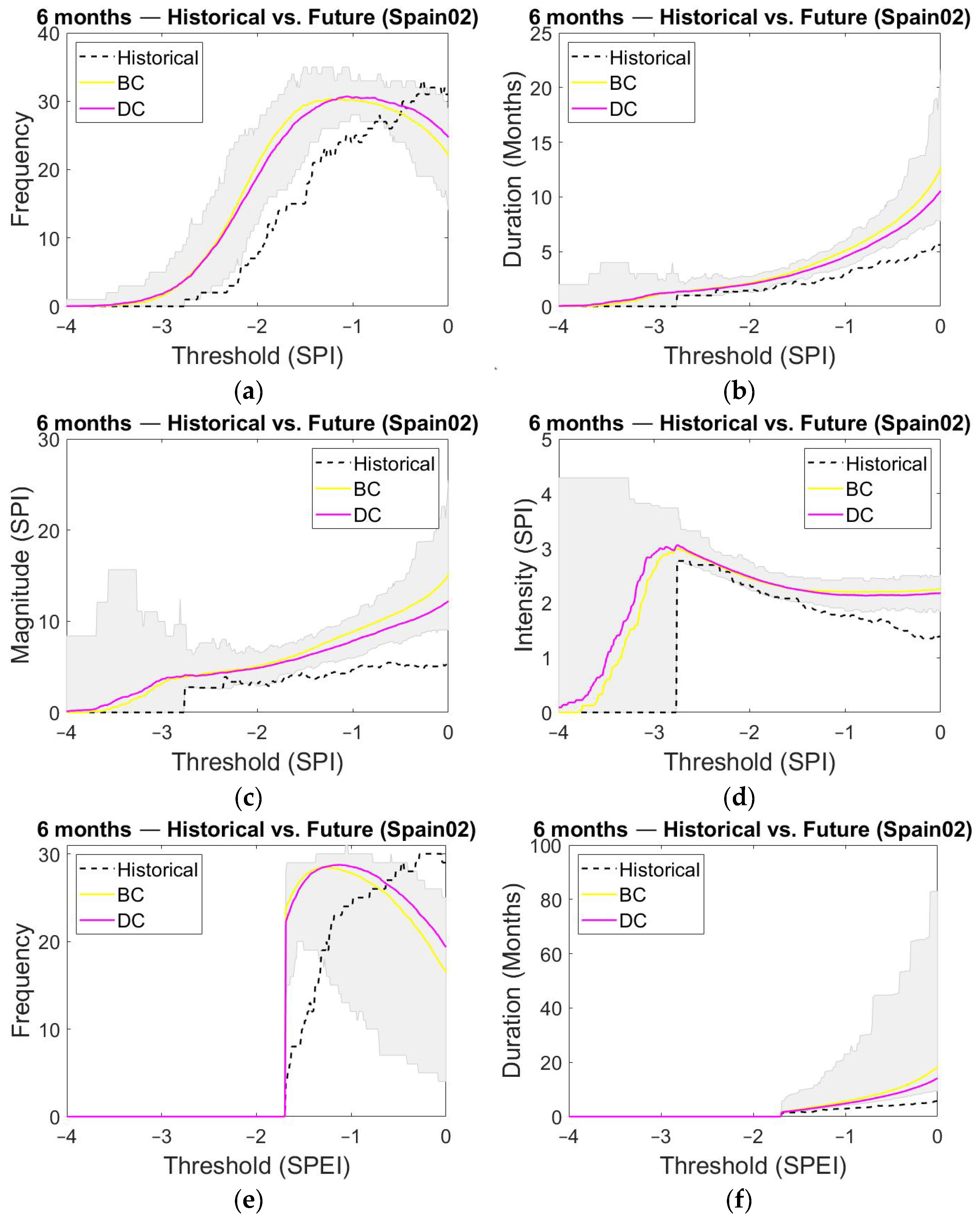
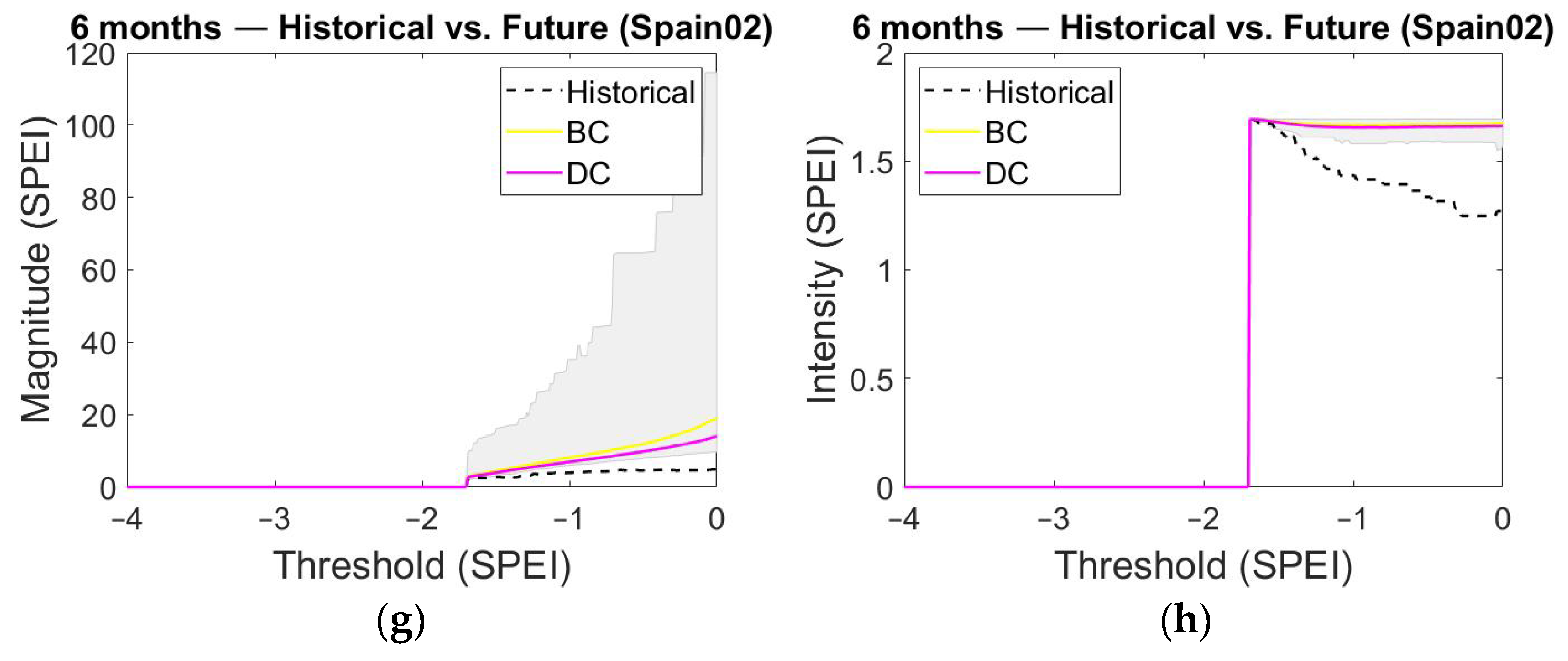
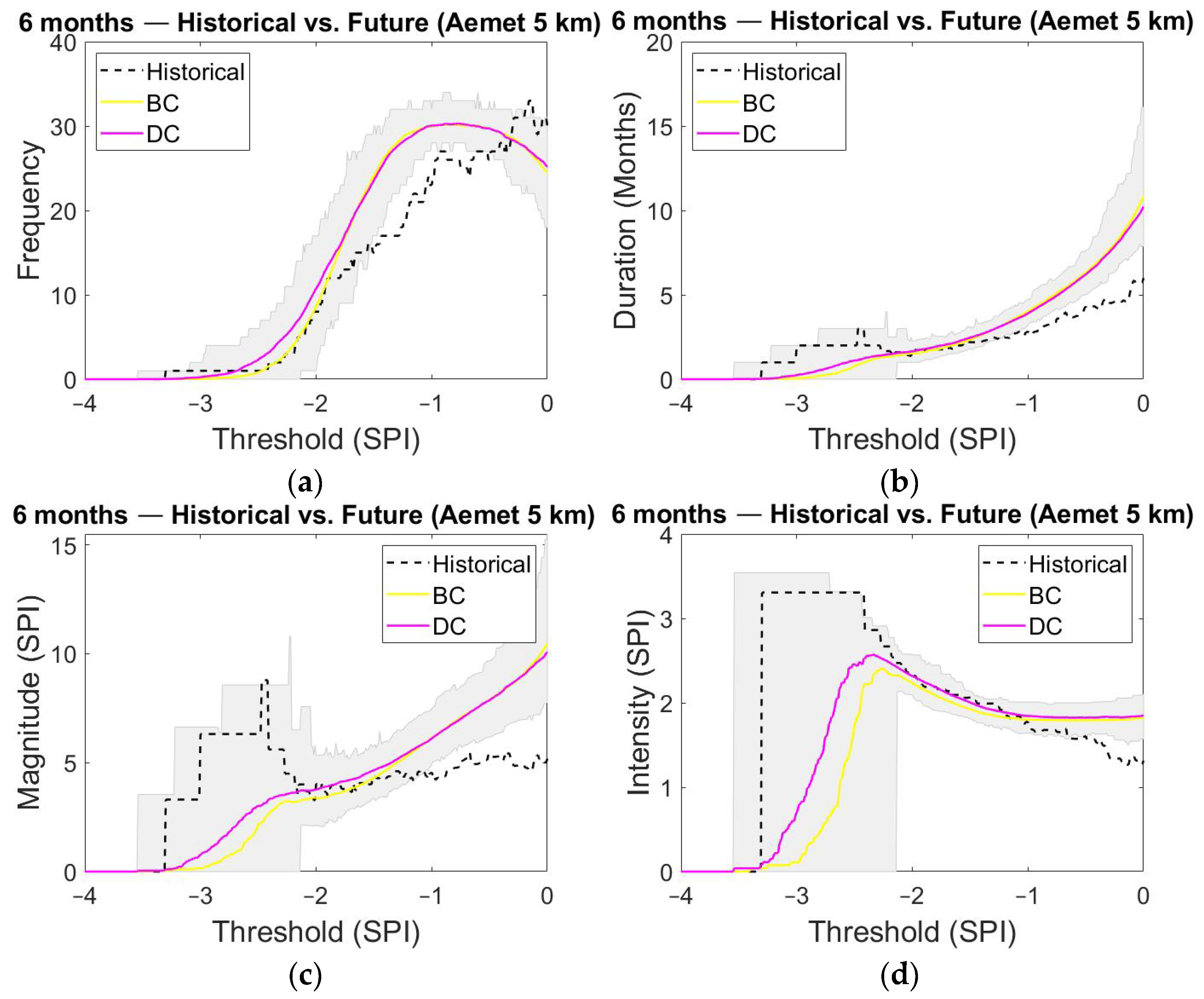
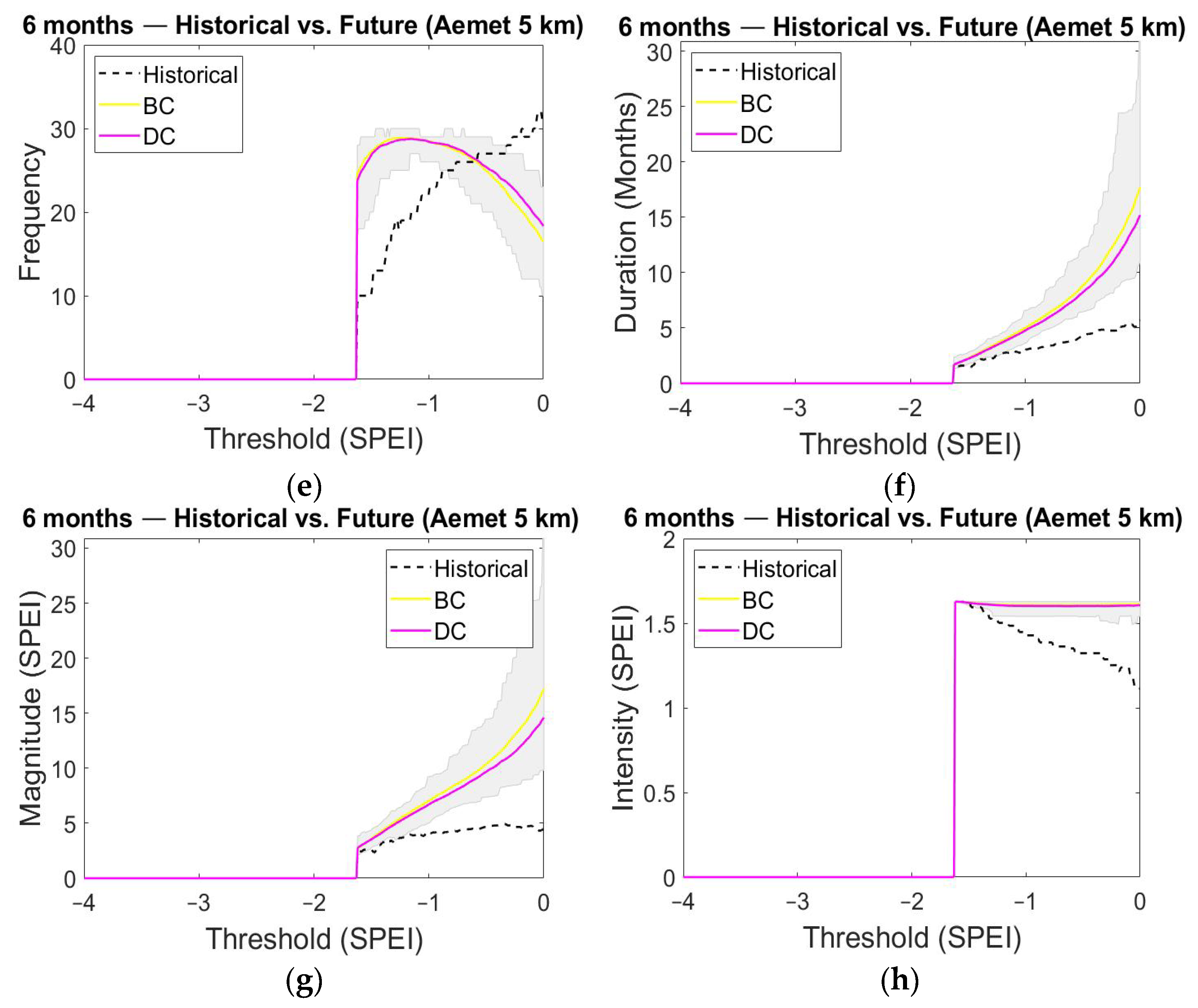
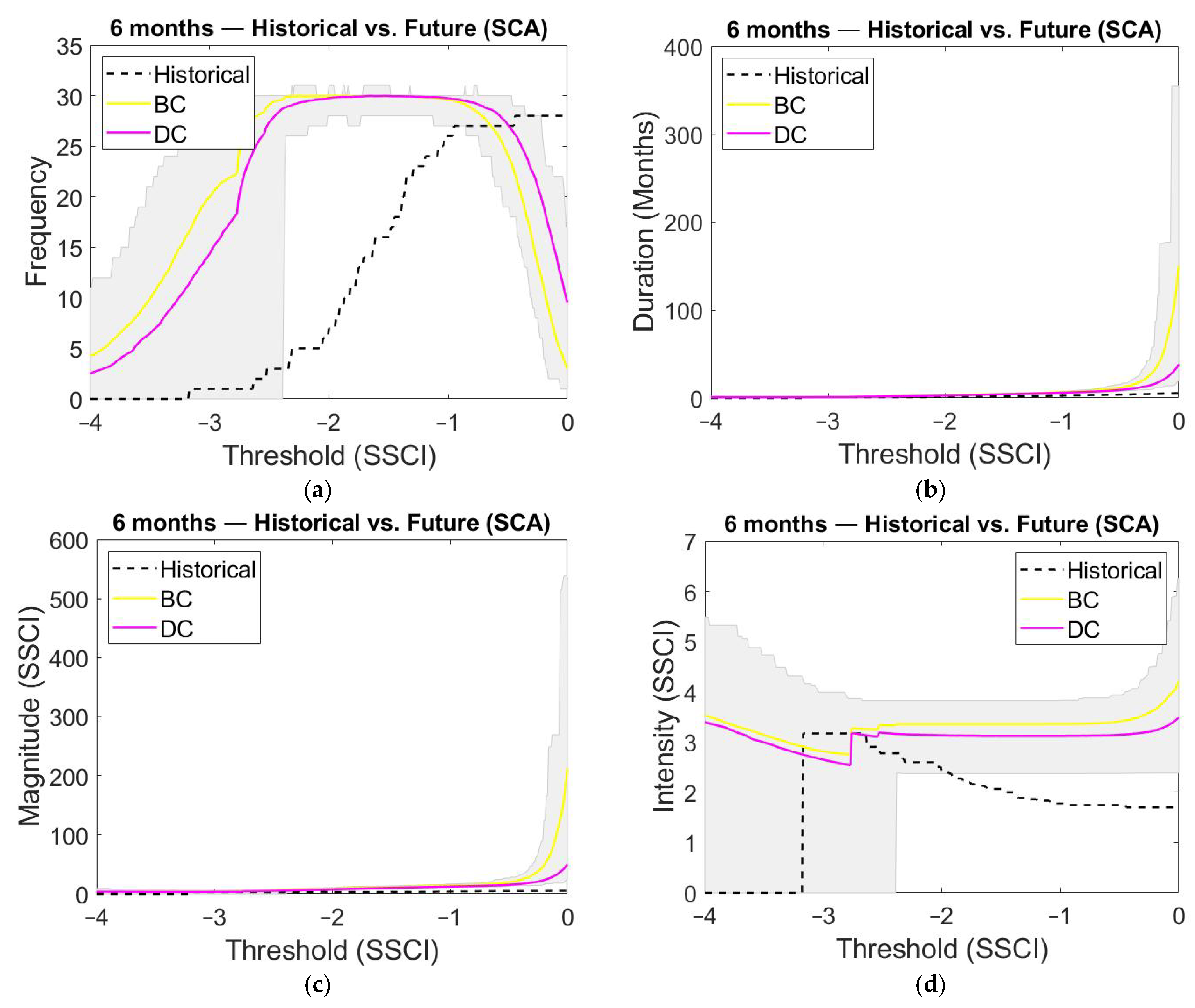
Appendix A. Drought Statistics for the 6-Month Time-Aggregation Scale

Figure A1. Historical and future meteorological drought (a) frequency; (b) mean duration; (c) mean magnitude; (d) mean intensity derived from SPI for the 6 months temporal-aggregation scale (Spain02 database). Historical and future meteorological drought (e) frequency; (f) mean duration; (g) mean magnitude; (h) mean intensity derived from SPEI for the 6 months temporal-aggregation scale (Spain02 database).
Water 14 01081 g0a1aWater 14 01081 g0a1b
Figure A2. Historical and future meteorological drought (a) frequency; (b) mean duration; (c) mean magnitude; (d) mean intensity derived from SPI for the 6 months temporal-aggregation scale (Aemet 5 km database). Historical and future meteorological drought (e) frequency; (f) mean duration; (g) mean magnitude; (h) mean intensity derived from SPEI for the 6 months temporal-aggregation scale (Aemet 5 km database).
Water 14 01081 g0a2aWater 14 01081 g0a2b
Figure A3. Historical and future meteorological drought (a) frequency; (b) mean duration; (c) mean magnitude; (d) mean intensity derived from SPI for the 6 months temporal-aggregation scale (SPREAD and STEAD database). Historical and future meteorological drought (e) frequency; (f) mean duration; (g) mean magnitude; (h) mean intensity derived from SPEI for the 6 months temporal-aggregation scale (SPREAD and STEAD database).
Water 14 01081 g0a3aWater 14 01081 g0a3b
Figure A4. Historical and future hydrological drought (a) frequency; (b) mean duration; (c) mean magnitude; (d) mean intensity derived from SSCI for the 6 months temporal-aggregation scale.
Water 14 01081 g0a4

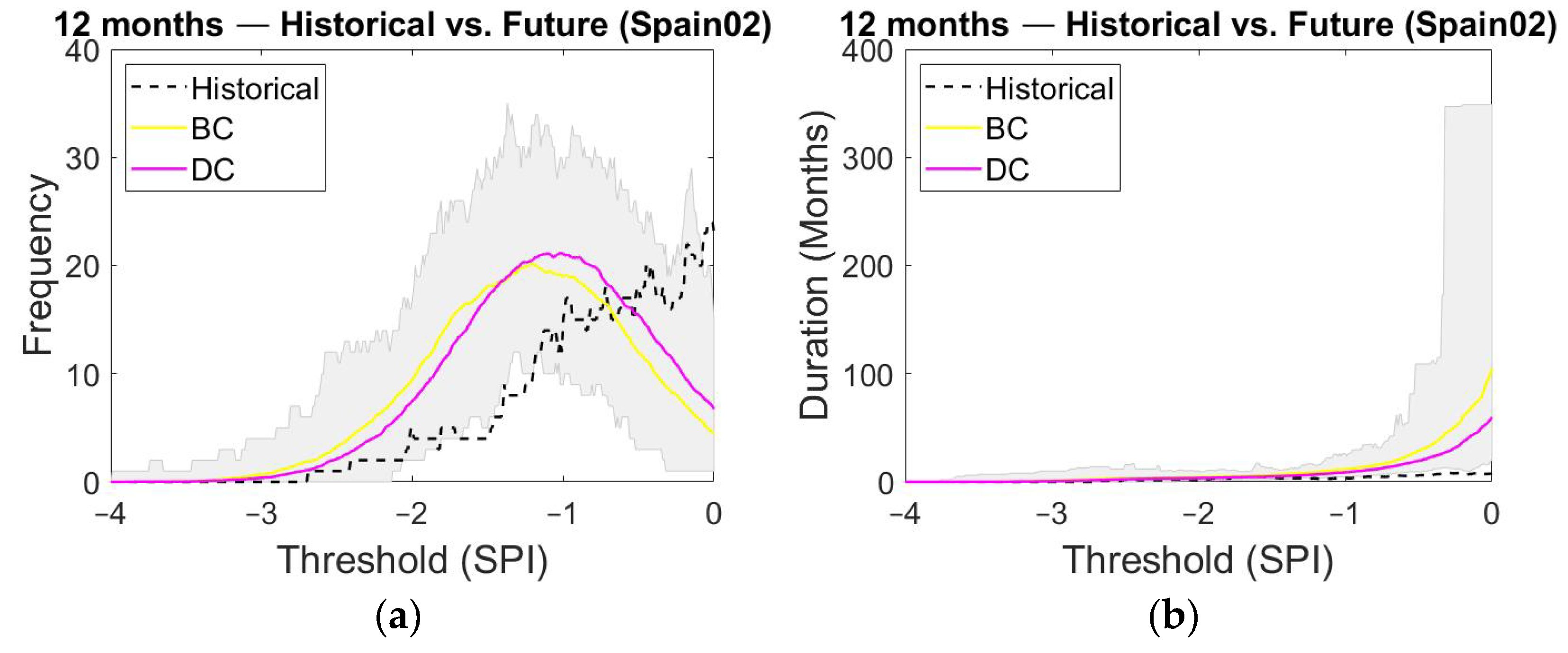
Appendix B. Drought Statistics for the 12-Month Time Aggregation Scale

Figure A5. Historical and future meteorological drought (a) frequency; (b) mean duration; (c) mean magnitude; (d) mean intensity derived from SPI for the 12 months temporal-aggregation scale (Spain02 database). Historical and future meteorological drought (e) frequency; (f) mean duration; (g) mean magnitude; (h) mean intensity derived from SPEI for the 12 months temporal-aggregation scale (Spain02 database).
Water 14 01081 g0a5aWater 14 01081 g0a5b
Figure A6. Historical and future meteorological drought (a) frequency; (b) mean duration; (c) mean magnitude; (d) mean intensity derived from SPI for the 12 months temporal-aggregation scale (Aemet 5 km database). Historical and future meteorological drought (e) frequency; (f) mean duration; (g) mean magnitude; (h) mean intensity derived from SPEI for the 12 months temporal-aggregation scale (Aemet 5 km database).
Water 14 01081 g0a6
Figure A7. Historical and future meteorological drought (a) frequency; (b) mean duration; (c) mean magnitude; (d) mean intensity derived from SPI for the 12 months temporal-aggregation scale (SPREAD and STEAD database). Historical and future meteorological drought (e) frequency; (f) mean duration; (g) mean magnitude; (h) mean intensity derived from SPEI for the 12 months temporal-aggregation scale (SPREAD and STEAD database).
Water 14 01081 g0a7
Figure A8. Historical and future hydrological drought (a) frequency; (b) mean duration; (c) mean magnitude; (d) mean intensity derived from SSCI for the 12 months temporal-aggregation scale.
Water 14 01081 g0a8

References

  1. Senet-Aparicio, J.; López-Ballesteros, A. Using Multiple Monthly Water Balance Models to Evaluate Gridded Precipitation Products over Peninsular Spain. Remote Sens. 2018, 10, 922. [Google Scholar] [CrossRef] [Green Version]
  2. Rood, S.B.; Pan, J.; Gill, K.M.; Franks, C.G.; Samuelson, G.M.; Shepherd, A. Declining summer flows of Rocky Mountain rivers: Changing seasonal hydrology and probable impacts on floodplain forests. J. Hydrol. 2008, 349, 397–410. [Google Scholar] [CrossRef]
  3. Tague, C.; Peng, H. The sensitivity of forest wáter use to the timing of precipitation and snowmelt recharge in the California Sierra: Implicaions for a warming climate. J. Geophys. Res. Biogeosci. 2013, 118, 875–887. [Google Scholar] [CrossRef]
  4. Barnett, T.P.; Pierce, D.W.; Hidalgo, H.G.; Bonfils, C.; Santer, B.D.; Das, T.; Bala, G.; Wood, A.W.; Nozawa, T.; Mirin, A.A.; et al. Human-Induced Changes in the Hydrology of the Western United States. Science 2008, 319, 1080–1083. [Google Scholar] [CrossRef] [Green Version]
  5. Taylor, R.G.; Scanlon, B.; Döll, P.; Rodell, M.; Van Beek, R.; Wada, Y.; Longuevergne, L.; Leblanc, M.; Famiglietti, J.S.; Edmunds, M.; et al. Ground water and climate change. Nat. Clim. Chang. 2013, 3, 322–329. [Google Scholar] [CrossRef] [Green Version]
  6. Hayhoe, K.; Cayan, D.; Field, C.B.; Frumhoff, P.C.; Maurer, E.P.; Miller, N.L.; Moser, S.C.; Schneider, S.H.; Cahill, K.N.; Cleland, E.E.; et al. Emissions pathways, climate change, and impacts on California. Proc. Natl. Acad. Sci. USA 2004, 101, 12422–12427. [Google Scholar] [CrossRef] [PubMed] [Green Version]
  7. Falk, M. A Dynamic panel data análisis of snow Depth and Winter tourism. Tour. Manag. 2009, 31, 912–924. [Google Scholar] [CrossRef]
  8. Fayad, A.; Gascoin, S.; Faour, G.; Lopez-Moreno, I.; Drapeau, L.; Le Page, M.; Escadafal, R. Snow hydrology in Mediterranean mountain regions: A review. J. Hydrol. 2017, 551, 374–396. [Google Scholar] [CrossRef]
  9. Collados-Lara, A.-J.; Fassnacht, S.; Pardo-Igúzquiza, E.; Pulido-Velazquez, D. Assessment of High Resolution Air Temperature Fields at Rocky Mountain National Park by Combining Scarce Point Measurements with Elevation and Remote Sensing Data. Remote Sens. 2020, 13, 113. [Google Scholar] [CrossRef]
  10. Collados-Lara, A.; Fassnacht, S.R.; Pulido-Velazquez, D.; Pfohl, A.K.; Morán-Tejeda, E.; Venable, N.B.; Pardo-Igúzquiza, E.; Puntenney-Desmond, K. Intra-day variability of temperature and its near-surface gradient with elevation over mountainous terrain: Comparing MODIS land surface temperature data with coarse and fine scale near-surface measurements. Int. J. Climatol. 2021, 41, 1435–1449. [Google Scholar] [CrossRef]
  11. Collados-Lara, A.J.; Pardo-Igúzquiza, E.; Pulido-Velazquez, D.; Jiménez-Sánchez, J. Precipitation fields in an alpine Mediterranean catchment. Inversion of precipitation gradient with elevation or undercatch of snowfall? Int. J. Hydrol. 2018, 38, 3565–3578. [Google Scholar] [CrossRef]
  12. Alonso-González, E.; López-Moreno, J.I.; Navarro-Serrano, F.; Sanmiguel-Vallelado, A.; Aznárez-Balta, M.; Revuelto, J.; Ceballos, A. Snowpack sensivity to temperature, precipitation, and solar radiation variability over an elevational gradient in the Iberian mountains. Atmos. Res. 2020, 243, 104973. [Google Scholar] [CrossRef]
  13. Pérez-Palazón, M.J.; Pimentel, R.; Herrero, J.; Aguilar, C.; Perales, J.M.; Polo, M.J. Extreme values of snow-related variables in Mediterranean regions: Trends and long-term forecasting in Sierra Nevada (Spain). Proc. Int. Assoc. Hydrol. Sci. 2015, 369, 157–162. [Google Scholar] [CrossRef] [Green Version]
  14. Jimeno-Sáez, P.; Pulido-Velazquez, D.; Collados-Lara, A.-J.; Pardo-Igúzquiza, E.; Senent-Aparicio, J.; Baena-Ruiz, L. A Preliminary Assessment of the Undercatching and the Precipitation Pattern in an Alpine Basin. Water 2020, 12, 1061. [Google Scholar] [CrossRef] [Green Version]
  15. Tramblay, Y.; Kautroulis, A.; Samaniego, L.; Vicente-Serrano, S.M.; Volaire, F.; Boone, A.; Le Page, M.; Llasath, M.C.; Albergel, C.; Burak, S.; et al. Challenges for drought assessment in the Mediterranean region under future climate scenarios. Earth-Sci. Rev. 2020, 210, 103348. [Google Scholar] [CrossRef]
  16. Pulido-Velázquez, D.; Romero, J.; Collados-Lara, A.J.; Alcalá, F.J.; Fernández-Chacón, F.; Baena-Ruiz, L. Using the Tumover Time Index to Identify Potential Strategic Groundwater Resources to Manage Droughts within Continental Spain. Water 2020, 12, 3281. [Google Scholar] [CrossRef]
  17. Gleick, P.H. Water and Conflict: Fresh Water Resources and International Security. Int. Secur. 1993, 18, 79. [Google Scholar] [CrossRef]
  18. Lloyd-Hughes, B. The impracticality of a universal drought definition. Theor. Appl. Climatol. 2014, 117, 607–611. [Google Scholar] [CrossRef] [Green Version]
  19. Sheffield, J.; Wood, E.F. Drought: Past Problems and Future Scenarios; Earthscan: London, UK, 2011; p. 11. [Google Scholar]
  20. Wilhite, D.A.; Glantz, M.H. Understanding: The Drought Phenomenon: The Role of Definitions. Water Int. 1985, 10, 111–120. [Google Scholar] [CrossRef] [Green Version]
  21. Kahil, M.T.; Dinar, A.; Albiac, J. Modeling water scarcity and droughts for policy adaptation to climate change in arid and semiarid regions. J. Hydrol. 2015, 522, 95–109. [Google Scholar] [CrossRef] [Green Version]
  22. McKee, T.B.; Doesken, N.J.; Kleist, J. The relationship of drought frequency and duration to time scales. In Proceedings of the 8th Conference on Applied Climatology, Boston, MA, USA, 17–22 January 1993; Voulme 17, pp. 179–183. [Google Scholar]
  23. Vicente-Serrano, S.M.; Beguería, S.; López-Moreno, J.I. A Multiscalar Drought Index Sensitive to Global Warming: The Standardized Precipitation Evapotranspiration Index. J. Clim. 2010, 23, 1696–1718. [Google Scholar] [CrossRef] [Green Version]
  24. Wu, H.; Hayes, M.J.; Wilhite, D.A.; Svoboda, M.D. The effect of the length of record on the standardized precipitation index calculation. Int. J. Climatol. 2005, 25, 505–520. [Google Scholar] [CrossRef] [Green Version]
  25. Parajka, J.; Holko, L.; Kostka, Z.; Blöschl, G. MODIS snow cover mapping accuracy in a small mountain catchment – Comparison between open and forest sites. Hydrol. Earth Syst. Sci. 2012, 16, 2365–2377. [Google Scholar] [CrossRef] [Green Version]
  26. Forysthe, N.; Fowler, H.J.; Kilsby, C.G.; Archer, D.R. Opportunities from Remote Sensing for Supporting Water Resources Management in Village/Valley Scale Catchments in the Upper Indus Basin. Water Resour. Manag. 2012, 26, 845–871. [Google Scholar] [CrossRef]
  27. Di Marco, N.; Righetti, M.; Avesani, D.; Zaramella, M.; Notarnicola, C.; Borga, M. Comparison of MODIS and Model-Derived Snow-Covered Areas: Impact of Land Use and Solar Illumination Conditions. Geosciences 2020, 10, 134. [Google Scholar] [CrossRef] [Green Version]
  28. Wong, G.; Van Lanen, H.; Torfs, P. Probabilistic analysis of hydrological drought characteristics using meteorological drought. Hydrol. Sci. J. 2013, 58, 253–270. [Google Scholar] [CrossRef] [Green Version]
  29. Liu, B.; Zhou, X.; Li, W.; Lu, C.; Shu, L. Spatiotemporal Characteristics of Groundwater Drought and Its Response to Meteorological Drought in Jiangsu Province, China. Water 2016, 8, 480. [Google Scholar] [CrossRef] [Green Version]
  30. Javadinejad, S.; Dara, R.; Jafary, F. Evaluation of hydro-meteorological drought indices for characterizing historical and future droughts and their impact on groundwater. Resour. Environ. Inf. Eng. 2020, 2, 71–83. [Google Scholar] [CrossRef]
  31. Lin, Y.-C.; Kuo, E.-D.; Chi, W.-J. Analysis of Meteorological Drought Resilience and Risk Assessment of Groundwater Using Signal Analysis Method. Water Resour. Manag. 2021, 35, 179–197. [Google Scholar] [CrossRef]
  32. Tigkas, D.; Vangelis, H.; Tsakiris, G. Drought and climatic change impact on streamflow in small watersheds. Sci. Total Environ. 2012, 440, 33–41. [Google Scholar] [CrossRef]
  33. Lorenzo-Lacruz, J.; Vicente-Serrano, S.M.; Hidalgo, J.C.G.; Lopez-Moreno, I.; Cortesi, N. Hydrological drought response to meteorological drought in the Iberian Peninsula. Clim. Res. 2013, 58, 117–131. [Google Scholar] [CrossRef] [Green Version]
  34. Haslinger, K.; Koffler, D.; Schöner, W.; Laaha, G. Exploring the link between meteorological drought and streamflow: Effects of climate-catchment interaction. Water Resour. Res. 2014, 50, 2468–2487. [Google Scholar] [CrossRef]
  35. Zhao, L.; Lyu, A.; Wu, J.; Hayes, M.; Tang, Z.; He, B.; Liu, J.; Liu, M. Impact of meteorological drought on streamflow drought in Jinghe River Basin of China. Chin. Geogr. Sci. 2014, 24, 694–705. [Google Scholar] [CrossRef]
  36. Zhao, L.; Wu, J.; Fang, J. Robust Response of Streamflow Drought to Different Timescales of Meteorological Drought in Xiangjiang River Basin of China. Adv. Meteorol. 2016, 2016, 1634787. [Google Scholar] [CrossRef] [Green Version]
  37. Wang, F.; Wang, Z.; Yang, H.; Di, D.; Zhao, Y.; Liang, Q.; Hussain, Z. Comprehensive evaluation of hydrological drought and its relationships with meteorological drought in the Yellow River basin, China. J. Hydrol. 2020, 584, 124751. [Google Scholar] [CrossRef]
  38. Stefan, S.; Ghioca, M.; Rimbu, N.; Boroneant, C. Study of meteorological and hydrological drought in southern Romania from observartional data. J. R. Meteorol. Soc. 2004, 24, 871–881. [Google Scholar]
  39. Bak, B.; Kubiak-Wójcicka, K. Impacto f meteorological drought on hydrological drought in Torun (central Poland) in the period of 1971–2015. J. Water Land Dev. 2017, 32, 3–12. [Google Scholar] [CrossRef] [Green Version]
  40. Visilidaes, L.; Loukas, A. Hydrological response to meteorological drought using the Palmer drought índices in Thessaly, Greece. Desalination 2009, 237, 3–21. [Google Scholar] [CrossRef]
  41. Hisdal, H.; Tallaksen, L.M. Estimation of regional meteorological and hydrological drought characteristics: A case study for Denmark. J. Hydrol. 2003, 281, 230–247. [Google Scholar] [CrossRef]
  42. Neri, C.; Magaña, V. Estimation of Vulnerability and Risk to Meteorological Drought in Mexico. Weather Clim. Soc. 2016, 8, 95–110. [Google Scholar] [CrossRef]
  43. Yang, Q.; Li, M.; Zheng, Z.; Ma, Z. Regional applicability of seven meteorological drought indices in China. Sci. China Earth Sci. 2017, 60, 745–760. [Google Scholar] [CrossRef]
  44. Andreadis, K.M.; Lettenmaier, D.P. Trends in 20th century drought over the continental United States. Geophys. Res. Lett. 2006, 33, 10. [Google Scholar] [CrossRef] [Green Version]
  45. Stagge, J.H.; Kohn, I.; Tallaksen, L.M.; Stahl, K. Modeling drought impact occurrence based on meteorological drought indices in Europe. J. Hydrol. 2015, 530, 37–50. [Google Scholar] [CrossRef]
  46. Cammalleri, C.; Vogt, J.; Salamon, P. Development of an operational low-flow index for hydrological drought monitoring over Europe. Hydrol. Sci. J. 2017, 62, 346–358. [Google Scholar] [CrossRef] [Green Version]
  47. Haslinger, K.; Schöner, W.; Anders, I. Future drought probabilities in the Greater Alpine Region based on COSMO-CLM experiments–spatial patterns and driving forces. Meteorol. Z. 2016, 25, 137–148. [Google Scholar] [CrossRef]
  48. Zhou, J.; Li, Q.; Wang, L.; Lei, L.; Huang, M.; Xiang, J.; Feng, W.; Zhao, Y.; Xue, D.; Liu, C. Impact of Climate Change and Land-Use on the Propagation from Meteorological Drought to Hydrological Drought in the Eastern Qilian Mountains. Water 2019, 11, 1602. [Google Scholar] [CrossRef] [Green Version]
  49. Hashmi, M.Z.; Shamseldin, A.Y.; Melville, B.W. Statistically downscaled probabilistic multi-model ensemble projections of precipitation change in a watershed. Hydrol. Process. 2011, 27, 1021–1032. [Google Scholar] [CrossRef]
  50. Baena-Ruiz, L.; Pulido-Velazquez, D.; Collados-Lara, A.-J.; Renau-Pruñonosa, A.; Morell, I.; Senent-Aparicio, J.; Llopis-Albert, C. Summarizing the impacts of future potential global change scenarios on seawater intrusion at the aquifer scale. Environ. Earth Sci. 2020, 79, 99. [Google Scholar] [CrossRef]
  51. GLOCHAMORE Project. The Mountain Research Initiative. Program Sponsored by UNESCO-MAB. 2003. Available online: http://www.mountainresearchinitiative.org/ (accessed on 26 October 2021).
  52. Herrera, S.; Gutiérrez, J.M.; Ancell, R.; Pons, M.R.; Frías, M.D.; Fernández, J. Development and análisis of a 50-year high-resolution daily gridded precipitation dataset over Spain (Spain02). Int. J. Climatol. 2012, 32, 74–85. [Google Scholar] [CrossRef] [Green Version]
  53. Herrera, S.; Fernández, J.; Gutiérrez, J.M. Update of the Spain02 gridded observational dataset for EURO-CORDEX evaluation: Assessing the effect of the interpolation methodology. Int. J. Climatol. 2016, 36, 900–908. [Google Scholar] [CrossRef] [Green Version]
  54. Peral-García, C.; Fernández-Victorio, B.N. Serie de precipitación en rejilla con fines climáticos. In Nota Técnica 24 de AEMET; AEMET: Madrid, Spain, 2017; Available online: https://www.aemet.es/es/conocermas/recursos_en_linea/publicaciones_y_estudios/publicaciones/detalles/NT_24_AEMET (accessed on 21 June 2021).
  55. Serrano-Notivoli, R.; Beguería, S.; Saz, M.Á.; Longares, L.A.; de Luis, M. SPREAD: A high-resolution daily gridded precipitation dataset for Spain–an extreme events frequency and intensity overview. Earth Syst. Sci. Data 2017, 9, 721–738. [Google Scholar] [CrossRef] [Green Version]
  56. Serrano-Notivoli, R.; Beguería, S.; de Luis, M. STEAD: A high-resolution daily gridded temperatura dataset for Spain. Earth Syst. Sci. Data 2019, 11, 1171–1178. [Google Scholar] [CrossRef] [Green Version]
  57. Jones, P.D.; Hulme, M. Calculating Regional Climatic Time Series for Temperature and Precipitation: Methods and Illustrations. Int. J. Climatol. 1996, 16, 361–377. [Google Scholar] [CrossRef]
  58. Quintana-Seguí, P.; Turco, M.; Herrera, S.; Miguez-Macho, G. Validation of a new SAFRAN-based gridded precipitation product for Spain and comparisons to Spain02 and ERA-Interim. Hydrol. Earth Syst. Sci. 2017, 21, 2187–2201. [Google Scholar] [CrossRef] [Green Version]
  59. Escrivá-Bou, A.; Pulido-Velazquez, M.; Pulido-Velazquez, D. The Economic Value of Adaptive Strategies to Global Change for Water Management in Spain’s Jucar Basin. Water Resour. Plan. Manag. 2016, 143, 4017005. [Google Scholar] [CrossRef]
  60. Fernandez-Montes, S.; Rodrigo, F.S. Trends in surface air temperatures, precipitation and combined indices in the southeastern Iberian Peninsula (1970–2007). Clim. Res. 2015, 63, 43–60. [Google Scholar] [CrossRef]
  61. Raso-Nadal, J.M. Variabilidad de las precipitaciones en Sierra Nevada y su relación con distintos patrones de teleconexión. Nimbus Rev. Climatol. Meteorol. Paisaje 2011, 27–28, 183–199. [Google Scholar]
  62. Collados-Lara, A.J.; Pardo-Igúzquiza, E.; Pulido-Velazquez, D. A distributed cellular automata model to simulate potential future impacts of climate change on snow cover área. Adv. Water Resour. 2019, 124, 106–119. [Google Scholar] [CrossRef]
  63. Pardo-Igúzquiza, E.; Collados-Lara, A.J.; Pulido-Velazquez, D. Estimation of the spatiotemporal dynamics of snow covered area by using cellular automata models. J. Hydrol. 2017, 550, 230–238. [Google Scholar] [CrossRef]
  64. CORDEX Project. The Coordinated Regional Climate Downscaling Experiment Cordex . Program Sponsored by World Climate Research Program (WCRP). 2013. Available online: http://www.cordex.org/ (accessed on 21 July 2021).
  65. Guerrero-Salazar, P.L.A.; Yevjevich, V.M. Analysis of Drought Characteristics by the Theory of Runs. Hydrology Papers. Ph.D. Thesis, Colorado State University, Fort Collins, CO, USA, 1975. [Google Scholar]
  66. Marcos-García, P.; Nicolas-López, A.; Pulido-Velazquez, M. Combined use of relative drought indices to analyze climate change impact on meteorological and hydrological droughts in a Mediterranean basin. J. Hydrol. 2017, 554, 292–305. [Google Scholar] [CrossRef]
  67. Guttman, N.B. Comparing the palmer drought index and the standardized precipitation index 1. JAWRA J. Am. Water Resour. Assoc. 1998, 34, 113–121. [Google Scholar] [CrossRef]
  68. Hayes, M.J.; Svoboda, M.D.; Wiihite, D.A.; Vanyarkho, O.V. Monitoring the 1996 Drought Using the Standardized Precipitation Index. Bull. Am. Meteorol. Soc. 1999, 80, 429–438. [Google Scholar] [CrossRef] [Green Version]
  69. Thom, H.C.S. Some Methods of Climatological Analysis; World Meteorological Organization: Geneve, Switzerland, 1966. [Google Scholar]
  70. Abramowitz, M.; Stegun, I.A. Handbook of Mathematical Functions With Formulas, Graphs, and Mathematical Tables, 10th ed.; Dover Publications: Washington, DC, USA, 1972; pp. 931–936. [Google Scholar]
  71. Thornwaithe, C.W. An Approach toward a Rational Classification of Climate. Geogr. Rev. 1948, 38, 55–94. [Google Scholar] [CrossRef]
  72. Collados-Lara, A.J.; Pardo-Igúzquiza, E.; Pulido-Velazquez, D. Assessing the impact of climate change–and its uncertainty–on snow cover area by using celular automata models and stochastic weather generators. Sci. Total Environ. 2021, 788, 147776. [Google Scholar] [CrossRef]
  73. Collados-Lara, A.-J.; Pulido-Velazquez, D.; Pardo-Igúzquiza, E. An Integrated Statistical Method to Generate Potential Future Climate Scenarios to Analyse Droughts. Water 2018, 10, 1224. [Google Scholar] [CrossRef] [Green Version]
  74. Collados-Lara, A.-J.; Pulido-Velazquez, D.; Pardo-Igúzquiza, E. A Statistical Tool to Generate Potential Future Climate Scenarios for Hydrology Applications. Sci. Program. 2020, 2020, 8847571. [Google Scholar] [CrossRef]
  75. Semenov, M.A.; Barrow, E.M.; LARS-WG, A. A Stochastic Weather Generator for Use in Climate Impact Studies. User Man Herts UK. 2002. Available online: http://resources.rothamsted.ac.uk/sites/default/files/groups/mas-models/download/LARS-WG-Manual.pdf (accessed on 21 June 2021).
  76. Cohen, J. Statistical Power Analysis for the Behavioral Sciences, 2nd ed.; Lawrence Erlbaum Associates: Mahwah, NJ, USA, 1988; pp. 8–14. [Google Scholar]
  77. Moon, H.; Gudmundsson, L. Drought Persistence Errors in Global Climate Models. J. Geophys. Res. Atmos. 2018, 123, 3483–3496. [Google Scholar] [CrossRef]
  78. Zhuang, X.W.; Li, Y.P.; Huang, G.H.; Liu, J. Assessment of climate change impacts on watershed in cold-arid region: An integrated multi-GCM-based stochastic weather generator and stepwise cluster analysis method. Clim. Dyn. 2016, 47, 191–209. [Google Scholar] [CrossRef]
  79. Zhang, H.; Huang, G.H.; Wang, D.; Zhang, X. Uncertainty assessment of climate change impacts on the hydrology of small prairie wetlands. J. Hydrol. 2011, 396, 94–103. [Google Scholar] [CrossRef] [Green Version]
  80. Rehana, S.; Naidu, G.S. Development of hydro-meteorological drought index under climate change–Semi-arid river basin of Peninsular India. J. Hydrol. 2021, 594, 125973. [Google Scholar] [CrossRef]
  81. Ullah, I.; Ma, X.; Yin, J.; Asfaw, T.G.; Azam, K.; Syed, S.; Liu, M.; Arshad, M.; Shahzaman, M. Evaluating the meteorological drought characteristics over Pakistan using in situ observations and reanalysis products. Int. J. Climatol. 2021, 41, 4437–4459. [Google Scholar] [CrossRef]
  82. Torelló-Sentelles, H.; Franzke, C. Drought impact links to meteorological drought indicators and predictability in Spain. Hydrol. Earth Syst. Sci. 2021, 1–32. [Google Scholar] [CrossRef]
  83. Mesbahzadeh, T.; Mirakbari, M.; Mohseni Saravi, M.; Soleimani Sardoo, F.; Miglietta, M.M. Meteorological drought análisis using copula theory and drought indicators under climate change scenarios (RCP). Meteorol. Appl. 2019, 27, e1856. [Google Scholar]
  84. Versini, P.-A.; Pouget, L.; McEnnis, S.; Custodio, E.; Escaler, I. Climate change impact on water resources availability: Case study of the Llobregat River basin (Spain). Hydrol. Sci. J. 2016, 61, 2496–2508. [Google Scholar] [CrossRef]
  85. Zhu, Y.; Wang, W.; Singh, V.P.; Liu, Y. Combined use of meteorological drought indices at multi-time scales for improving hydrological drought detection. Sci. Total Environ. 2016, 571, 1058–1068. [Google Scholar] [CrossRef]
  86. Li, L.; She, D.; Zheng, H.; Lin, P.; Yang, Z.-L. Elucidating Diverse Drought Characteristics from Two Meteorological Drought Indices (SPI and SPEI) in China. J. Hydrometeorol. 2020, 21, 1513–1530. [Google Scholar] [CrossRef]
  87. Mirgol, B.; Nazari, M.; Etedali, H.R.; Zamanian, K. Past and future drought trends, duration, and frequency in the semi-arid Urmia Lake Basin under a changing climate. Meteorol. Appl. 2021, 28, 2009. [Google Scholar] [CrossRef]
  88. Nouri, M.; Homaee, M. Drought trend, frequency and extemity across a wide range of climates over Iran. Meteorol. Appl. 2020, 27, e1899. [Google Scholar] [CrossRef]
  89. Mohammed, R.; Scholz, M. Climate Variability Impact on the Spatiotemporal Characteristics of Drought and Aridityin Arid and Semi-Arid Regions. Water Resour. Manag. 2019, 33, 5015–5033. [Google Scholar] [CrossRef] [Green Version]
  90. Tirivarombo, S.; Osupile, D.; Eliasson, P. Drought monitoring and anlysis: Standardised Precipitation Evapotranspiration Index (SPEI) and Standardised Precipitation Index (SPI). Phys. Chem. Earth Parts A/B/C 2018, 106, 1–10. [Google Scholar] [CrossRef]
  91. Bazrafshan, J. Effect of Air Temperature on Historical Trend of Long-Term Droughts in Different Climates of Iran. Water Resour. Manag. 2017, 31, 4683–4698. [Google Scholar] [CrossRef]
  92. Pei, Z.; Fang, S.; Wang, L.; Yang, W. Comparative Analysis of Drought Indicated by the SPI and SPEI at Various Timescales in Inner Mongolia, China. Water 2020, 12, 1925. [Google Scholar] [CrossRef]
  93. López-Bustins, J.A.; Pascual, D.; Pla, E.; Retana, J. Future variability of droughts in three Mediterranean catchments. Nat. Hazards 2013, 69, 1405–1421. [Google Scholar] [CrossRef]
  94. Pardo-Igúzquiza, E.; Collados-Lara, A.J.; Pulido-Velazquez, D. Potential future impact of climate change on recharge in the Sierra de las Nieves (southern Spain) hig-relief karst aquifer using regional climate models and statistical corrections. Environ. Earth Sci. 2019, 78, 598. [Google Scholar] [CrossRef]
  95. Pulido-Velazquez, D.; García-Aróstegui, J.-L.; Molina, J.-L.; Pulido-Velazquez, M. Assessment of future groundwater recharge in semi-arid regions under climate change scenarios (Serral-Salinas aquifer, SE Spain). Could increased rainfall variability increase the recharge rate? Hydrol. Process. 2014, 29, 828–844. [Google Scholar] [CrossRef]
  96. Gaitán, E.; Monjo, R.; Pórtoles, J.; Pino-Otín, M.R. Impact of climate change on drought in Aragon (NE Spain). Sci. Total Environ. 2020, 740, 140094. [Google Scholar] [CrossRef]
  97. Trivedi, M.R.; Browne, M.K.; Berry, P.M.; Dawson, T.P.; Morecroft, M.D. Projectiong Climate Change Impacts on Mountain Snow Cover in Central Scotland from Historical Patterns. Arct. Antarct. Alp. Res. 2007, 39, 488–499. [Google Scholar] [CrossRef]
  98. Marty, C.; Schlögl, S.; Bavay, M.; Lehning, M. How much can we sabe? Impact of different emission scenarios on future snow cover in the Alps. Cryosphere 2017, 11, 517–529. [Google Scholar] [CrossRef] [Green Version]
  99. Wobus, C.; Small, E.; Hosterman, H.; Mills, D.; Stein, J.; Rissing, M.; Jones, R.; Duckworth, M.; Hall, R.; Kolian, M.; et al. Projected climate change impacts on skiing and snowmobiling: A case study of the United States. Glob. Environ. Chang. 2017, 45, 1–14. [Google Scholar] [CrossRef]
  100. Ghaderpour, E.; Vujadinovic, T. The Potential of the Least-Squares Spectral and Cross-Wavelet Analysis for Near-Real-Time Disturbance Detection within Unequally Spaced Satellite Image Time Series. Remote Sens. 2020, 12, 2446. [Google Scholar] [CrossRef]
  101. Ghaderpour, E. JUST: MATLAB and python software for change detection and time series analysis. GPS Solut. 2021, 25, 85. [Google Scholar] [CrossRef]
  102. Guohua, F.; Li, X.; Wen, X.; Huang, X. Spatiotemporal Variability of Drought and Its Multi-Scale Linkages with Climate Indices in the Huaihe River Basin, Central China and East China. Atmosphere 2021, 12, 1446. [Google Scholar]
  103. Mathivha, F.; Mbatha, N. Comparison of Long-Term Changes in Non-Linear Aggregated Drought Index Calibrated by MERRA–2 and NDII Soil Moisture Proxies. Water 2021, 14, 26. [Google Scholar] [CrossRef]
Figure 1. Case study location.
Water 14 01081 g001
Figure 2. Daily average variation with elevation for the different databases for (a) precipitation; (b) temperature.
Water 14 01081 g002
Figure 3. Temporal linear correlation coefficient with elevation for the different databases for (a) precipitation; (b) temperature. Aggregate temporal altitudinal gradient for the different databases for (c) precipitation; (d) temperature.
Water 14 01081 g003
Figure 4. Methodology flowchart [62].
Water 14 01081 g004
Figure 5. SPI and SPEI temporal evolution for the 3 months temporal-aggregation scale for the (a) Spain02 database; (b) Aemet 5 km database; (c) SPREAD and STEAD database. SPI and SPEI temporal evolution for the 6 months temporal-aggregation scale for the (d) Spain02 database; (e) Aemet 5 km database; (f) SPREAD and STEAD database. SPI and SPEI temporal evolution for the 12 months temporal-aggregation scale for the (g) Spain02 database; (h) Aemet 5 km database; (i) SPREAD and STEAD database.
Water 14 01081 g005
Figure 6. (a) Correlation coefficient between SPI and SPEI for the 3 months temporal-aggregation scale for the (a) Spain02 database; (b) Aemet 5 km database; (c) SPREAD and STEAD database. Correlation coefficient between SPI and SPEI for the 6 months temporal-aggregation scale for the (d) Spain02 database; (e) Aemet 5 km database; (f) SPREAD and STEAD database. Correlation coefficient between SPI and SPEI for the 12 months temporal-aggregation scale for the (g) Spain02 database; (h) Aemet 5 km database; (i) SPREAD and STEAD database.
Water 14 01081 g006
Figure 7. Historical and future meteorological drought (a) frequency; (b) mean duration; (c) mean magnitude; (d) mean intensity derived from SPI for the 3 months temporal-aggregation scale (Spain02 database). Historical and future meteorological drought (e) frequency; (f) mean duration; (g) mean magnitude; (h) mean intensity derived from SPEI for the 3 months temporal-aggregation scale (Spain02 database).
Water 14 01081 g007aWater 14 01081 g007b
Figure 8. Historical and future meteorological drought (a) frequency; (b) mean duration; (c) mean magnitude; (d) mean intensity derived from SPI for the 3 months temporal-aggregation scale (Spain02 database). Historical and future meteorological drought (e) frequency; (f) mean duration; (g) mean magnitude; (h) mean intensity derived from SPEI for the 3 months temporal-aggregation scale (Aemet 5 km database).
Water 14 01081 g008aWater 14 01081 g008b
Figure 9. Historical and future meteorological drought (a) frequency; (b) mean duration; (c) mean magnitude; (d) mean intensity derived from SPI for the 3 months temporal-aggregation scale (Spain02 database). Historical and future meteorological drought (e) frequency; (f) mean duration; (g) mean magnitude; (h) mean intensity derived from SPEI for the 3 months temporal-aggregation scale (SPREAD and STEAD database).
Water 14 01081 g009
Figure 10. Historical and future hydrological drought (a) frequency; (b) mean duration; (c) mean magnitude; (d) mean intensity derived from SSCI for the 3 months temporal-aggregation scale.
Water 14 01081 g010
Figure 11. Historical and future average precipitation with uncertainty range for the (a) Spain02 database; (b) Aemet 5 km database; (c) SPREAD and STEAD database. Historical and future average temperature with uncertainty range for the (d) Spain02 database; (e) Aemet 5 km database; (f) SPREAD and STEAD database. Historical and future SCA with uncertainty range. Historical and future average snow cover with uncertainty range (g).
Water 14 01081 g011aWater 14 01081 g011b
Figure 12. Correlation between meteorological (SPI) and hydrological (SSCI) drought for the (a) 3 months temporal-aggregation scale; (b) 6 months temporal-aggregation scale; (c) 12 months temporal-aggregation scale. Correlation between meteorological (SPEI) and hydrological (SSCI) drought for the (d) 3 months temporal-aggregation scale; (e) 6 months temporal-aggregation scale; (f) 12 months temporal-aggregation scale.
Water 14 01081 g012aWater 14 01081 g012b
Table 1. Selected Regional Climate Models (RCM) and Global Climate Models (GCM).
GCMCNRM-CM5EC-EARTHMPI-ESM-LRIPSL-CM5A-MR
RCM
CCLM4-8-17XXX
RCA4XXX
HIRHAM5 X
RACMO22E X
WRF331F X
X indicates to which GCM is nested the corresponding RCM.
Publisher’s Note: MDPI stays neutral with regard to jurisdictional claims in published maps and institutional affiliations.

