
Data-Driven Flood Alert System (FAS) Using Extreme Gradient Boosting (XGBoost) to Forecast Flood Stages


Department of Civil Engineering, The University of Texas, Arlington, TX 76010, USA
*
Author to whom correspondence should be addressed.
Water 2022, 14(5), 747; https://doi.org/10.3390/w14050747
Submission received: 13 January 2022
/
Revised: 8 February 2022
/
Accepted: 16 February 2022
/
Published: 26 February 2022
(This article belongs to the Special Issue Advances in Flood Forecasting and Hydrological Modeling)
Abstract
:Heavy rainfall leads to severe flooding problems with catastrophic socio-economic impacts worldwide. Hydrologic forecasting models have been applied to provide alerts of extreme flood events and reduce damage, yet they are still subject to many uncertainties due to the complexity of hydrologic processes and errors in forecasted timing and intensity of the floods. This study demonstrates the efficacy of using eXtreme Gradient Boosting (XGBoost) as a state-of-the-art machine learning (ML) model to forecast gauge stage levels at a 5-min interval with various look-out time windows. A flood alert system (FAS) built upon the XGBoost models is evaluated by two historical flooding events for a flood-prone watershed in Houston, Texas. The predicted stage values from the FAS are compared with observed values with demonstrating good performance by statistical metrics (RMSE and KGE). This study further compares the performance from two scenarios with different input data settings of the FAS: (1) using the data from the gauges within the study area only and (2) including the data from additional gauges outside of the study area. The results suggest that models that use the gauge information within the study area only (Scenario 1) are sufficient and advantageous in terms of their accuracy in predicting the arrival times of the floods. One of the benefits of the FAS outlined in this study is that the XGBoost-based FAS can run in a continuous mode to automatically detect floods without requiring an external starting trigger to switch on as usually required by the conventional event-based FAS systems. This paper illustrates a data-driven FAS framework as a prototype that stakeholders can utilize solely based on their gauging information for local flood warning and mitigation practices.
1. Introduction
As one of the most destructive natural disasters, flood causes tremendous damage to agriculture, infrastructure, and human lives with catastrophic socio–economic impacts [1]. In the year 2020, there were 16 flood events as billion-dollar natural disasters in the U.S. [2]. To best mitigate the damages resulting from flood events, strategies for sustainable flood-risk management should be developed, with a focus on prevention, protection, and preparedness [3]. Flood-warning systems built upon the prediction models present a proactive method for hazard assessment and flood management [4], where robust and accurate predictions further contribute to strategies, policy suggestions, and analyses in water resources management. The major functionality of flood-warning systems is to provide a reliable lead time for watches and warnings at flood-prone locations [5,6]. An effective, real-time flood alert system is usually based on the regular collection of local rainfall, stream level, and streamflow data through gauge networks [7]. Specifically, the data is used by flood forecasting models to predict the information of stage and/or flow with certain lead times at critical locations so that stakeholders can be given more time to compare the predicted information with predefined threshold values and make prompt decisions to protect themselves from potential floods. Therefore, a reliable flood forecasting model is essential to mitigate the impact of flood disasters.
Flood forecasting models are mainly categorized into two major groups: physics-based and data-driven models [8]. Physics-based models perform mathematical modeling to simulate a flood dynamic process. Many types of physics-based models have been developed to predict hydrologic and hydraulic processes in various events, such as storms [9], rainfall/runoff [10,11], and shallow water conditions [12], as well as global circulation phenomena, such as the coupled effects of atmosphere, ocean, and floods [13]. The physics-based models are widely used in forecasting of flood stage: Franchini and Lamberti [14] developed a river level forecasting model based on the Muskingum routing model. Krzysztofowicz and Herr [15] presented a precipitation-dependent hydrologic uncertainty processor to perform probabilistic river stage forecasting. Krzysztofowicz [16,17] also used Bayesian in forecasting to produce a short-term probabilistic river stage forecast. Fang and Bedient [18] used NEXRAD radar rainfall data in a hydrologic model to simulate channel flow in real time to provide flood warnings in a highly urbanized watershed in Texas. While physics-based models have shown great capabilities for simulating hydrologic processes and predicting river stages at a diverse range of flooding scenarios [10,19,20,21], the prediction of lead times and stages of floods is subject to errors and uncertainties due to the fundamentally complex nature of representing meteorology, hydrology, and hydraulics in any physics-based models [22]. Typically, unavoidable errors can be introduced from the restrictions of the physical processes, including initialization and boundary conditions, model parametrization, and formulation, due to the chaotic and nonlinearity of the atmospheric system, as well as nonstationary of the hydrologic processes [19]. Additionally, the accuracy of the physics-based modeling is highly dependent on the quality of hydro-geomorphological data, as well as adequate calibration of the parameters, which both require intensive computation efforts and limit its usefulness in real-time applications [19,23,24].
As an alternative approach, data-driven models, especially machine learning models, are becoming popular as substitutes or companions to hydrologic/hydraulic models [25], and in general provide excellent nonlinear modeling improvements compared to other existing data-driven techniques [26]. Algorithms such as artificial neural networks (ANNs) [27] and least-squares support vector machines (LS-SVMs) [28] have better capacity of emulating complex hydrologic processes and, thus, become increasingly popular in the flood-related applications. Chang and others [29] employed linear regression models and ANNs to build a regional flood inundation forecasting model, which provided flood inundation maps that were compared well with those obtained with a 2-D non-inertial overland flow model. ANNs have also been successfully used to identify flooding and estimate flood volumes in the context of urban pluvial simulations [30]. Liu and Pender [31] investigated the use of LS-SVM regression to effectively predict the evolution of floodwater depth and velocity obtained from a fine grid Snow Water Equivalent (SWE) model at given locations. The data-driven models have also been widely applied for rainfall-runoff modeling and streamflow (or stage) forecasting [32]. These studies have shown that the data-driven approaches can also achieve comparable performance to physics-based models in flood forecasting.
With the improvement of data-driven modeling in hydrologic applications, ensemble learning method (e.g., Gradient Boosted Decision Tree (GBDT)) is proposed to achieve better performance by composing multiple weak models into a stronger model in hydrologic modeling [33]. As one of the most favored ensemble learning methods, the XGBoost (Extreme Gradient Boosting) algorithm was introduced by Chen and Guestrin [34], which is based on the framework of GBDT with intensive optimization, resulting in superior performance in flash-flood risk assessment [35], flash-flood susceptibility mapping [36], and flood event peak discharge prediction [37]. While variations of XGBoost models have been investigated for hourly water-level predictions [38,39], they are expected to have predictions in finer temporal interval and longer lead time and to operate in a real-time and continuous mode. In this research, the authors elaborate on the suitability of a novel XGBoost-based ensemble forecasting methodology and demonstrate the applications of multiple XGBoost models to create a real-time flood alert system for forecasting stages in continuous operations.
This paper is organized into four sections. The section of data and methods is introduced along with the study area (Section 2.1) and flood alert system development (Section 2.2), which includes the data collection (Section 2.2.1), performance evaluation (Section 2.2.2), model development (Section 2.2.3), and flood alert design (Section 2.2.4). The results section presents the evaluation and analysis of stage forecasting performance based on two major rainfall events for the study area. Section 3.1 evaluates the overall model performance, including quantitative analysis (Section 3.1.1) and comparison of the observed and forecasted stages for both events (Section 3.1.2). In Section 3.2, the capability of FAS in predicting the stage in rising limb is further evaluated for its performance in the operational practice. Finally, the results are discussed in detail in Section 4 followed by Section 5 with the conclusions.
2. Data and Methods
2.1. Study Area
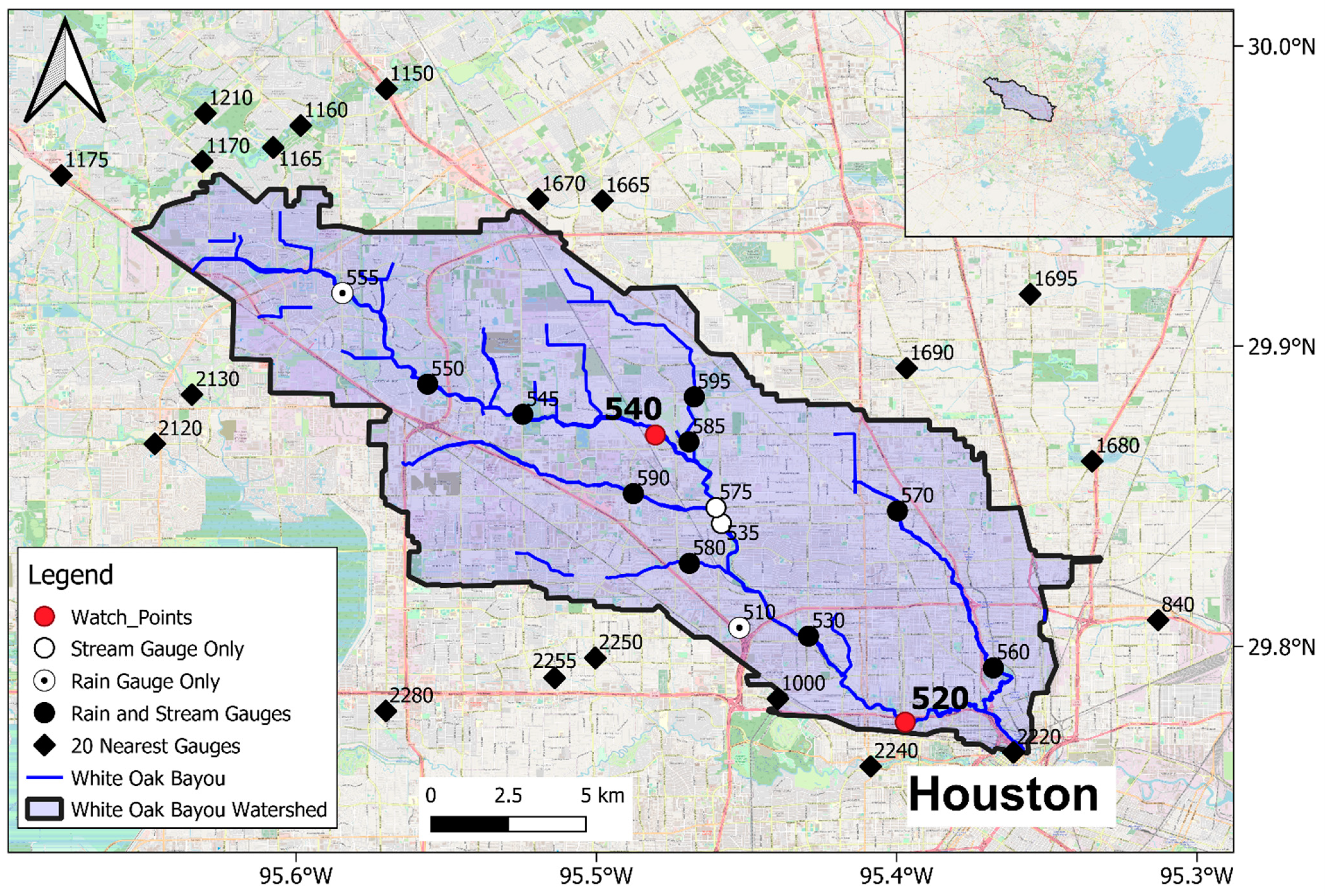
The study area is the White Oak Bayou (WOB) watershed located in central Harris County, Texas, and within the city limits of Houston (Figure 1). WOB originates near the intersection of U.S. Highway 290 and Texas State Highway 6 and flows south-easterly for 40 km until it joins Buffalo Bayou in Houston Downtown as shown in Figure 1 [40]. The watershed covers about 285 square kilometers, serves an estimated population over 430,000 [41].
WOB is one of the most flood-prone areas in the U.S. [42], particularly for the mid- to downstream sections in the major channel (section from Gauge 540 “White Oak Bayou @ Alabonson Road” to Gauge 520 “White Oak Bayou @ Heights Boulevard”, as shown in Figure 1). Many homes and businesses have experienced floods repeatedly, and thousands of structures are at risk from extreme flood events [40]. During Hurricane Harvey (2017), unprecedented flooding occurred along the downstream portion of WOB, where water surface elevations in Downtown Houston are averaged between the 1% (100-year) and 0.2% (500-year) annual exceedance probabilities [43]. An estimate of 7830 houses were flooded during Harvey within the WOB watershed [43].
2.2. Development of XGBoost-Based Flood Alert System
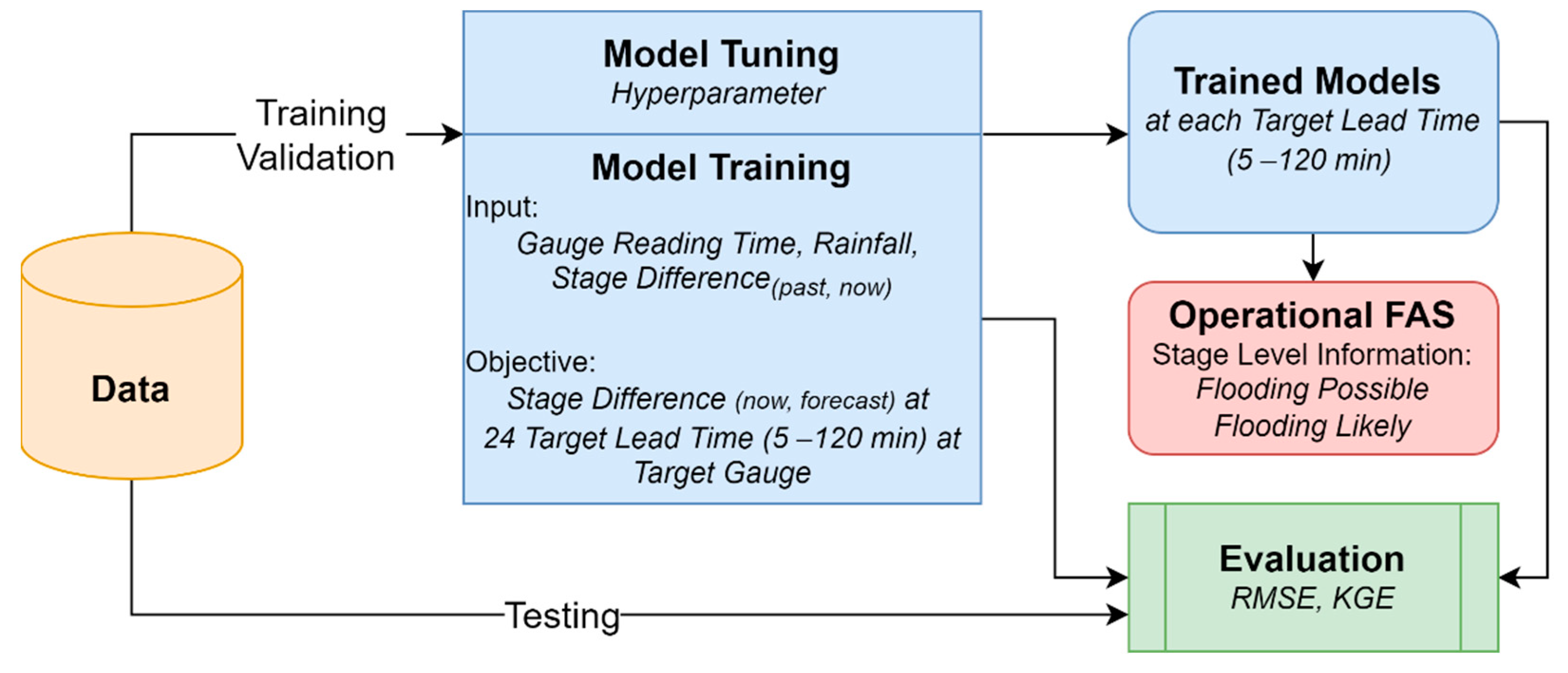
The workflow of the development of XGBoost-based Flood Alert System (FAS) is presented in Figure 2. The details of each workflow component are described in the following sections, including (1) data collection; (2) model development including model tuning and training; (3) operational FAS deployment; and (4) evaluation of the performance. Additionally, the details about the mathematical implementation of the XGBoost algorithm are presented in Supplementary Materials.
2.2.1. Data Collection
In this study, the rainfall and stream level data are retrieved from the gauge networks of the Harris County Flood-Warning System (HCFWS, https://www.harriscountyfws.org/ assessed on 8 January 2021) for the study area (Figure 1). The gauges measure the rainfall (mm) and elevation (m) data at 5-min time interval during the period of January 2010 to December 2019.
The gauge observation data then is allocated into training, validation, and testing datasets for the model development with an objective to minimize the stage difference at watch points. Two watch points (Gauge 520: “White Oak Bayou @ Heights Boulevard” and Gauge 540: “White Oak Bayou @ Alabonson Road”) are selected for this study since both locations are classified as high-risk locations in the watershed (Gauge 520 is the most downstream gauge location in the WOB and Gauge 540 is the gauge location immediate upstream of the confluence section) (Figure 1). The percentages of the training, validation, and testing datasets are carefully determined with a focus to ensure that the training dataset is sufficiently large (70% and 7 years of the total datasets) to capture most of the variability present in the historical period of record (10 years). Table 1 displays information of each dataset, including the percentages, time coverages, and notable historical flood events occurring in the time period of each dataset.
The training dataset provides direct examples of observed inputs and prediction targets for model calibration. Among the training data, two major flood events were included—Memorial Day (2015) and Tax Day (2016). The Memorial Day and the Tax Day storms were both close to a 50-year storm [44]. The validation data (2 years and 3 months) is used to tune XGBoost’s large number of hyperparameters. It is noted that Hurricane Harvey (2017) is included within the validation dataset. Hurricane Harvey (2017) is regarded as one of the most severe tropical cyclones in the United States’ history, according to spatial coverage and peak rainfall amount, during which the entire Harris County received over 70 cm (about 2.3 ft) of rainfall [45]. The extreme nature of the event does not bias model calibration but is still used to evaluate performance in the validation dataset to mimic the impact of a previously unseen extreme event. This leaves 5 months of the testing dataset, which covers two flood events—Flash Flood in May 2019 and Hurricane Imelda in September 2019.
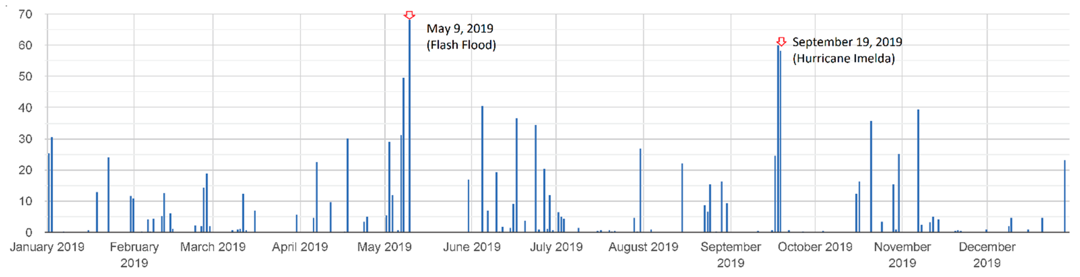
Another objective of this study is to demonstrate and evaluate the performance of real-time XGBoost-based FAS in stage forecasting during major rainfall events. The evaluation metrics are calculated for each watch point under different input configurations (S#1 and S#2). Two major rainfall events occurring at WOB as the test dataset that are targeted by the daily average precipitation time-series analysis in Figure 3. The events occurred on 9 May 2019 (Flash Flood in May) and 19 September 2019 (Hurricane Imelda). Other smaller rainfall events would not be accounted for because they did not cause severe floods.
2.2.2. Performance Evaluation Metrics
Performance of all models is evaluated with Root Mean Squared Error (RMSE) (Equation (1)) and Kling-Gupta Efficiency (KGE) (Equation (2)) [47]. RMSE is used to model the fit of model predictions against observations only in terms of the values of predictions and observations. RMSE is also often used in evaluating the performance of stage forecasting models. Additionally, KGE is a unitless metric that goes incorporating Pearson’s Correlation Coefficient (), the mean of both the observations () and the predictions (), and the standard deviation of both the observations () and the predictions (). KGE = 1 indicates a perfect agreement between simulations and observations
2.2.3. Model Development
In a typical process of machine learning modeling, two types of tunable parameters should be considered: (1) model parameters that are determined during the training phase; and (2) hyperparameters that are set by users before the model training phase (e.g., learning rate, and depth of the tree in XGBoost). In this study, the optimization of hyperparameters is used for balancing the model efficiency and precision which is critical for FAS (Figure 2).
In the model training component, the input variables include the timestamps of the data, rainfall observations, difference between the current and past stage levels, and the output of the learning process is the difference between the current and forecast stages at different lead times (Figure 2). A total of 24 models are trained for the target 24 lead times from 5 to 120 min defined as look-out time windows in 5-min intervals. The models are trained using the same training dataset but with varying hyperparameters. The performance of each model is evaluated with the validation dataset. The differences in model performance are attributed to varied hyperparameters chosen for each model. The best performing models then inform which hyperparameters should be further investigated during the training of additional models. The optimized hyperparameters is established by up to 100 gradient boosted estimators, with a learning rate of 0.1 and maximum tree depth of 4.
One of the objectives of this study is to evaluate if additional hydrologic information is needed to enhance the model performance in terms of both lead time and accuracy, as suggested by a previous study [48]. Therefore, two scenarios are examined in this study: Scenario #1 (S#1) utilizes the 12 rain gauges and 12 stage gauges located within WOB, while Scenario #2 (S#2) includes all gauges used in Scenario #1 with additional 20 rain gauges nearest but outside of the WOB watershed boundary. The rain and stream gauges included in S#1 are illustrated in Figure 1 as “Rain and Stream Gauges” or “Rain Gauges” in round shape while S#2 includes all S#1 gauges in addition to the “20 Nearest Rain Gauges” in diamond shape. This study will also test if the rainfall information in the surrounding areas of the watershed will be applicable to extend the lead times of the FAS.
For each gauge and scenario pair, and for each target lead time (denoted 1–24 when in 5-min intervals), a model is trained for a series of lookback windows (also denoted 1–24 when in 5-min intervals) and then selected a specific lookback window based on validation error (Figure 2). The overall performance of the best model for the target lead time in both scenarios is presented in term of RMSE (Table 2) and KGE (Table 3).
For RMSE, the performance of the models of both Gauges 520 and 540 decreases from 5 min consistently until 120 min of lead time. For KGE, the performance of the models of Gauge 520 increases gradually from 5 min to around 60 min of lead time, then decreases consistently until 120 min of lead time. In contrast, the performance of the models of Gauge 540 decreases consistently from 5 min until 120 min of lead time. There is no significant difference between Scenario #1 and Scenario #2 for both watchpoints indicated by RMSE and KGE metrics. Overall, the XGBoost models demonstrate good performance with the adequacy in potential for further development of FAS.
2.2.4. Flood Alert Design
In this study, a continuous mode of the operating FAS is constructed with an ensemble approach with individual models trained for each lead time. At a given moment in time, the system begins by comparing the current observed stage at the watch point to its critical stages (e.g., flooding likely and flooding possible stage levels, according to HCFWS). The flood-warning decision is made based on the following logics:
- If the current stage exceeds the critical stage, then the system will report flooding;
- If the current stage does not exceed the critical stage, then predictions for all available target lead times will be made using a set of trained models;
- If none of the predicted stages exceeds the critical stage, then all-clear will be reported; and
- If one or more models predict stages exceeding the critical stage, then the smallest target lead time will be reported by the system.
Due to the uncertainties from solely using one model’s output, the ensemble approach is employed to improve the performance of FAS. Based on critical experiments and validation, FAS issues alerts when at least three (3) models forecast stages exceeding the critical stages. The performance of the operational FAS is discussed in the result section in terms of both the accuracy of stage forecasting and the timeliness of the alerts issued by the system.
3. Results
3.1. Model Performance Evaluation
3.1.1. Quantitative Analysis of Model Performance
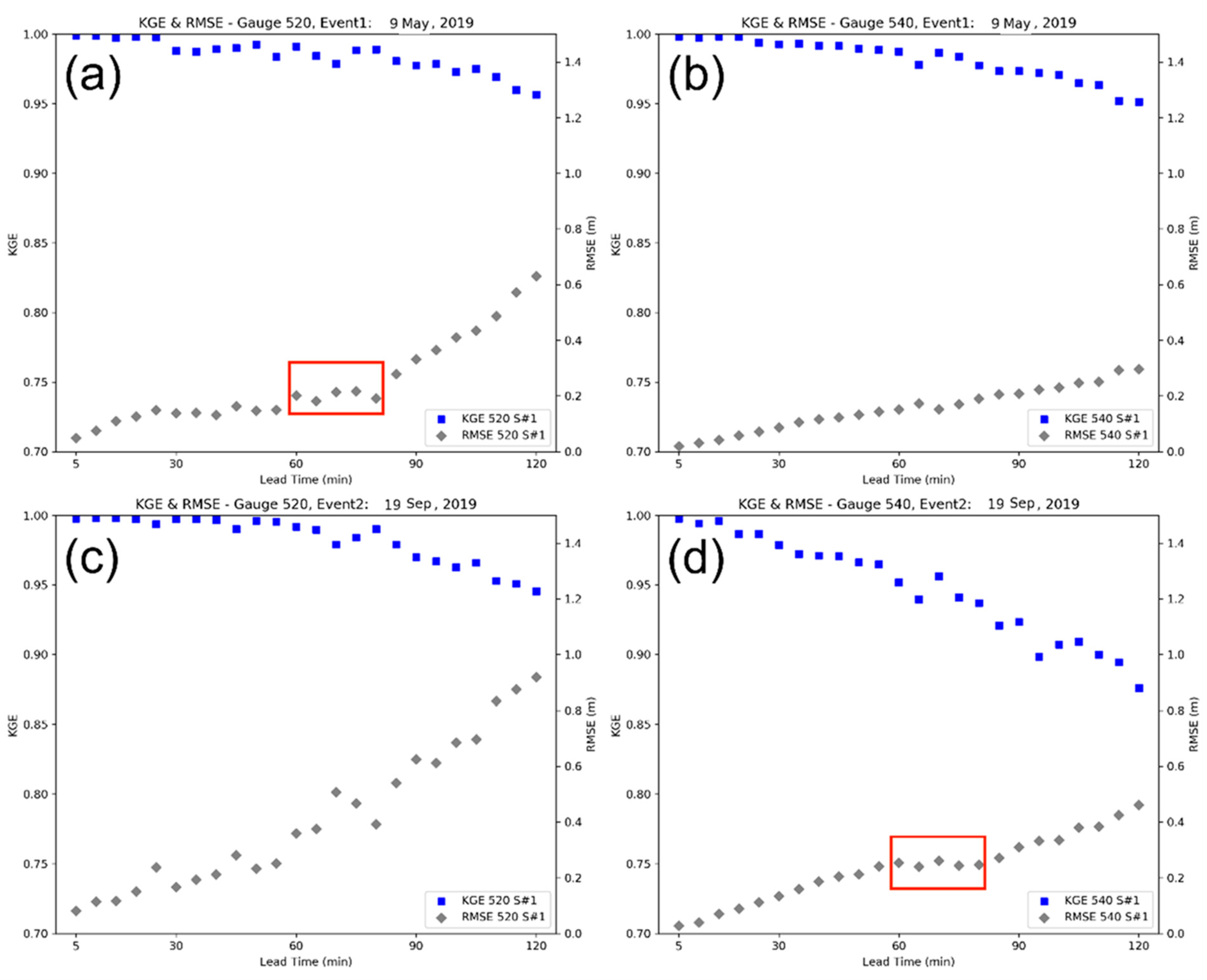
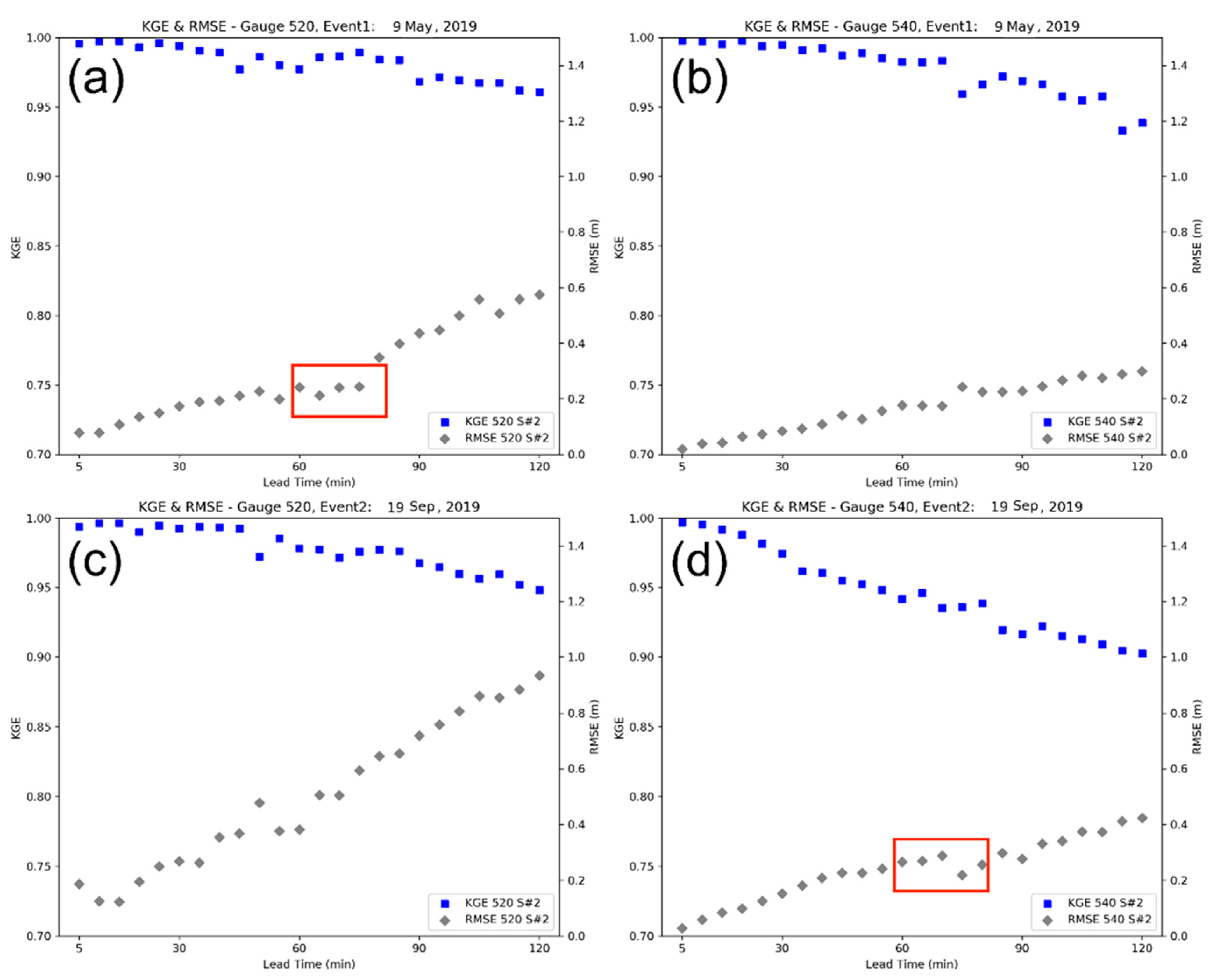
The performance of the FAS in forecasting stages is evaluated by both KGE and RMSE metrics as presented in Figure 4 (S#1) and Figure 5 (S#2) for two major storm events in WOB (9 May 2019 and 19 September 2019). Each model with lead time between 5 min and 2 h (24 models in total) is included in each figure, with the primary axis showing KGE and the secondary axis showing RMSE, for both scenarios.
During the May 2019 event, the S#1 models at Gauge 520 (Figure 4a) show slow increase of RMSE up to 0.2 m with lead times less than 80 min. Then the RMSE values rapidly increase up to 0.6 m at the 120-min lead time. Unlike Gauge 520, the S#1 models at Gauge 540 (Figure 4b) show RMSE values gradually increase up to around 0.3 m at the 120-min lead time. The KGE values decrease along with longer lead times and the lowest value is around 0.95, as presented in both gauges (Figure 4a,b). During the September 2019 event, the S#1 models at Gauge 520 (Figure 4c) show rapid increase of RSME up to around 1 m at the 120-min lead time, while the S#1 models at Gauge 540 (Figure 4d) show RMSE values gradually increase up to around 0.5 m at the 120-min lead time. Unlike the May 2019 event, the September 2019 event shows lower KGE values especially for the models with lead time longer than 60 min in both gauges (Figure 4c,d).
During the May 2019 event, the S#2 models at Gauge 520 (Figure 5a) show gradual increase up to 0.6 m at the 120-min lead time. Unlike Gauge 520, the S#2 models at Gauge 540 (Figure 5b) show RMSE values gradually increase up to around 0.3 m at the 120-min lead time, which is similar to what is shown in Figure 4b. The KGE values at Gauge 540 show generally lower values than those at Gauge 520 (Figure 5a), with lowest value around 0.93 at the 115-min lead time (Figure 5b). During the September 2019 event, the S#2 models at Gauge 520 (Figure 5c) also show rapid increase of RSME up to around 1 m at the 120-min lead time, which is comparable to what is shown in Figure 4c. Similar to what is presented in Figure 4d, the S#2 models at Gauge 540 (Figure 5d) show RMSE values gradually increase up to above 0.4 m at the 120-min lead time. In addition, there is generally no significant pattern difference between the S#1 (Figure 4c,d) and S#2 (Figure 5c,d) models in terms of KGE values in September 2019 event, while the S#2 models show slightly higher KGE values than the S#1 models at Gauge 540 (Figure 5d). It is noted that both scenarios have a consistent performance within 60–80 min lead-time models evaluated by RMSE, as shown in the red boxes in Figure 4a,d and Figure 5a,d.
Above all, the S#1 models show a slightly better performance than the S#2 models during the May 2019 event at Gauge 520 (Figure 4a and Figure 5a), while the S#2 models show a marginally better performance than that the S#1 models during the September 2019 event at Gauge 540 (Figure 4d and Figure 5d). Both models have similar performances in other cases (Figure 4b,c and Figure 5b,c), suggesting that the models using external gauge information (S#2) yield similar performance with the models without (S#1) evaluated by both KGE and RMSE metrics.
3.1.2. Comparison of Measured and Forecasted Stages
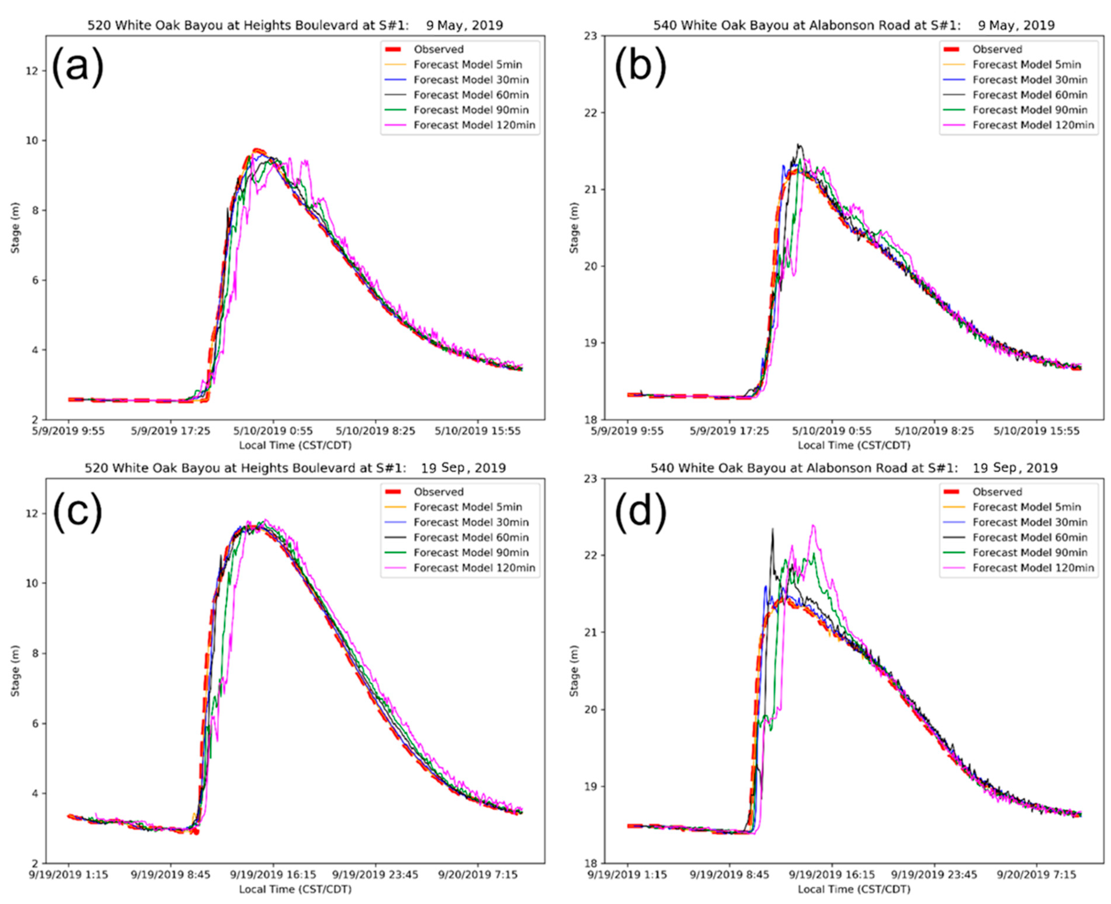
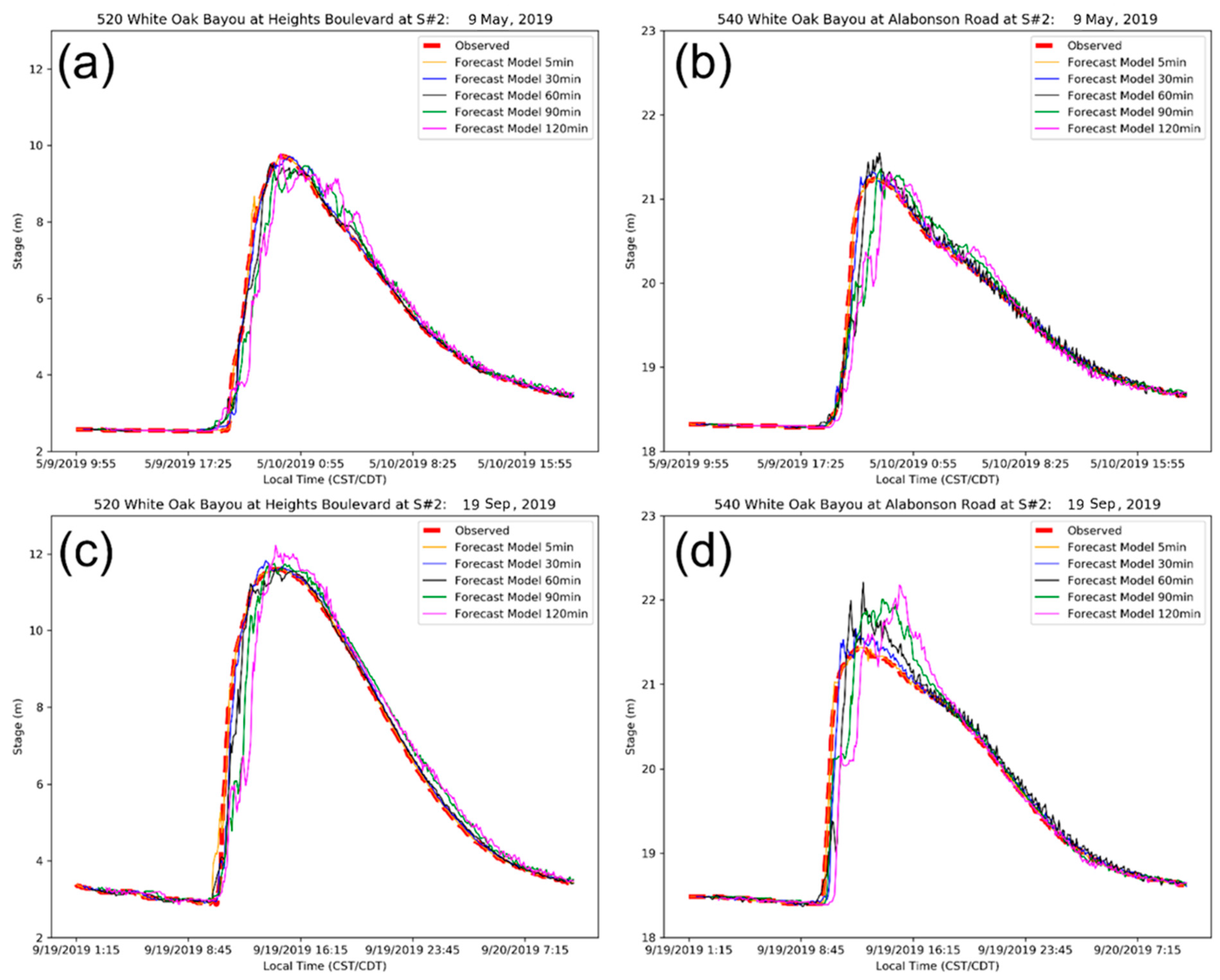
Furthermore, model performance in predicting the rising and falling limbs of the stages is also evaluated by comparing predicted stage hydrographs against observed stage hydrographs in Figure 6 (S#1) and Figure 7 (S#2). The red dotted lines represent observed stage hydrographs and other lines represent the predicted stage hydrographs in 5 min, 30 min, 60 min, 90 min, and 120 min models (colored as yellow, blue, black, green, and magenta, respectively). To a certain extent, each model’s forecast fits the shape of the observed stage. The predicted stage hydrographs from the 5-min and 30-min lead-time models match the observations admirably, indicating a good performance of XGBoost-based FAS in shorter lead time forecasts. However, the 60-min lead-time models still reach a good amount of agreement in both the stage and peak timing. Beyond 60 min, the lead-time models tend to underestimate the rising limbs and overestimate the falling limbs for both Gauge 520 and 540 locations. It is also noted that the longer lead-time models (e.g., 120-min lead-time model) tend to delay the prediction of the rising and falling of the stages in comparison to the observed stages.
Comparing the system performance between different scenarios, one should note that in S#1 (Figure 6a,c) the predictions fit the observation curves better than those in S#2 (Figure 7a,c) at Gauge 520. At Gauge 540, both results tend to overestimate the peak stages (Figure 6d and Figure 7d), where the overestimation that is found in the S#2 models is less than that of the S#1 models.
3.2. Evaluation of Real-Time Stage Forecasting
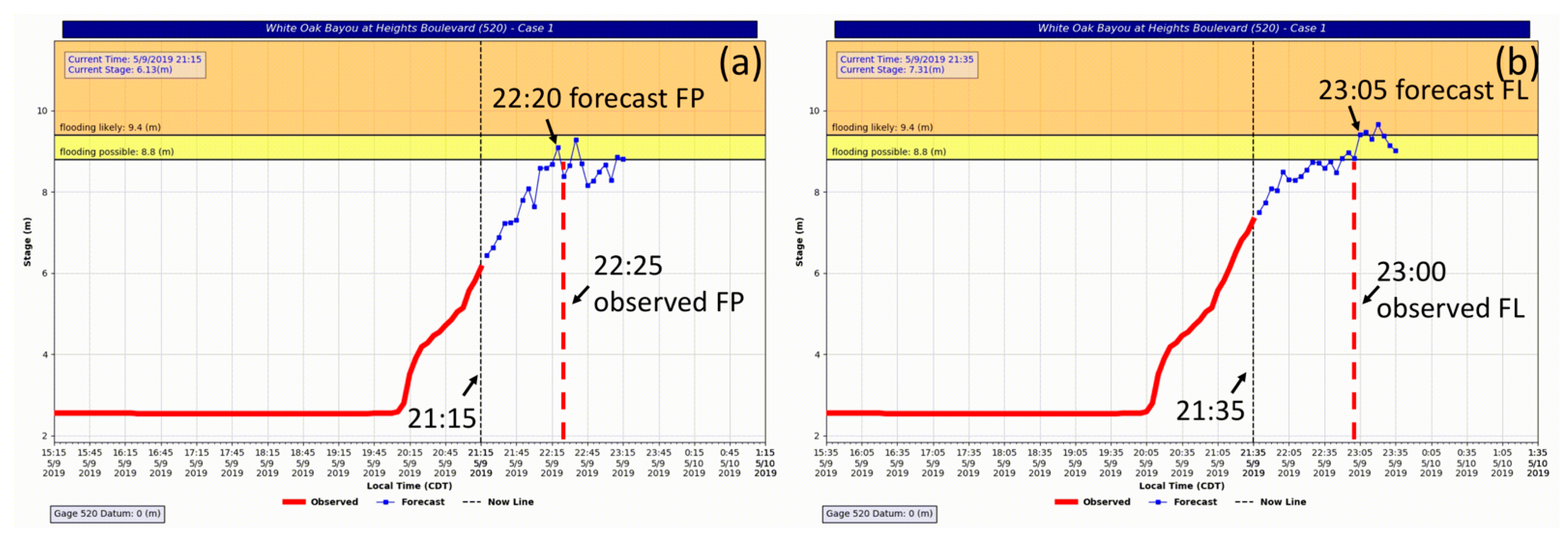
In the essence of evaluating flood-warning systems, assessment has been focused on predicting the timing of the rising limb of an event so the emergency responders can have time to act before flood occurs. In addition, accurate prediction of the critical stage levels that are closely linked with the severity of floods is also required. Hence, the XGBoost-based FAS is evaluated during the rising limbs for both events (May and September 2019) with respect to both scenarios (S#1 and S#2) at Gauges 520 and 540 as shown in Figure 8, Figure 9, Figure 10, Figure 11, Figure 12 and Figure 13 and each figure represents a specific case. In Figure 8, Figure 9, Figure 10, Figure 11, Figure 12 and Figure 13, forecasts (blue lines) are made to the right of the now lines (vertical dotted lines) corresponding to each target lead-time model (blue dots). Left of the now lines is to show observed stages (red lines). As described in Section 2.2.4, the system issues either flooding possible (FP) or flooding likely (FL) warning when at least three (3) forecasted stages are higher than the critical stages of FP or FL, respectively. Visually, it means at least three blue dots enter into the yellow (FP) or orange (FL) area to trigger the warning. Both FP and FL stages are determined and provided by the local authority (e.g., https://www.harriscountyfws.org/GageDetail/Index/520?From=1/6/2022%204:23%20PM&span=2%20Days&r=1&v=surfaceBox&selIdx=0 assessed on 8 January 2021), where FL stage is typically the road/bridge deck elevation and FP stage is slightly lower than FL stage. The observed critical stages of either FP, FL, or peak stage (PS) that are notified by the red vertical dotted lines with the times when the certain stages are observed. The information of Figure 8, Figure 9, Figure 10, Figure 11, Figure 12 and Figure 13 is summarized into Table 4, where the “Forecasted Lead Time” indicates the differences between the current time and predicted time of critical stages and the “Observed Lead Time” indicates the differences between the current time and observed time of critical stages. The differences between these two types of lead time are calculated and summarized in the “Difference of Lead Times (Forecasted—Observed)”.
Starting with Gauge 520 in S#1, at 9 May 2019 21:15 during the May 2019 event, the models for S#1 issue the FP warning with the forecasted lead time of 65 min (Figure 8a, Table 4), which is 5 min ahead of the observed FP stage (22:25). For the same event, the S#1 models issue the FL warning at 9 May 2019 21:35 with the forecasted lead time of 90 min (Figure 8b, Table 4), which is 5 min later than the observed FL stage (23:00).
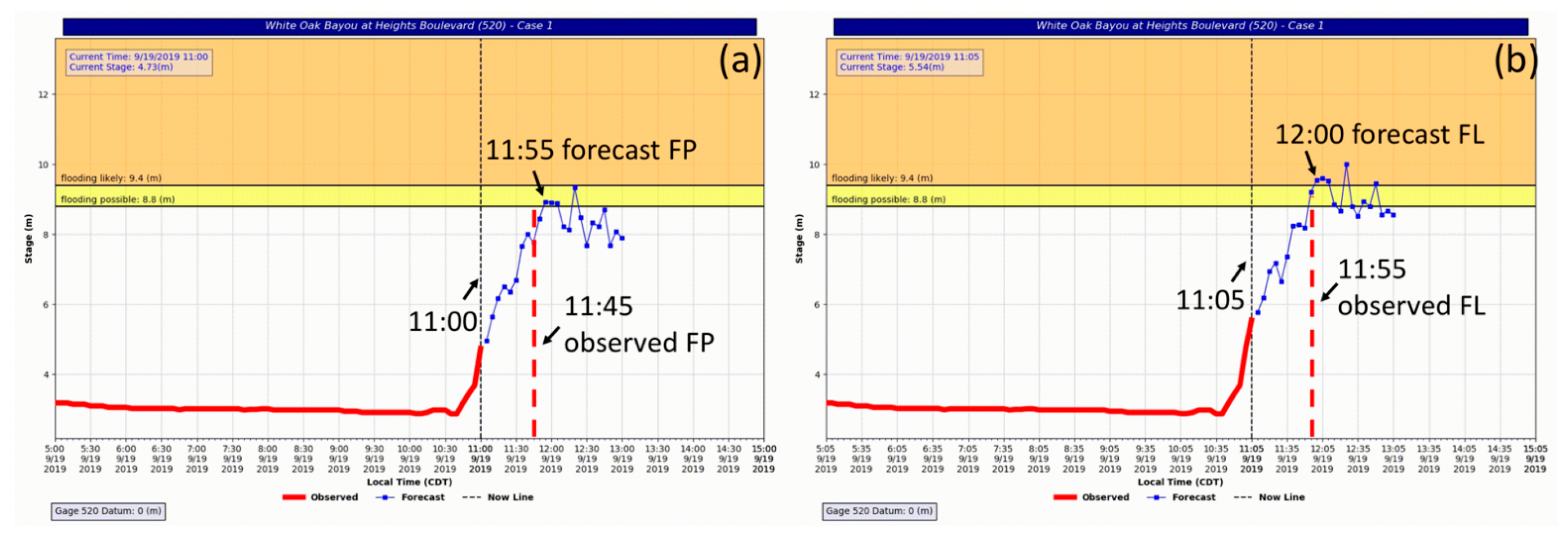
At 19 September 2019 11:00 during the September 2019 event, the S#1 models issue the FP warning at Gauge 520 with the forecasted lead time of 55 min (Figure 9a, Table 4), which is 10 min later than the observed FP stage (11:45). For the same event, the S#1 models issue the FL warning at 19 September 2019 11:05 with the forecasted lead time of 55 min (Figure 9b, Table 4), which is 5 min later than the observed FL stage (23:00).
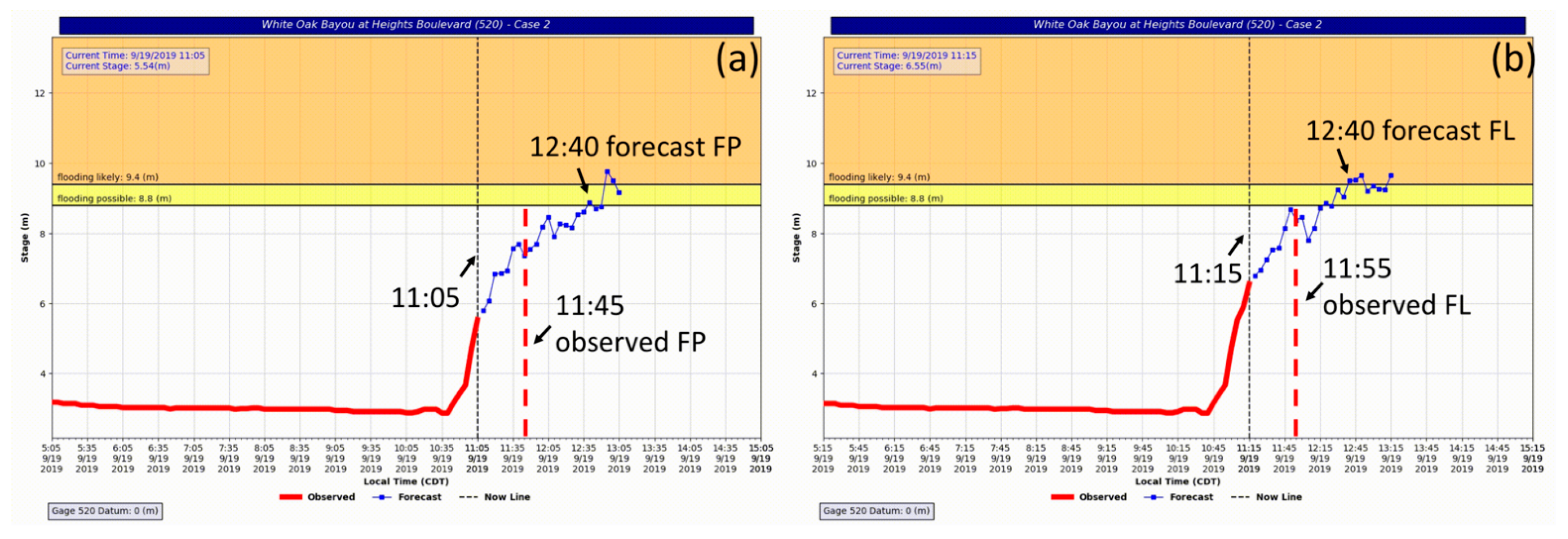
Continuing with Gauge 520 in S#2, at 9 May 2019 21:15 during the May 2019 event, the S#2 models issue the FP warning with the forecasted lead time of 110 min (Figure 10a, Table 4), which is 40 min later than the observed FP stage (22:25). For the same event, the S#2 models issue the FL warning at 9 May 2019 21:30 with the forecasted lead time of 110 min (Figure 10b, Table 4), which is 20 min later than the observed FL stage (23:00).
At 19 September 2019 11:05 during the September 2019 event, the S#2 models issue the FP warning at Gauge 520 with the forecasted lead time of 95 min (Figure 11a, Table 4), which is 55 min later than the observed FP stage (11:45). For the same event, the S#2 models issue the FL warning at 19 September 2019 11:15 with the forecasted lead time of 85 min (Figure 11b, Table 4), which is 45 min later than the observed FL stage (23:00).
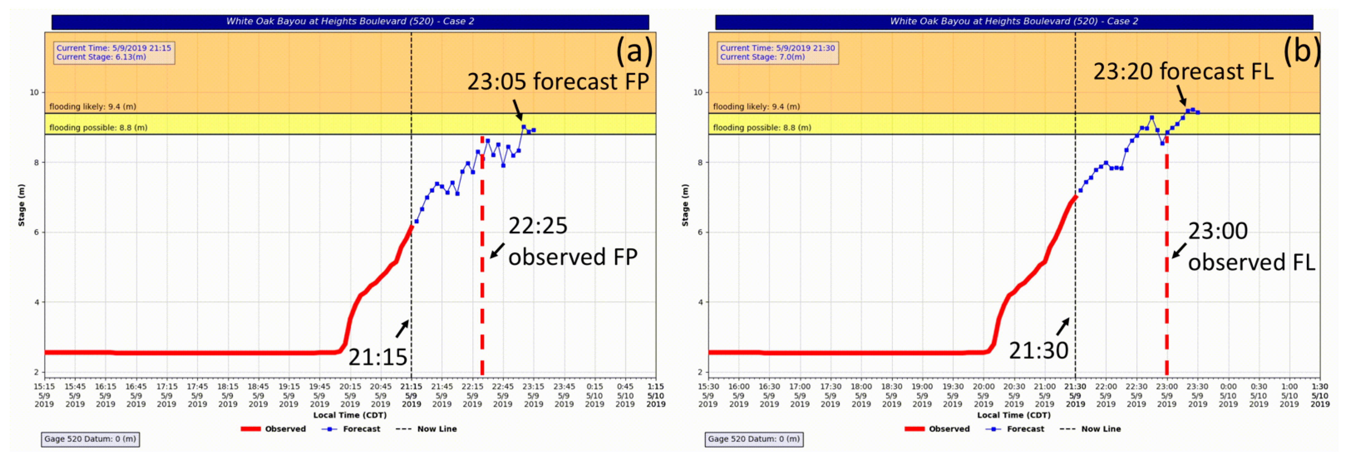
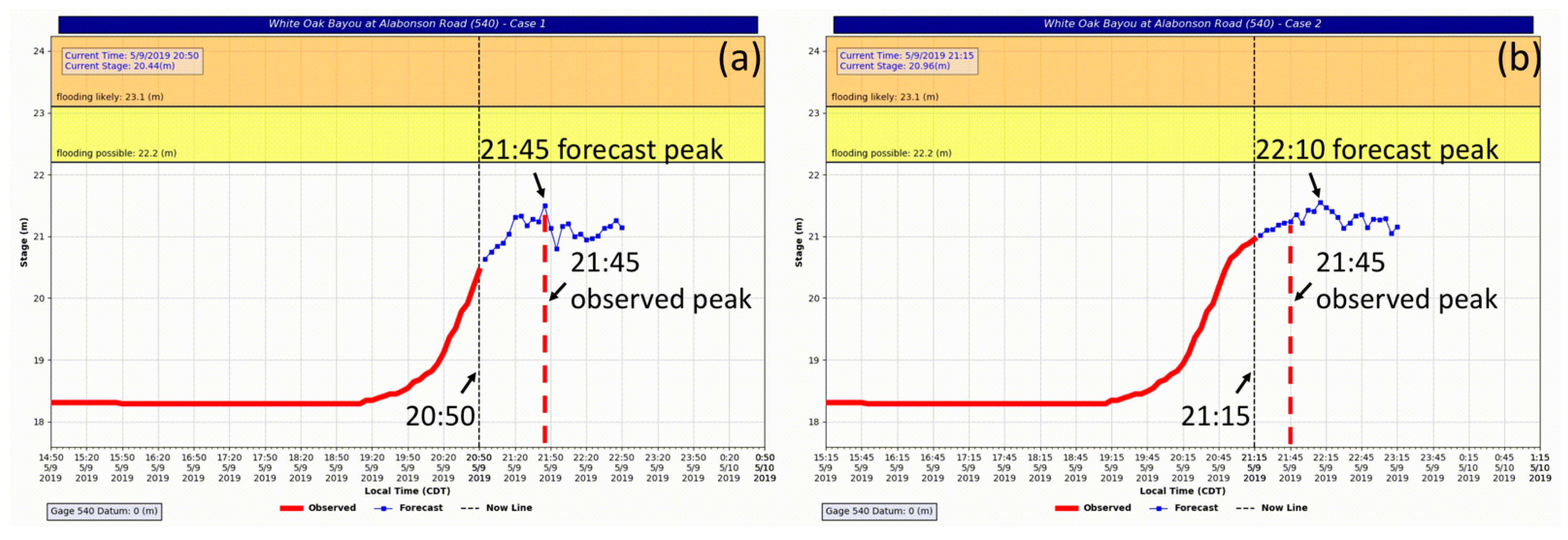
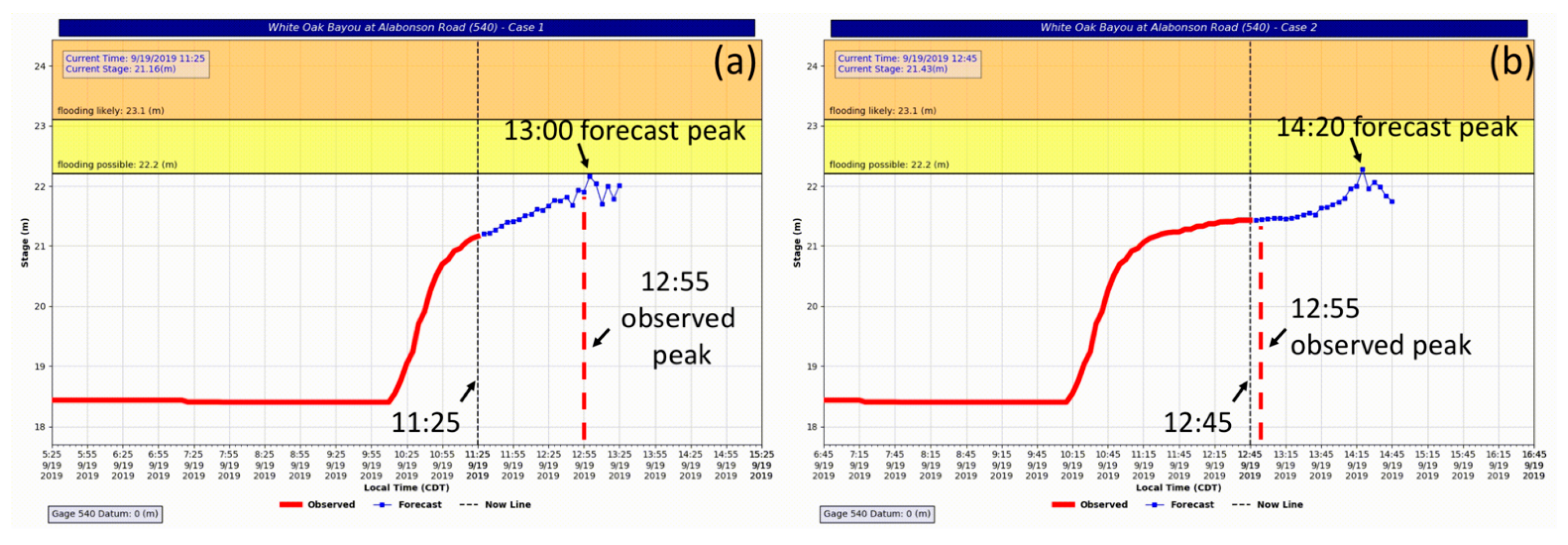
At Gauge 540, the stages do not reach the FP or FL stages during the testing time-period, thus the models are evaluated based on the peak stage forecasting during the events for both scenarios. For the May 2019 event, the S#1 models precisely predict the arrival time of the peak stage (09 May 2019 21:45) with lead time of 55 min (Figure 12, Table 4). Comparably, the S#2 models predict the peak stage 25 min later than the observed peak stage (Figure 12b, Table 4). For the September 2019 event, the S#1 models also achieve accurate forecasted peak stage 5 min later than the observed peak stage (Figure 13a, Table 4), while the forecasts of S#2 models significantly delay the arrival time of peak stage, which is 85 min later than the observed peak stage (Figure 13b and Table 4).
4. Discussion
In this study, a flood alert system (FAS) based on individual XGBoost models has demonstrated a good usability for running in a continuous mode. Unlike other event-based FAS, the XGBoost-based FAS does not require an external starting trigger to switch on. It can constantly run in the backend, detect an impending event according to pre-determined critical stages, and automatically generate notifications to first-responders in real time.
Besides its unique feature of continuous operations, the XGBoost-based FAS demonstrates good performance in predicting stages according to the evaluation criteria of: RMSE and KGE metrics; forecast of rising limbs, and prediction of the timings of critical stages.
Firstly, the XGBoost-based FAS is evaluated by RMSE and KGE metrics. The results in Table 2 and Table 3 show superior performance by both metrics for the model validation. The results in Figure 4 and Figure 5 further demonstrate sufficient performance for both the May and September 2019 events during the model-testing phase. Compared with RMSE, KGE serves as a more favorable criterion that has been commonly applied and suggested for evaluating the performance of hydrologic models for its less sensitivity to the high values [47]. Comparing the KGE values of the models, one can see better performance to be achieved at Gauge 520 (Figure 4a,c and Figure 5a,c) than Gauge 540 (Figure 4b,d and Figure 5b,d) while the RMSE values at Gauge 520 are found generally higher than Gauge 540 in this study.
Secondly, the forecast of rising limbs of stage hydrographs is critical for evaluating the performance of FAS. While rising limbs are relatively challenging to predict due to the uncertainties in rainfall intensity and location, initial soil moisture conditions, etc., the rising limbs of predicted stage hydrographs from the XGBoost-based FAS certainly demonstrate a satisfactory consistency with the observed stages in terms of timings and shapes (Figure 6 and Figure 7). This is very important for emergency personnel to initiate prompt flood mitigation measures during real-time operations.
Lastly, the accuracy in predicting of the occurring times of critical stages (flooding possible, flooding likely, and peak stage) is also a key element in evaluating FAS performance. Figure 8a,b Figure 9a,b, Figure 12a and Figure 13a show that the S#1 models can achieve good performance in forecasting the timings of critical stages (no more than 10 min difference as shown in “Difference of Lead Times” in Table 4) with longer lead times (55–95 min) (Table 4). It is noted that some of the S#1 models have 5–10 min delay in predicting the times of the critical stages mainly due to the mechanism of how the system triggers the flood possible (FP) and flood likely (FL) alerts only when at least three models predict the stage levels are over the FP or FL levels. It is a conservative engineering approach that will likely result in a short delay as shown in Table 4. From a flood-warning system/application standpoint, we believe that this conservative engineering design can reduce unnecessary overreactions and the delay of less than 10 min is acceptable in flood practices, considering that system interval is at a 5-min step based on the temporal resolution of the source data. The delay times can be reduced by utilizing finer temporal resolution (e.g., 1-min) data, as well as implementing a more aggressive alerting design (e.g., triggering flood alert whenever one of the models firstly predicts higher values than the critical stages). On-going research will be reported in a forthcoming paper for this particular effort.
While Young and others [48] suggested additional hydrologic information (e.g., additional input from HEC-HMS predictions) for improving the model performance, this study counterintuitively shows the models using more gauge information (S#2) lead to diminished performance compared with S#1 models (Table 4) and that KGE and RMSE metrics remain relatively similar for both scenarios (Figure 4 and Figure 5). The authors think that there could be several reasons: firstly, using more information of the watershed might have weakened the overall performance as shown in S#2 (S#2 includes additional rain gauges from outside the watershed in addition to the same information with which the S#1 is configured). It is noted that stage data from the stream gauges as used in the S#1 serves as more direct information for stage forecasting than the information obtained from the rain gauges. Secondly, it is also likely that the major storms recorded by the gauges outside the watershed have a negative impact on the stage prediction through less accurate and indirect information. Lastly, the XGBoost models utilize all the input variables directly without preprocessing or selection and a proper selection of input variables is needed to improve the performance of the XGBoost models [49]. Overall, the results of this study suggest that including the gauge information only from the inside of the watershed as configured in S#1 is adequate and advantageous for training XGBoost models for flood-warning practices. Instead, the internal spatial information of the watershed, such as variables of physical conditions (e.g., soil moisture, land cover, land use, etc.), as well as other available geological, geomorphological, and hazard data can be more applicable when they are integrated into the flood-alert system to improve its performance in flood-critical areas for civil-protection purposes [50].
5. Conclusions
The performance of flood-alert systems (FAS) directly depends on the accuracy and timings of the forecasted stages. Because of the limitations of physics-based hydrometeorological models in representing complex meteorological and hydrologic processes, data-driven models as an alternative approach have become increasingly necessary to improve the performance of FAS.
In this study, the XGBoost-based FAS is developed and evaluated, which runs in a continuous mode and automatically detects flood events by forecasting stage information from 5 min up to 2 h in a 5-min temporal interval. Quantitative evaluations of the models show good performance indicated by RMSE and KGE metrics and the shapes of the predicted stage hydrographs match well with the observed stage hydrographs. Moreover, XGBoost-based models are tested with Scenario #1 (utilizing the gauge data within the study area only) and Scenario #2 (having additional gauge data outside the study area). The results from the comparative analysis suggest that while both scenarios achieve similar performance, as indicated by KGE and RMSE metrics, the additional information from the gauges outside of the watershed as configured in Scenario #2 has a negative impact on predicting the critical stages.
While the XGBoost-based FAS achieves satisfactory performance with showing promising future for operational deployment, the authors believe that the performance of the system can be further improved in the following perspectives:
- Improving the design of the FAS warning criteria: the current system issues alerts when at least three (3) target lead-time models predict all stage values over a critical level. Although the criteria have been proved to be effective based on the experiments and engineering judgement, this design is still regarded as an empirical approach and will need to be further investigated with more analyses.
- Considering the rainfall characteristics of flood events: the types of the rainfall are not currently classified in the testing and validation datasets for the FAS (e.g., the May 2019 event was produced by a cold front and the 19 September event was caused by a tropical cyclone—Hurricane Imelda). Different types of rainfall may have distinct impacts on the FAS performance due to their spatiotemporal characteristics that are indirectly reflected in the gauge readings (Table 4). An on-going study on this topic will be reported in a forthcoming paper.
- Introducing spatial information relative to the watershed: the XGBoost-based FAS is built solely based on the temporal scale without incorporating any level of spatial information. Gauge readings are fed to the models as independent inputs without any spatial weighting as performed. The authors think that the spatial information representing the physical conditions of the watershed (e.g., initial soil moisture, watershed size, land use, etc.) need to be factored in the training process to further enhance the prediction performance.
Supplementary Materials
The following are available online at https://www.mdpi.com/article/10.3390/w14050747/s1, Introduction to XGBoost Algorithm.
Author Contributions
Conceptualization, Z.N.F., W.S. and D.L.; methodology, W.S. and D.L.; software, W.S.; validation, W.S., D.L. and W.L.; formal analysis, W.S., D.L. and Z.N.F.; investigation, Z.N.F., W.S. and D.L.; resources, N.F and D.L.; data curation, W.S.; writing—original draft preparation, W.S. and D.L.; writing—review and editing, W.L., D.L. and W.L.; visualization, W.S., D.L. and W.L.; supervision, Z.N.F.; project administration, Z.N.F. and D.L.; funding acquisition, Z.N.F. All authors have read and agreed to the published version of the manuscript.
Funding
This research received no external funding.
Institutional Review Board Statement
Not applicable.
Informed Consent Statement
Not applicable.
Data Availability Statement
Not applicable.
Acknowledgments
The authors would like to thank the data supported from Harris County Flood-Warning System.
Conflicts of Interest
The authors declare no conflict of interest.
References
- Mosavi, A.; Ozturk, P.; Chau, K. Flood Prediction Using Machine Learning Models: Literature Review. Water 2018, 10, 1536. [Google Scholar] [CrossRef] [Green Version]
- Smith, A.B. U.S. Billion-Dollar Weather and Climate Disasters, 1980–Present (NCEI Accession 0209268); National Centers for Environmental Information: Asheville, NC, USA, 2020.
- Fang, Z.; Dolan, G.; Sebastian, A.; Bedient, P.B. Case Study of Flood Mitigation and Hazard Management at the Texas Medical Center in the Wake of Tropical Storm Allison in 2001. Nat. Hazards Rev. 2014, 15, 05014001. [Google Scholar] [CrossRef]
- Fares, A. Climate Change and Extreme Events; Elsevier: San Diego, CA, USA, 2021; ISBN 978-0-12-823288-0. [Google Scholar]
- United Nations Economic and Social Commission for Asia and the Pacific (ESCAP) Flood Forecasting and Early Warning in Transboundary River Basins: A Toolkit. Available online: https://www.unescap.org/resources/flood-forecasting-and-early-warning-transboundary-river-basins-toolkit (accessed on 9 March 2021).
- Pappenberger, F.; Cloke, H.L.; Parker, D.J.; Wetterhall, F.; Richardson, D.S.; Thielen, J. The Monetary Benefit of Early Flood Warnings in Europe. Environ. Sci. Policy 2015, 51, 278–291. [Google Scholar] [CrossRef]
- Eslamian, S. (Ed.) Handbook of Engineering Hydrology. Fundamentals and Applications; CRC Press, Taylor & Francis Group: Boca Raton, FL, USA, 2013; ISBN 978-1-4665-5241-8. [Google Scholar]
- Hussain, F.; Wu, R.-S.; Wang, J.-X. Comparative Study of Very Short-Term Flood Forecasting Using Physics-Based Numerical Model and Data-Driven Prediction Model. Nat. Hazards 2021, 107, 249–284. [Google Scholar] [CrossRef]
- Christian, J.; Fang, Z.; Torres, J.; Deitz, R.; Bedient, P. Modeling the Hydraulic Effectiveness of a Proposed Storm Surge Barrier System for the Houston Ship Channel during Hurricane Events. Nat. Hazards Rev. 2015, 16, 04014015. [Google Scholar] [CrossRef]
- Torres, J.M.; Bass, B.; Irza, N.; Fang, Z.; Proft, J.; Dawson, C.; Kiani, M.; Bedient, P. Characterizing the Hydraulic Interactions of Hurricane Storm Surge and Rainfall–Runoff for the Houston–Galveston Region. Coast. Eng. 2015, 106, 7–19. [Google Scholar] [CrossRef] [Green Version]
- Fang, Z.N.; Shultz, M.J.; Wienhold, K.J.; Zhang, J.; Gao, S. Case Study: Comparative Analysis of Hydrologic Simulations with Areal-Averaging of Moving Rainfall. Hydrology 2019, 6, 12. [Google Scholar] [CrossRef] [Green Version]
- Zhang, J.; Lin, P.; Gao, S.; Fang, Z. Understanding the Re-Infiltration Process to Simulating Streamflow in North Central Texas Using the WRF-Hydro Modeling System. J. Hydrol. 2020, 587, 124902. [Google Scholar] [CrossRef]
- Najibi, N.; Devineni, N.; Lu, M.; Perdigão, R.A.P. Coupled Flow Accumulation and Atmospheric Blocking Govern Flood Duration. Npj Clim. Atmos. Sci. 2019, 2, 19. [Google Scholar] [CrossRef]
- Franchini, M.; Lamberti, P. A Flood Routing Muskingum Type Simulation and Forecasting Model Based on Level Data Alone. Water Resour. Res. 1994, 30, 2183–2196. [Google Scholar] [CrossRef]
- Krzysztofowicz, R.; Herr, H.D. Hydrologic Uncertainty Processor for Probabilistic River Stage Forecasting: Precipitation-Dependent Model. J. Hydrol. 2001, 249, 46–68. [Google Scholar] [CrossRef]
- Krzysztofowicz, R. Bayesian System for Probabilistic River Stage Forecasting. J. Hydrol. 2002, 268, 16–40. [Google Scholar] [CrossRef]
- Krzysztofowicz, R. Bayesian Theory of Probabilistic Forecasting via Deterministic Hydrologic Model. Water Resour. Res. 1999, 35, 2739–2750. [Google Scholar] [CrossRef] [Green Version]
- Fang, Z.; Bedient, P.B.; Buzcu-Guven, B. Long-Term Performance of a Flood Alert System and Upgrade to FAS3: A Houston, Texas, Case Study. J. Hydrol. Eng. 2011, 16, 818–828. [Google Scholar] [CrossRef]
- Vieux, B.E.; Cui, Z.; Gaur, A. Evaluation of a Physics-Based Distributed Hydrologic Model for Flood Forecasting. J. Hydrol. 2004, 298, 155–177. [Google Scholar] [CrossRef]
- Symonds, A.M.; Vijverberg, T.; Post, S.; Van der Spek, B.-J.; Henrotte, J.; Sokolewicz, M. Comparison between MIKE 21 FM, Delft3D and Delft3D FM Flow Models of Western Port Bay, Australia. Int. Conf. Coastal. Eng. 2017, 11. [Google Scholar] [CrossRef]
- Bates, P.D.; De Roo, A.P.J. A Simple Raster-Based Model for Flood Inundation Simulation. J. Hydrol. 2000, 236, 54–77. [Google Scholar] [CrossRef]
- Collier, C.G. Flash Flood Forecasting: What Are the Limits of Predictability? Q. J. R. Meteorol. Soc. 2007, 133, 3–23. [Google Scholar] [CrossRef]
- Nayak, P.C.; Sudheer, K.P.; Rangan, D.M.; Ramasastri, K.S. Short-Term Flood Forecasting with a Neurofuzzy Model: Flood Forecasting with a Neurofuzzy Model. Water Resour. Res. 2005, 41. [Google Scholar] [CrossRef] [Green Version]
- Hosseiny, H.; Nazari, F.; Smith, V.; Nataraj, C. A Framework for Modeling Flood Depth Using a Hybrid of Hydraulics and Machine Learning. Sci. Rep. 2020, 10, 8222. [Google Scholar] [CrossRef]
- Tu, H.; Wang, X.; Zhang, W.; Peng, H.; Ke, Q.; Chen, X. Flash Flood Early Warning Coupled with Hydrological Simulation and the Rising Rate of the Flood Stage in a Mountainous Small Watershed in Sichuan Province, China. Water 2020, 12, 255. [Google Scholar] [CrossRef] [Green Version]
- Shen, C.; Laloy, E.; Elshorbagy, A.; Albert, A.; Bales, J.; Chang, F.-J.; Ganguly, S.; Hsu, K.-L.; Kifer, D.; Fang, Z.; et al. HESS Opinions: Incubating Deep-Learning-Powered Hydrologic Science Advances as a Community. Hydrol. Earth Syst. Sci. 2018, 22, 5639–5656. [Google Scholar] [CrossRef] [Green Version]
- Meresa, H. Modelling of River Flow in Ungauged Catchment Using Remote Sensing Data: Application of the Empirical (SCS-CN), Artificial Neural Network (ANN) and Hydrological Model (HEC-HMS). Model. Earth Syst. Environ. 2019, 5, 257–273. [Google Scholar] [CrossRef]
- Hwang, S.H.; Ham, D.H.; Kim, J.H. Forecasting Performance of LS-SVM for Nonlinear Hydrological Time Series. KSCE J. Civ. Eng. 2012, 16, 870–882. [Google Scholar] [CrossRef]
- Chang, L.-C.; Shen, H.-Y.; Wang, Y.-F.; Huang, J.-Y.; Lin, Y.-T. Clustering-Based Hybrid Inundation Model for Forecasting Flood Inundation Depths. J. Hydrol. 2010, 385, 257–268. [Google Scholar] [CrossRef]
- Bermúdez, M.; Ntegeka, V.; Wolfs, V.; Willems, P. Development and Comparison of Two Fast Surrogate Models for Urban Pluvial Flood Simulations. Water Resour. Manag. 2018, 32, 2801–2815. [Google Scholar] [CrossRef]
- Liu, Y.; Pender, G. A Flood Inundation Modelling Using V-Support Vector Machine Regression Model. Eng. Appl. Artif. Intell. 2015, 46, 223–231. [Google Scholar] [CrossRef]
- Yaseen, Z.M.; El-shafie, A.; Jaafar, O.; Afan, H.A.; Sayl, K.N. Artificial Intelligence Based Models for Stream-Flow Forecasting: 2000–2015. J. Hydrol. 2015, 530, 829–844. [Google Scholar] [CrossRef]
- Zhang, H.; Yang, Q.; Shao, J.; Wang, G. Dynamic Streamflow Simulation via Online Gradient-Boosted Regression Tree. J. Hydrol. Eng. 2019, 24, 04019041. [Google Scholar] [CrossRef]
- Chen, T.; Guestrin, C. Xgboost: A Scalable Tree Boosting System. In Proceedings of the 22nd ACM SIGKDD International Conference on Knowledge Discovery and Data Mining, San Francisco, CA, USA, 13–17 August 2016; pp. 785–794. [Google Scholar]
- Ma, M.; Zhao, G.; He, B.; Li, Q.; Dong, H.; Wang, S.; Wang, Z. XGBoost-Based Method for Flash Flood Risk Assessment. J. Hydrol. 2021, 598, 126382. [Google Scholar] [CrossRef]
- Abedi, R.; Costache, R.; Shafizadeh-Moghadam, H.; Pham, Q.B. Flash-Flood Susceptibility Mapping Based on XGBoost, Random Forest and Boosted Regression Trees. Geocarto Int. 2021, 1–18. [Google Scholar] [CrossRef]
- Potdar, A.S.; Kirstetter, P.-E.; Woods, D.; Saharia, M. Toward Predicting Flood Event Peak Discharge in Ungauged Basins by Learning Universal Hydrological Behaviors with Machine Learning. J. Hydrometeorol. 2021, 22, 2971–2982. [Google Scholar]
- Guo, W.-D.; Chen, W.-B.; Yeh, S.-H.; Chang, C.-H.; Chen, H. Prediction of River Stage Using Multistep-Ahead Machine Learning Techniques for a Tidal River of Taiwan. Water 2021, 13, 920. [Google Scholar] [CrossRef]
- Nguyen, D.H.; Le, X.H.; Heo, J.-Y.; Bae, D.-H. Development of an Extreme Gradient Boosting Model Integrated With Evolutionary Algorithms for Hourly Water Level Prediction. IEEE Access 2021, 9, 125853–125867. [Google Scholar] [CrossRef]
- White Oak Bayou: An Evolving Urban Waterway; Harris County Flood Control District: Houston, TX, USA, 2000; Retrieved 27 March 2021.
- White Oak Bayou Watershed; Harris County Flood Control District: Houston, TX, USA, July 2013; Retrieved 27 March 2021.
- The Growing Threat of Urban Flooding | Center for Disaster Resilience. Available online: https://cdr.umd.edu/urban-flooding-report (accessed on 2 April 2021).
- Memorandum of Hurricane Harvey; Harris County Flood Control District: Houston, TX, USA, 4 June 2018; Retrieved 27 March 2021.
- Gao, S.; Fang, Z. Using Storm Transposition to Investigate the Relationships between Hydrologic Responses and Spatial Moments of Catchment Rainfall. Nat. Hazards Rev. 2018, 19, 04018015. [Google Scholar] [CrossRef]
- Gao, S.; Zhang, J.; Li, D.; Jiang, H.; Fang, Z.N. Evaluation of Multiradar Multisensor and Stage IV Quantitative Precipitation Estimates during Hurricane Harvey. Nat. Hazards Rev. 2021, 22, 04020057. [Google Scholar] [CrossRef]
- Funk, C.; Peterson, P.; Landsfeld, M.; Pedreros, D.; Verdin, J.; Shukla, S.; Husak, G.; Rowland, J.; Harrison, L.; Hoell, A.; et al. The Climate Hazards Infrared Precipitation with Stations—A New Environmental Record for Monitoring Extremes. Sci. Data 2015, 2, 150066. [Google Scholar] [CrossRef] [Green Version]
- Gupta, H.V.; Kling, H.; Yilmaz, K.K.; Martinez, G.F. Decomposition of the Mean Squared Error and NSE Performance Criteria: Implications for Improving Hydrological Modelling. J. Hydrol. 2009, 377, 80–91. [Google Scholar] [CrossRef] [Green Version]
- Young, C.-C.; Liu, W.-C.; Wu, M.-C. A Physically Based and Machine Learning Hybrid Approach for Accurate Rainfall-Runoff Modeling during Extreme Typhoon Events. Appl. Soft Comput. 2017, 53, 205–216. [Google Scholar] [CrossRef]
- Ibrahem Ahmed Osman, A.; Najah Ahmed, A.; Chow, M.F.; Feng Huang, Y.; El-Shafie, A. Extreme Gradient Boosting (Xgboost) Model to Predict the Groundwater Levels in Selangor Malaysia. Ain Shams Eng. J. 2021, 12, 1545–1556. [Google Scholar] [CrossRef]
- Piacentini, T.; Carabella, C.; Boccabella, F.; Ferrante, S.; Gregori, C.; Mancinelli, V.; Pacione, A.; Pagliani, T.; Miccadei, E. Geomorphology-Based Analysis of Flood Critical Areas in Small Hilly Catchments for Civil Protection Purposes and Early Warning Systems: The Case of the Feltrino Stream and the Lanciano Urban Area (Abruzzo, Central Italy). Water 2020, 12, 2228. [Google Scholar] [CrossRef]
Figure 1.
White Oak Bayou (WOB) watershed with geographical location map (right top).

Figure 2.
Workflow of the XGBoost-based FAS.

Figure 3.
Daily average precipitation (mm/day) of the WOB watershed in 2019. Data source: Climate Hazards Group InfraRed Precipitation with Station data (CHIRPS) [46].
Figure 3.
Daily average precipitation (mm/day) of the WOB watershed in 2019. Data source: Climate Hazards Group InfraRed Precipitation with Station data (CHIRPS) [46].

Figure 4.
Performance evaluation (KGE, RMSE) of models for each lead time at Scenario #1. (a) Gauge 520 during the 9 May 2019 event; (b) Gauge 540 during the 9 May 2019 event; (c) Gauge 520 during the 19 September 2019 event; and (d) Gauge 540 during the 19 September 2019 event.
Figure 4.
Performance evaluation (KGE, RMSE) of models for each lead time at Scenario #1. (a) Gauge 520 during the 9 May 2019 event; (b) Gauge 540 during the 9 May 2019 event; (c) Gauge 520 during the 19 September 2019 event; and (d) Gauge 540 during the 19 September 2019 event.

Figure 5.
Performance evaluation (KGE, RMSE) of models for each lead time at Scenario #2. (a) Gauge 520 during the 9 May 2019 event; (b) Gauge 540 during the 9 May 2019 event; (c) Gauge 520 during the 19 September 2019 event; and (d) Gauge 540 during the 19 September 2019 event.
Figure 5.
Performance evaluation (KGE, RMSE) of models for each lead time at Scenario #2. (a) Gauge 520 during the 9 May 2019 event; (b) Gauge 540 during the 9 May 2019 event; (c) Gauge 520 during the 19 September 2019 event; and (d) Gauge 540 during the 19 September 2019 event.

Figure 6.
Predicted stages of models (at 5, 30, 60, 90, and 120 min lead time) against observed stage in a real-time mode at Scenario #1. (a) Gauge 520 during the 19 May 2019 event; (b) Gauge 540 during the 9 May 2019 event; (c) Gauge 520 during the 19 September 2019 event; and (d) Gauge 540 during the 19 September 2019 event.

Figure 7.
Predicted stages of models (at 5, 30, 60, 90, and 120 min lead time) against observed stage in a real-time mode at Scenario #2. (a) Gauge 520 during the 9 May 2019 event; (b) Gauge 540 during the 9 May 2019 event; (c) Gauge 520 during the 19 September 2019 event; and (d) Gauge 540 during the 19 September 2019 event.

Figure 8.
Real-time stage forecasting of Gauge 520 in Scenario #1 during the 9 May 2019 event: (a) 9 May 2019 21:15; and (b) 9 May 2019 21:35. FP: flooding possible (8.8 m); FL: flooding likely (9.4 m).
Figure 8.
Real-time stage forecasting of Gauge 520 in Scenario #1 during the 9 May 2019 event: (a) 9 May 2019 21:15; and (b) 9 May 2019 21:35. FP: flooding possible (8.8 m); FL: flooding likely (9.4 m).

Figure 9.
Real-time stage forecasting of Gauge 520 in Scenario #1 during the 19 September 2019 event: (a) 19 September 2019 11:00; and (b) 19 September 2019 11:05. FP: flooding possible (8.8 m); FL: flooding likely (9.4 m).
Figure 9.
Real-time stage forecasting of Gauge 520 in Scenario #1 during the 19 September 2019 event: (a) 19 September 2019 11:00; and (b) 19 September 2019 11:05. FP: flooding possible (8.8 m); FL: flooding likely (9.4 m).

Figure 10.
Real-time stage forecasting of Gauge 520 in Scenario #2 during the 9 May 2019 event: (a) 9 May 2019 21:15; and (b) 9 May 2019 21:30. FP: flooding possible (8.8 m); FL: flooding likely (9.4 m).
Figure 10.
Real-time stage forecasting of Gauge 520 in Scenario #2 during the 9 May 2019 event: (a) 9 May 2019 21:15; and (b) 9 May 2019 21:30. FP: flooding possible (8.8 m); FL: flooding likely (9.4 m).

Figure 11.
Real-time stage forecasting of Gauge 520 in Scenario #2 during the 19 September 2019 event: (a) 19 September 2019 11:05; and (b) 19 September 2019 11:15. FP: flooding possible (8.8 m); FL: flooding likely (9.4 m).
Figure 11.
Real-time stage forecasting of Gauge 520 in Scenario #2 during the 19 September 2019 event: (a) 19 September 2019 11:05; and (b) 19 September 2019 11:15. FP: flooding possible (8.8 m); FL: flooding likely (9.4 m).

Figure 12.
Real-time stage forecasting of Gauge 540 during the 9 May 2019 event: (a) 9 May 2019 20:50 with Scenario #1 models; and (b) 9 May 2019 21:15 with Scenario #2 models. Flooding possible and flooding likely stage levels are 22.2 and 23.1 m, respectively.
Figure 12.
Real-time stage forecasting of Gauge 540 during the 9 May 2019 event: (a) 9 May 2019 20:50 with Scenario #1 models; and (b) 9 May 2019 21:15 with Scenario #2 models. Flooding possible and flooding likely stage levels are 22.2 and 23.1 m, respectively.

Figure 13.
Real-time stage forecasting of Gauge 540 during the 19 September 2019 event: (a) 19 September 2019 11:25 with Scenario #1 models; and (b) 19 September 2019 12:45 with Scenario #2 models. Flooding possible and flooding likely stage levels are 22.2 and 23.1 m, respectively.
Figure 13.
Real-time stage forecasting of Gauge 540 during the 19 September 2019 event: (a) 19 September 2019 11:25 with Scenario #1 models; and (b) 19 September 2019 12:45 with Scenario #2 models. Flooding possible and flooding likely stage levels are 22.2 and 23.1 m, respectively.


Table 1.
Data Selected for Model Development.
| Training Data | Validation Data | Testing Data | |
|---|---|---|---|
| % of total observations | 70% | 22.5% | 7.5% |
| Time coverages | 1 January 2010 to 31 December 2016 | 1 January 2017 to 31 March 2019 | 1 April 2019 to 30 September 2019 |
| Notable Historical Flood Events | Memorial Day (2015) | Hurricane Harvey (2017) | Flash Flood in May (2019) |
| Tax Day (2016) | Independence Day (2018) | Hurricane Imelda (2019) |
Table 2.
RMSE range for trained XGBoost model with four target lead times in Scenario #1 (S#1) and Scenario #2 (S#2) at two watch points.
Table 2.
RMSE range for trained XGBoost model with four target lead times in Scenario #1 (S#1) and Scenario #2 (S#2) at two watch points.
| Target Lead Time (min) | Gauge 520 S#1 (m) | Gauge 540 S#1 (m) | Gauge 520 S#2 (m) | Gauge 540 S#2 (m) |
|---|---|---|---|---|
| 5–30 | 0.089–0.101 | 0.028–0.032 | 0.088–0.101 | 0.04–0.054 |
| 35–60 | 0.091–0.101 | 0.033–0.043 | 0.092–0.103 | 0.041–0.051 |
| 65–90 | 0.105–0.122 | 0.042–0.049 | 0.106–0.129 | 0.047–0.056 |
| 95–120 | 0.128–0.152 | 0.052–0.065 | 0.133–0.142 | 0.049–0.063 |
Table 3.
KGE range for four target lead times in Scenario #1 (S#1) and Scenario #2 (S#2).
| Target Lead Time (min) | Gauge 520 S#1 | Gauge 540 S#1 | Gauge 520 S#2 | Gauge 540 S#2 |
|---|---|---|---|---|
| 5–30 | 0.961–0.976 | 0.99–0.998 | 0.961–0.976 | 0.992–0.997 |
| 35–60 | 0.978–0.981 | 0.982–0.988 | 0.978–0.98 | 0.979–0.989 |
| 65–90 | 0.975–0.98 | 0.976–0.982 | 0.972–0.98 | 0.974–0.98 |
| 95–120 | 0.961–0.972 | 0.961–0.972 | 0.966–0.97 | 0.964–0.973 |
Table 4.
Summarized information of each figure from Figure 8, Figure 9, Figure 10, Figure 11, Figure 12 and Figure 13.
| Figure IDs | Storm Events | Gauge # | Scenario | Forecasted Lead Time | Observed Lead Time | Difference of Lead Times (Forecasted—Observed) |
|---|---|---|---|---|---|---|
| Figure 8a | 9 May Flood | 520 | S#1 | 65 min (FP) | 70 min (FP) | −5 min |
| Figure 8b | 9 May Flood | 520 | S#1 | 90 min (FL) | 85 min (FL) | 5 min |
| Figure 9a | 19 September Flood | 520 | S#1 | 55 min (FP) | 45 min (FP) | 10 min |
| Figure 9b | 19 September Flood | 520 | S#1 | 55 min (FL) | 50 min (FL) | 5 min |
| Figure 10a | 9 May Flood | 520 | S#2 | 110 min (FP) | 70 min (FP) | 40 min |
| Figure 10b | 9 May Flood | 520 | S#2 | 110 min (FL) | 90 min (FL) | 20 min |
| Figure 11a | 19 September Flood | 520 | S#2 | 95 min (FP) | 40 min (FP) | 55 min |
| Figure 11b | 19 September Flood | 520 | S#2 | 85 min (FL) | 40 min (FL) | 45 min |
| Figure 12a | 9 May Flood | 540 | S#1 | 55 min (PS) | 55 min (PS) | 0 min |
| Figure 12b | 9 May Flood | 540 | S#2 | 55 min (PS) | 30 min (PS) | 25 min |
| Figure 13a | 19 September Flood | 540 | S#1 | 95 min (PS) | 90 min (PS) | 5 min |
| Figure 13b | 19 September Flood | 540 | S#2 | 95 min (PS) | 10 min (PS) | 85 min |
Notes: FP: flooding possible; FL: flooding likely; PS: peak stage.
Publisher’s Note: MDPI stays neutral with regard to jurisdictional claims in published maps and institutional affiliations. |
© 2022 by the authors. Licensee MDPI, Basel, Switzerland. This article is an open access article distributed under the terms and conditions of the Creative Commons Attribution (CC BY) license (https://creativecommons.org/licenses/by/4.0/).
Share and Cite
MDPI and ACS Style
Sanders, W.; Li, D.; Li, W.; Fang, Z.N. Data-Driven Flood Alert System (FAS) Using Extreme Gradient Boosting (XGBoost) to Forecast Flood Stages. Water 2022, 14, 747. https://doi.org/10.3390/w14050747
AMA Style
Sanders W, Li D, Li W, Fang ZN. Data-Driven Flood Alert System (FAS) Using Extreme Gradient Boosting (XGBoost) to Forecast Flood Stages. Water. 2022; 14(5):747. https://doi.org/10.3390/w14050747
Chicago/Turabian StyleSanders, Will, Dongfeng Li, Wenzhao Li, and Zheng N. Fang. 2022. "Data-Driven Flood Alert System (FAS) Using Extreme Gradient Boosting (XGBoost) to Forecast Flood Stages" Water 14, no. 5: 747. https://doi.org/10.3390/w14050747
Note that from the first issue of 2016, this journal uses article numbers instead of page numbers. See further details here.