
Assessing the Groundwater Reserves of the Udaipur District, Aravalli Range, India, Using Geospatial Techniques


 ,
,  ,
,  ,
,  ,
,  and
and 
Abstract
:1. Introduction
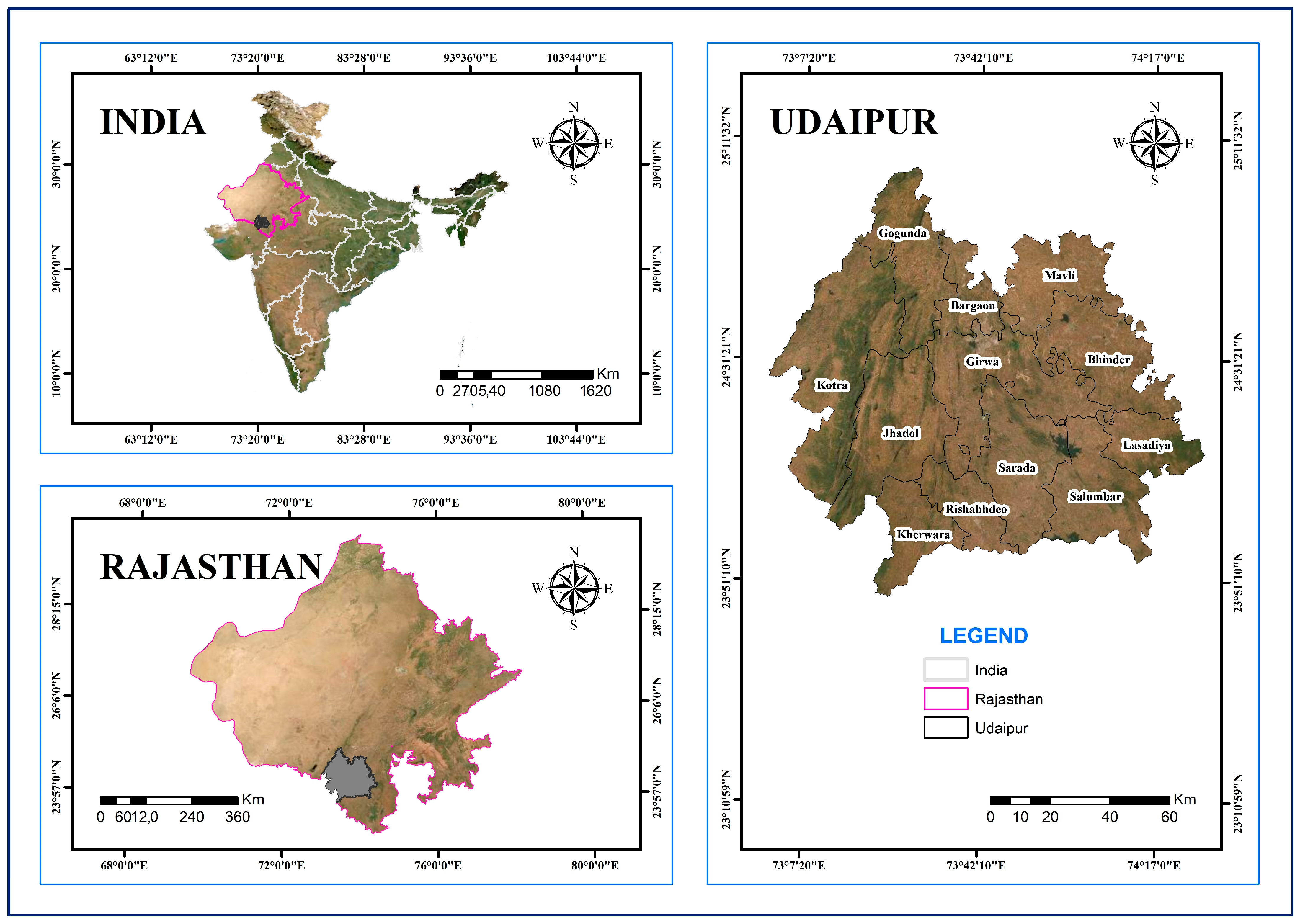
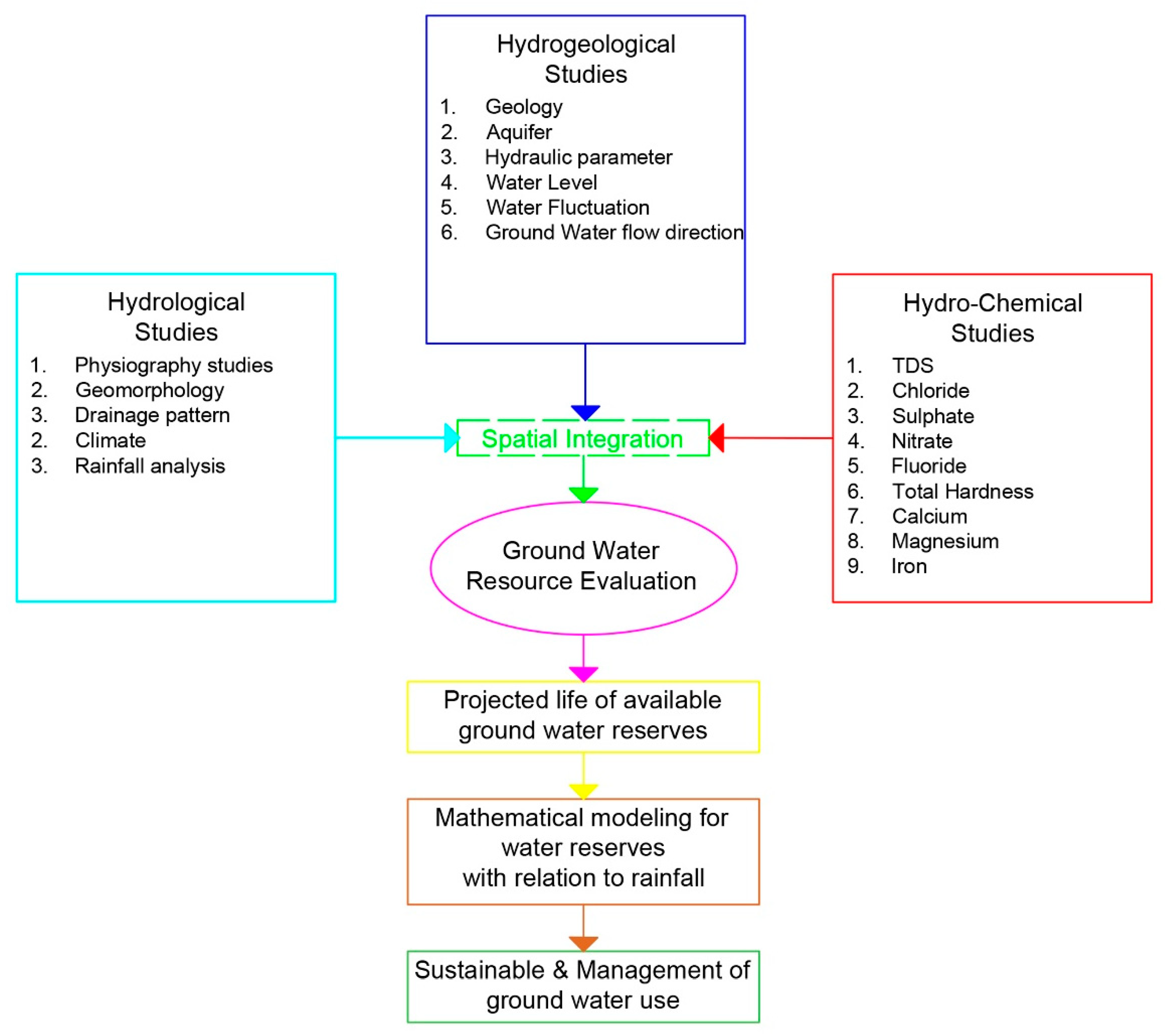
2. Materials and Methods
3. Results and Discussion
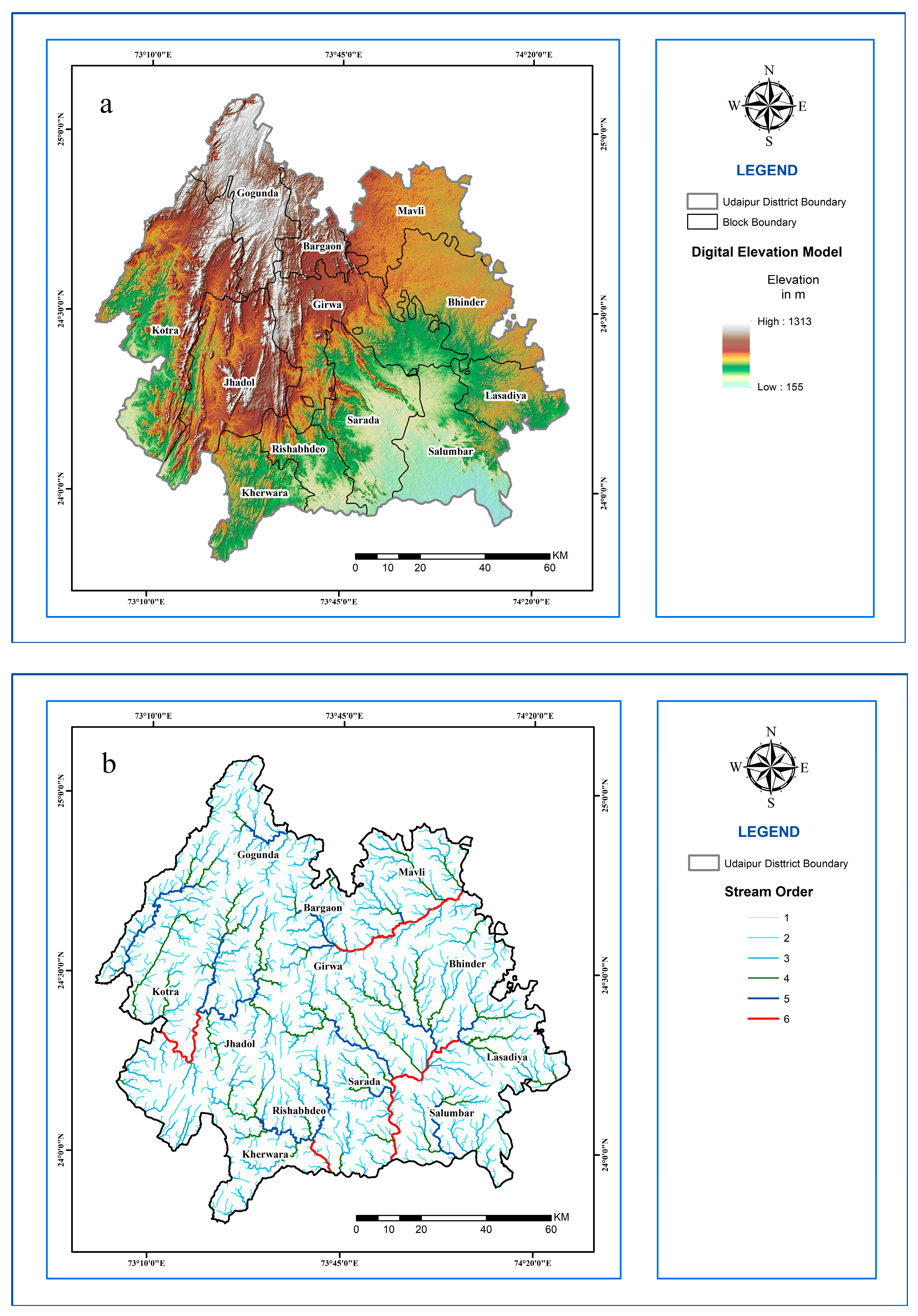
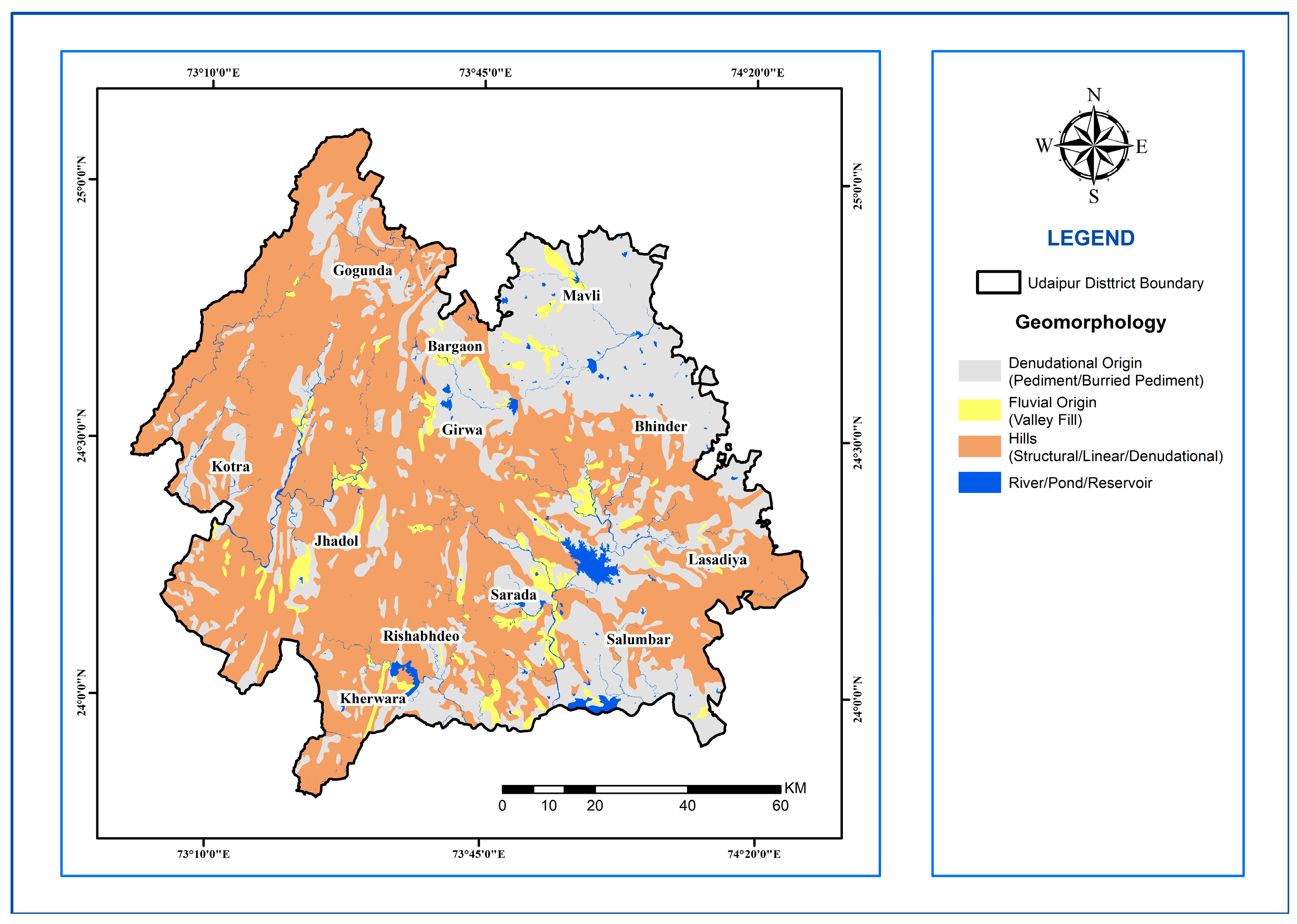
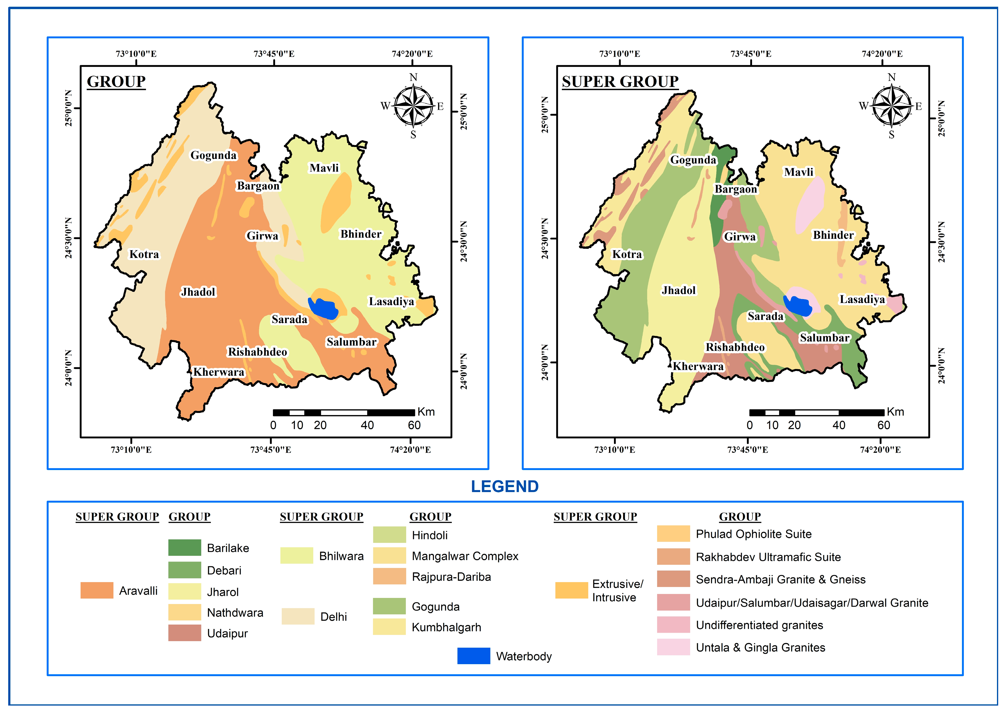
3.1. Geomorphological Characterization
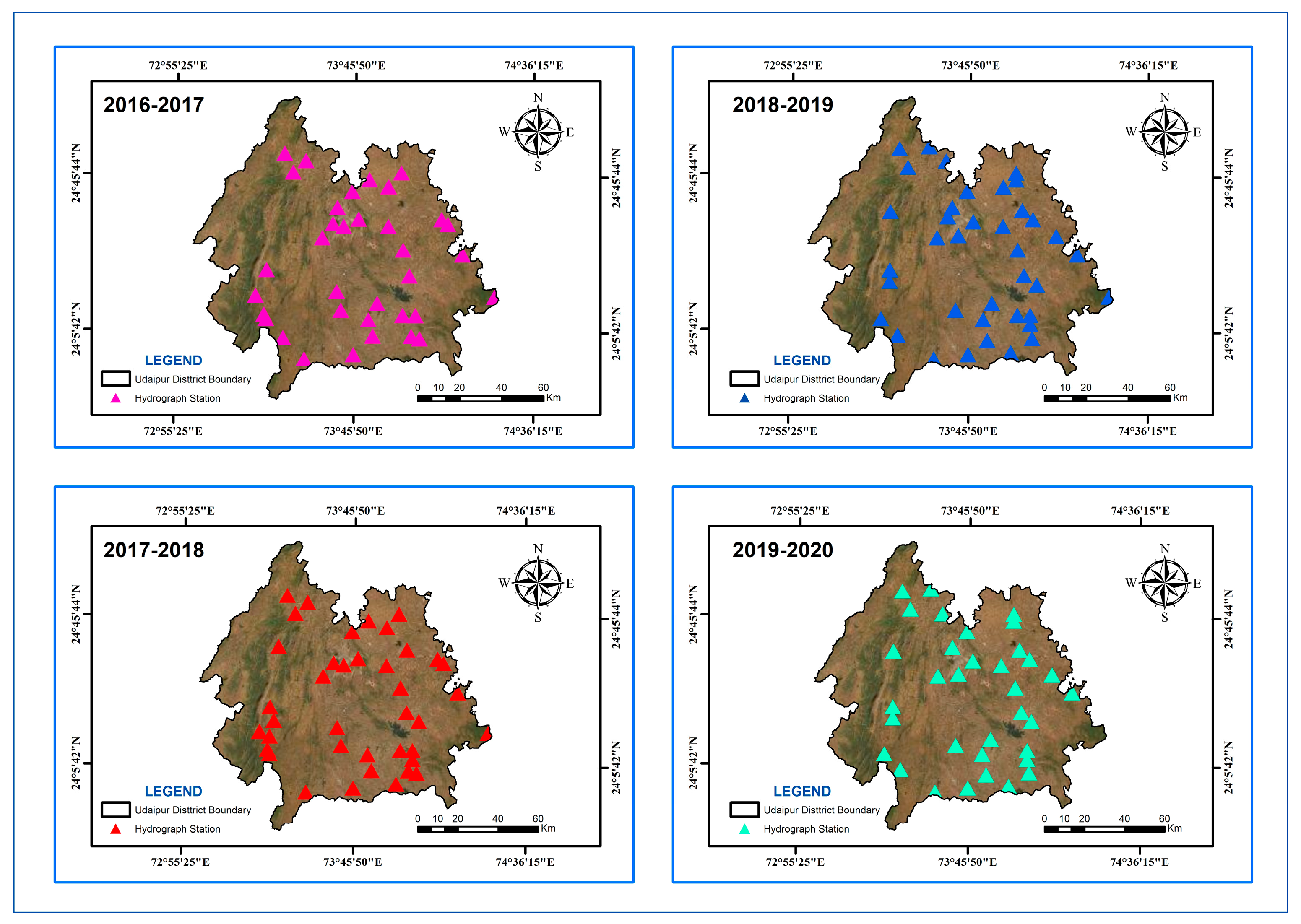
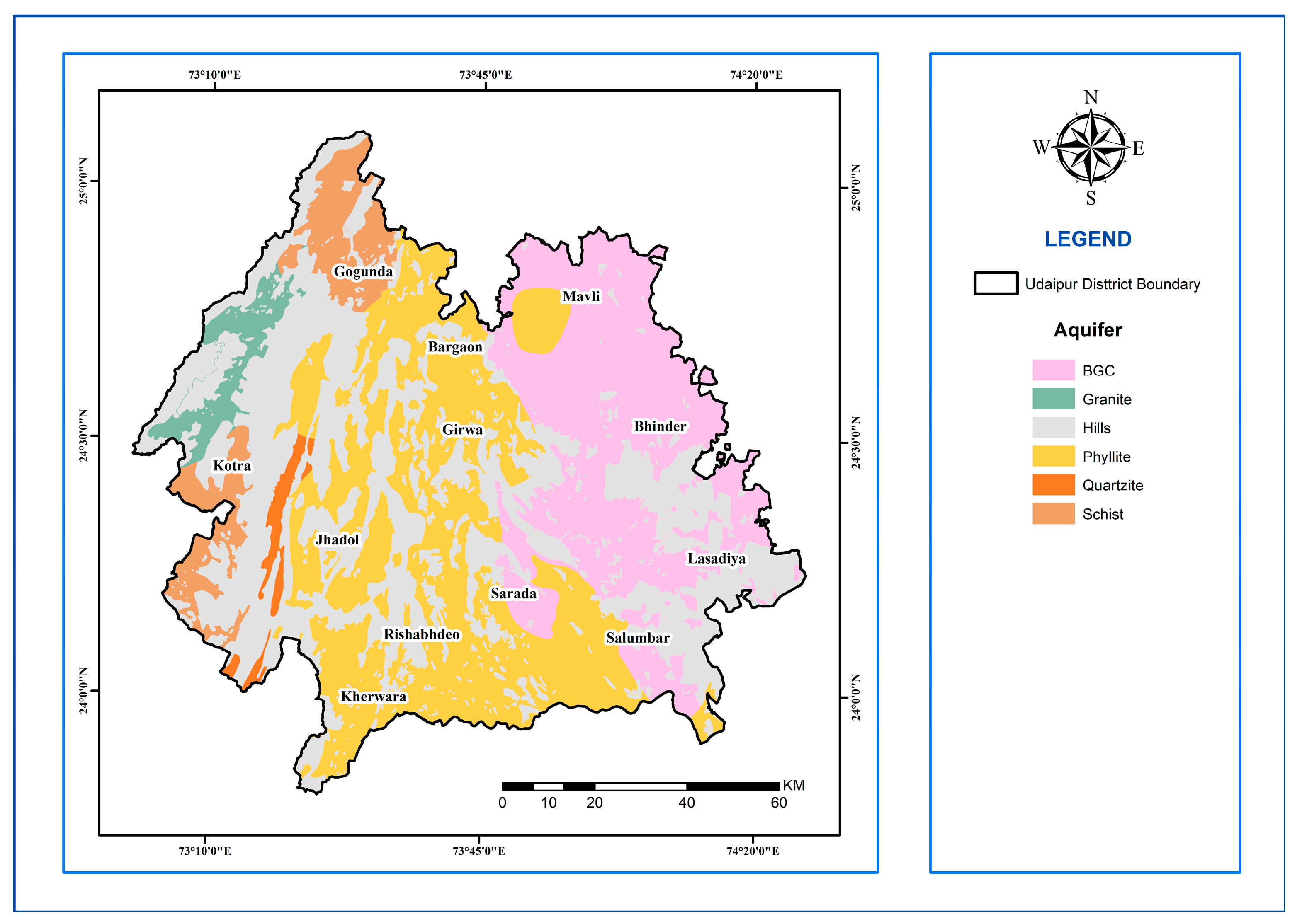
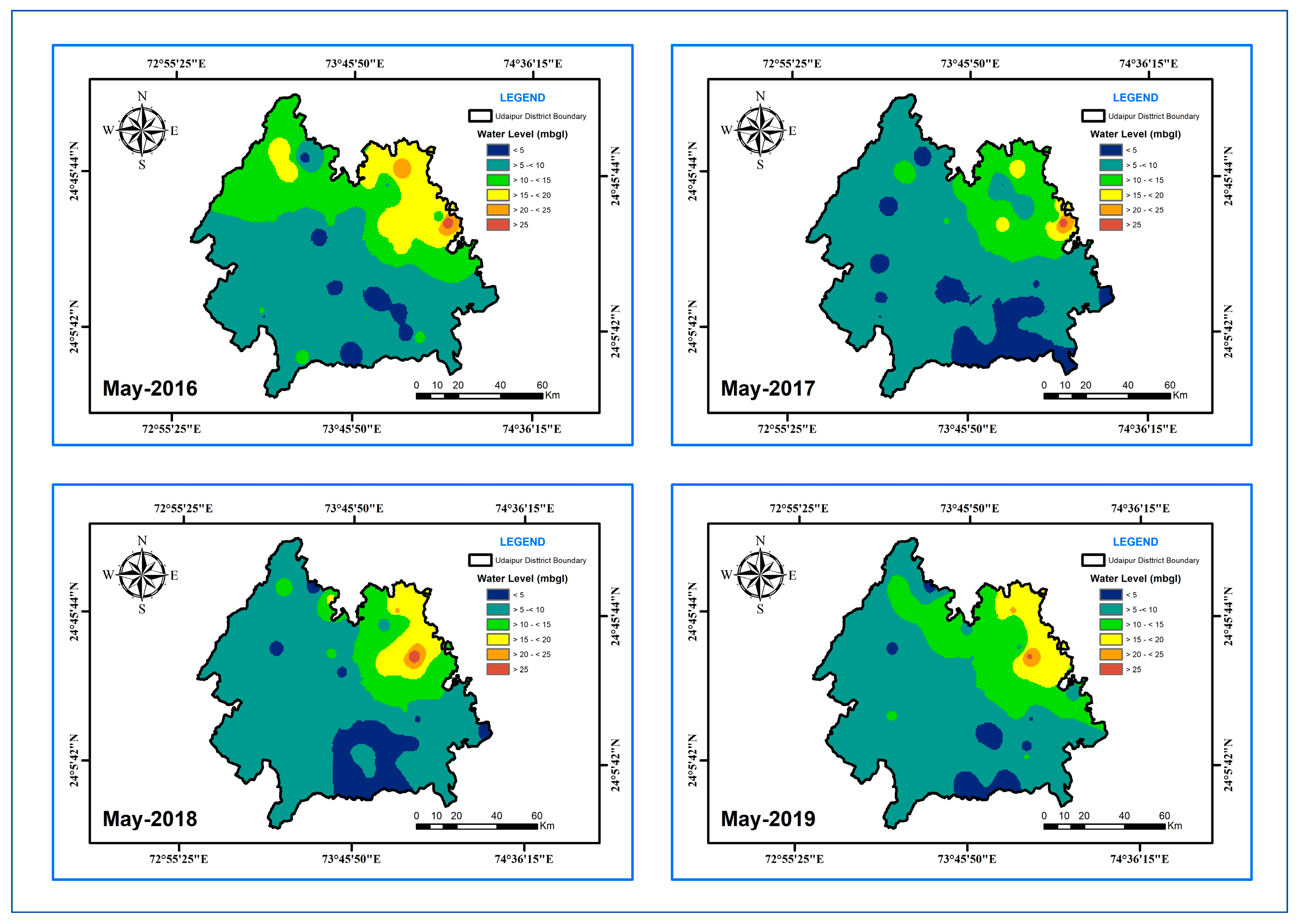
3.2. Hydrogeological Characterization
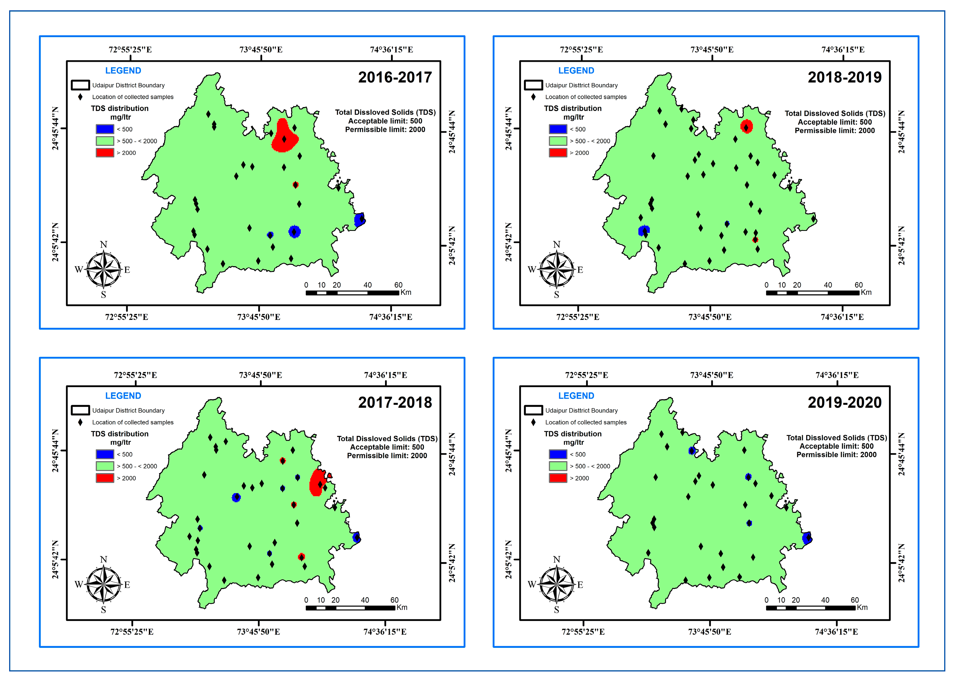
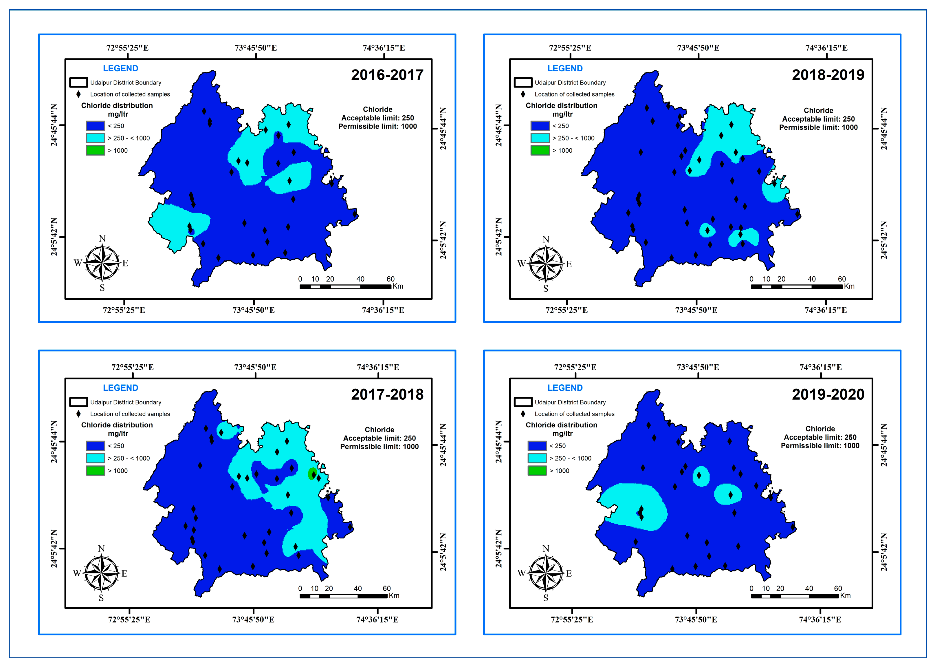
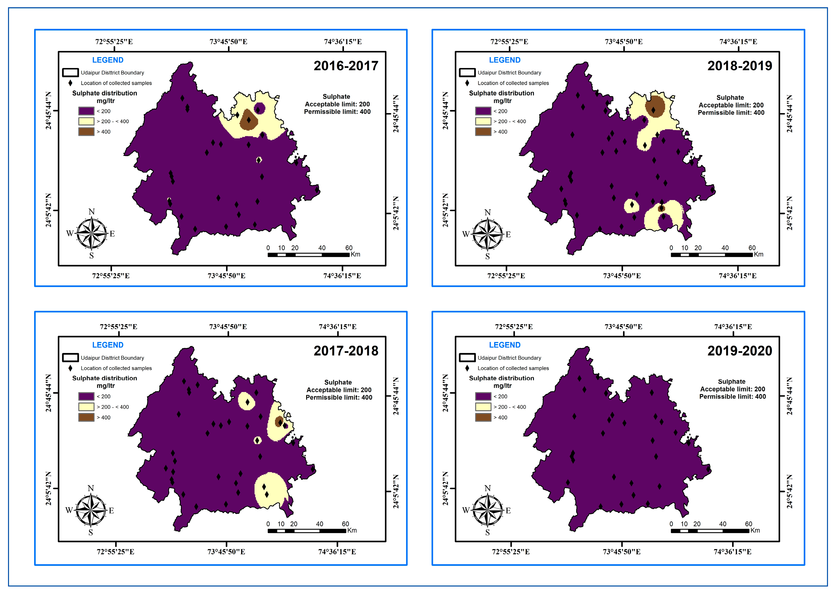
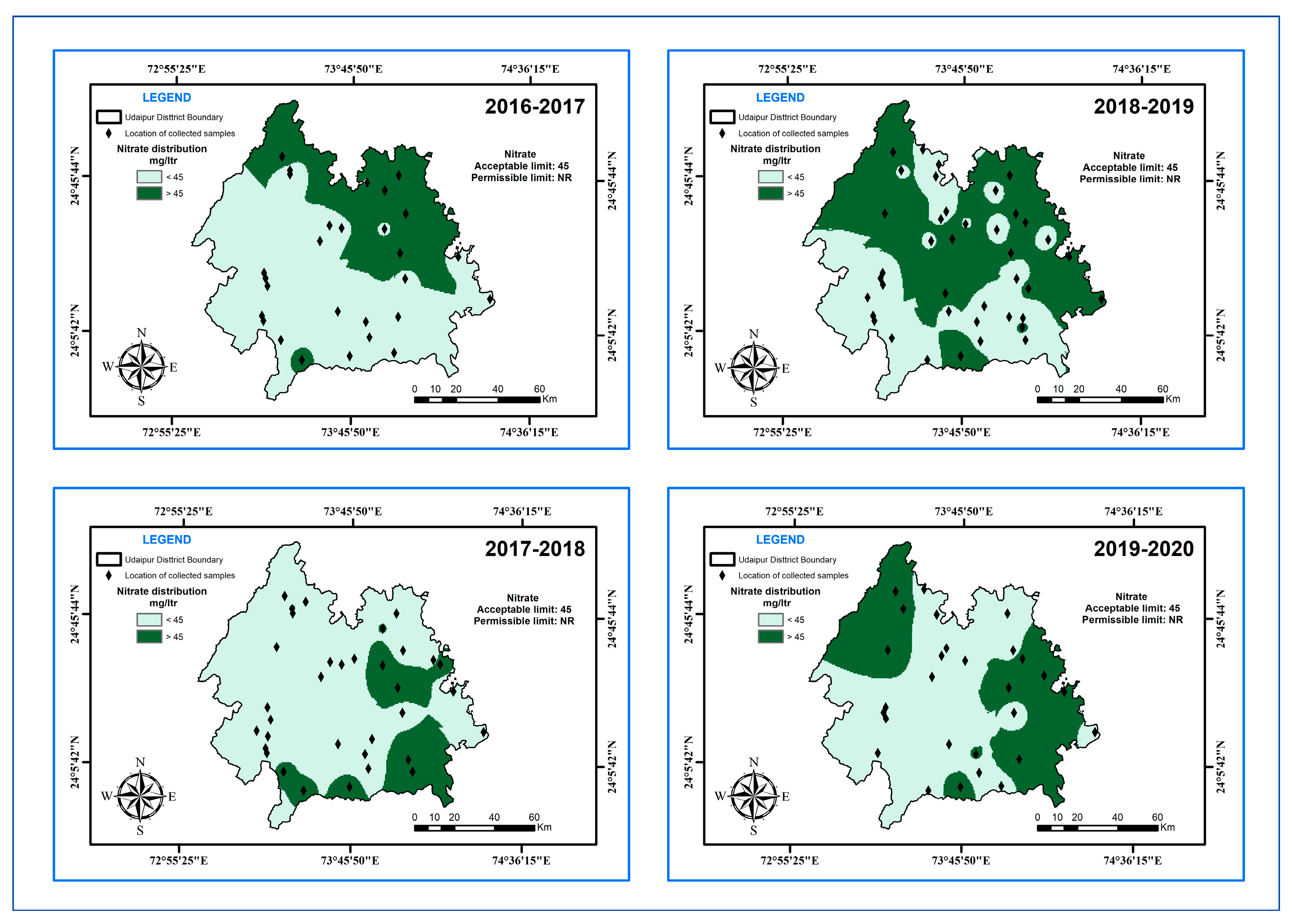
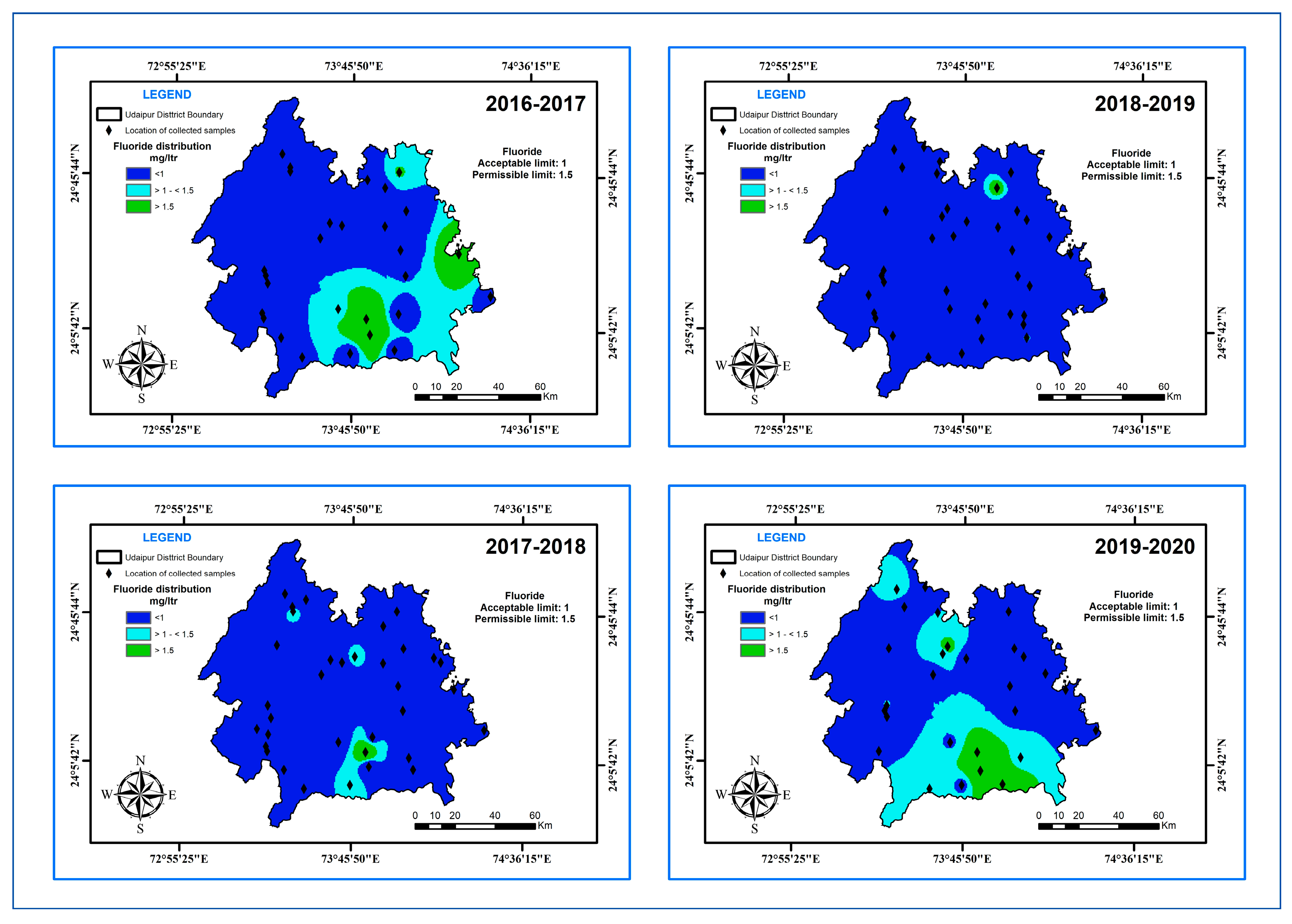
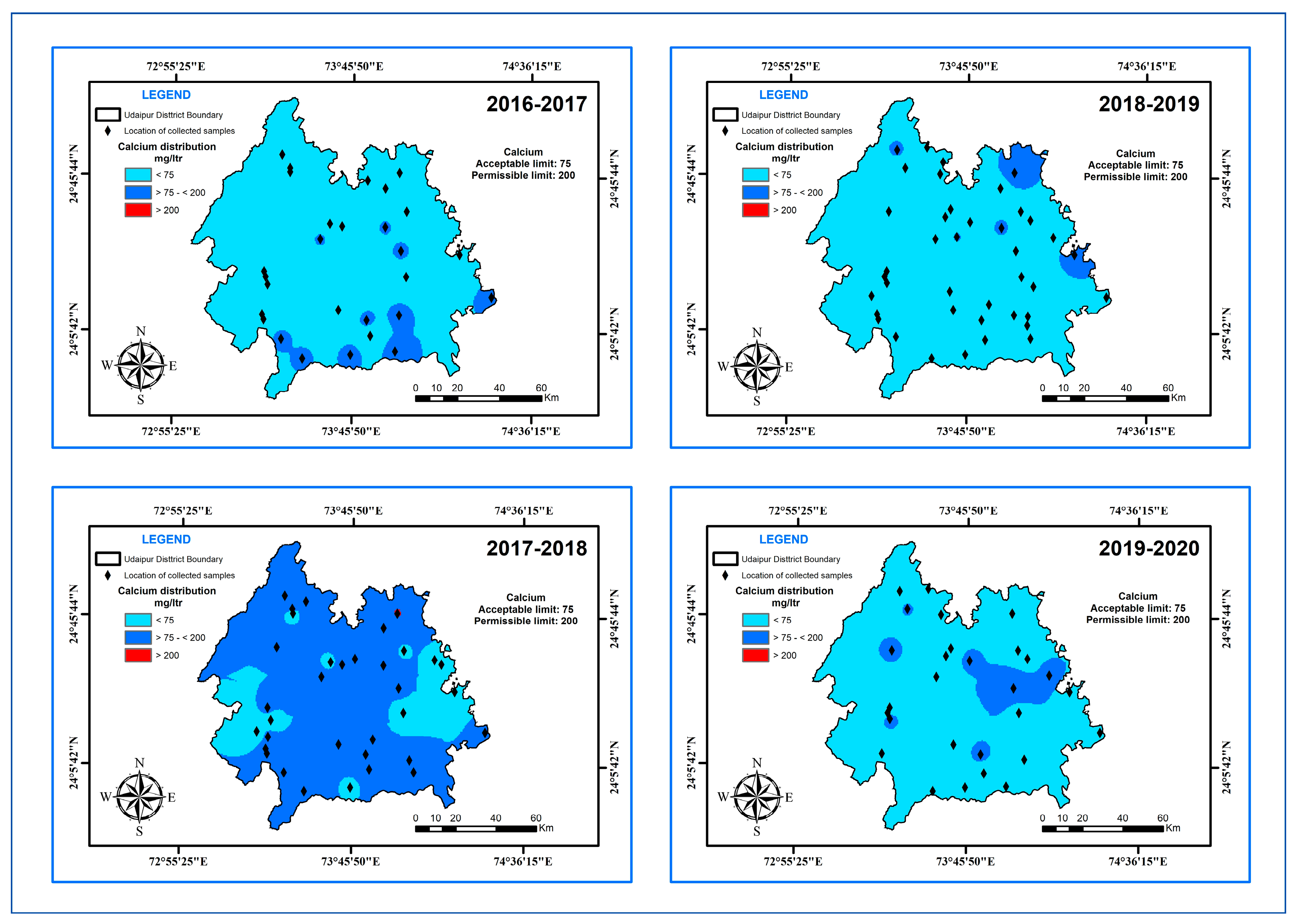
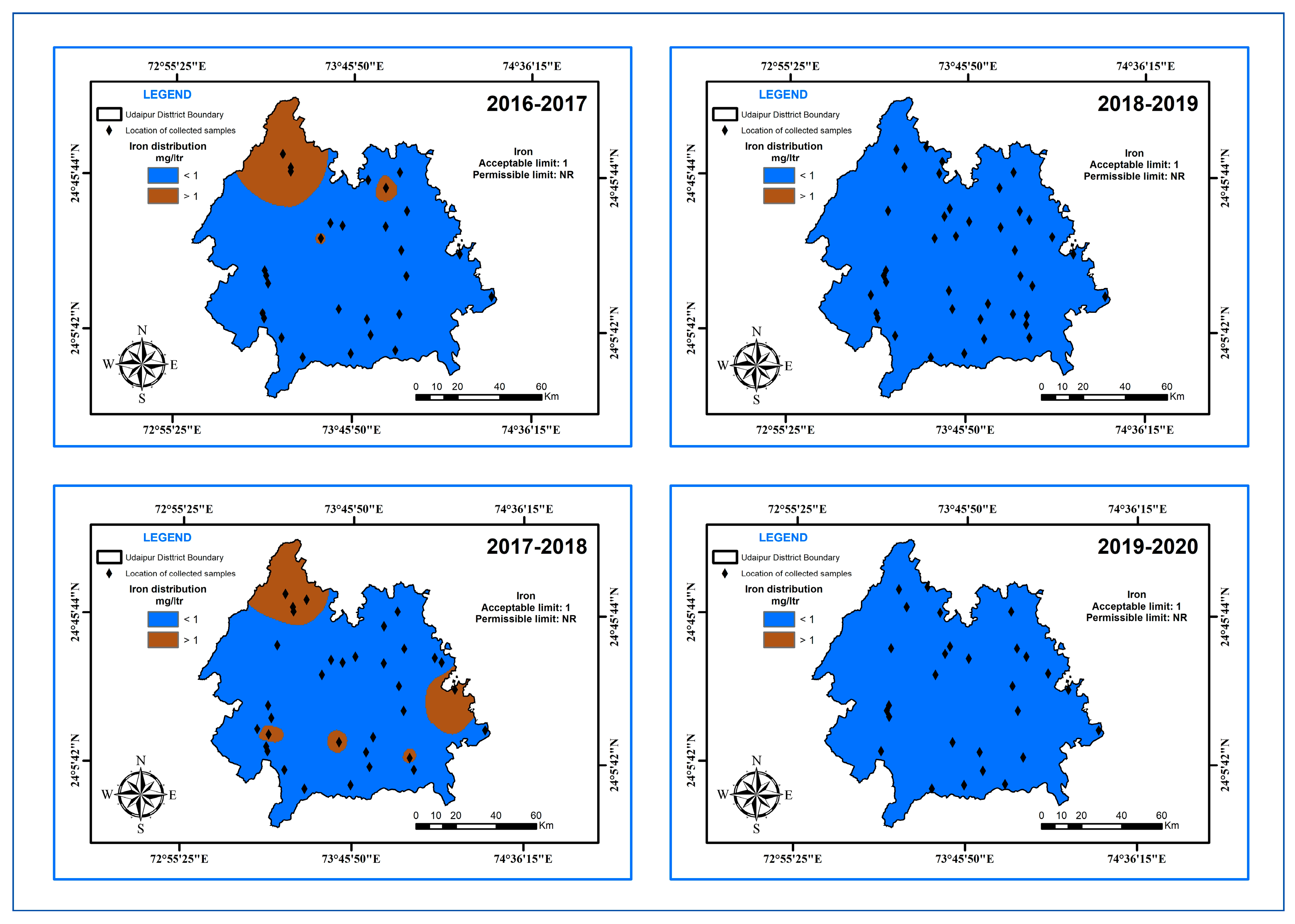
3.3. Hydrochemical Characterization
3.4. Groundwater Resource Evaluation
3.5. Projected Life of Reserves
3.6. Sustainability Management of Groundwater Reserves
4. Conclusions
Author Contributions
Funding
Institutional Review Board Statement
Informed Consent Statement
Data Availability Statement
Acknowledgments
Conflicts of Interest
References
- Shyam, G.M.; Taloor, A.K.; Singh, S.K.; Kanga, S. Sustainable Water Management using rainfall-runoff modelling: A geospatial approach. Groundw. Sustain. Dev. 2021, 15, 100676. [Google Scholar] [CrossRef]
- Haque, S.; Kannaujiya, S.; Taloor, A.K.; Keshri, D.; Bhunia, R.K.; Kumar, P.; Ray, C.; Chauhan, P. Identification of groundwater resource zone in the active tectonic region of Himalaya through earth observatory techniques. Groundw. Sustain. Dev. 2020, 10, 100337. [Google Scholar] [CrossRef]
- Khatri, N.; Tyagi, S. Influences of natural and anthropogenic factors on surface and groundwater quality in rural and urban areas. Front. Life Sci. 2015, 8, 23–39. [Google Scholar] [CrossRef]
- Kirmani, S.S. Water, peace and conflict management: The experience of the Indus and Mekong river basins. Water Int. 1990, 15, 200–205. [Google Scholar] [CrossRef]
- Gude, V.G.; Nirmalakhandan, N. Sustainable desalination using solar energy. Energy Convers. Manag. 2010, 51, 2245–2251. [Google Scholar] [CrossRef]
- Konikow, L.F. Long-term groundwater depletion in the United States. Groundwater 2015, 53, 2–9. [Google Scholar] [CrossRef] [PubMed]
- Balkhair, K.S.; Rahman, K.U. Development and assessment of rainwater harvesting suitability map using analytical hierarchy process, GIS and RS techniques. Geocarto Int. 2021, 36, 421–448. [Google Scholar] [CrossRef]
- El Raey, M. Mapping areas affected by sea-level rise due to climate change in the Nile delta until 2100. In Coping with Global Environmental Change, Disasters and Security; Springer: Berlin/Heidelberg, Germany, 2011; pp. 773–788. [Google Scholar]
- Taylor, R.G.; Scanlon, B.; Döll, P.; Rodell, M.; Van Beek, R.; Wada, Y.; Longuevergne, L.; Leblanc, M.; Famiglietti, J.S.; Edmunds, M.; et al. Ground water and climate change. Nat. Clim. Chang. 2013, 3, 322–329. [Google Scholar] [CrossRef] [Green Version]
- Bera, A.; Singh, S.K. Comparative assessment of livelihood vulnerability of climate induced migrants: A micro level study on Sagar Island, India. Sustain. Agri Food Environ. Res. 2021, 9, 1–15. [Google Scholar] [CrossRef]
- Etikala, B.; Adimalla, N.; Madhav, S.; Somagouni, S.G.; Keshava Kiran Kumar, P.L. Salinity Problems in Groundwater and Management Strategies in Arid and Semi-arid Regions. Groundw. Geochem. Pollut. Remediat. Methods 2021, 42–56. [Google Scholar] [CrossRef]
- Shah, T.; Roy, A.D.; Qureshi, A.S.; Wang, J. Sustaining Asia’s Groundwater Boom: An Overview of Issues and Evidence. Nat. Resour. Forum 2003, 27, 130–141. [Google Scholar] [CrossRef] [Green Version]
- Hayton, R.D.; Utton, A.E. Transboundary groundwaters: The Bellagio draft treaty. Nat. Resour. J. 1989, 29, 663. [Google Scholar]
- Sarkar, T.; Kannaujiya, S.; Taloor, A.K.; Kumar, P.; Ray, C.; Chauhan, P. Integrated study of GRACE data derived interannual groundwater storage variability over water stressed Indian regions. Groundw. Sustain. Dev. 2020, 10, 100376. [Google Scholar] [CrossRef]
- Singh, A.K.; Jasrotia, A.S.; Taloor, A.K.; Kotlia, B.S.; Kumar, V.; Roy, S.; Ray, P.K.C.; Singh, K.K.; Singh, A.K.; Sharma, A.K. Estimation of quantitative measures of total water storage variation from GRACE and GLDAS-NOAH satellites using geospatial technology. Quat. Int. 2017, 444, 191–200. [Google Scholar] [CrossRef]
- Shekhar, S.; Prasad, R.K. The groundwater in the Yamuna flood plain of Delhi (India) and the management options. Hydrogeol. J. 2009, 17, 1557. [Google Scholar] [CrossRef]
- Taloor, A.K.; Pir, R.A.; Adimalla, N.; Ali, S.; Manhas, D.S.; Roy, S.; Singh, A.K. Spring water quality and discharge assessment in the Basantar watershed of Jammu Himalaya using geographic information system (GIS) and water quality Index (WQI). Groundw. Sustain. Dev. 2020, 10, 100364. [Google Scholar] [CrossRef]
- Rao, S.V.N.; Kumar, S.; Shekhar, S.; Sinha, S.K.; Manju, S. Optimal pumping from skimming wells from the Yamuna River flood plain in north India. Hydrogeol. J. 2007, 15, 1157–1167. [Google Scholar] [CrossRef]
- Mirzadeh, S.M.J.; Jin, S.; Parizi, E.; Chaussard, E.; Bürgmann, R.; Delgado Blasco, J.M.; Amani, M.; Bao, H.; Mirzadeh, S.H. Characterization of Irreversible Land Subsidence in the Yazd-Ardakan Plain, Iran From 2003 to 2020 InSAR Time Series. J. Geophys. Res. Solid Earth 2021, 126, e2021JB022258. [Google Scholar] [CrossRef]
- Oude Essink, G.H. Salt water intrusion in a three-dimensional groundwater system in the Netherlands: A numerical study. Transp. Porous Media 2001, 43, 137–158. [Google Scholar] [CrossRef]
- Karanath, K.R. Groundwater Assessment, Development and Management; Tata McGraw Hill Pub. Co. Ltd.: New Delhi, India, 1987. [Google Scholar]
- Rahmati, O.; Pourghasemi, H.R.; Melesse, A.M. Application of GIS-based data driven random forest and maximum entropy models for groundwater potential mapping: A case study at Mehran Region, Iran. Catena 2016, 137, 360–372. [Google Scholar] [CrossRef]
- Lezzaik, K.; Milewski, A. A quantitative assessment of groundwater resources in the Middle East and North Africa region. Hydrogeol. J. 2018, 26, 251–266. [Google Scholar] [CrossRef]
- MacDonald, A.M.; Bonsor, H.C.; Dochartaigh, B.É.Ó.; Taylor, R.G. Quantitative maps of groundwater resources in Africa. Environ. Res. Lett. 2012, 7, 024009. [Google Scholar] [CrossRef]
- Singh, S.K.; Pandey, A.C. Geomorphology and the controls of geohydrology on waterlogging in Gangetic plains, North Bihar, India. Environ. Earth Sci. 2014, 71, 1561–1579. [Google Scholar] [CrossRef]
- Farooq, M.; Singh, S.K.; Kanga, S. Inherent vulnerability profiles of agriculture sector in temperate Himalayan region: A preliminary assessment. Indian J. Ecol. 2021, 48, 434–441. [Google Scholar]
- Kanga, S.; Meraj, G.; Das, B.; Farooq, M.; Chaudhuri, S.; Singh, S.K. Modeling the spatial pattern of sediment flow in lower Hugli estuary, West Bengal, India by quantifying suspended sediment concentration (SSC) and depth conditions using geoinformatics. Appl. Comput. Geosci. 2020, 8, 100043. [Google Scholar] [CrossRef]
- Narasimha Prasad, N.B.; Shivraj, P.V.; Jagatheesan, M.S. Evaluation of Groundwater Development Prospects in Kadalundi River Basin. J. Geol. Soc. India 2007, 69, 1103–1110. [Google Scholar]
- Jeelani, G. Aquifer response to regional climate variability in a part of Kashmir Himalaya in India. Hydrogeol. J. 2008, 16, 1625–1633. [Google Scholar] [CrossRef]
- Shah, T. Towards a Managed Aquifer Recharge strategy for Gujarat, India: An economist’s dialogue with hydro-geologists. J. Hydrol. 2014, 518, 94–107. [Google Scholar] [CrossRef]
- Meraj, G.; Singh, S.K.; Kanga, S.; Islam, M.N. Modeling on comparison of ecosystem services concepts, tools, methods and their ecological-economic implications: A review. Model. Earth Syst. Environ. 2021. [Google Scholar] [CrossRef]
- Meraj, G.; Farooq, M.; Singh, S.K.; Islam, M.; Kanga, S. Modeling the sediment retention and ecosystem provisioning services in the Kashmir valley, India, Western Himalayas. Model. Earth Syst. Environ. 2021. [Google Scholar] [CrossRef]
- Pandey, A.C.; Singh, S.K.; Nathawat, M.S. Analysing the impact of anthropogenic activities on waterlogging dynamics in Indo-Gangetic plains, Northern Bihar, India. Int. J. Rem. Sens. 2012, 33, 135–149. [Google Scholar] [CrossRef]
- Zarghami, M.; Akbariyeh, S. System dynamics modeling for complex urban water systems: Application to the city of Tabriz, Iran. Resour. Conserv. Recycl. 2012, 60, 99–106. [Google Scholar] [CrossRef]
- Kumar, R.; Singh, R.D.; Sharma, K.D. Water resources of India. Curr. Sci. 2005, 5, 794–811. [Google Scholar]
- Hu, X.; Shi, L.; Zeng, J.; Yang, J.; Zha, Y.; Yao, Y.; Cao, G. Estimation of actual irrigation amount and its impact on groundwater depletion: A case study in the Hebei Plain, China. J. Hydrol. 2016, 543, 433–449. [Google Scholar] [CrossRef]
- Dangar, S.; Asoka, A.; Mishra, V. Causes and implications of groundwater depletion in India: A review. J. Hydrol. 2021, 596, 126103. [Google Scholar] [CrossRef]
- Moore, I.D.; Grayson, R.B.; Ladson, A.R. Digital terrain modelling: A review of hydrological, geomorphological, and biological applications. Hydrol. Processes 1991, 5, 3–30. [Google Scholar] [CrossRef]
- Fenta, A.A.; Kifle, A.; Gebreyohannes, T.; Hailu, G. Spatial analysis of groundwater potential using remote sensing and GIS-based multi-criteria evaluation in Raya Valley, northern Ethiopia. Hydrogeol. J. 2015, 23, 195–206. [Google Scholar] [CrossRef]
- Portoghese, I.; Uricchio, V.; Vurro, M. A GIS tool for hydrogeological water balance evaluation on a regional scale in semi-arid environments. Comput. Geosci. 2005, 31, 15–27. [Google Scholar] [CrossRef]
- Wałęga, A.; Młyński, D.; Wojkowski, J.; Radecki-Pawlik, A.; Lepeška, T. New empirical model using landscape hydric potential method to estimate median peak discharges in mountain ungauged catchments. Water 2020, 12, 983. [Google Scholar] [CrossRef] [Green Version]
- Espinha Marques, J.; Samper, J.; Pisani, B.; Alvares, D.; Carvalho, J.M.; Chaminé, H.I.; Marques, J.M.; Vieira, G.T.; Mora, C.; Sodré Borges, F. Evaluation of water resources in a high-mountain basin in Serra da Estrela, Central Portugal, using a semi-distributed hydrological model. Environ. Earth Sci. 2011, 62, 1219–1234. [Google Scholar] [CrossRef]
- Mussa, K.R.; Mjemah, I.C.; Machunda, R.L. Open-source software application for hydrogeological delineation of potential groundwater recharge zones in the singida semi-arid, fractured aquifer, Central Tanzania. Hydrology 2020, 7, 28. [Google Scholar] [CrossRef]
- Asadi, H.; Shahedi, K.; Jarihani, B.; Sidle, R.C. Rainfall-runoff modelling using hydrological connectivity index and artificial neural network approach. Water 2019, 11, 212. [Google Scholar] [CrossRef] [Green Version]
- Arabi, M.; Govindaraju, R.S.; Hantush, M.M. A probabilistic approach for analysis of uncertainty in the evaluation of watershed management practice. J. Hydrol. 2007, 333, 459–471. [Google Scholar] [CrossRef]
- Singh, P.K.; Dahiphale, P.; Yadav, K.K.; Singh, M. Delineation of groundwater potential zones in Jaisamand basin of Udaipur district. In Groundwater; Springer: Singapore, 2018; pp. 3–20. [Google Scholar]
- Roy, A.B.; Paliwal, B.S. Evolution of lower Proterozoic epicontinental deposits: Stromatolite-bearing Aravalli rocks of Udaipur, Rajasthan, India. Precambrian Res. 1981, 14, 49–74. [Google Scholar] [CrossRef]
- Central Ground Water Board (CGWB). Manual on Artificial Recharge of Groundwater; Ministry of Water Resources, Government of India: New Delhi, India, 2007. [Google Scholar]
- Gong, G.; Mattevada, S.; O’Bryant, S.E. Comparison of the accuracy of kriging and IDW interpolations in estimating groundwater arsenic concentrations in Texas. Environ. Res. 2014, 130, 59–69. [Google Scholar] [CrossRef]
- Luo, W.; Taylor, M.C.; Parker, S.R. A comparison of spatial interpolation methods to estimate continuous wind speed surfaces using irregularly distributed data from England and Wales. Int. J. Climatol. J. R. Meteorol. Soc. 2008, 28, 947–959. [Google Scholar] [CrossRef]
- Nawar, S.; Corstanje, R.; Halcro, G.; Mulla, D.; Mouazen, A.M. Delineation of soil management zones for variable-rate fertilization: A review. Adv. Agron. 2017, 143, 175–245. [Google Scholar]
- Kanga, S.; Sudhanshu Meraj, G.; Farooq, M.; Nathawat, M.S.; Singh, S.K. Reporting the management of COVID-19 threat in India using remote sensing and GIS based approach. Geocarto Int. 2020, 1–8. [Google Scholar] [CrossRef]
- Kanga, S.; Meraj, G.; Farooq, M.; Nathawat, M.S.; Singh, S.K. Analyzing the risk to COVID-19 infection using remote sensing and GIS. Risk Anal. 2021, 41, 801–813. [Google Scholar] [CrossRef] [PubMed]
- Tomar, P.; Singh, S.K.; Kanga, S.; Meraj, G.; Kranjčić, N.; Đurin, B.; Pattanaik, A. GIS-Based Urban Flood Risk Assessment and Management—A Case Study of Delhi National Capital Territory (NCT), India. Sustainability 2021, 13, 12850. [Google Scholar] [CrossRef]
- Meraj, G. Ecosystem service provisioning–underlying principles and techniques. SGVU J. Clim. Chang. Water 2020, 7, 56–64. [Google Scholar]
- Pall, I.A.; Meraj, G.; Romshoo, S.A. Applying integrated remote sensing and field- based approach to map glacial landform features of the Machoi Glacier valley, NW Himalaya. SN Appl. Sci. 2019, 1, 488. [Google Scholar] [CrossRef] [Green Version]
- Singh, S.; Raju, N.J.; Ramakrishna, C. Evaluation of groundwater quality and its suitability for domestic and irrigation use in parts of the Chandauli-Varanasi region, Uttar Pradesh, India. J. Water Resour. Prot. 2015, 7, 572. [Google Scholar] [CrossRef] [Green Version]
- Chinnasamy, P.; Maheshwari, B.; Prathapar, S. Understanding groundwater storage changes and recharge in Rajasthan, India through remote sensing. Water 2015, 7, 5547–5565. [Google Scholar] [CrossRef] [Green Version]
- Groundwater Resource Estimation Committee (GEC). Ground Water Resource Estimation Methodology; India Ministry of Water Resources Report; India Ministry of Water Resources: Delhi, India, 2009; p. 107. [Google Scholar]
- Maheshwari, B.; Varua, M.; Ward, J.; Packham, R.; Chinnasamy, P.; Dashora, Y.; Dave, S.; Soni, P.; Dillon, P.; Purohit, R.; et al. The Role of Transdisciplinary Approach and Community Participation in Village Scale Groundwater Management: Insights from Gujarat and Rajasthan, India. Water 2014, 6, 3386–3408. [Google Scholar] [CrossRef] [Green Version]
- Vikas, C.; Kushwaha, R.; Ahmad, W.; Prasannakumar, V.; Reghunath, R. Genesis and geochemistry of high fluoride bearing groundwater from a semi-arid terrain of NW India. Environ. Earth Sci. 2013, 68, 289–305. [Google Scholar] [CrossRef]
- Bhattacharjee, S.; Nandy, S. Geology of the western Arunachal Himalaya in parts of Tawang and West Kameng districts, Arunachal Pradesh. J. Geol. Soc. India 2008, 72, 199–207. [Google Scholar] [CrossRef]
- Bhattacharya, A.K. Artificial ground water recharge with a special reference to India. Int. J. Res. Rev. Appl. Sci. 2010, 4, 214–221. [Google Scholar]
- Kumari, P.; Kumar, G.; Prasher, S.; Kaur, S.; Mehra, R.; Kumar, P.; Kumar, M. Evaluation of uranium and other toxic heavy metals in drinking water of Chamba district, Himachal Pradesh, India for possible health hazards. Environ. Earth Sci. 2021, 80, 271. [Google Scholar] [CrossRef]
- Ibrahim, S.A.; Al-Tawash, B.S.; Abed, M.F. Environmental assessment of heavy metals in surface and groundwater at Samarra City, Central Iraq. Iraqi J. Science 2018, 59, 1277–1284. [Google Scholar]
- Takeuchi, K. Regional Water Exchange for Drought Alleviation. Doctoral Dissertation, Colorado State University, Fort Collins, CO, USA, 1974. [Google Scholar]
- Zhang, Y.; Chiew, F.H.S.; Zhang, L.; Li, H. Use of remotely sensed actual evapotranspiration to improve rainfall–runoff modelling in southeast Australia. J. Hydrometeorol. 2009, 10, 969–980. [Google Scholar] [CrossRef]
- Kwon, M.; Kwon, H.H.; Han, D. A hybrid approach combining conceptual hydrological models, support vector machines and remote sensing data for rainfall-runoff modeling. Rem. Sens. 2020, 12, 1801. [Google Scholar] [CrossRef]
- Hamdan, A.N.A.; Almuktar, S.; Scholz, M. Rainfall-runoff modeling using the HEC-HMS model for the Al-Adhaim River catchment, Northern Iraq. Hydrology 2021, 8, 58. [Google Scholar] [CrossRef]
- ASCE Manual. Groundwater Management; American Society of Civil Engineers: New York, NY, USA, 1987. [Google Scholar]
- Ibrahim, A.; Zakaria, N.; Harun, N.; Muzamil, M.; Hashim, M. Rainfall runoff modeling for the basin in Bukit Kledang, perak. In IOP Conference Series: Materials Science and Engineering, Proceedings of the International Nuclear Science Technology and Engineering Conference 2020 (iNuSTEC 2020), Selangor, Malaysia, 17–19 November 2020; IOP Publishing Ltd.: Bristol, UK, 2021; Volume 1106, p. 012033. [Google Scholar] [CrossRef]
- Shah, T.; Molden, D.; Sakthivadivel, R.; Seckler, D. Global groundwater situation: Opportunities and challenges. Econ. Political Wkly. 2001, 36, 4142–4150. [Google Scholar]
- Narasimha Prasad, N.B.; Sharma, K.K. Geophysical Investigations for Groundwater Exploration in Amini Island. Bull. Pure Appl. Sci. 2003, 22, 31–41. [Google Scholar]
- Narasimha Prasad, N.B. Assessment of Groundwater Resources in Nileshwar Basin. J. Appl. Hydrol. 2003, XVI, 52–60. [Google Scholar]
- Wali, S.U.; Abubakar, I.M.; Umar, M.A.; Shera, A.A. Reassessing Groundwater Potentials and Subsurface water Hydro-chemistry in a Tropical Anambra Basin, Southeastern Nigeria. J. Geol. Res. 2020, 2, 1–24. [Google Scholar] [CrossRef]
- Boryczko, K.; Rak, J. Method for assessment of water supply diversification. Resources 2020, 9, 87. [Google Scholar] [CrossRef]
- India Meteorological Department (IMD). Meteorological monograph: Hydrology N0. In Rainfall Profile of Udaipur; 15/2013; Meteorological Centre, Jaipur & Meteorological Department: New Delhi, India, 2013; pp. 1–113. [Google Scholar]
- Chatterjee, R.; Gupta, B.K.; Mohiddin, S.K.; Singh, P.N.; Shekhar, S.; Purohit, R. Dynamic groundwater resources of National Capital Territory, Delhi: Assessment, development and management options. Environ. Earth Sci. 2009, 59, 669–686. [Google Scholar] [CrossRef]
- Shin, S.; Park, H. Achieving cost-efficient diversification of water infrastructure system against uncertainty using modern portfolio theory. J. Hydroinform. 2018, 20, 739–750. [Google Scholar] [CrossRef]
- Shekhar, S. An approach to interpretation of step drawdown tests. Hydrogeol. J. 2006, 14, 1018–1027. [Google Scholar] [CrossRef]
- Shekhar, S.; Purohit, R.; Kaushik, Y.B. Groundwater management in NCT Delhi, Technical paper included in the special session on Ground water. In Proceedings of the 5th Asian Regional Conference of INCID, Vegan Bhawan, New Delhi, India, 9–11 December 2009; Available online: https://www.researchgate.net/publication/238708371_Groundwater_Management_in_NCT_Delhi (accessed on 31 December 2021).


| Dynamic Reserves (RT) | Rr + RR + Rp + Ri | |
|---|---|---|
| Where | Rr = Recharge due to rainfall | Rr = A × S.F. × Sy Rr = Recharge due to Rainfall A = Total rechargeable area S.F. = Average Seasonal Fluctuation in the studied area Sy = Specific Yield |
| RR = Recharge due to river | T × ΔH/ΔI × L × no. of days T = Transmissivity (As per APT results) ΔH/ΔI = Hydraulic Gradient (As per Water-Level Contour Map) L = length of river section, No. of days of river flow as reported in field = 30 days | |
| Rp = recharge due to ponds | Spread area of pond × Seepage factor × No. of days of water storage Seepage rate = 1.4 mm/day = 0.0014 m/day (As per GEC) | |
| Ri = recharge due to applied irrigation | Irrigated area (As per collected data from Revenue Department of Jaitaran and Raipur) × Recharge factor for Paddy/Non-Paddy | |
| Groundwater Draft (DT) | Dd + Di + DI + De | |
| Where | Draft due to domestic consumption (Dd) | Population × Water requirement per day in m3 × no. of days |
| Draft due to applied irrigation (Di) | Average irrigated area × Average crop factor for general mixed crops | |
| Draft due to Industrial consumption (DI) | Water requirement per day in m3 × no. of days | |
| Draft due to natural outflow (Do) | Do = T × ΔH/ΔI × L × No. of days in a year T = Average Transmissivity of all aquifers ΔH/ΔI = Average Hydraulic Gradient L = Length of out flow boundary | |
| Draft due to Evapotranspiration (De) | Replenishable reserves × Evapotranspiration Factor | |
| Surplus/Deficit Reserves | Total dynamic groundwater reserves–Total present groundwater draft | |
| Stage of Groundwater Development | Total groundwater Draft × 100 Total groundwater reserves | |
| Static Reserves (Sr) | A × S.T. × Sy where A = Area of different aquifers S.T. = Average saturated thickness | |
| Age | Super Group | Group | Lithology |
|---|---|---|---|
| Palaeoproterozoic | Aravalli | Barilake | Meta volcanics, chlorite schists, amphibolite, quartzite, and conglomerate |
| Debari | Meta arkose, quartzite, phyllite, dolomitic marble, and dolomite | ||
| Jharol | Chlorite-mica schist, calc shist, and quartzite | ||
| Nathdwara | Banded gneissic complex (BGC) | ||
| Udaipur | Phyllite, mica schists, meta siltstone, quartzite, dolomite, gneisses and migmatites | ||
| Palaeoproterozoic | Bhiwara | Rajpura-Dariba | Meta-volcano-sedimentory rocks of banded gneissic complex (BGC) |
| Palaeoproterozoic–Mesoproterozoic | Delhi | Gogunda | Calc schist, gneisses, mica shists, garnetiferous biotite-schists, quartzites, and migmatites |
| Kumbhalgarh | Carbonate, mafic volcanic, and argillaceous rocks | ||
| Palaeoproterozoic–Mesoproterozoic | Extrusive/ Intrusive | Phulad Ophiolite Suite | Banded gneissic complex (BGC) |
| Palaeoproterozoic | Rakhabdev Ultramafic Suite | Serpentinite, talc-chlorite-schist, actinolite-tremolite schist, and asbestos | |
| Mesoproterozoic | Sendra-Ambaji Granite and Gneiss | Schists, gneisses, and composite gneiss Quartzites | |
| Palaeoproterozoic | Udaipur/Salumbar/Udaisagar/Darwal Granite | ||
| - | Undifferentiated Granite | ||
| --------------------------------------------------Unconformity-------------------------------------------------- | |||
| Archaean | Bhiwara | Hindoli | - |
| Mangalwar Complex | Migmatites, gneisses, quartzite, felspathic granite ferrous mica shists and para-amphibolites | ||
| - | Extrusive/ Intrusive | Untala and Gingla Granites | Politic gneiss, quartzite, marble, calc-silicates |
| Type of Aquifer | Name of the Location | Yield Range in m3/day | Depth Range of Groundwater Abstraction Structure in m |
|---|---|---|---|
| Calc schist and gneiss | Gogunda | 40–60 | 15–20 |
| Kotra | 40–50 | 15–20 | |
| Granite | Kotra | 35–50 | 15–20 |
| Quartzite | Jhadol | 25–35 | 20–25 |
| Phyllite and schist | Bargaon | 40–60 | 15–20 |
| Girwa | 50–80 | 25–30 | |
| Gogunda | 50–80 | 20–25 | |
| Jhadol | 40–60 | 25–30 | |
| Kherwara | 40–60 | 20–25 | |
| Kotra | 40–60 | 20–25 | |
| Mavli | 40–60 | 25–30 | |
| Salumbar | 40–60 | 15–20 | |
| Sarada | 40–60 | 15–20 | |
| Granites and gneiss | Bhinder | 35–50 | 15–20 |
| Sarada | 35–45 | 15–20 | |
| Salumbar | 35–45 | 20–25 | |
| Mavli | 35–45 | 20–30 | |
| Girwa | 35–45 | 20–25 |
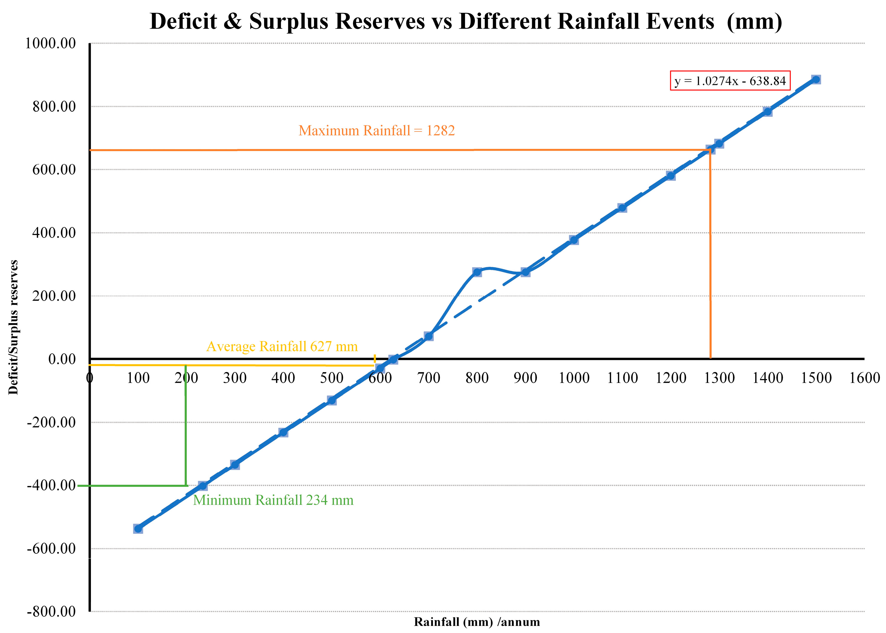
| Rainfall in mm/annum (X) | Dynamic Reserves in mcm/annum | Groundwater Draft in mcm/annum | Total Deficit/Surplus Reserves in mcm/annum (Y) |
|---|---|---|---|
| 100 | 101.66 | 639.67 | −538.01 |
| 200 | 203.32 | 639.67 | −436.35 |
| 300 | 304.99 | 639.67 | −334.68 |
| 400 | 406.65 | 639.67 | −233.02 |
| 500 | 508.31 | 639.67 | −131.36 |
| 600 | 609.97 | 639.67 | −29.70 |
| 627 | 637.42 | 639.67 | −2.25 |
| 700 | 711.63 | 639.67 | 71.96 |
| 800 | 914.96 | 639.67 | 275.29 |
| 900 | 914.96 | 639.67 | 275.29 |
| 1000 | 1016.62 | 639.67 | 376.95 |
| 1100 | 1118.28 | 639.67 | 478.61 |
| 1200 | 1219.94 | 639.67 | 580.27 |
Publisher’s Note: MDPI stays neutral with regard to jurisdictional claims in published maps and institutional affiliations. |
© 2022 by the authors. Licensee MDPI, Basel, Switzerland. This article is an open access article distributed under the terms and conditions of the Creative Commons Attribution (CC BY) license (https://creativecommons.org/licenses/by/4.0/).
Share and Cite
Shyam, M.; Meraj, G.; Kanga, S.; Sudhanshu; Farooq, M.; Singh, S.K.; Sahu, N.; Kumar, P. Assessing the Groundwater Reserves of the Udaipur District, Aravalli Range, India, Using Geospatial Techniques. Water 2022, 14, 648. https://doi.org/10.3390/w14040648
Shyam M, Meraj G, Kanga S, Sudhanshu, Farooq M, Singh SK, Sahu N, Kumar P. Assessing the Groundwater Reserves of the Udaipur District, Aravalli Range, India, Using Geospatial Techniques. Water. 2022; 14(4):648. https://doi.org/10.3390/w14040648
Chicago/Turabian StyleShyam, Megha, Gowhar Meraj, Shruti Kanga, Sudhanshu, Majid Farooq, Suraj Kumar Singh, Netrananda Sahu, and Pankaj Kumar. 2022. "Assessing the Groundwater Reserves of the Udaipur District, Aravalli Range, India, Using Geospatial Techniques" Water 14, no. 4: 648. https://doi.org/10.3390/w14040648