1. Introduction
Bangladesh is one of the most vulnerable countries to climate-change-induced stresses because of its geographical position [
1,
2,
3]. Among all natural hazards, it is highly prone to flooding [
4,
5]. The country is in the floodplains of the Ganges, the Brahmaputra, and the Meghna (GBM) River systems, making it highly susceptible to flooding of various types and magnitudes [
6,
7,
8,
9,
10,
11]. Around two-thirds of the country has elevations <5 m above mean sea level [
12]. Every year, it receives copious rainfall during the monsoon season and high river discharge along with intense rainfall results in floods of varying magnitudes [
6], which are recurrent and lead to significant damages to lives and properties [
8,
9,
12,
13,
14]. The Bangladesh Water Development Board (BWDB) is primarily responsible for providing flood warnings [
15]. The Flood Forecasting and Warning Centre (FFWC), developed in 1972 under BWDB, creates flood forecasting and warning systems as part of nonstructural intervention [
16]. Bangladesh experienced extreme flood events during 1987, 1988, 1998, 2004, and 2007 that submerged more than half of the country [
1,
4,
5,
6]. Flood vulnerability in Bangladesh is increasing due to changes in the natural environment and anthropogenic forcing, as well as climate change [
5,
17].
Flooding causes significant damage to the national economy, as it results in a loss of approximately 1.5% of gross domestic product (GDP) each year. The flood events of 1988 and 1998 were extremely devastating, affecting more than 60% of Bangladesh and resulting in losses of more than 8% of GDP. The recurring floods killed 15,033 individuals between 1972 and 2013, averaging 358 deaths per year [
18]. Consequently, there is a great need to design an accurate flood forecasting system that could enhance flood preparedness for saving lives and properties [
19,
20,
21]. Since the late 1980s, the government has taken structural and nonstructural mitigation and adaptation measures to limit damage and protect the natural and anthropogenic environments [
19,
22]. Structural mitigation measures alter the physical environment of the location to prevent disaster. The most common approaches include the use of dams and embankment and drainage channel improvement [
23]. However, structural flood protection has caused more frequent rainfall-induced flooding and has promoted potential damage during extreme events [
24]. Contrarily, nonstructural measures have proven to be more effective in adapting to floods [
7,
23]. Such measures do not rely on altering physical space, and rather aim to influence human behavior to abate disaster losses. Nonstructural mitigation options include flood forecasting, community awareness, and environmental control, such as increasing vegetation to prevent the land from erosion [
7]. These also include tools such as early warning systems, which can also aid in disaster preparedness [
22,
25]. Early warning systems provide more lead time to flood-affected people so that they can move to safer places [
4,
25]. An accurate flood forecasting system is thus considered to be the most prioritized and effective nonstructural mitigation measure [
16].
Several studies have explored various ways of minimizing flooding and its associated risks [
4,
18,
26,
27,
28,
29]. One of them is the design principle of forecasting, which can be divided into two groups: physical models and data-driven models. Hydrological models are more concerned with the physical aspects of flooding. These models use a deterministic approach by exploiting mathematical equations to define the relationship between the input and output variables [
26,
27,
28,
29]. However, such deterministic models are subject to considerable uncertainties [
30].
On the other hand, the data-driven model utilizes a probabilistic approach using historical data to make predictions [
31,
32,
33,
34,
35,
36,
37]. Unlike physical models, the latter model analyzes the relationship between the input and output variables from observed data. However, these models are data intensive and require a large number of in situ observations to make predictions reliable [
38,
39]. The outcomes of both probabilistic and deterministic models are, however, influenced by the choice of flood influencing factors, such as topography.
Recent advancement of deep learning models has enabled researchers to perform quick and accurate prediction of flooding [
16,
31,
32,
33,
34,
35,
36,
37,
38,
39,
40]. These models, including long short-term memory (LSTM), are introduced in sequence learning, which has proved to be powerful for time series analysis [
38,
39,
41]. The LSTM is a recurrent neural network that can retain useful information from sequential data to make future predictions.
As flood in Bangladesh is governed by major rivers and their tributaries, a robust model is required to predict river water levels [
9,
11,
16,
31,
32,
33,
34,
42]. The complexity of river networks in Bangladesh makes flood prediction a challenging task. The dynamic nature of rivers frequently changes their courses, causing bank erosions [
43]. Hence, an effective neural network model can discern the complexity of river networks [
7,
16,
38,
41].
Neural network models are effective in situations where the relationships between the independent and dependent variables are difficult to establish [
9,
16]. Such data-driven models enable researchers to predict future events, such as floods [
16,
38]. These models can provide improved real-time flood forecasting. Artificial neural network (ANN) and other traditional machine learning models are, however, not robust enough to capture the entire relationship between the input and output features [
9,
16]. In search of an accurate forecasting model, an attempt is made in the present study for time series flood forecasting in Bangladesh using the attention-based LSTM model. We further compared the predictive performance of different LSTM architectures and the ANN model.
The contribution of this study is as follows:
To the best of our knowledge, this is the first attempt to compare the performance of traditional backpropagation and deep neural network techniques on real-time BWDB data for river water level forecasting.
This is also the first attempt where traditional LSTM and different attention-based models are being proposed and implemented to perform the water-level forecasting of a complex river system.
This article is organized as follows: In
Section 2, we provide an overview of water-level prediction using deep learning works that are being conducted in Bangladesh as well as in other countries. In
Section 3, study area, data used, models developed, and model evaluation criteria are described.
Section 4 presents the results of this study and their critical discussion. Finally, in
Section 5, we provide concluding remarks with general findings and an understanding of the work.
2. Literature Review
Flood forecasting in Bangladesh plays a crucial role in mitigating flood damage. The Flood Forecasting and Warning Centre (FFWC) uses traditional hydrological models, such as MIKE 11, to issue warning against flooding. The Mike 11 model simulates deterministic water levels and discharges in rivers for up to about 48 to 72 h [
37]. The experimental model produces 1 to 10 days’ probabilistic discharge forecasting. It requires a specialized skill to execute the model. However, river water levels in Bangladesh are influenced by complex and nonlinear interactions of hydro-climatological and hydrogeomorphic factors [
16,
19,
22,
23,
25,
26,
27,
28,
29,
44,
45]. Hydrological models are both data and computing intensive, which can cause calibration difficulty in case of data unavailability. Thus, the probabilistic nature causes limitations in predicting and interpreting early warning messages [
16,
31,
32,
33,
34,
35]. The complexities in predicting floods using physical models have led many researchers to use machine learning.
Interventional studies involving animals or humans, and other studies that require ethical approval, must list the authority that provided approval and the corresponding ethical approval code and deep learning models, enabling learning of complex and nonlinear relationships without making hypotheses about the pattern of the relationships. ANN is one of the most widely used flood forecasting models in the world [
4,
8,
16]. ANNs are perceived to be conclusively valuable for modeling time series hydrologic problems as their architecture allows us to learn key information from a collection of inputs [
9,
16]. Neural network models are becoming more favorable for flood forecasting as, unlike linear regression, moving average (MA), and autoregressive integrated moving average (ARIMA), they can handle nonlinearity and nonstationary features. As such, more researchers are improving data-driven models for improving flood prediction accuracy.
Islam [
31] used an ANN model for water level forecasting in Dhaka City. The ANN model was trained using data from 1998 to 2004, and validated with data from 2005 to 2007. Similar studies have also been conducted in the Sylhet District by applying ANN to predict the peak flow of the Surma River, where an ANN was able to identify nonlinear relationships between two different hydrological data series [
7,
8]. Liong, Lim, and Paudyal [
9] utilized ANN for water level prediction in Dhaka for a lead time of 7 days with accuracy. Biswas and Jayawardena [
32] predicted water level in the Surma River, Bangladesh, using ANN. Siddiquee and Hossain [
16] designed ANN to predict the river water levels in different parts of Bangladesh. Several other studies used random forest (RF) and support vector machine (SVM) along with fuzzy logic to predict floods [
9,
35,
37].
SVM is also used to analyze the water level in the Dhaka station [
35]. SVM, ANN, hybrid wavelet-ANN (W-ANN), and RF have been employed on the daily water flow of the Punarbhaba River for making predictions [
37]. However, other than ANN and convolutional neural network (CNN) models, not many diverse and robust deep learning models have been implemented for water level prediction in countries such as Bangladesh, which are highly prone to flooding [
16].
Globally, in different regions, the LSTM network has been used to design flood prediction models. Recent studies have shown LSTM outperforming the ANN model for flood forecasting [
36,
37,
38,
39]. Thus, the high accuracy of LSTM has attracted researchers to use this model in a variety of time series predictions, such as predicting electricity prices and sales [
46,
47].
Similar studies have been conducted in different regions worldwide. A local spatial sequential long short-term memory (LSS-LSTM) network was used for flood susceptibility mapping in Shangyou County, China [
39]. Wu et al. used a reduced order model (ROM) with the LSTM to create an LSTM-ROM model for flood forecasting by representing the spatiotemporal distribution of floods. LSTM models have also been used in transportation studies, where accurate prediction of traffic volume is a challenging task. Stacked bidirectional and unidirectional LSTM models are proposed by using a spatiotemporal dataset for traffic prediction [
48]. These studies delineate the beneficial use of the LSTM in the field of flood forecasting. Despite the higher prediction accuracy of LSTM models, the use of such models in river-water-level forecasting in flood-prone areas is still underexplored.
After the discovery of the attention-based mechanism [
49], many studies show that the predictive performance of the LSTM model greatly improves after the implementation of the attention-based mechanism [
38,
39,
49,
50,
51,
52,
53,
54]. Attention mechanism has been deployed in various tasks such as language translation [
50] and image processing tasks such as image captioning [
51,
52]. Such a mechanism has been used to overcome the inability to accurately predict human action [
53]. The attention-based mechanism has also been used with CNN to improve image labeling [
51] and traffic prediction as it can overcome and interpret the nonlinearity and complexity of the spatiotemporal pattern of the problems [
54]. Therefore, attention can be used to improve the accuracy of multivariate flood forecasting.
3. Materials and Methods
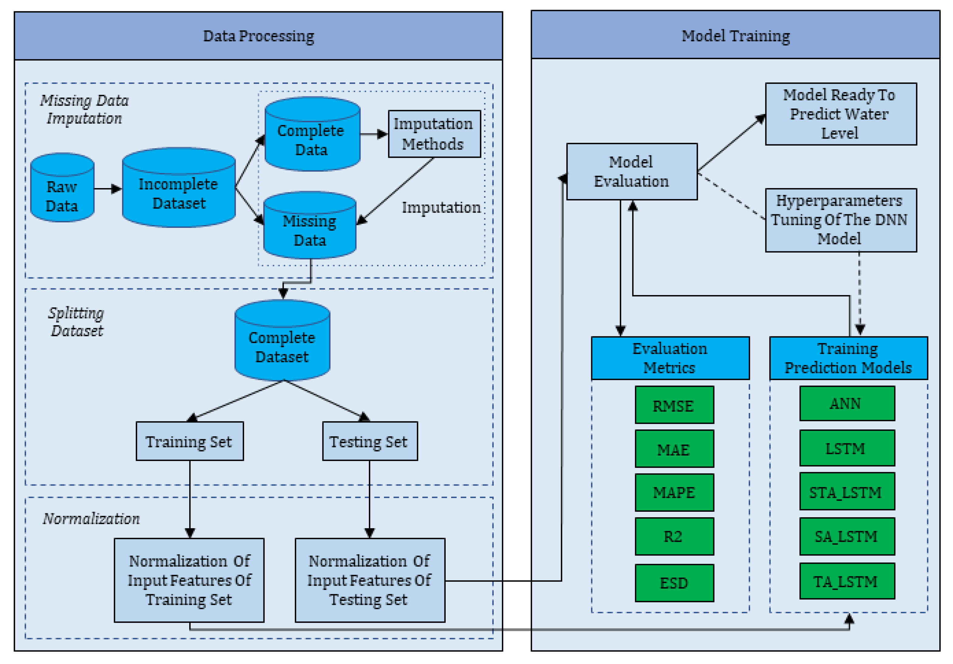
Figure 1 presents an overview of the methodological approach utilized in this study. First, we selected appropriate gauges for developing a multivariate water level prediction model. The acquired water level dataset, however, contains gaps. Thus, an imputation technique is applied to replace the missing data with some substitute value. The processed dataset is split into training and testing sets. The first 80% of the dataset is taken as the training set, and the remaining 20% is used to evaluate the performance of the model. Using the normalized training data, we established five neural network models: ANN, LSTM, spatial attention LSTM (SALSTM), temporal attention LSTM (TALSTM), and spatiotemporal attention LSTM (STALSTM). The performance of these models was assessed using various evaluation indices.
All neural network models had the same structures and were trained under the same hyperparameters, which helped to compare the models. Using the grid search technique, the optimum dimension of the hidden layer for the models was chosen to be 300. The Adam algorithm was chosen as the optimizer, and the mean square error (MSE) was used as the loss function for all the predictive models. The batch size was set at 600, with the epoch set at 100 and the learning rate at 0.1.
3.1. Study Area
In this study, water level forecasting was carried out in two major cities of Bangladesh: Dhaka and Sylhet [
7,
8,
9,
14,
16]. These two case study regions were selected as they are highly vulnerable to riverine flooding [
55,
56]. Besides, forecasting model structure and time series water level data are available for all the stations relative to other regions of the country.
Dhaka, the capital, is located in the central part of Bangladesh and at the confluence of three major rivers: the Brahmaputra, the Meghna, and the Ganges. The geographical location of the city makes it extremely susceptible to flooding [
9,
14].
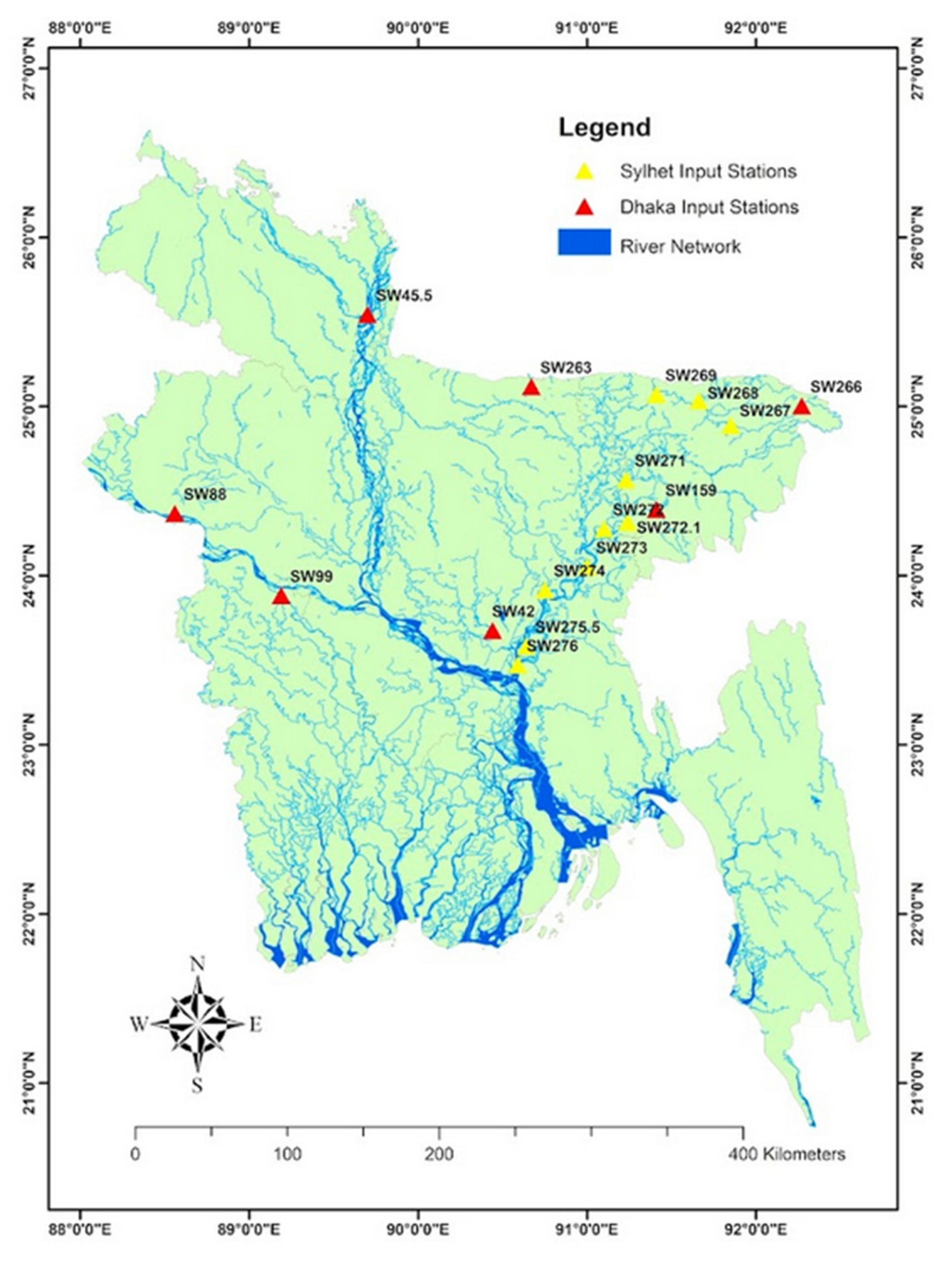
Sylhet, located in the northeastern part of Bangladesh, is characterized by the country’s longest river network (i.e., the Surma–Meghna River System) [
7,
8]. The geographical structure and the dense river network have made it extremely susceptible to flooding during the monsoon months when the rivers receive a heavy discharge from the upstream hilly regions. The locations of these stations are shown in
Figure 2.
3.2. Dataset
This study used daily water level data from May 1985 to October 2008 at the selected stations collected from the Bangladesh Water Development Board (BWDB) [
15]. For each of the two regions, several station data were considered independent variables to establish multivariate models. Since Bangladesh is a country filled with intricate networks of rivers, it is difficult to determine which river networks have a strong influence on Dhaka’s water level without having the necessary domain knowledge. However, a study by Liong, Lim, and Paudyal [
9] used stations near the borders of the country to forecast the water level of the Dhaka station as 90% of the annual water in all the major stations flows from outside the country. For this study, we selected the same stations to predict the water level of the Dhaka station.
For Sylhet, no such multivariate studies have been conducted from which we could select appropriate stations to utilize as input. Since the Sylhet station is one of the few stations that monitor the water level of Bangladesh’s largest river system, the Surma–Meghna Rivers, we took all the existing stations as independent features. Moreover, a dense network of hydrological features is recommended to be used in order to take the spatial and temporal variation of the stations into account [
39].
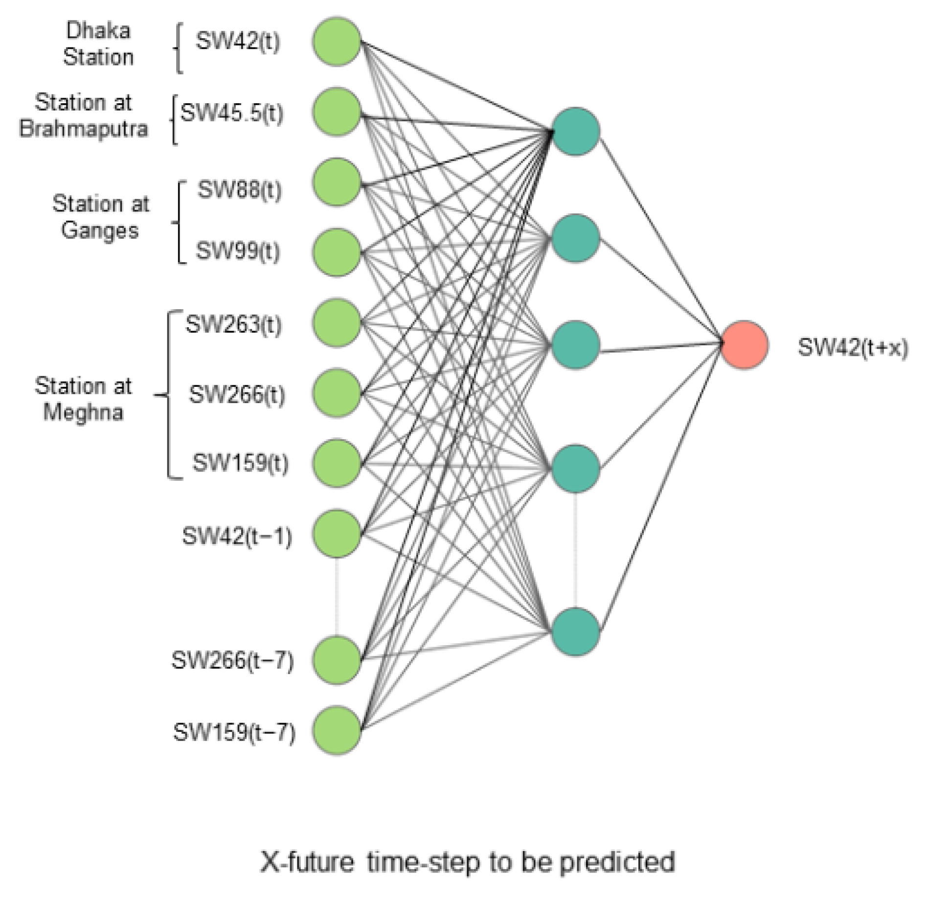
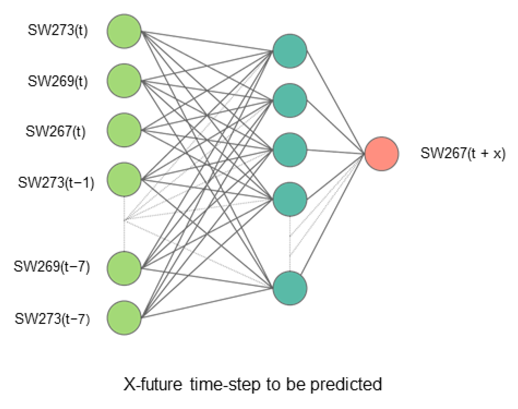
In this study, we analyzed the water levels of the Sylhet and Dhaka basins and predicted flood water levels at the main stations. Sylhet (SW267) and Dhaka (SW42) are the main stations of the basins, respectively. Floods at these two stations are forecasted using the water level data of all other stations. For both of these stations, the input feature for a period of 7 days was taken to make predictions up to 7 days into the future. For this study, we developed five neural network models. The input and output of the predictive models to forecast the stations of Dhaka and Sylhet are shown in
Table 1.
Correlation analysis was carried out to verify how correlated the input variables were with the output, estimating the Pearson correlation coefficients [
57]. Pearson correlation coefficients are used to measure the relationship between two sets of data.
Table 2 presents the interpretation of correlation values. The correlation coefficients of stations in Dhaka and Sylhet are given in
Table 3 and
Table 4, respectively.
The correlation coefficients for all the inputs to their corresponding output are greater than 0.5. It can be noted that the majority of the input stations chosen for the study are highly correlated to the output stations. To perform the multivariate time series forecasting, we chose 7 stations as our input features to forecast the water level of the Dhaka station. To forecast the water level in Sylhet, we chose 10 stations as independent variables.
3.3. Dataset Preprocessing
3.3.1. Imputation of Missing Data through Mice
Figure 3 and
Figure 4 provide a summary of the missing values of input features. The bar plot (left side) represents the percentage of missing data for each of the stations in the dataset. The level plot (right side) represents the combination of data—both missing and present. In the level plot, the available data are shown in blue color, and missing data in yellow color. The level plots are developed for a specific time frame, so the number of yellow/blue bars in the level plot will only count the data for a specific time. The highest proportion of missing data is found in stations SW268 and SW271, where more than 30% of data are missing.
The number of missing values is larger in stations around Sylhet than those located adjacent to Dhaka. Discarding missing data would significantly reduce the number of observations at each station, which may lead to bias and loss of critical information. Hence, we performed data imputations to address the data gap. Since water level data at different stations are missing randomly, we used the multiple imputation by chained equations (MICE) technique to impute the data gap [
58]. MICE is robust and one of the widely used approaches to overcome a large amount of missing data [
58]. It imputes missing data by assuming that the data missing are random in the series. It creates different sets of imputed datasets, which allows for using the best-imputed set. The data imputation process involves five steps:
Step 1: Perform simple imputation, such as mean imputation, on the dataset.
Step 2: Select the variable with the lowest missing data. Remove the imputed value of this variable.
Step 3: Use a regression model to predict the missing value of the selected variable by using other existing variables. The selected variable is considered to be the dependent variable, and the other variables are to be independent variables.
Step 4: Impute the missing value of the dependent variable using the regression model.
Step 5: Select the next variable with a missing value.
Step 6: Repeat steps 2 to 5 for all variables.
3.3.2. Min–Max Normalization
Since different stations had various magnitudes of water level, we performed min–max normalization on the input features using Equation (13). The dataset was first split into the train and test set, and then normalization was applied to prevent losing information of the training set.
3.4. Models Employed
3.4.1. Artificial Neural Network (ANN)
Artificial neural networks (ANNs) are mathematical function systems developed based on the inspiration of biological neurons. Instead of synapses in the human brain, an ANN model has artificial neurons, and instead of axons, it has weights. The model is typically constructed with various connections among nodes arranged in layers. It can have different numbers of layers. Two nodes from two layers are connected by an edge, and every edge has its weight. Each node in ANNs receives a signal, and then processes it and signals the node connected next to it. The “signal” or “response” from a neuron is a real number, and this response or signal is calculated by some linear or nonlinear function with the basic weighted sum approach. Neurons may have a threshold such that a signal is sent only if the aggregated signal crosses that threshold, which is controlled by functions called activation functions.
Figure 5 and
Figure 6 represent an ANN structure that will be used in this study to forecast the water level.
3.4.2. Long Short-Term Memory (LSTM)
The long short-term memory (LSTM) network [
38] is an artificial recurrent neural network (RNN) model that can remember the order in sequential data. The two major problems of the traditional RNN architecture are the vanishing gradient problem and its inability to retain information of long sequences. LSTM overcomes these issues with the help of its cell state and gates. The architecture of the LSTM model allows it to perform well in time series forecasting.
LSTM consists of three gates that control the flow of information. These three gates are input gate (it), output gate (ot), and most importantly, forget gate (ft). The hidden state of the LSTM network is the short-term memory, while the cell state is the long-term memory. Operations within LSTM cells help the model retain the information of sequential data. LSTM uses cells as the memory box for the model. The forget gate, shown in Equation (2), determines how much information from the previous timestamp needs to be forwarded to the current cell state:
where
represents the weight matrix that connects the input layer of its cell to the hidden layer. The input gate controls what extent of information is necessary to be added to the new cell state (
) In Equation (3), it is mathematically described that input gate takes in the previous hidden state (
) value and the input of the current time step (
) value.
In Equation (4), the output gate values are generated by passing the information of the current input and previous hidden state
through the sigmoid activation function. In Equation (5),
is produced based on the current input,
, and the previous hidden state. Then, taking the previous cell state,
,
is used in Equation (6) to produce the current cell state,
. Lastly in Equation (7), the output gate as well as the new cell state output helps to determine the new hidden state,
.
Due to the usage of the sigmoid function, the value of the gates remains between 0 and 1. The closer the value of the output of these gates gets to 0, the more it indicates that the information is not worth remembering. Similarly, a value closer to 1 increases the importance of the information. Moreover, the LSTM uses the hyperbolic tangent function to determine the current hidden state (), which helps increase and decrease the cell state.
3.4.3. Attention
All the input stations used for prediction may or may not influence the water level forecasting. However, it is known that the river networks that are closer to the output station or more deeply connected to the output station will have a greater influence [
9]. However, the nature of the water flow of the rivers in Bangladesh is complex to determine the actual river network, which might be having a greater influence. This influence may keep changing with time. As the river network system is affected by many geographical factors, it is difficult to identify which hydrological factors influence the most without having expert domain knowledge. Moreover, using irrelevant data for the prediction can lead to model inaccuracy. Hence, it is a challenge to make an accurate prediction as basic predictive models are unable to understand the importance of different features and how the importance of one feature can be more than the other.
Therefore, a deep learning model that uses an attention mechanism can overcome such a challenge. Attention has been widely used in sequence models to improve the accuracy of the prediction [
38,
39,
51]. Attention allows models to narrow down their focus on important features. Attention is a module that helps deep learning models to gain the ability to focus on crucial information from all the data available to it. The attention module has also proven to increase the accuracy of deep learning models.
Attention is of two types: hard and soft attention. Hard attention is useful when the model needs weight with a value of either 0 or 1. On the other hand, soft attention distributes the weights within the range of 0 to 1. Hence, compared with hard attention, soft attention provides more flexibility in assigning weights. For our study, we will be using soft attention.
From all the information presented to a model, the attention mechanism can help the model to focus on critical information. With spatial and temporal features of a time series dataset, we can use attention to find correlations among the different features changing over time and thus put more focus on the important features.
3.4.4. Spatial and Temporal Attentions
The spatial attention LSTM uses the spatial attention module to find out the correlation between independent feature and output. In this study, we are forecasting the water level of a certain station using the water level from its nearby stations. Water levels from different stations and locations are taken as input features to predict the water level of a particular station. However, not all the input features need to have a positive effect on the output feature. Giving excess weight to a feature that does not provide any contribution to the output variable will lead to inaccuracy. In the case of spatial data like this, it becomes difficult for the deep learning models to find out the correlation of different spatial data to the output. Therefore, implementing spatial attention to the base neural network will allow the model to understand the spatial correlation of the stations to the station that will be predicted.
To produce spatial attention, we used probabilistic activation sigmoid function as the function generates a value based on the input feature, and then the softmax is used to normalize the values. The production of attention weights is shown in Equation (9). Then, by element-wise product, shown in Equation (10), as
, the spatial attention is being implemented to the feature matrices in Equation (8):
where
n represents the total input features that will be processed in a single time step, while
k represents the different time steps. The element-wise product is also known as the Hadamard product, where identical matrices are being multiplied to produce another matrix of a similar dimension.
Temporal attention can be used to model the dynamic correlation between different time intervals in the target time series. Incorporating the spatial attention module and temporal attention module in an LSTM network can create a spatial-LSTM and temporal-LSTM, respectively [
38]. The temporal attention allows the model to focus on moments, which is most influential for the forecasting of the output for that time step. For example, in our study, we are taking the water levels of multiple water-level stations for 7 days to predict water levels in the next time step (i.e.,
n + 1 to
n + 7 time step). The temporal attention enables deep learning models to distribute weights of the independent variables based on time. In Equation (12), the temporal attention is generated after the weights are passed through ReLU and then through the softmax. In Equation (13), the temporal attention takes in the hidden layer states from Equation (11) to produce modified hidden weights with temporal attention incorporated within it.
denotes the matrix product.
3.4.5. Spatiotemporal Attention LSTM (STALSTM)
By implementing both the spatial and temporal attention to a neural network model, it will allow the model to narrow its focus on the spatiotemporal aspect at once.
One of the major benefits of the spatiotemporal attention LSTM model is that it can automatically select informative factors based on the inherent characteristics of the collected historical data. The STALSTM can identify key variables and moments important for forecasting and more suitable for multivariate time series data. With the implementation of both spatial and temporal attention, the neural network model is also able to identify the dynamic changing relationship of the independent variable to the dependent variable. Thus, a spatiotemporal attention-based model can overcome problems, faced by basic deep learning architecture.
The attention mechanism can find out key features that are responsible for the changes in the water level of the station to be forecasted. Thus, a model like the spatiotemporal attention neural network model can prove to be useful in such cases.
Implementing a spatial attention module and a temporal attention module in the LSTM can help the predictive deep learning model to figure out which of the input features is important for forecasting. The spatial module of the STALSTM will identify the complex relationship among the features and allow the model and would put more focus on those important features. For spatial attention, the feature vectors are passed through the sigmoid function to generate weights with respect to each feature. The higher is the importance of a feature, the more attention weight is generated for it.
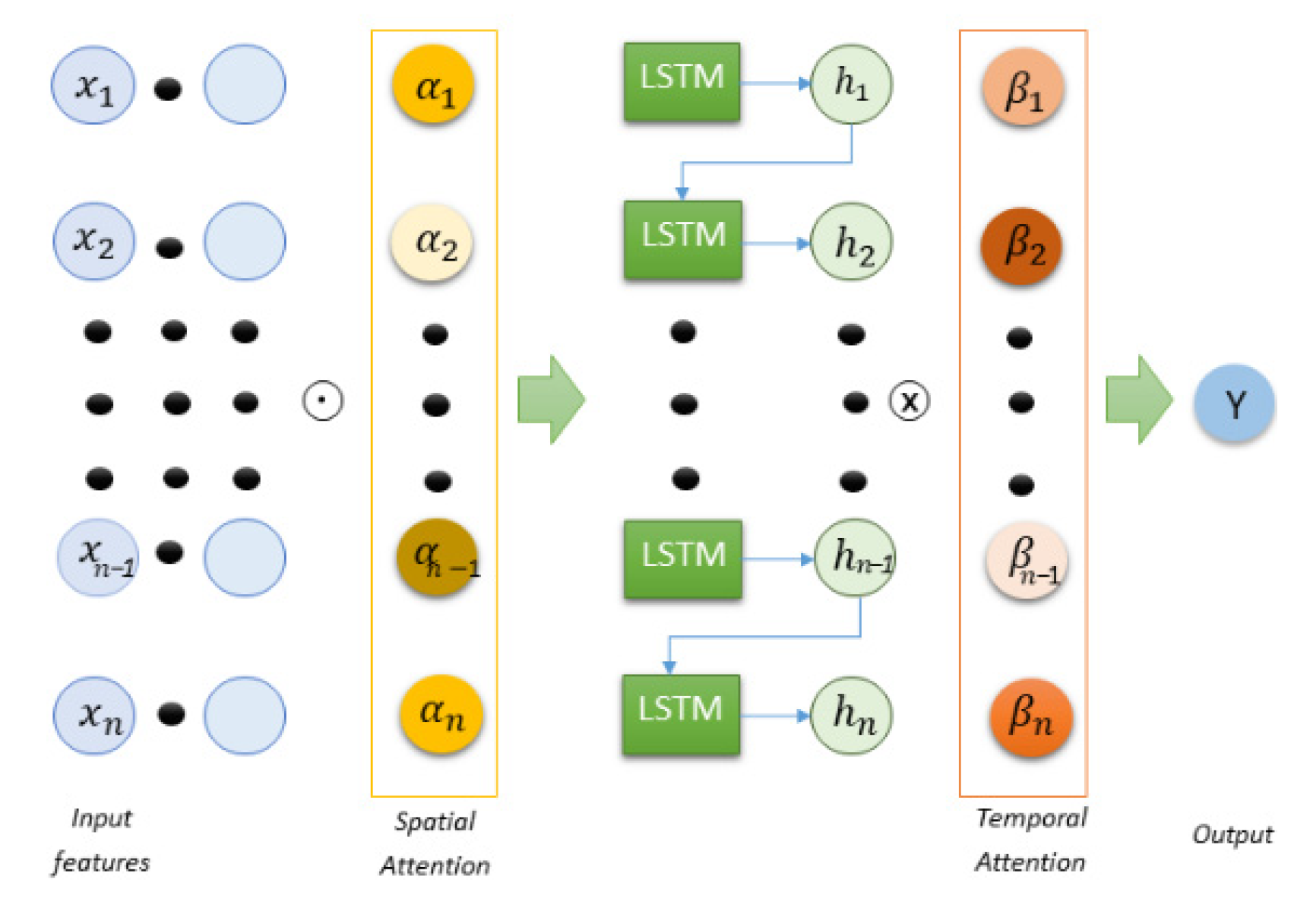
The structure of the spatiotemporal attention LSTM used in this study is shown in
Figure 7. This modified LSTM structure has been proven to increase the accuracy of LSTM models [
38,
39]. In
Figure 7, the input features represent the input stations that will be used by the model to forecast the water level of a station. After the element-wise operation of the input features and the spatial attention module, the data are then passed to the LSTM cells. The temporal attention would then be incorporated into the hidden layer states, as shown in Equation (11), to produce modified hidden weights with temporal attention incorporated within it. Thus, these attention modules allow the STALSTM to take spatial and temporal variation for making predictions.
3.4.6. Evaluation Criteria
To select the best-performing model, we selected six most commonly used evaluation metrics used in time-series analysis. The model, showing the best performance under most of the evaluation metrics, is selected as most efficient and accurate to forecast water levels.
For these evaluation metrics, represents actual value, represents predicted value, and represents the total number of test samples. The evaluation metrics used in the study are as follows:
RMSE is the root mean square error, which is one of the widely used metrics to analyze the accuracy of forecasting. The formula is shown in Equation (14).
MAE is the mean absolute error.
MAE helps us to understand how well the models are able to accurately predict and by what amount these values are deviating from the actual one. The formula is shown in Equation (15).
MAPE is the mean absolute percentage error. The formula is shown in Equation (16).
R2 is the coefficient of determination. It helps to analyze the performance of the model. A higher value of
R2 represents a better fit for the model. The formula is shown in Equation (17).
ESD is the error standard deviation. Here,
e represents error, and
represents the dispersion between the predicted and observed data. The formula is shown in Equation (18).
NSE is the Nash–Sutcliffe model efficiency coefficient. This statistical criterion is used to determine model performance. An NSE value greater than 0.75 represents good performance of the model [
59].
4. Results and Discussions
Table 5 shows the average performance of the models for forecasting water levels in main stations, located in Dhaka and Sylhet. From the evaluation metrics, it can be seen that the STALSTM model has the best forecasting results. Lower values of
RMSE and a higher value of
R2 indicate a higher level of prediction accuracy. The overall performance of the neural network is better for stations in Dhaka than Sylhet. This may reflect a greater number of missing data in the Sylhet stations. Any changes in the imputation method can influence the accuracy of predictions [
55]. Data cleaning methods may also impact the performance of the model. Overall, the STALSTM model outperformed other neural network models tested in the study. This is because the model inherits both spatial and temporal attention and utilizes a mechanism to make reliable predictions [
38]. The STALSTM model outperformed the basic LSTM model. This indicates that the attention mechanism has a positive effect on its performance [
49]. The error trend of all attention models is similar to the LSTM as it is used as the base. Among all the neural network models employed in the study, the performance of the ANN is least for both the Dhaka and Sylhet stations. Unlike the LSTM, the ANN lacks a memory cell, which is needed to retain long sequences of information to make predictions [
38,
39,
41].
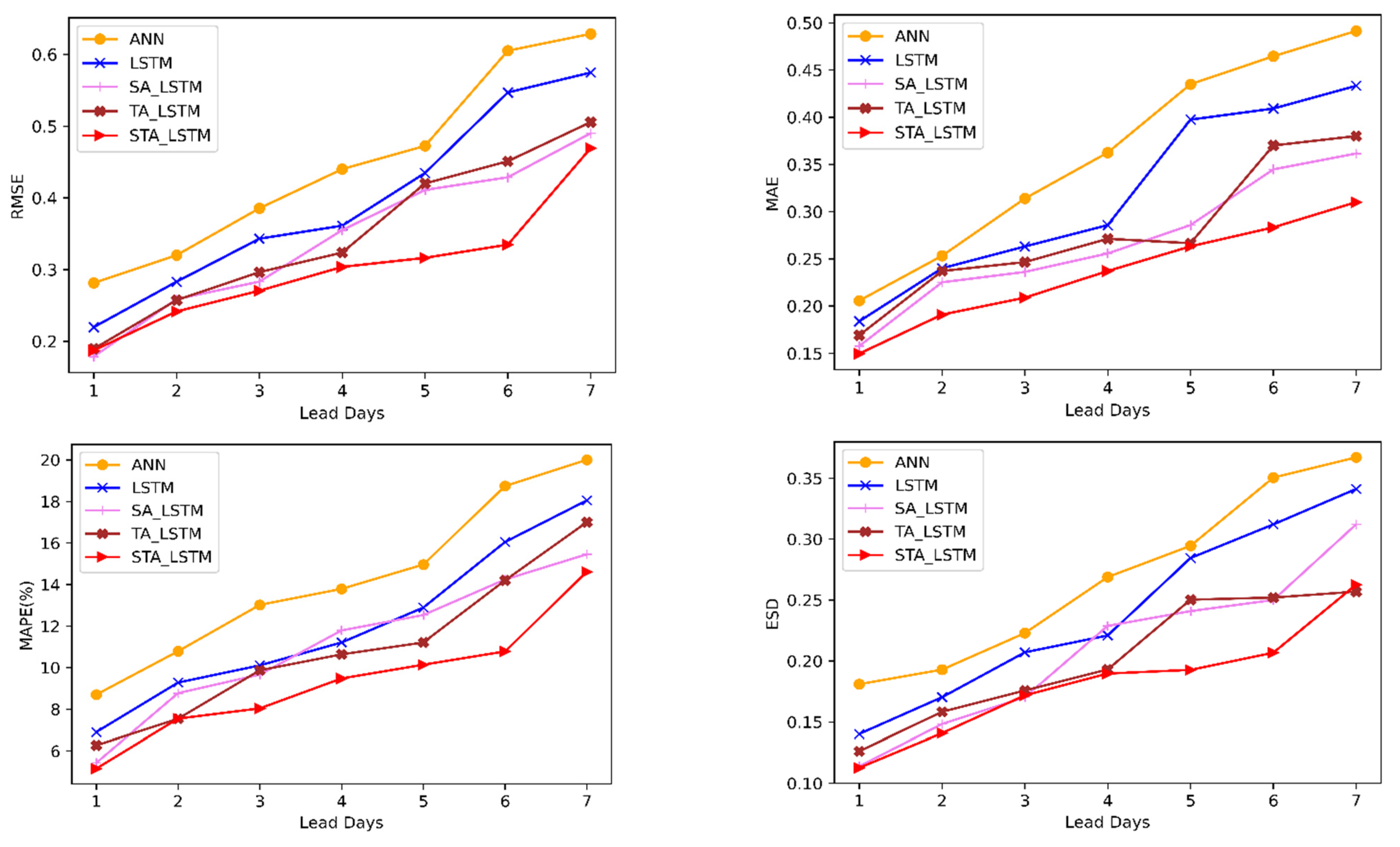
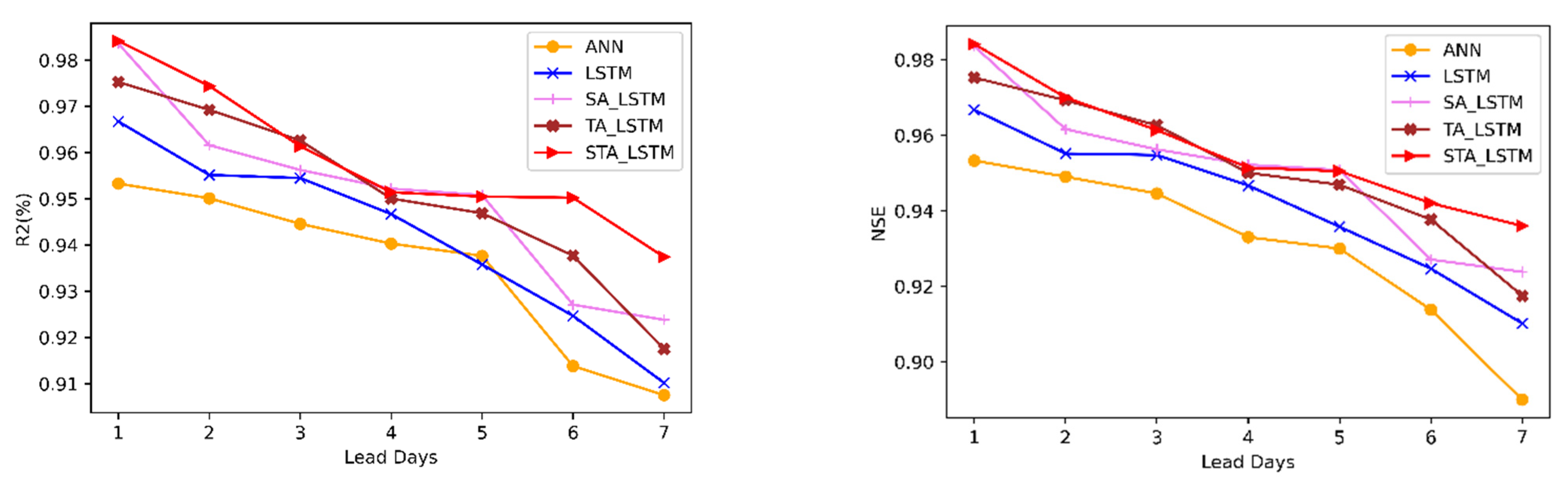
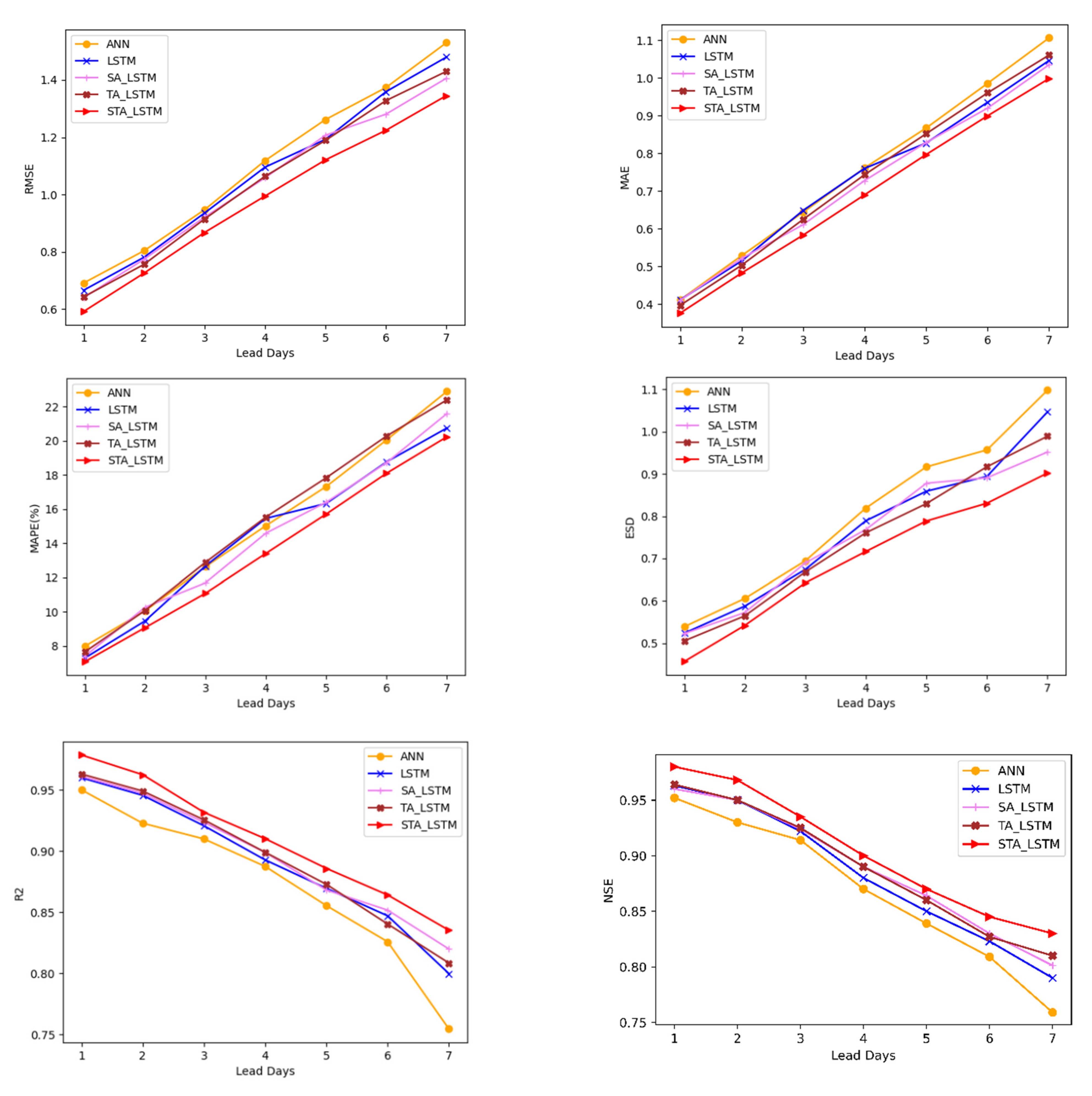
Figure 8 and
Figure 9 represent the performance of the predictive models on forecasting the Dhaka station and the Sylhet station for all different time steps for each of the evaluation metrics. For all the future forecasting, the STALSTM model shows the least
RMSE.
Figure 8 and
Figure 9 also show how the performance of the models changes with the lead day. As the number of days increases, the error for each model increases. There is a difference in the performance of the ANN and LSTM due to the difference in the model architecture.
Compared with other models, the incorporation of attention methods drastically improved the forecasting accuracy. The spatial attention module puts more weight on the appropriate input features for a certain time step prediction [
38,
39]. By providing adequate relevant features to the input, the STALSTM was able to outperform all other models. The lowest error achieved in this model suggests that it is successful in capturing the importance of variables in the prediction of the water level at a certain time step.
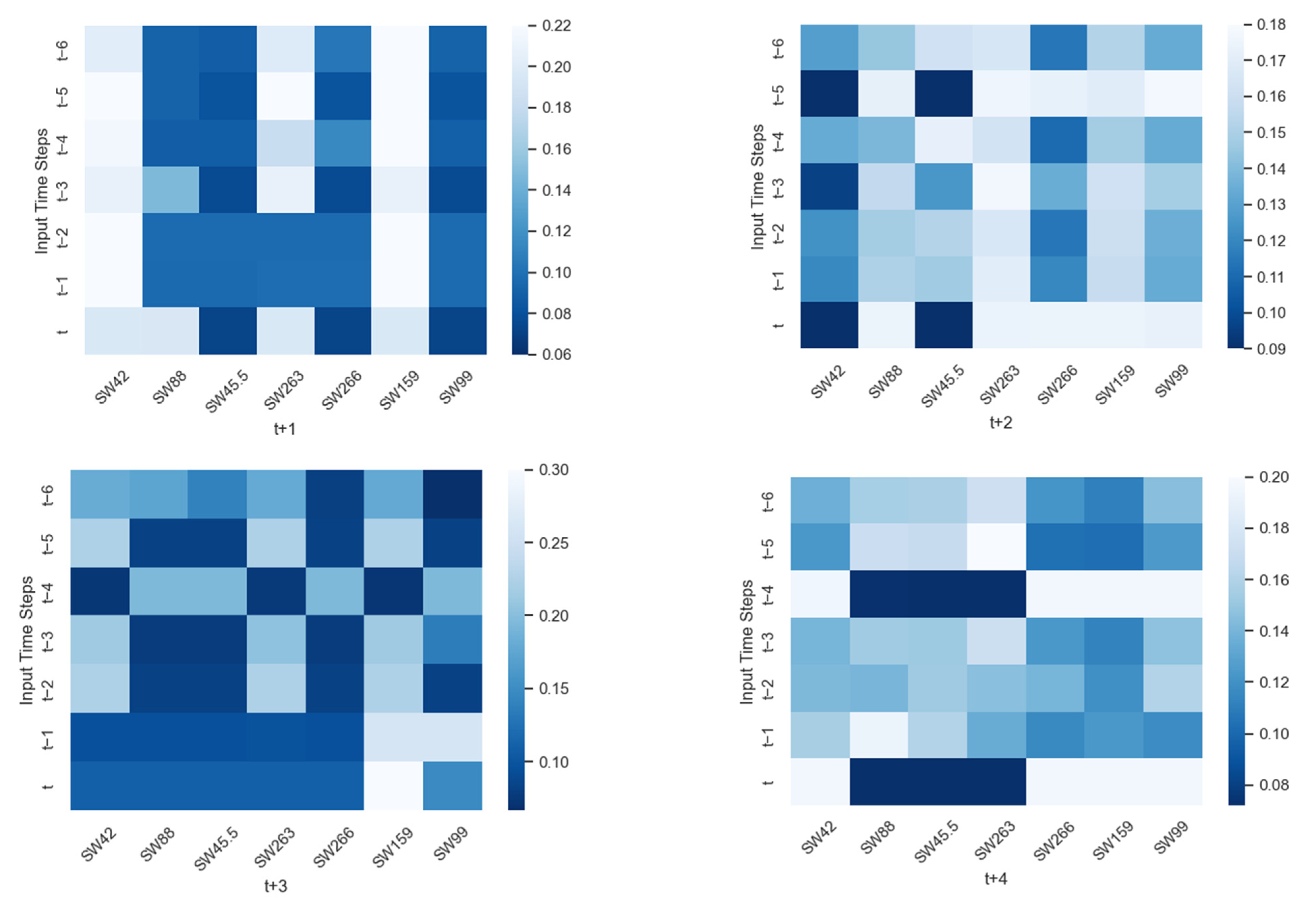
To assess the performance of the STALSTM, the attention weights are extracted and visualized.
Figure 10 illustrates weights of the STALSTM model used to predict the water level of the Dhaka stations. Light color represents low attention weights, and dark color denotes high attention weights. The bar presented on the right of the heat maps represents the attention weight values. Here, the attention weights are not only different for varying moments in time, but also different on input features. If the model is given an
n-previous time step to forecast one step ahead, the model is most likely to take values from the moment it fits. For forecasting of the Dhaka station at a one-time step ahead, the SW159 station with
t − 2 has been assigned with more weights compared with other stations. This is because, at a certain time step, the attention mechanism increases the weights of input information, which are useful for that time step [
38].
It is worth noting that the further into the future the model is used to make a prediction, the more the model focuses its attention on the values that are nearby to the present time,
t. The attention moves its focus towards more recent water level values of the input. When predicting water levels 7 days into the future, we can see how the attention module focuses by putting more weight on the values in the current day. Hence, attention weights for
t + 7 are more for the more recent historical moment of the Dhaka station. Therefore, it can be observed how the distribution of spatial and temporal attention modules can enable the LSTM architecture to capture the complex relationship to perform accurate flood forecasting [
54,
60].
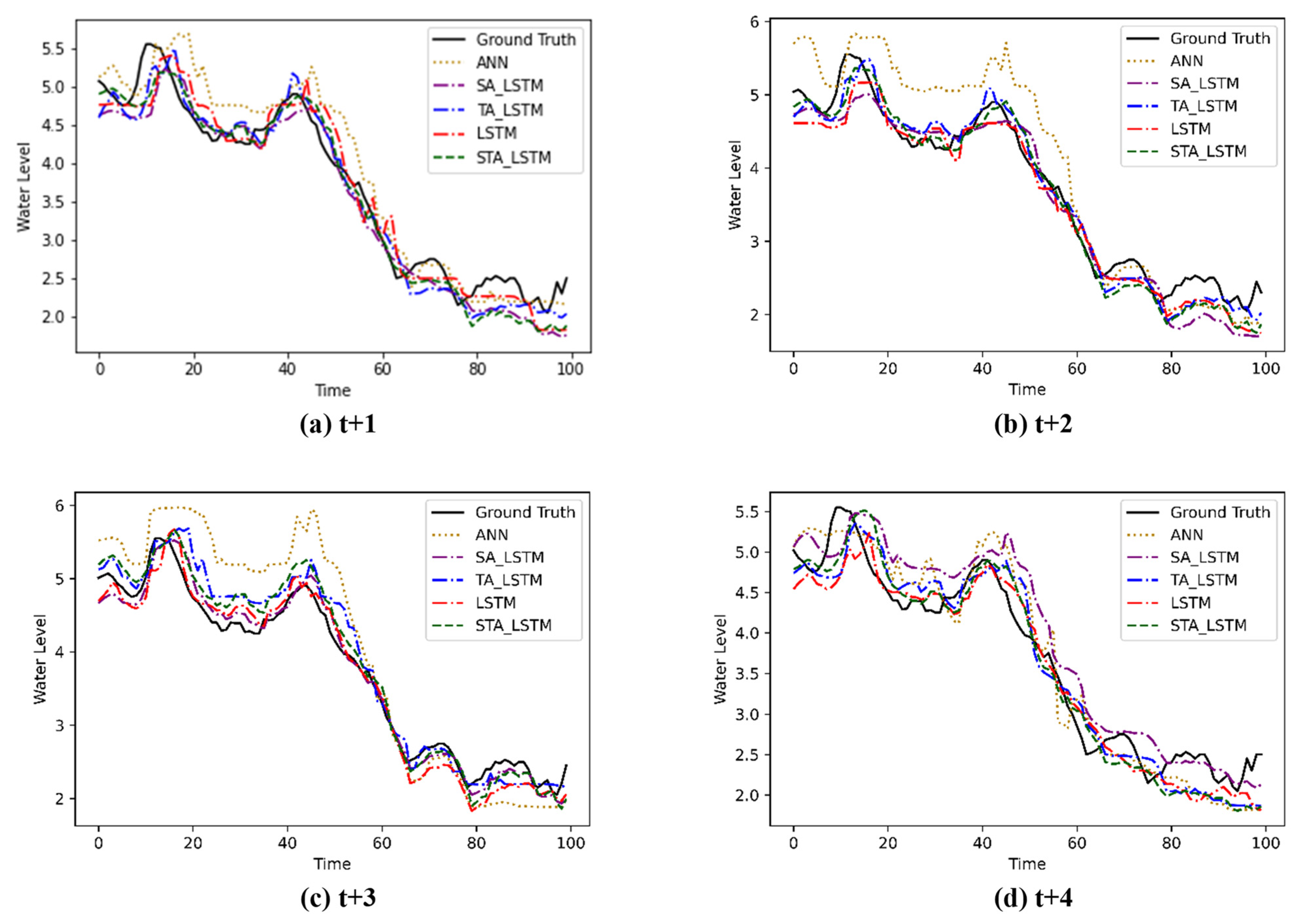
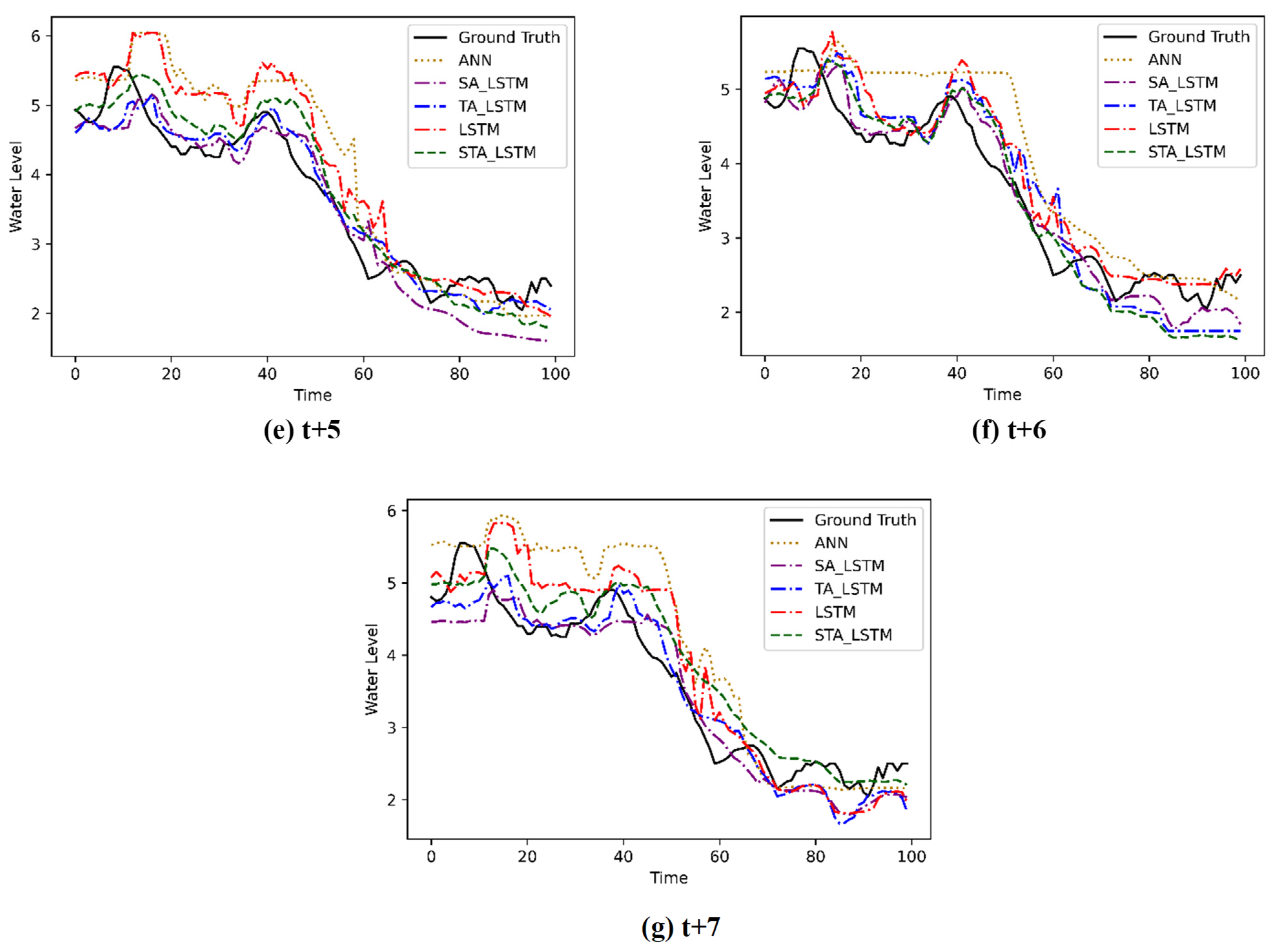
Figure 11 represents a subsection of the predictive models forecasting on the testing set for the Dhaka station, where prediction can be compared with ground truth information. Here, increasing the lead day makes the prediction performed by the model more uncertain. For
t + 1, the prediction model is close to the actual water level. However, with an increasing lead time, the predictions become more far off than the actual value. Among all the models used in this study, the STALSTM shows the most stable performance. The prediction of the ANN model fluctuated more heavily compared with other models. The fluctuations are observed near the peaks due to sudden changes in water level.
The results, obtained from the study, illustrate that when using multivariate time series to make multistep ahead prediction, the LSTM or its variants can perform better than the ANN model due to the advantage of having the ability to retain a long sequence of information. The performance of the models can be ranked as follows:


 ,
, 


