
A Hybrid Model for Water Quality Prediction Based on an Artificial Neural Network, Wavelet Transform, and Long Short-Term Memory


1
College of Economics and Management, Shanghai Ocean University, Shanghai 201306, China
2
College of Information, Shanghai Ocean University, Shanghai 201306, China
*
Author to whom correspondence should be addressed.
Water 2022, 14(4), 610; https://doi.org/10.3390/w14040610
Submission received: 7 December 2021
/
Revised: 10 February 2022
/
Accepted: 10 February 2022
/
Published: 17 February 2022
(This article belongs to the Special Issue Decision Support Tools for Water Quality Management)
Abstract
:Clean water is an indispensable essential resource on which humans and other living beings depend. Therefore, the establishment of a water quality prediction model to predict future water quality conditions has a significant social and economic value. In this study, a model based on an artificial neural network (ANN), discrete wavelet transform (DWT), and long short-term memory (LSTM) was constructed to predict the water quality of the Jinjiang River. Firstly, a multi-layer perceptron neural network was used to process the missing values based on the time series in the water quality dataset used in this research. Secondly, the Daubechies 5 (Db5) wavelet was used to divide the water quality data into low-frequency signals and high-frequency signals. Then, the signals were used as the input of LSTM, and LSTM was used for training, testing, and prediction. Finally, the prediction results were compared with the nonlinear auto regression (NAR) neural network model, the ANN-LSTM model, the ARIMA model, multi-layer perceptron neural networks, the LSTM model, and the CNN-LSTM model. The outcome indicated that the ANN-WT-LSTM model proposed in this study performed better than previous models in many evaluation indices. Therefore, the research methods of this study can provide technical support and practical reference for water quality monitoring and the management of the Jinjiang River and other basins.
1. Introduction
Water is one of the most essential natural resources on which all life depends. However, various economic activities have an indispensable impact on the environment through different pathways [1]. Take China as an example: in recent years, along with high-speed economic development and urbanization, China’s limited freshwater resources have been drastically reduced and, at the same time, increasing water pollution poses a serious threat to human survival and security and has become a significant obstacle to human health and sustainable socio-economic development. From the perspective of China’s actual national conditions, water resources are relatively scarce. In addition, as China is undergoing a period of rapid socio-economic development, the demand for water resources is accelerating. Although China has 2.8 trillion water resources [2], which seems to be very rich, the per capita share of water resources is only 2400 cubic meters due to its large population [3], and account for less than one-quarter of the world’s total per capita water resources. In addition, the discharge of industrial wastewater and domestic sewage into water bodies without treatment has led to the severe pollution of various water bodies, including rivers and lakes, thus seriously damaging the ecological environment, biodiversity, and the ecological and service functions of water bodies [4]. According to previous studies, only a small number of rivers worldwide are not affected by water pollution [5]. At present, the pollution and eutrophication of rivers in China are severe. According to the 2019 statistics from China’s State Environmental Protection Administration, the seven major water systems in China in descending order of pollution level are listed as follows: the Liaohe River basin, the Haihe River basin, the Huaihe River basin, the Yellow River basin, the Songhua River basin, the Pearl River basin, and the Yangtze River basin, with more than 70% of the Liaohe, Haihe, Huaihe, and Yellow River basins being polluted. Huang et al. [6] conducted an analysis of water quality data from 2424 water quality observation stations in China from 2003–2018 and concluded that the quality of river water in China showed significant spatial differences, with 17.2% of sampling sites in eastern China showing poor water quality during the period of 2016–2018, compared to 4.6% in the western region. Moreover, 24.4% of the sampling sites in coastal areas (buffer zone of 20 km from the coastline) showed poor water quality. Although the Chinese government has invested a great deal of money into the treatment and management of polluted water bodies, the pollution proportion of water resources is still quite impressive, which has brought severe economic and social costs to China’s water environment remediation [7]. Water quality prediction is a necessary tool for water environment planning, management, and control; an important element of water pollution research; and a fundamental part of water environmental protection and management. Thus, it is vital to find a reasonable and effective water quality prediction method. At the same time, predicting future water quality is a prerequisite for preventing rapid changes in water quality and proposing countermeasures. Therefore, the accurate prediction of water quality changes can not only effectively ensure the safety of people’s drinking water, but can also have a positive impact on guiding fishery production and protecting biodiversity.
Research into water quality prediction dates back to the 1920s. Streeter and Phelps developed a coupled model based on biochemical oxygen demand and dissolved oxygen when they studied pollution sources in the Ohio River. They proposed a one-dimensional steady-state oxygen balance water quality model (the S-P model). Since then, many scholars have supplemented and revised their theories [8,9,10]. At present, the research methods of water quality prediction are mainly divided into two categories: one is to use theoretical mathematical model and physical model to predict the development trend of water quality mechanism [11], the other is a non-mechanistic prediction method that builds mathematical statistical prediction models based on historical data. The mechanistic prediction method analyses the physical, chemical, and biological changes of each factor in the water resource cycle; establishes a mathematical model reflecting the relationship between the substances; and solves the corresponding mathematical equations to predict the trend of water quality changes. For example, Zhang et al. incorporated the operation rules of dams or sluices into the reservoir regulation module, used an improved SWAT model to simulate the water quantity and quality in the Huaihe River basin, and compared the results with those of the original SWAT model. The results showed that the improved SWAT model was more accurate in simulating the water quantity and quality in the Huaihe River basin [12]. Peng et al. used the Environmental Fluid Dynamics Code (EFDC) model coupled with a geographic information system (GIS) model to simulate the water quality of the lower Charles River, and the results showed that the accuracy of the model was improved compared with the original EFDC model [13]. The mechanistic models of river water quality tend to provide a more comprehensive description of water quality changes, as they consider the effects of physical, chemical, and biological processes on the spatial and temporal transport and transformation patterns of pollutants in river waters; however, at the same time, most of these models are complex and require a great deal of basic information and data (numerical model uses a large amount of water quality data as the basis for calculation), and it is difficult to obtain a continuous distribution of water quality in space and time. This has greatly limited the application of these models [14]. In addition, the mechanics of many water environment systems are not fully understood by scholars; hence, it is difficult to describe them accurately using exclusively mechanistic modelling. In contrast, non-mechanical water quality modelling is a black-box approach to a particular water quality system, which is modelled by mathematical statistics or other mathematical methods to make predictions about water quality. Commonly used non-mechanical water quality simulation prediction methods include regression models, probability statistical models, grey prediction models, time series models, etc.
In recent years, neural networks and other machine learning algorithms have been applied by many researchers in the field of water quality prediction and have achieved good prediction results. The SOTA table of the progress of research based on water quality prediction is shown in Table 1 (distinguishing between mechanistic and non-mechanistic models).
Archana et al. used the depth belief network in unsupervised learning to study the PH, dissolved oxygen, turbidity, and other water quality parameters of the Chaskaman reservoir for prediction and analysis [31]. The results show that this method performs better than the classical method for prediction. Wang et al. introduced the Holt–Winters seasonal model based on the ARIMA model and predicted the total phosphorus and total nitrogen in the reservoir. The results showed that the model had a prediction accuracy of 97.5% and had many advantages, such as fast learning speed [32]. Mohamed et al. analyzed the irrigation water quality index in Egypt by means of an integrated evaluation method and an artificial neural network model. In addition, the ARIMA model was developed to predict IWQI in Bahr El-Baqar drain, Egypt [33]. Shi et al. proposed a combination of the wavelet artificial neural network (WANN) model and the high-frequency alternative measurement of water quality anomaly detection and early warning method [34]. Li et al. proposed an EEMD-SVR water quality prediction model to predict the water quality of Jialing River in China. The model first decomposes water quality indicators, such as DO, into each IMF component by the EEMD algorithm, and then builds the SVR model based on each IMF component. The results showed that the hybrid model outperformed the standard SVR model and BPNN model in a variety of evaluation indicators [35]. Ewaid et al. established a multiple linear regression model according to the specified weight and predicted the water quality of the Euphrates River [36]. Xu combined wavelet transform and BPNN to establish a short-term wavelet neural network water quality prediction model and used the model to predict the water quality of intensive freshwater pearl culture ponds in Duchang County, Jiangxi Province, China. The results showed that the RMSE of the model was 3.822 in DO metrics, which was much lower than that of the BPNN and ELman models, showing desirable performance [37]. Qin et al. developed a PSO-WSVR model and used a particle swarm algorithm to optimize the parameters of the weighted support vector regression machine to predict water quality in Yixing, China. The results showed that the model reduced RMSE, MAE, MAPE, and MSE by 46.74%, 17.86%, 43.62%, and 67.84%, respectively, compared with the standard SVR model [38]. Tizro et al. used the ARIMA model to study nine water quality parameters of Hor Rood River [39]. Faruk established an ARIMA-ANN model with 108 months of water quality data from the Büyük Menderes River in Turkey from 1996–2004. The model consisted of two parts: firstly, the ARIMA model was used to model the linear part of the dataset, and then the artificial neural network was used to model the nonlinear part of the water quality series based on the fact that the ARIMA model could not solve the nonlinear part of the water quality series well. The results showed that the correlation coefficients between the predicted values of the hybrid model and the observed data for boron, dissolved oxygen, and water temperature were 0.902, 0.893, and 0.909, respectively [40]. Zhang et al. developed an ARIMA-RBFNN model to predict the total nitrogen (TN) and total phosphorus (TP) of Chagan Lake. The results showed that the RMSE values of this hybrid model were 0.139 and 0.036 for TN and TP indicators, respectively, which were improved compared to the ARIMA and RBFNN models [41]. Than et al. developed the LSTM-MA model, classified the water quality of Dongnai River from 2012 to 2019, predicted the water quality in the next two years, and proved that the LSTM-MA hybrid model has a quicker training time and more precise prediction than ARIMA, NAR, NAR-MA, and LSTM models [42]. Jian et al. first used an improved grey correlation (IGRA) to extract the features of water quality information and subsequently used LSTM to predict the water quality of Taihu Lake and Victoria Harbor; the results showed that the RMSE values of the model were 0.07 and 0.067, which were lower than those of the BPNN and ARIMA models, showing good performance [43]. Hameed et al. used an RBF neural network (RBFNN) and BPNN model to forecast and compare the water quality in Malaysia, respectively. The results showed that the RMSE of BPNN was 0.867 and the RMSE of RBFNN was 0.0194, and the RBF neural network outperformed the BP neural network model in terms of prediction accuracy [44].
In summary, although scholars have proposed a large number of research methods in the field of water quality prediction, the prediction results of traditional statistical models are not satisfactory for time series with large fluctuations and long-term trends. For example, the regression analysis model is relatively simple, but its requirements for statistical data are high, demanding a large sample and data with a good distribution pattern; the time series model has a relatively sound theoretical basis, but its prediction accuracy is poor; the grey prediction model is suitable for the case of small and discontinuous historical data, but the model is susceptible to the influence of unstable data, resulting in a large prediction error; the support vector machine is suitable for small samples, but it is more sensitive to the choice of parameters and kernel functions. In addition, traditional single deep learning models, such as back Propagation neural network (BPNN) and RBFNN, lack the memory ability for historical information. Moreover, most of the missing data filling methods cannot effectively handle the time-series information in the dataset, resulting in large errors in the estimation of missing values. Therefore, this study attempts to use an artificial neural network to fill in the missing information of water quality, comprehensively apply wavelet transform and the LSTM model to the field of water quality prediction, and compare the prediction results with ANN-LSTM, ARIMA, NARNN, CNN-LSTM, and DWT-CNN-LSTM models so as to prove the effectiveness of the proposed model.
This study is divided into the following parts: Section 2 introduces the artificial neural network model, wavelet transform, long-short term memory network model, and error evaluation index; Section 3 takes the Jinjiang River Basin as the research object, constructs the ANN-WT-LSTM model for water quality prediction, and compares the prediction results with the NAR neural network model, ANN-LSTM model, and ARIMA model; and the conclusion and research prospects are presented in Section 5.
2. Materials and Methods
2.1. Study Area Description and Dataset Analysis
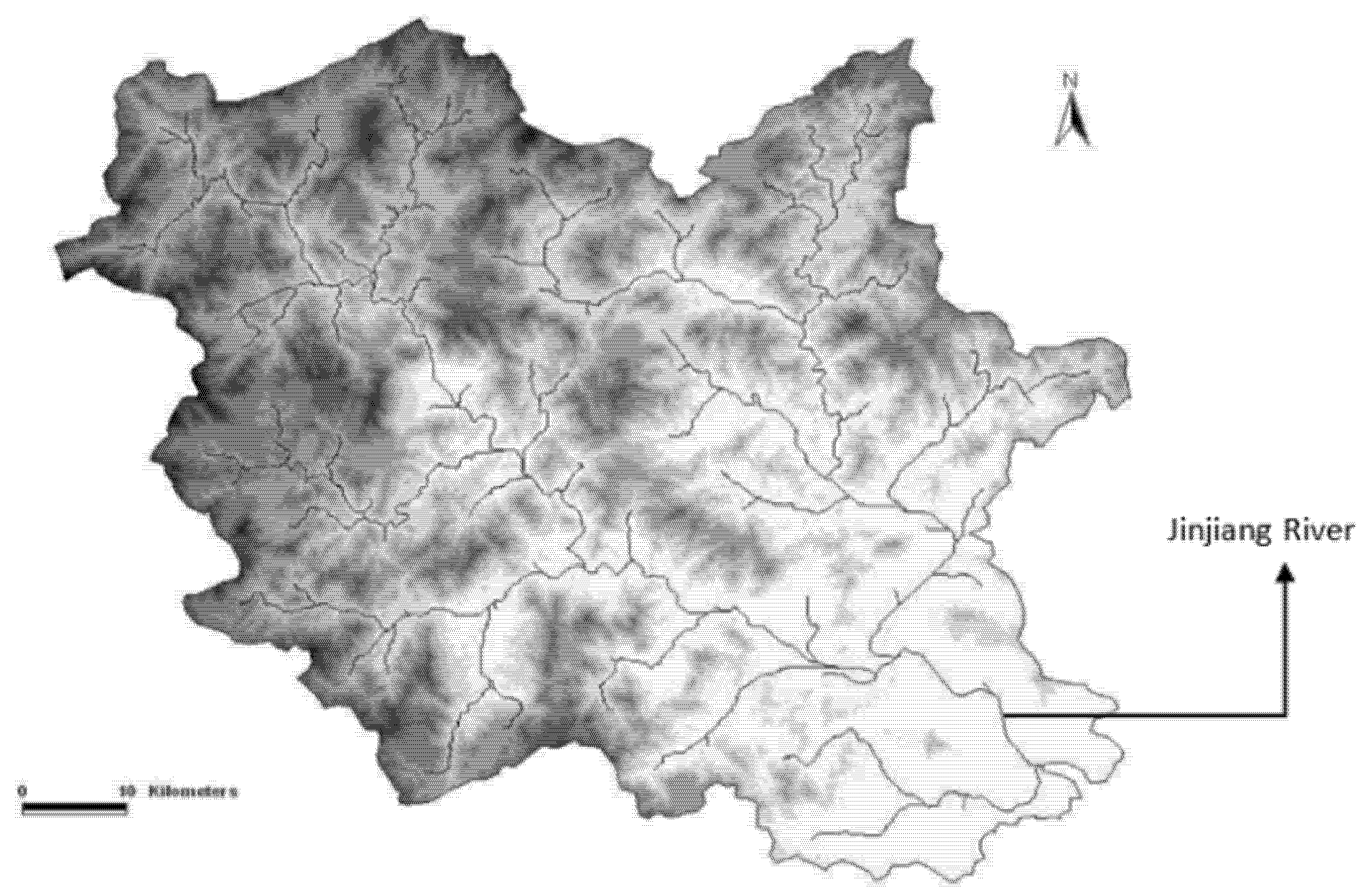
The Jinjiang River is 182 km long, with a watershed area of 5629 square kilometers, an average slope of 0.19%, and an average annual runoff of 5.13 billion cubic meters. It is the largest river in Quanzhou and the third largest river in Fujian Province. The following Figure 1 shows the geographical location of the Jinjiang River.
The Jinjiang River is divided into two tributaries, the east stream and the west stream, and the source of the Jinjiang River is the west stream, which is 153 km long with a watershed area of 3101 square kilometers and an average annual runoff of 3.65 billion cubic meters. The east stream of the Jinjiang River originates at the southern foot of Xueshan Mountain in Jindou, Yongchun. The river is 120 km long, with a watershed area of 1917 square kilometers and an average annual runoff of 1.4 billion cubic meters. Quanzhou City, through which the Jinjiang River flows downstream, is one of the most economically developed regions in Fujian Province. Quanzhou, located in the southeastern part of Fujian Province, is one of the three central cities in Fujian Province, and its total economic output has remained the first in Fujian Province for 22 consecutive years. In 2020, the city’s population was over 7 million, ranking first in the province in terms of population size. As the Jinjiang River basin covers 53.8% of Quanzhou’s land area, water resources are very important for the city’s sustainable development. At the same time, there has been a serious pollution problem in the Jinjiang River basin [45,46]. The traditional industrial development model has caused great damage to local sustainable development, the pressure on the water environment is increasing, pollution from some enterprises is rebounding, the construction of environmental protection infrastructure is lagging behind, and the proportion of domestic pollution sources is increasing day by day. Therefore, the accurate prediction of water quality in the Jinjiang River basin will provide crucial decision data support for future pollution control programs.
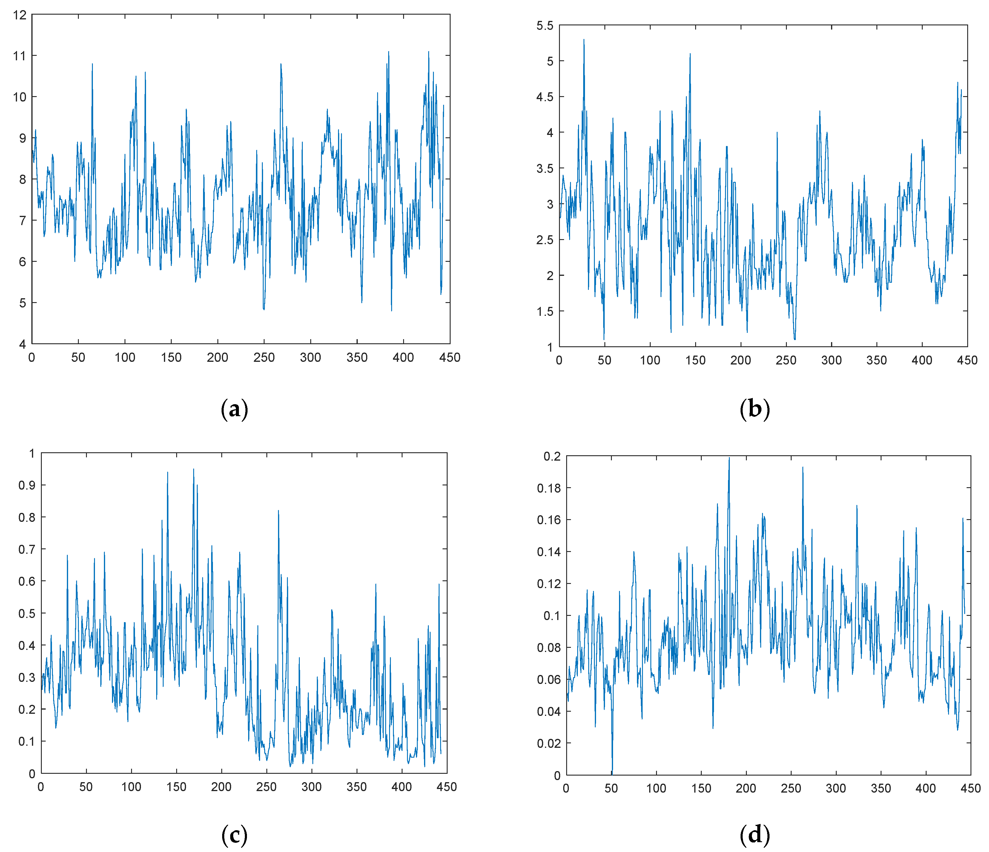
The dataset used in this study was selected from the weekly report of automatic water quality monitoring at the Shilong section of Jinjiang River basin. Among the many water quality evaluation indexes, we selected dissolved oxygen (DO), permanganate index (CODMn), ammonia nitrogen (NH3-N), and TP (total phosphorus), which are the four most representative indexes of the research object. The time of data collection was from 7 January 2013 to 21 June 2021. The data update cycle occurred once a week, with a total of 443 groups of data. We used the first 421 groups of data as the training set and the last 22 groups as the test set. The images of the dataset are shown in Figure 2.
Next, the dataset was analyzed and the missing values were found. The analysis results are shown in Table 2.
Then, we used Pearson’s correlation coefficient to analyze the correlation of each dataset. The results are shown in the Table 3. From the above correlation analysis table, it can be seen that the DO dataset was negatively correlated with the CODMn, TP, and NH3-N datasets; the CODMn dataset showed a weak positive correlation with the TP and a significant positive correlation with the NH3-N dataset; and the TP dataset showed a significant positive correlation with the NH3-N dataset.
2.2. The Framework of the Proposed Model
The single neural network model is susceptible to fluctuations in the water quality time series during training, which affects the prediction accuracy. Therefore, this study introduced the signal time and frequency decomposition method for water quality data preprocessing and built a hybrid prediction model based on “decomposition- prediction- reconstruction” to improve the overall prediction accuracy. The hybrid model is made up of five components:
- Data preprocessing: firstly make a descriptive analysis of the collected water quality data, find the missing value, estimate the missing value by artificial neural network, and then normalize it to eliminate the influence of dimension.
- Discrete wavelet transform: The db5 wavelet technique is used to decompose the water quality time series datasets.
- Model training, detection: Split the high-frequency and low-frequency signals of each dataset obtained from the db5 wavelet decomposition into a training set and a test set according to a fixed ratio. In this study, we set the first 421 sets of each dataset as the training set and the last 22 sets as the test set. Subsequently, we used LSTM to train each training set and adjust the relevant parameters of LSTM, such as learning rate and the maximum number of iterations.
- The predictions obtained from the decomposed test set of each sub-series are superimposed to obtain the final prediction results.
- Model evaluation: This study used four indicators—MSE, RMSE, MAE and MAPE—to evaluate the model’s performance.
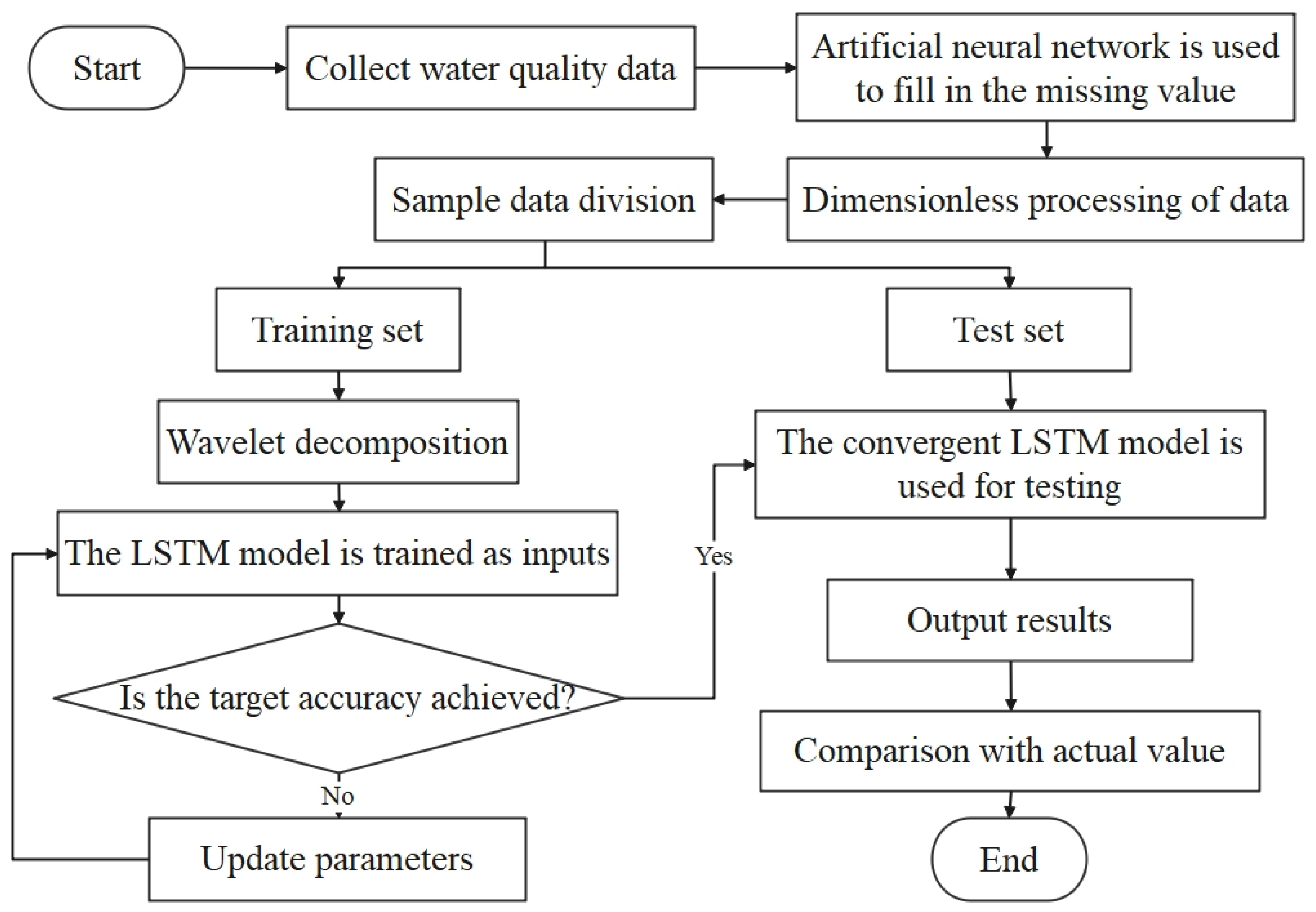
The whole algorithm flow chart is shown in Figure 3.
2.3. Data Normalization
Data normalization is a fundamental task for mining data in machine learning. In practical research, different methods and evaluation metrics often have different scales and units, which will produce diverse data analysis results. In order to reduce the relative relationship between quantities and to eliminate the influence of the dimension between indicators, the data must be normalized in order to achieve comparability between data indicators and to achieve the expectation of data optimization. The original data are normalized such that the indicators are in the same order of magnitude, which is convenient for comprehensive comparison and evaluation. Commonly used normalization methods include min-max normalization [47] and Z-score normalization [48]. Minimum-maximum normalization, also known as outlier normalization, is a linear transformation of the original data such that the resulting values map to between 0 and 1. There are also some other data normalization methods, such as the Z-score standardization method. However, the Z-score application also has risks. Firstly, the estimation of the Z-score requires the overall mean and variance, but this value is difficult to obtain in real analysis and mining. In most cases, it is replaced by the sample mean and standard deviation. Secondly, Z-score has certain requirements for data distribution, and normal distribution is the most conducive to Z-score calculation. Therefore, we chose the min-max normalization method. It is more suitable for use on data with relatively concentrated values. The transformation function of the min-max normalization used in this study is as follows:
where is the maximum value of the sample data and is the minimum value of the sample data.
2.4. Artificial Neural Network (ANN)
During the collection of time-series data, the loss of single or multiple attributes of some data in the final dataset or the loss of single or multiple records will be caused by acquisition, storage, and human error. These data are called missing data. The lack or incompleteness of data brings many difficulties to data mining, which will lead to the deviation of the analysis results and mislead users’ decisions, resulting in adverse consequences. Therefore, filling the missing data completely under certain conditions is of great significance for macro data mining in big data scenarios. Nowadays, there are several ways to deal with missing data, such as the deletion method [49,50], missing value filling method based on a statistical model [51], or the method based on parameter estimation. This method first judges the missing mechanism of the missing value and then establishes a specific model to estimate the missing value. This method is widely used because it is more flexible in application and can be applied to datasets with a large number of missing values [52]. Common methods include the expectation maximization method, multiple filling method [53,54,55,56,57], maximum likelihood estimation method, etc. Austin et al. used multiple interpolations to estimate missing values in clinical medicine [58]. Chang et al. developed a distributed multiple filling method with communication efficiency to estimate the missing data in distributed health data networks (DHDNs) [59].
In summary, research on interpolation methods for missing values of time series has received increasing attention from scholars in various fields, and although some scholars have considered the correlation characteristics of time series, most of these studies have not quantified the correlation between the observed quantities. Although some scholars consider the correlation characteristics of time series, most of the studies are still based on traditional interpolation or regression analysis methods. Moreover, some traditional models, such as piecewise linear interpolation [60], cannot estimate the missing value well [61,62]. Therefore, with the development of machine learning, researchers can gradually apply various machine learning algorithms to the field of missing value filling, which can to some extent solve the problem of non-linearity that cannot be handled by traditional methods. Machine learning methods for missing value estimation include the KNN method [63], artificial neural network, etc.
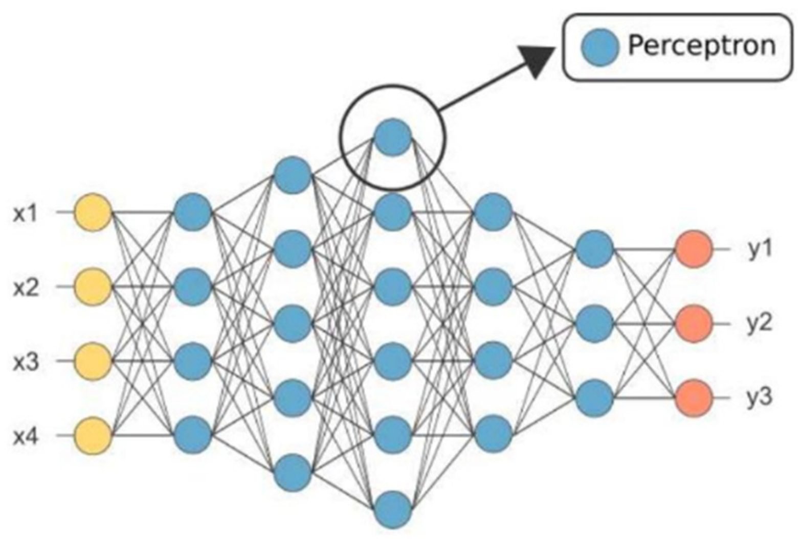
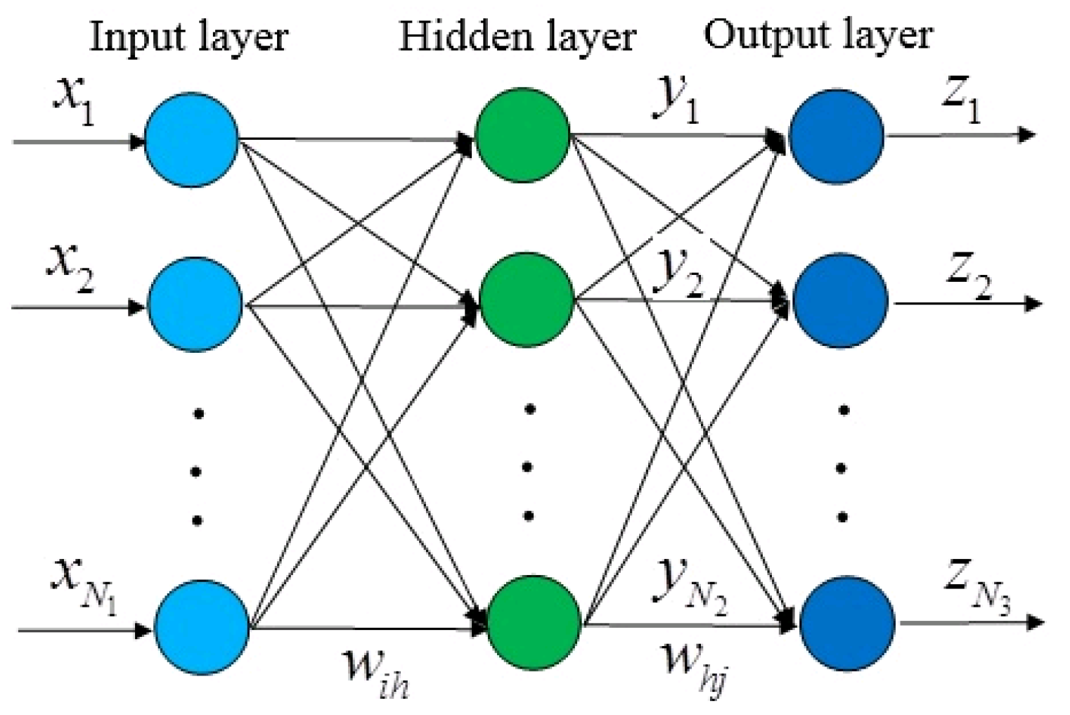
Artificial neural network (ANN) is a classical fundamental technique in machine learning. Compared with general multi-factor prediction methods, its prediction method has the advantages of high fault tolerance, high reliability, and fast prediction speed. In addition, ANN is a powerful interpolation tool [64,65,66]. Artificial neural networks generally have more than three layers of multilayer neural networks, which generally include three-layer structures of input, hidden, and output layers, as shown in Figure 4.
The relationship between the input and output of neurons is , where is the net activation, is the input vector, is the weight vector, and is the activation function, which represents the function of mapping the net activation and output. Some commonly used activation functions include , , , etc.
A neural network can be divided into two states: learning state and working state. The learning state is used to adjust the weight of the neural network to make the output close to the actual value, while the working state uses the established network for classification and prediction without changing the weight of the neural network. The learning mode of the neural network is tutorial learning. The weight of the network is adjusted by the difference between the actual output and expected output of the network to make the model adapt as accurately as possible.
In this study, the MLP neural network was used to estimate the missing values from the water quality data of the Jinjiang River. The activation function of the output layer is constant. The single-layer perceptron is the simplest neural network, which is composed of input and output layers, and the input and output layers are directly connected. The MLP neural network contains an input layer, output layer, and several hidden layers, which is a kind of multi-layer feed-forward neural network based on BP algorithm training. The input signal is passed forward through the input layer to the hidden layer, and subsequently the neurons in the hidden layer are computationally processed and then passed forward to the output layer, which is a forward transmission process in which the output of the MLP neural network depends only on the current input and not on past or future inputs; thus, the MLP neural network is also known as a multi-layer feed-forward neural network. Among many neural network architectures, MLP neural networks are simple in structure, easy to implement, and have good fault tolerance, robustness, and excellent nonlinear mapping capability (Figure 5).
2.5. Basic Principle of Wavelet Transform
In the process of time-series data acquisition, there will be some noise in the time series data due to observation error, systematic error, or other reasons, and the noise will seriously affect the data processing results. Therefore, in the data preprocessing stage, different methods should be selected to denoise the data according to the type of noise. Common denoising methods include the Fourier transform [67], the wavelet transform [68], etc.
The Fourier transform is a widely used analysis method in the field of signal processing. It converts a time domain signal into a frequency domain signal. Its basic idea is to decompose the signal into the superposition of a series of continuous sine waves with different frequencies. However, Fourier transform also has many disadvantages. The traditional Fourier transform can only realize the overall transformation between the signal time domain and the frequency domain and cannot distinguish time-domain information. However, Fourier transform is only suitable for stable signals; most signals have variability, which significantly limits the application of Fourier transform.
The basic idea of wavelet transform is to adaptively adjust the time-frequency window according to the signal, decomposing the original signal into a series of sub-band signals with different spatial resolutions, frequency characteristics, and directional characteristics after stretching and translating. These sub-bands have good local characteristics in both the time and frequency domains and can therefore be used to represent the local characteristics of the original signal, thus enabling the localization of the signal in time and frequency. This method can overcome the limitations of Fourier analysis in dealing with non-smooth signals and complex images.
The mathematical definition of wavelet is as follows: let , which is almost always 0 on R and satisfies , then is the wavelet, where is the Fourier transform of . Wavelet transform is one order of magnitude faster than fast Fourier transform. When the signal length is M, the computational complexity of Fourier transform is Of = Mlog2M and that of wavelet transform is OM = M.
Wavelet transform can be divided into continuous wavelet transform (CWT) and discrete wavelet transform (DWT).
The formula of continuous wavelet transform is:
where Wf(a,b) is the continuous wavelet coefficient, a is the scaling factor, b is the translation factor, is the conjugate function of , and represents the original data. The scale of wavelet transform is controlled by adjusting the values of a and b to realize the adaptive time-frequency signal analysis.
The discrete wavelet transform formula is:
where Wf(j,k) is the discrete wavelet coefficient and f(t) is the original data.
The dbn wavelet is the most common wavelet transform and is mainly used in discrete wavelet transform. For wavelets of a finite length, when applied to fast wavelet transform, there will be a sequence composed of two real numbers. One is the coefficient of the high-pass filter, which is called the wavelet filter, and the other is the coefficient of the low-pass filter, which is called the adjustment filter. Firstly, the wavelet transform decomposes the original data into the low-frequency wavelet coefficient cAn and high-frequency wavelet coefficient cD1, cD2, …, cDn by using the low-pass filter and high-pass filter, respectively. Among them, the low-frequency wavelet coefficient can be further decomposed and iterated several times until the maximum decomposition time is reached. Finally, the decomposed wavelet low-frequency signal and high-frequency signal are added to realize wavelet reconstruction. The formula is:
where f(t) is the restored signal; and are the low-pass filter and high pass filter, respectively; cAn is low-frequency wavelet coefficient; and cDn is high-frequency wavelet coefficient.
The calculation steps of wavelet transform are as follows:
Step 1. Elect the wavelet function and align it with the starting point of the analysis signal.
Step 2. Calculate the approximation degree between the signal to be analyzed and the wavelet function at this time; that is, the wavelet transform’s coefficient C. The larger the coefficient C, If the coefficient C is larger, the more similar the current signal is to the waveform of the selected wavelet function.
Step 3. Move the wavelet function to the right one-unit time along the time axis, and then repeat Steps 1 and 2 to calculate the transformation coefficient C until it covers the whole signal length.
Step 4. Scale the selected wavelet function by one unit, and then repeat Steps 1–4.
Step 5. Repeat Steps 1–4 for all expansion scales.
The selection of the mother wavelet type and decomposition level are the two most important problems in wavelet analysis. In this study, the db5 wavelet was used to decompose the experimental sequence for the following two reasons:
- (1)
- The db wavelets are more suitable for relatively stable sequences;
- (2)
- db5 is also one of the most commonly used wavelets in the db wavelet family, which is suitable for smoother datasets.
Because Jinjiang water quality data has obvious smoothing characteristics, the db5 wavelet analysis was the most suitable method for this study.
The maximum decomposition levels of wavelet can be calculated by the following Equation (5):
where lw is the length of the wavelet decomposition low-pass filter and nd is the data length.
L = ln(nd/(lw − 1))
In this study, lw = 23 and nd = 443 were selected, and L was calculated such that the number of wavelet decomposition layers was 3.
2.6. Basic Principle of LSTM
RNN was first proposed in the 1980s. As a popular algorithm in deep learning, compared with deep learning network (DNN), its circular network structure allows it to take full advantage of the sequence information in the sequence data itself. Therefore, it has many advantages in dealing with time series. Moreover, the ability to correct errors is achieved through back-propagation and a gradient descent algorithm. However, there are also many problems: as the time series grows, researchers have found that RNNs are weak for long time series, which means that the long-term memory of RNNs is poor. At the same time, as the length of the sequence increases, the depth of the model increases, and the problem of gradient disappearance and gradient explosion cannot be avoided when calculating the gradient. Therefore, Hochreiter et al. [69] proposed LSTM. The structure of LSTM is shown in Figure 6 [70].
The long-short term memory network is different from the traditional recurrent neural network in rewriting memory at each time step. LSTM will save the important features it has learned as long-term memory, and selectively retain, update, or forget the saved long-term memory according to the learning. However, the features with small weight in multiple iterations will be regarded as short-term memory and eventually forgotten by the network. This mechanism allows the important feature information to be transmitted all the time with the iteration so that the network has better performance in the classification task with a long-time dependence of samples. LSTM has been widely applied in flood sensitivity prediction [71], the prediction of key parameters of nuclear power plants [72], wind speed prediction [73,74], financial price trends [75], language processing [76], etc. In recent years, the LSTM model has made a series of improvements on the basis of RNN neurons. These include the addition of a transmission unit state in the RNN hidden layer controlled by three gating units: the forgetting gate, input gate, and output gate. Forgetting gates are used to control the forgetting of information and the extent to which it is retained. The calculation formula is:
where Xt is the current input information, ht−1 is the data information in the previous hidden state, and the range of Ft is 0 to 1. When Ft = 1, it means that the information is completely retained, and when Ft = 0, it means that the information is completely abandoned.
The input gate is used to control how much input information at the current time is saved to the unit state. The expression is written as:
where Wi is the weight matrix, bi is the offset term, and It is the input layer vector value.
The input unit status Ct is represented as:
where Wc is the weight matrix and bc is the offset term.
The output calculation formula of the output gate Ot is shown as:
where bo is the offset value, Wo is the judgment matrix, and ht−1 is the hidden layer state at time (t−1).
In Equation (11), is the Hadamard product and ht is the hidden layer state at time t.
2.7. Evaluation Index
In this study, mean square error (MSE), root mean square error (RMSE), mean absolute error (MAE), and mean percentage error (MAPE) were selected as the basis for judging the prediction effect of the model. The calculation formulae are as follows:
where N represents the total data volume, represents the real value, and represents the predicted value.
MAE is used to measure the mean absolute error between the predicted and actual values, RMSE is used to measure the deviation between the predicted and actual values (which is sensitive to outliers), and MAPE is used to measure the average relative error between the predicted and actual values.
3. Results
3.1. Artificial Neural Network Interpolation
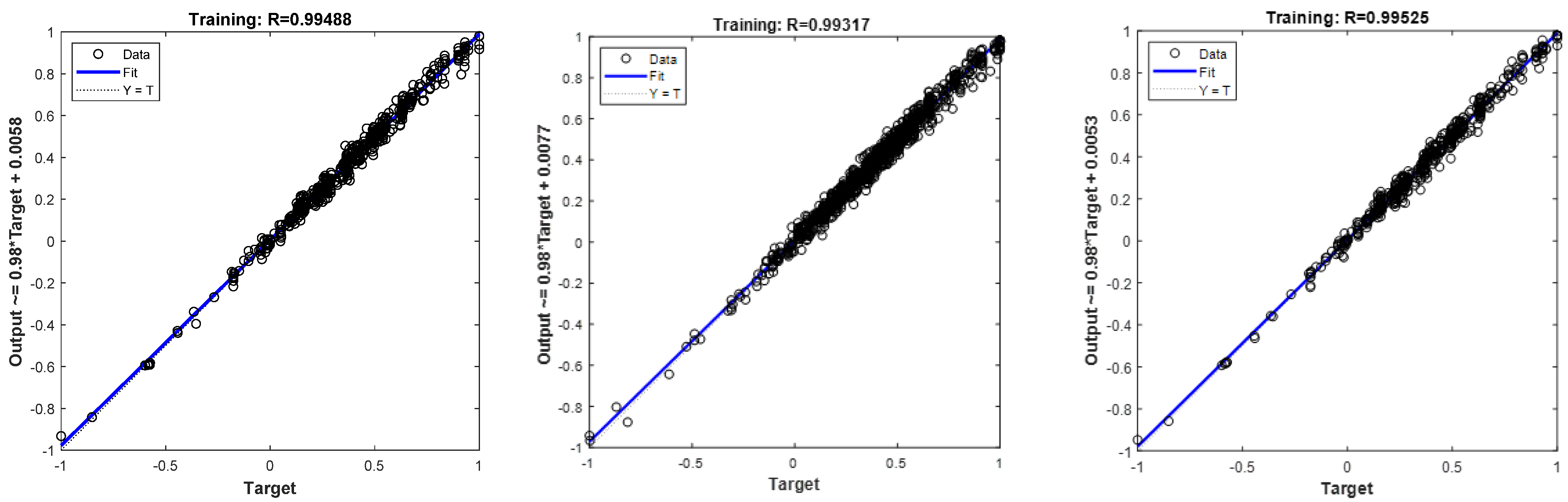
In this study, we used MATLAB to construct a multilayer perceptron neural network to fill in the missing data in each dataset. The parameters of MLP were set as follows: the number of implied layers was two, the optimization algorithm was the conjugate scalar gradient algorithm, and the minimum relative change in the training error rate was 0.001. The artificial neural network training images for the DO, CODMn, and NH3-N datasets are shown in the Figure 7.
As shown in Figure 7, the coefficient of determination was 0.99488 for the DO dataset, 0.99317 for the CODMn dataset, and 0.99525 for the NH3-N dataset. It is clear that the fit of each dataset was good. Therefore, the model could be used to estimate the missing values in the DO, CODMn, and NH3-N datasets.
3.2. Results of Wavelet Transform Model
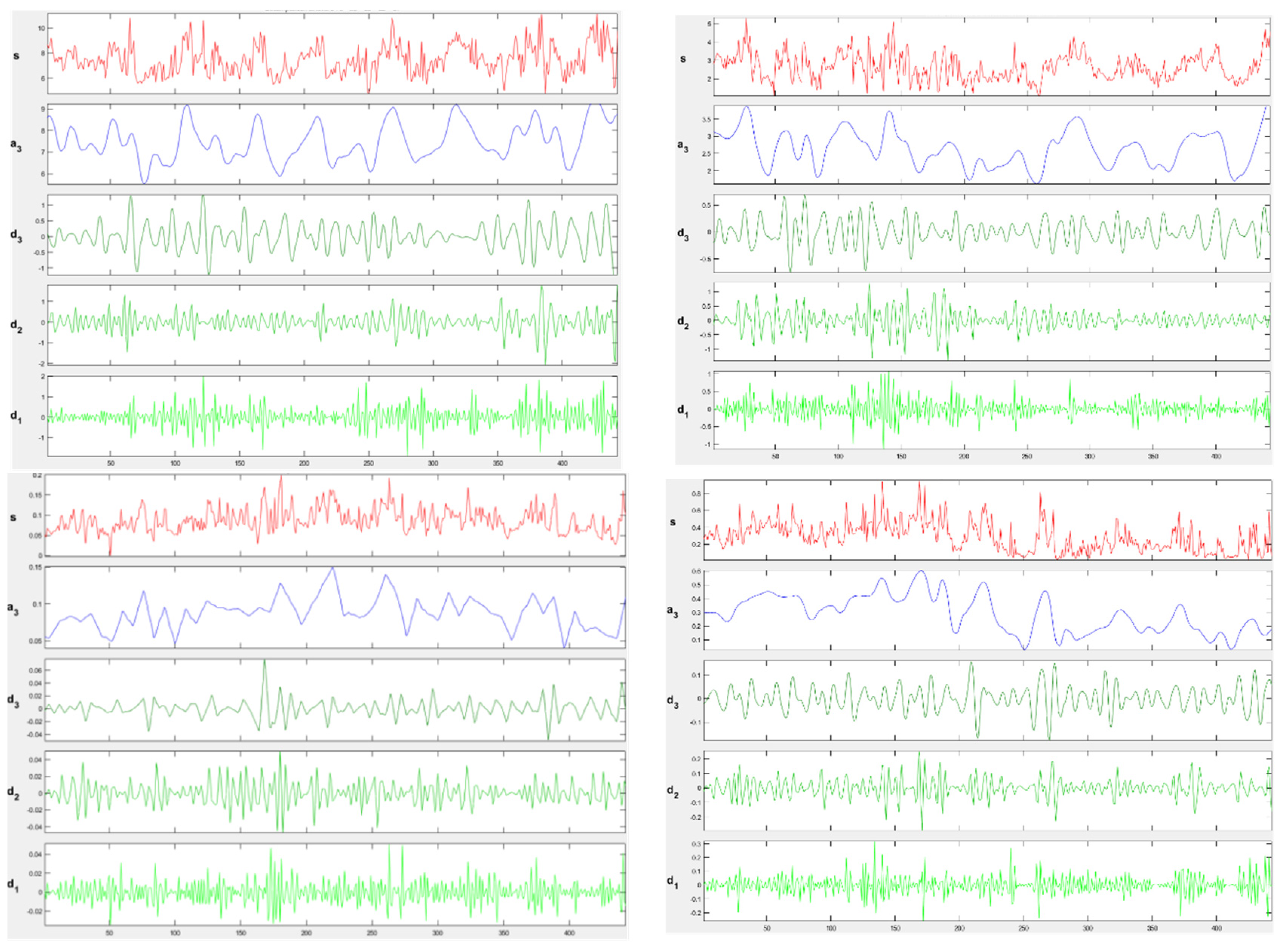
Figure 8 shows the original images of DO, CODMn, TP and NH3-N and the images after db5 wavelet decomposition.
However, after summing the data signals of each frequency band after wavelet reconstruction into the original signal, there is a certain error between this reduced data and the original data that is determined by the characteristics of the computer and is an error that cannot be eliminated. If this error value is too large, the experimental results will not be credible. Therefore, in this research, in order to verify the experimental accuracy of the model, the difference between the reduced data and the original data after wavelet reconstruction of the four indicators in the experiment was calculated. The errors are shown in Table 4.
From Table 4, it can be found that the error of CODMn was the largest (6.75 × ) and the error of DO was the smallest (9.1 × ). An error value in this range interval has a negligible effect on the experimental results, which proves the validity of the experiment.
3.3. Model Result Output
After wavelet transform of DO, CODMn, TP, and NH3-N data, the decomposed low-frequency wavelet coefficient cA and high-frequency wavelet coefficient cD were used as the input of LSTM. Meanwhile, in order to verify that the ANN-WT-LSTM model had a higher prediction accuracy than other models, we selected ANN-LSTM, ARIMA, and NAR neural network models for comparison. The parameter settings of the other models are shown in Table 5.
3.4. Comparison with Other Models
We aimed to compare the prediction results of the ANN-WT-LSTM model with other existing models, compare the prediction accuracy of the different models, and analyze the prediction efficiency of the models. The comparison results of the model predictions are shown in Table 6.
4. Discussion
Water pollution is one of the biggest important environmental problems facing mankind, and the harm caused by it is largely due to the lack of prediction and early warning and emergency disposal capabilities. Therefore, the construction of an effective monitoring and early warning system to achieve intelligent decision making and the management of water quality is a key scientific and technological issue that needs to be addressed urgently. However, because water quality indicators usually have the characteristics of nonlinearity and non-smoothness, conventional statistical models often have difficulties making accurate predictions [77]. In recent years, there has been a rapid development of deep learning technology and wireless sensing technology. The model proposed in this study can be applied in the following aspects:
- (1)
- Existing monitoring systems cannot achieve online high-frequency monitoring of all important pollutants, so the model proposed in this study can be used for soft computing to improve the timeliness, coverage and frequency of online monitoring and to form an effective early warning system for water quality management.
- (2)
- According to real-time monitoring data for water quality change trend prediction and water quality risk judgment. When the prediction results show that the water quality situation has a deteriorating trend, the relevant management departments can make the corresponding measures of pollution prevention and control at the first time, so as to minimize the water quality losses caused by pollution incidents.
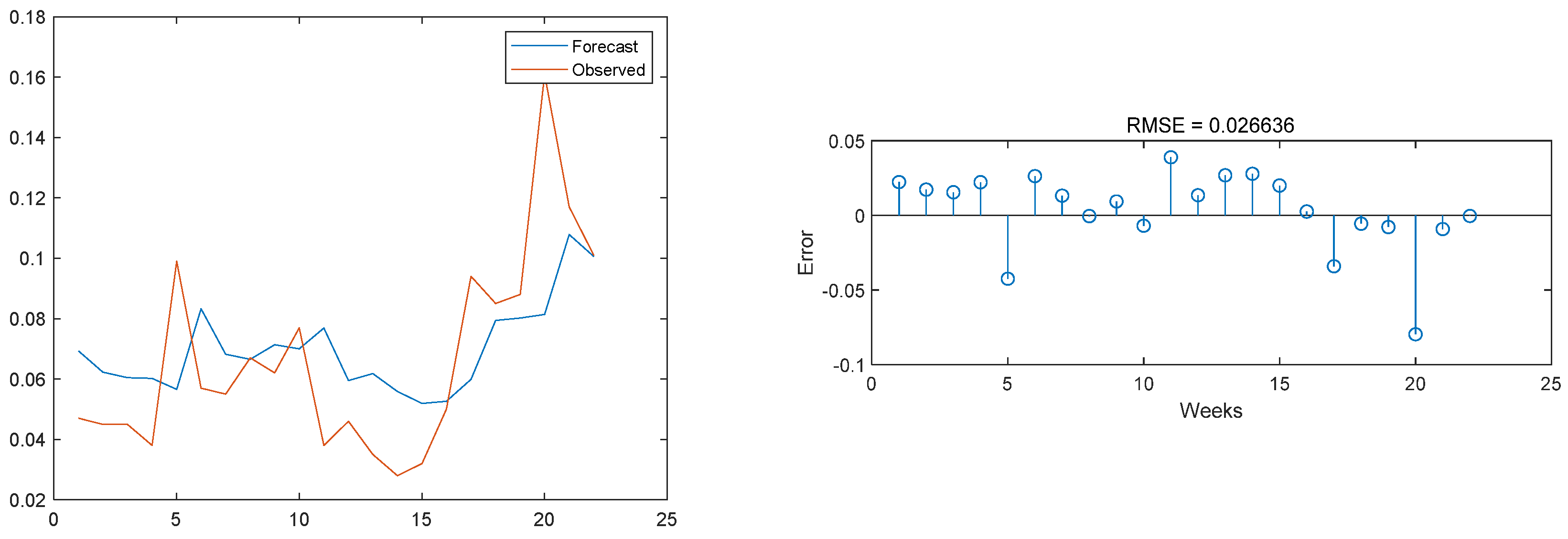
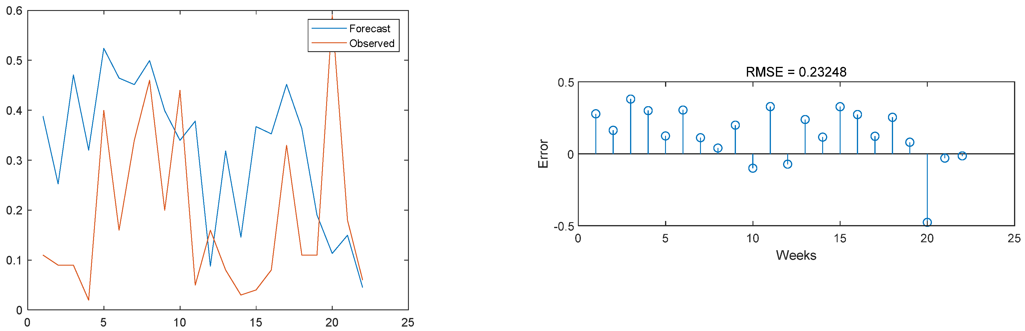
From the above results and error images, it can be seen that the accuracy of the ANN-WT-LSTM model prediction on the DO dataset was substantially improved compared with the MLPNN model, ANN-LSTM model, NAR neural network model, CNN-LSTM model, SSA-LSTM, SSA-BPNN model, and ISSA-BPNN model. For the CODMn dataset, the MAPE of the ANN-WT-LSTM model was 0.021, which was 0.157, 0.2383, 0.1749, 0.677, 0.129, 1.569, 0.139, 1.279, 0.749, 0.029, and 0.039 lower compared to the ANN-LSTM model, NAR neural network model, ARIMA model, MLPNN model, CNN-LSTM model, BPNN model, SSA-LSTM model, ISSA-BPNN model, SSA-BPNN model, DWT-CNN-LSTM model, and EMD-LSTM model, respectively. For the TP dataset, the RMSE of the ANN-WT-LSTM model was 0.026, which decreased by 0.004, 0.0085, 0.0099, 0.007, 0.108, 0.424, 0.114, 0.324, 0.334, 0.019, and 0.164, respectively, compared to the other models. For the NH3-N dataset, the MSE of the ANN-WT-LSTM model was 0.006, which decreased by 0.024, 1.939, 0.0237, 0.009, 0.002, 0.064, 0.003, 0.044, 0.094, 0.024, and 0.016, respectively, when compared with the other models.
It is known that water quality prediction methods are divided into two main categories: mechanistic and non-mechanistic predictions. Mechanistic water quality models are derived using system structure data based on constraints in the underlying physical, biological, and chemical processes of the water environment system. A variety of water quality models have been developed, such as QUAL, WASP, MIKE, EFDC, SWAT, SMS, BASINS, etc., and have been widely used. However, these mechanistic water quality models are very complex and require a large amount of basic data information (such as simulation parameters, source and sink terms, etc.) to establish and solve the water quality control equations. This makes the complexity of building water quality models high and the parameters more difficult to determine, leading to limitations in the application of the models in many water bodies [78,79]. Moreover, for many aquatic environmental systems, the detailed mechanisms are not fully explained, and the evolutionary development of water quality is influenced and disturbed by many variables, such as physics, chemistry, biology, meteorology, and hydraulics, with strong non-linear characteristics. The existing water quality prediction models based on mathematical expressions are unable to take the influence of these factors into account, and it is difficult to accurately describe the migration and dispersion of the water environment using mechanistic modelling; hence, the predictions made on this basis have a “natural” bias. Furthermore, typical basin hydrological models, such as SWAT, HSPF and MIKE, have different scenarios that are able to simulate the hydrological processes and the evolution of point and non-point sources of pollution in large scale basins over long periods of time; however, they are not suitable for predicting water quality in larger water bodies, such as lakes and reservoirs. Water quality models such as CE-QUAL-W2, WASP, and EPD-RIV1 address the hydrodynamics and water quality of larger water bodies, but not the hydrological problems that occur in the basin.
In contrast, the ANN-WT-LSTM model proposed in this paper is based on the idea of neural networks to analyze historical water quality data to predict future water quality changes, and is one of the non-mechanical water quality prediction methods. Non-mechanical forecasting methods use the idea of statistics, through the water quality related to the historical time series data mining analysis, to find its data behind the law of change, and then deduce the trend of water quality changes. Compared with the mechanistic water quality prediction methods, the advantages are obvious. First of all, the modelling cost is lower as the modelling data requirements are not high. Therefore, the method can be applied to water quality prediction in areas where a large amount of hydrological data is missing. Secondly, the model prediction reliability is good, because the ANN-WT-LSTM model has good applicability to the analysis and prediction of non-linear problems in uncertain environment; thus, the water quality prediction accuracy has been improved a great deal compared with previous models (Table 6). In addition, the ANN-WT-LSTM model has good applicability. The model itself is a “black box” model analysis, which does not need the hydrological data of pollution sources for analysis. Whether the study area is the river basin environment or lakes, reservoirs or other large water bodies, it has wide applicability and universality. In summary, our view is that the ANN-WT-LSTM model proposed in this paper is not the only choice in water quality prediction models, but it still has great potential for application compared to other competing methods (including 1D, 2D, and 3D numerical models) due to its reliability, efficiency, and accuracy.
The ANN-DWT-LSTM model proposed in this study still has several aspects that can be improved.
- (1)
- The model proposed in this paper only considers the historical data of water quality indicators in the Jinjiang River basin, while changes in the external environment have a greater impact on river water quality, which can interfere with the neural network training process, thus affecting the accuracy of the model. There is still room for further research into how to reduce the interference of external factors or consider the influence of water quality factors in the model.
- (2)
- In this study, LSTM was used to predict water quality; however, there are numerous improved versions of the LSTM model, including the Bi-LSTM (bi-directional long short-term memory network) and the adaptive neuro-fuzzy inference system (ANFIS). These methods can be used to compare with the model proposed in this study.
Based on the powerful parallel data processing capability and non-linear processing ability of neural networks, we believe that the model proposed in this study can be combined with big data technologies, such as IoT, which can process large-scale data quickly and accurately and can meet the requirements of multi-sensor data fusion well.
5. Conclusions
To improve the accuracy of water quality prediction data, this study proposed the ANN-WT-LSTM model based on an artificial neural network, wavelet transform, and long short-term memory network, using the water quality data of the Jinjiang River basin in China as the research object for prediction analysis. For missing water quality data caused by instrument failure, this study used an artificial neural network to fill in the missing values based on the time-series information of water quality data. Then, we used wavelet transform to decompose and reconstruct the water quality time series, in order to remove the impact of short-term random disturbance noise, improve the prediction accuracy of the model on out-of-sample data, and the ability to predict future dynamic trends, so that it can more effectively predict the short-term as well as long-term dynamic trends in water quality time-series data. Subsequently, compared with the ANN-LSTM model and the NAR neural network model, the results show that the ANN-WT-LSTM proposed in this study is better than other models in all evaluation indexes, and the model effectively improves the accuracy of water quality prediction, which is significant for water environment protection. The study not only provides vital data support for water quality safety management decisions, but also has important theoretical and practical significance for safeguarding the sustainable development of the riverine areas and water environmental protection in the reservoir area.
This study predicts the possible future situation of reservoir water quality through the study of time series. However, due to the limitation of monitoring conditions, it can only predict the water quality at one point of the reservoir, which cannot reflect the overall spatial change of water quality. Therefore, in order to establish a more perfect reservoir early warning system, we suggest that water quality monitoring points be set up in many places to monitor the water quality in different directions of the reservoir to combine water quality prediction with GIS technology. In this way, we not only study the development trend of water quality in time, but also study the change of water quality in space, so as to combine time and space prediction and lay a good foundation for establishing a perfect water quality early warning system.
Author Contributions
Conceptualization, J.W.; methodology, J.W. and Z.W.; supervision, J.W.; investigation, J.W.; visualization, J.W.; writing—original draft, J.W. and Z.W.; writing—review and editing, J.W. and Z.W.; validation, J.W. and Z.W.; diagram and flowchart preparation, Z.W. All authors have read and agreed to the published version of the manuscript.
Funding
This research was supported by the Open Research Fund of the State Key Laboratory of Simulation and Regulation of Water Cycle in River Basin, China Institute of Water Resources and Hydropower Research (grant No. IWHR-SKL-201905).
Institutional Review Board Statement
Not applicable.
Informed Consent Statement
Not applicable.
Data Availability Statement
The data presented in this study are available on request from the corresponding authors. The data are not publicly available due to the continuation of a follow-up study by the authors.
Acknowledgments
We would like to thank the computing science center of Shanghai Ocean University for its support in the scientific research.
Conflicts of Interest
The authors declare no conflict of interest.
References
- Wang, Q.; Hao, D.; Li, F.; Guan, X.; Chen, P. Development of a new framework to identify pathways from socioeconomic development to environmental pollution. J. Clean Prod. 2020, 253, 119962. [Google Scholar] [CrossRef]
- Ministry of Water Resources. Water Resources Assessment in China; Water and Hydropower Publishing: Beijing, China, 2018; pp. 154–196.
- Shi, X. The Safety of Drinking Water in China: Current Status and Future Prospects. China CDC Wkly. 2020, 2, 210–215. [Google Scholar] [CrossRef] [PubMed]
- Hara, J.; Mamun, M.; An, K. Ecological river health assessments using chemical parameter model and the index of biological integrity model. Water 2019, 11, 1729. [Google Scholar] [CrossRef] [Green Version]
- Chen, X.; Strokal, M.; Van, V.; Michelle, T.; Stuiver, J.; Wang, M.; Bai, Z.; Kroeze, C.; Ma, L. Multi-scale Modeling of Nutrient Pollution in the Rivers of China. Environ. Sci. Technol. 2019, 53, 9614–9625. [Google Scholar] [CrossRef] [PubMed] [Green Version]
- Huang, J.; Zhang, Y.; Bing, H.; Peng, J.; Arhonditsis, G. Characterizing the river water quality in china: Recent progress and on-going challenges. Water Res. 2021, 201, 117309. [Google Scholar] [CrossRef] [PubMed]
- Sarpong, K.; Xu, W.; Mensah-Akoto, J.; Neequaye, J.; Dadzie, A.; Frimpong, O. Waterscape, State and Situation of China’s Water Resources. J. Geosci. Environ. Prot. 2020, 8, 26–51. [Google Scholar] [CrossRef]
- O’Connor, D. Oxygen Balance of an Estuary. Tran. Am. Soc. Civ. Eng. 1961, 126, 556–575. [Google Scholar] [CrossRef]
- Thomann, R. Mathematical Model for Dissolved Oxygen. J. Sanit. Eng. Div. 1963, 89, 1–32. [Google Scholar] [CrossRef]
- Dobbins, W. BOD and Oxygen Relationship in Streams. J. Sani. Eng. Div. 1964, 90, 53–78. [Google Scholar] [CrossRef]
- Ma, W.; Chao, Z. The numerical simulation of water quality of Suzhou Creek based on GIS. Acta Geogr. Sin. 1998, 53, 66–75. [Google Scholar]
- Zhang, Y.; Xia, J.; Shao, Q.; Zhai, X. Water quantity and quality simulation by improved SWAT in highly regulated Huai River Basin of China. Stoch. Env. Res. Risk Assess. 2013, 27, 11–27. [Google Scholar] [CrossRef]
- Peng, S.; Fu, G.; Zhao, X.; Moore, B. Integration of Environmental Fluid Dynamics Code (EFDC) Model with Geographical Information System (GIS) Platform and Its Applications. J. Environ. Inform. 2011, 17, 75–82. [Google Scholar] [CrossRef]
- Huang, M.; Tian, Y. An Integrated Graphic Modeling System for Three-Dimensional Hydrodynamic and Water Quality Simulation in Lakes. ISPRS Int. J. Geo-Inf. 2019, 8, 18. [Google Scholar] [CrossRef] [Green Version]
- Lee, I.; Hwang, H.; Lee, J.; Yu, N.; Yun, J.; Kim, H. Modeling approach to evaluation of environmental impacts on river water quality: A case study with Galing River, Kuantan, Pahang, Malaysia. Ecol. Model. 2017, 353, 167–173. [Google Scholar] [CrossRef]
- Deus, R.; Brito, D.; Mateus, M.; Kenov, I.; Fornaro, A.; Neves, R.; Alves, C. Impact evaluation of a pisciculture in the Tucuruí reservoir (Pará, Brazil) using a two-dimensional water quality model. J. Hydrol. 2013, 487, 1–12. [Google Scholar] [CrossRef]
- Al-Zubaidi, H.A.M.; Wells, S.A. Analytical and field verification of a 3D hydrodynamic and water quality numerical scheme based on the 2D formulation in CE-QUAL-W2. J. Hydraul. Res. 2018, 58, 152–171. [Google Scholar] [CrossRef] [Green Version]
- Yang, L.K.; Peng, S.; Zhao, X.H.; Li, X. Development of a two-dimensional eutrophication model in an urban lake (China) and the application of uncertainty analysis. Ecol. Model. 2017, 345, 63–74. [Google Scholar]
- Colton, B.; Tassiane, J.; Alice, D.; Bas, V. Mass-Balance Modeling of Metal Loading Rates in the Great Lakes. Environ. Res. 2022, 205, 112557. [Google Scholar]
- Wang, X.; Jia, J.; Su, T.; Zhao, Z.; Xu, J.; Li, W. A fusion water quality soft-sensing method based on wasp model and its application in water eutrophication evaluation. J. Chem. 2018, 2018, 9616841. [Google Scholar] [CrossRef] [Green Version]
- Yang, H.; Wang, J.; Li, J.; Zhou, H.; Liu, Z. Modelling impacts of water diversion on water quality in an urban artificial lake. Environ. Pollut. 2021, 276, 116694. [Google Scholar] [CrossRef]
- Najafzadeh, M.; Noori, R.; Afroozi, D.; Ghiasi, B.; Hosseini-Moghari, S.M.; Mirchi, A.; Haghighi, A.T.; Kløve, B. A comprehensive uncertainty analysis of model-estimated longitudinal and lateral dispersion coefficients in open channels. J. Hydrol. 2021, 603, 126850. [Google Scholar] [CrossRef]
- Song, C.; Yao, L.; Hua, C.; Ni, Q. A novel hybrid model for water quality prediction based on synchrosqueezed wavelet transform technique and improved long short-term memory. J. Hydrol. 2021, 603, 126879. [Google Scholar] [CrossRef]
- Noori, R.; Safavi, S.; Shahrokni, S.A.N. A reduced-order adaptive neuro-fuzzy inference system model as a software sensor for rapid estimation of five-day biochemical oxygen demand. J. Hydrol. 2013, 495, 175–185. [Google Scholar] [CrossRef]
- Noori, R.; Karbassi, A.R.; Ashrafi, K.; Ardestani, M.; Mehrdadi, N. Development and application of reduced-order neural network model based on proper orthogonal decomposition for BOD5 monitoring: Active and online prediction. Environ. Prog. Sustain. Energy 2013, 32, 120–127. [Google Scholar] [CrossRef]
- Noori, R.; Yeh, H.D.; Abbasi, M.; Kachoosangi, F.T.; Moazami, S. Uncertainty analysis of support vector machine for online prediction of five-day biochemical oxygen demand. J. Hydrol. 2015, 527, 833–843. [Google Scholar] [CrossRef]
- Ahmed, U.; Mumtaz, R.; Anwar, H.; Shah, A.; García-Nieto, J. Efficient Water Quality Prediction Using Supervised Machine Learning. Water 2019, 11, 2210. [Google Scholar] [CrossRef] [Green Version]
- Liu, P.; Wang, J.; Sangaiah, A.; Xie, Y.; Yin, X. Analysis and Prediction of Water Quality Using LSTM Deep Neural Networks in IoT Environment. Sustainability 2019, 11, 2058. [Google Scholar] [CrossRef] [Green Version]
- Hu, Z.; Zhang, Y.; Zhao, Y.; Xie, M.; Zhong, J.; Tu, Z.; Liu, J. A water quality prediction method based on the deep LSTM network considering correlation in smart mariculture. Sensors 2019, 19, 1420. [Google Scholar] [CrossRef] [Green Version]
- Eze, E.; Halse, S.; Ajmal, T. Developing a Novel Water Quality Prediction Model for a South African Aquaculture Farm. Water 2021, 13, 1782. [Google Scholar] [CrossRef]
- Solanki, A.; Agrawal, H.; Khare, K. Predictive Analysis of Water Quality Parameters using Deep Learning. Int. J. Comput. Appl. 2015, 125, 29–34. [Google Scholar] [CrossRef] [Green Version]
- Wang, J.; Zhang, L.; Zhang, W.; Wang, X. Reliable Model of Reservoir Water Quality Prediction Based on Improved ARIMA Method. Environ. Eng. Sci. 2019, 36, 1041–1048. [Google Scholar] [CrossRef]
- Abdel-Fattah, M.; Mokhtar, A.; Abdo, A. Application of neural network and time series modeling to study the suitability of drain water quality for irrigation: A case study from Egypt. Environ. Sci. Pollut. R. 2021, 28, 898–914. [Google Scholar] [CrossRef] [PubMed]
- Shi, B.; Peng, W.; Jiang, J.; Liu, R. Applying high-frequency surrogate measurements and a wavelet-ANN model to provide early warnings of rapid surface water quality anomalies. Sci. Total Environ. 2018, 1390, 610–611. [Google Scholar] [CrossRef] [PubMed]
- Li, X.; Cheng, Z.; Yu, Q.; Bai, Y.; Li, C. Water-Quality Prediction Using Multimodal Support Vector Regression: Case Study of Jialing River, China. J. Environ. Eng. 2017, 143, 4017070. [Google Scholar] [CrossRef]
- Ewaid, S.; Abed, S.; Kadhum, S. Prediction the Tigris river water quality within Baghdad, Iraq by using water quality index and regression analysis. Environ. Technol. Innov. 2018, 11, 390–398. [Google Scholar] [CrossRef]
- Xu, L.; Liu, S. Study of short-term water quality prediction model based on wavelet neural network. Mat. Comput. Model. 2013, 58, 801–807. [Google Scholar] [CrossRef]
- Long, S. Study of Short-term Water Quality Prediction Model Based on PSO-WSVR. J. Zhengzhou Univ. 2013, 58, 807–813. [Google Scholar]
- Tizro, A.; Ghashghaie, M.; Georgiou, P.; Voudouris, K. Time series analysis of water quality parameters. J. Appl. Res. Water Wastewater 2014, 1, 43–52. [Google Scholar]
- Faruk, D. A hybrid neural network and ARIMA model for water quality time series prediction. Eng. Appl. Artif. Intel. 2010, 23, 586–594. [Google Scholar] [CrossRef]
- Zhang, L.; Zhang, G.; Li, R. Water Quality Analysis and Prediction Using Hybrid Time Series and Neural Network Models. J. Agric. Sci. Tech. IRAN 2016, 18, 975–983. [Google Scholar]
- Than, N.; Ly, C.; Tat, P. The performance of classification and forecasting Dong Nai River water quality for sustainable water resources management using neural network techniques. J. Hydrol. 2021, 596, 126099. [Google Scholar] [CrossRef]
- Zhou, J.; Wang, Y.; Xiao, F.; Wang, Y.; Sun, L. Water Quality Prediction Method Based on IGRA and LSTM. Water 2018, 10, 1148. [Google Scholar] [CrossRef] [Green Version]
- Hameed, M.; Sharqi, S.; Yaseen, Z.; Afan, H.; Hussain, A.; Elshafie, A. Application of artificial intelligence (AI) techniques in water quality index prediction: A case study in tropical region, Malaysia. Neural Comput. Appl. 2017, 28, 893–905. [Google Scholar] [CrossRef]
- Deng, J.; Guo, P.; Zhang, X.; Shen, X.; Su, H.; Zhang, Y.; Wu, Y.; Xu, C. An evaluation on the bioavailability of heavy metals in the sediments from a restored mangrove forest in the Jinjiang Estuary, Fujian, China. Ecotox. Environ. Safe. 2019, 180, 501–508. [Google Scholar] [CrossRef] [PubMed]
- Liu, X.; Jiang, J.; Yan, Y.; Dai, Y.; Deng, B.; Ding, S.; Su, S.; Sun, W.; Li, Z.; Gan, Z. Distribution and risk assessment of metals in water, sediments, and wild fish from Jinjiang River in Chengdu, China. Chemosphere 2018, 196, 45–52. [Google Scholar] [CrossRef]
- Chen, P. Effects of normalization on the entropy-based TOPSIS method. Expert Syst. Appl. 2019, 136, 33–41. [Google Scholar] [CrossRef]
- Alkhodari, M.; Fraiwan, L. Convolutional and recurrent neural networks for the detection of valvular heart diseases in phonocardiogram recordings. Comput. Methods Prog. Bio. 2021, 200, 105940. [Google Scholar] [CrossRef]
- Newman, D. Missing data: Five practical guidelines. Organ. Res. Methods 2014, 17, 372–411. [Google Scholar] [CrossRef]
- Little, R.; Rubin, D. Statistical Analysis with Missing Data, 2nd ed.; John Wiley & Sons: Hoboken, NJ, USA, 2014. [Google Scholar]
- Little, R.; Rubin, D. The analysis of social science data with missing values. Sociol. Method Res. 1989, 18, 292–326. [Google Scholar] [CrossRef]
- Shan, Y.; Deng, G. Kernel PCA regression for missing data estimation in DNA microarray analysis. In Proceedings of the 2009 IEEE International Symposium on Circuits and Systems, Taipei, Taiwan, 24–27 May 2009; pp. 1477–1480. [Google Scholar]
- Wang, Z.; Wu, X.; Wang, H.; Wu, T. Prediction and analysis of domestic water consumption based on optimized grey and Markov model. Water Supply 2021, 21, 3887–3899. [Google Scholar] [CrossRef]
- Wu, J.; Wang, Z.; Dong, L. Prediction and analysis of water resources demand in Taiyuan City based on principal component analysis and BP neural network. J. Water Supply Res. Tech. 2021, 70, 1272–1286. [Google Scholar] [CrossRef]
- Wu, X.; Wang, Z.; Wu, T.; Bao, X. Solving the Family Traveling Salesperson Problem in the Adleman-Lipton model based on DNA computing. IEEE Trans. Nanobiosci. 2022, 21, 75–85. [Google Scholar] [CrossRef] [PubMed]
- Noori, R.; Karbassi, A.R.; Mehdizadeh, H.; Vesali-Naseh, M.; Sabahi, M.S. A framework development for predicting the longitudinal dispersion coefficient in natural streams using an artificial neural network. Environ. Prog. Sustain. 2011, 30, 439–449. [Google Scholar] [CrossRef]
- Wang, Z.; Bao, X.; Wu, T. A Parallel Bioinspired Algorithm for Chinese Postman Problem Based on Molecular Computing. Comput. Intel. Neurosc. 2021, 2021, 8814947. [Google Scholar] [CrossRef]
- Austin, C.; White, R.; Buuren, V. Missing Data in Clinical Research: A Tutorial on Multiple Imputation. Can. J. Cardiol. 2020, 37, 1322–1331. [Google Scholar] [CrossRef] [PubMed]
- Chang, C.; Deng, Y.; Jiang, X.; Long, Q. Multiple imputation for analysis of incomplete data in distributed health data networks. Nat. Commun. 2020, 11, 5467. [Google Scholar] [CrossRef]
- Goudarzi, M.A.; Cocard, M.; Santerre, R.; Woldai, T. GPS interactive time series analysis software. GPS Solut. 2013, 17, 595–603. [Google Scholar] [CrossRef]
- Bao, Z.; Chang, G.; Zhang, L.; Chen, G.; Zhang, S. Filling missing values of multi-station GNSS coordinate time series based on matrix completion. Measurement 2021, 183, 109862. [Google Scholar] [CrossRef]
- Gia, B.; Te, A.; Bksa, C. Evaluating missing value imputation methods for food composition databases. Food Chem. Toxicol. 2020, 141, 111368. [Google Scholar]
- Tutz, G.; Ramzan, S. Improved methods for the imputation of missing data by nearest neighbor methods. Comput. Stat. Data Anal. 2015, 90, 84–99. [Google Scholar] [CrossRef] [Green Version]
- Deng, A.; Wang, Z.; Liu, H.; Wu, T. A bio-inspired algorithm for a classical water resources allocation problem based on Adleman-Lipton model. Desalin. Water Treat. 2020, 185, 168–174. [Google Scholar] [CrossRef]
- Li, R.; Chang, Y.; Wang, Z. Study on optimal allocation of water resources in Dujiangyan irrigation district of China based on improved genetic algorithm. Water Supply 2021, 21, 2989–2999. [Google Scholar] [CrossRef]
- Ji, Z.; Wang, Z.; Deng, X.; Huang, W.; Wu, T. A new parallel algorithm to solve one classic water resources optimal allocation problem based on inspired computational model. Desalin. Water Treat. 2019, 160, 214–218. [Google Scholar] [CrossRef] [Green Version]
- Yu, M. Short-term wind speed forecasting based on random forest model combining ensemble empirical mode decomposition and improved harmony search algorithm. Int. J. Green Energy 2020, 17, 332–348. [Google Scholar] [CrossRef]
- Arvanaghi, R.; Danishvar, S.; Danishvar, M. Classification cardiac beats using arterial blood pressure signal based on discrete wavelet transform and deep convolutional neural network. Biomed. Signal. Proces. Control. 2022, 71, 103131. [Google Scholar] [CrossRef]
- Hochreiter, S.; Schmidhuber, J. Long short-term memory. Neural Comput. 1997, 9, 1735–1780. [Google Scholar] [CrossRef]
- Yan, S. Understanding LSTM and Its Diagrams. Available online: https://blog.mlreview.com/understanding-lstm-and-its-diagrams-37e2f46f1714 (accessed on 8 February 2021).
- Fang, Z.; Wang, Y.; Peng, L.; Hong, H. Predicting flood susceptibility using LSTM neural networks. J. Hydrol. 2020, 594, 125734. [Google Scholar] [CrossRef]
- Chen, Y.; Lin, M.; Yu, R.; Wang, T. Research on simulation and state prediction of nuclear power system based on LSTM neural network. Sci. Technol. Nucl. Ins. 2021, 2021, 8839867. [Google Scholar] [CrossRef]
- Rui, F.; Suzuki, H.; Kitajima, T.; Kuwahara, A.; Yasuno, T. Wind Speed Prediction Model Using LSTM and 1D-CNN. J. Signal. Process. 2018, 22, 207–210. [Google Scholar]
- Ehsan, M.; Shahirinia, A.; Zhang, N.; Oladunni, T. Wind Speed Prediction and Visualization Using Long Short-Term Memory Networks (LSTM). In Proceedings of the 10th International Conference on Information Science and Technology (ICIST), Bath/London/Plymouth, UK, 9–15 September 2020. [Google Scholar]
- Troiano, L.; Villa, E.; Loia, V. Replicating a Trading Strategy by Means of LSTM for Financial Industry Applications. IEEE T. Ind. Inform. 2018, 14, 3226–3234. [Google Scholar] [CrossRef]
- Sundermeyer, M.; Schlüter, R.; Ney, H. LSTM Neural Networks for Language Modeling. In Proceedings of the 13th Annual Conference of the International Speech Communication Association 2012 (INTERSPEECH 2012), Portland, OR, USA, 9–13 September 2012; pp. 194–197. [Google Scholar]
- Liao, Z.; Li, Y.; Xiong, W.; Wang, X.; Liu, D.; Zhang, Y.; Li, C. An in-depth assessment of water resource responses to regional development policies using hydrological variation analysis and system dynamics modeling. Sustainability 2020, 12, 5814. [Google Scholar] [CrossRef]
- Horn, A.L.; Rueda, F.J.; Hormann, G.; Fohrer, N. Implementing river water quality modelling issues in mesoscale watershed models for water policy demands--an overview on current concepts, deficits, and future tasks. Phys. Chem. Earth. 2004, 29, 725–737. [Google Scholar] [CrossRef]
- Li, X.; Huang, M.; Wang, R. Numerical simulation of Donghu Lake hydrodynamics and water quality based on remote sensing and MIKE 21. ISPRS Int. J. Geo-Inf. 2020, 9, 94. [Google Scholar] [CrossRef] [Green Version]
Figure 1.
Geographical overview of Jinjiang River basin.

Figure 2.
The image of dataset. (a) Dissolved oxygen (DO); (b) CODMn; (c) NH3-N; (d) Total phosphorus (TP).
Figure 2.
The image of dataset. (a) Dissolved oxygen (DO); (b) CODMn; (c) NH3-N; (d) Total phosphorus (TP).

Figure 3.
Flow chart of water quality prediction model.

Figure 4.
Topology of neural network structure.

Figure 5.
Topology of MLP neural network structure.

Figure 6.
Long short-term memory network topology diagram.

Figure 7.
Residual images of ANN training on DO, CODMn, and NH3-N datasets.

Figure 8.
Original images and three-layer decomposition images of DO, CODMn, TP, and NH3-N datasets.
Figure 8.
Original images and three-layer decomposition images of DO, CODMn, TP, and NH3-N datasets.

Figure 9.
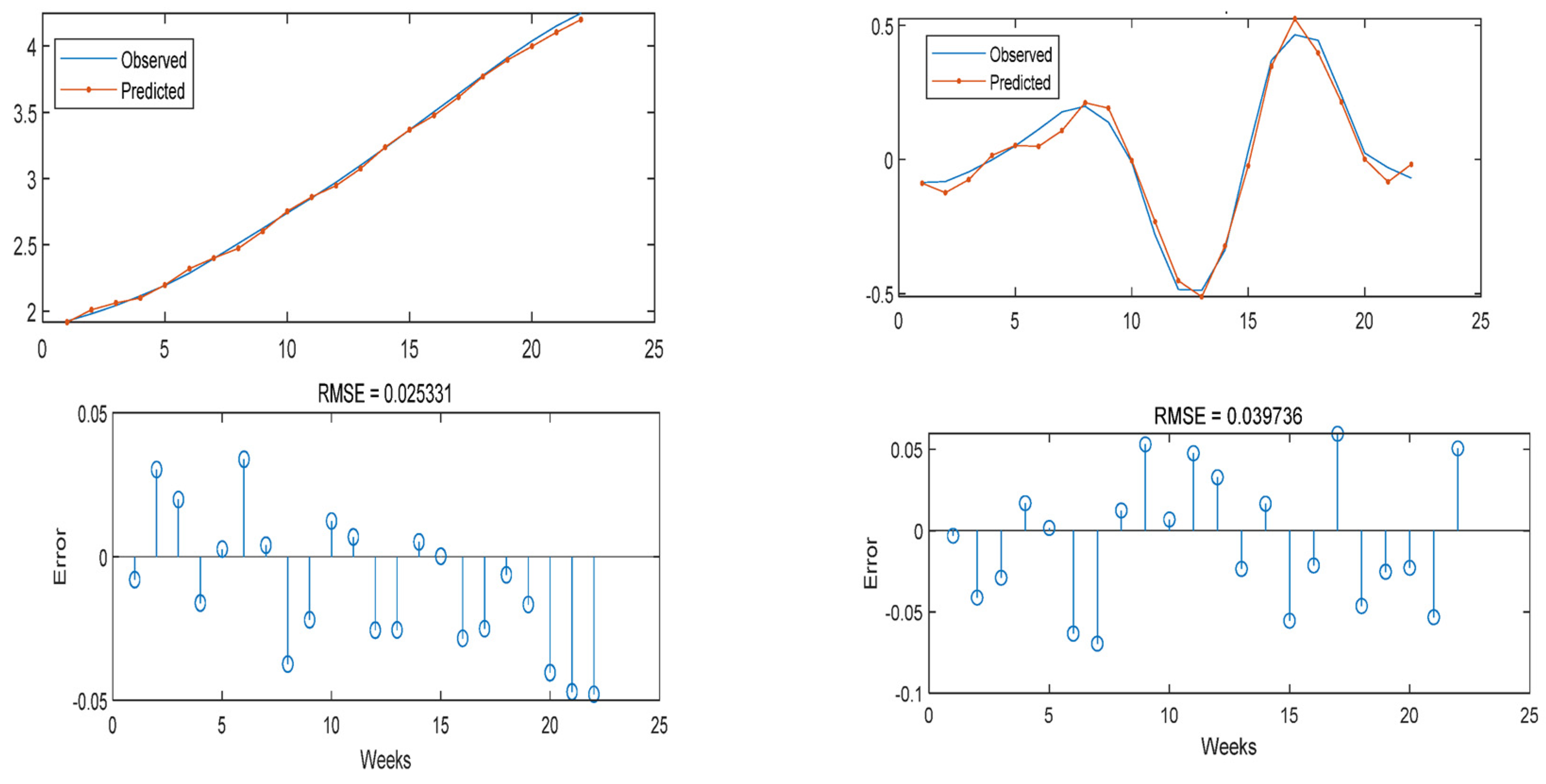
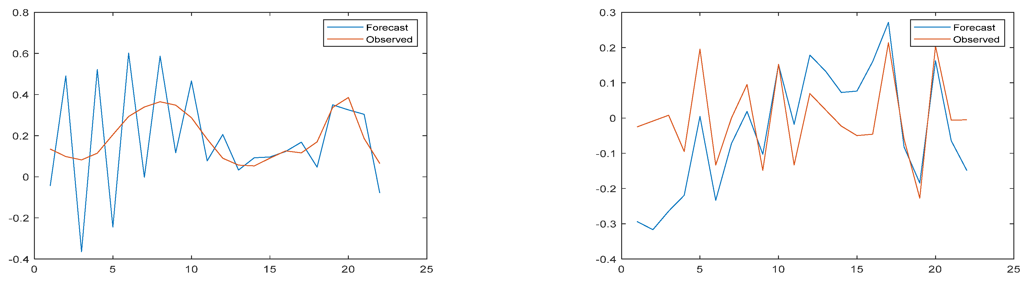
Prediction results and error images of the ANN-WT-LSTM model for high-frequency and low-frequency parts of the Do verification set.
Figure 9.
Prediction results and error images of the ANN-WT-LSTM model for high-frequency and low-frequency parts of the Do verification set.

Figure 10.
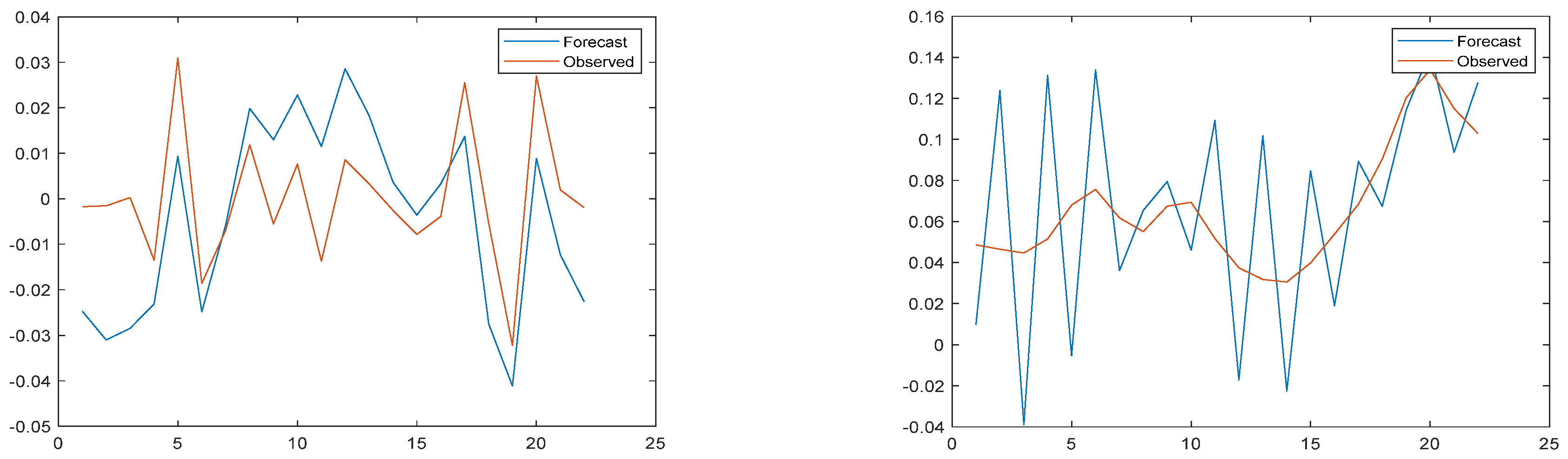
Prediction results and error images of the ANN-WT-LSTM model for high-frequency and low-frequency parts of the CODMN verification set.
Figure 10.
Prediction results and error images of the ANN-WT-LSTM model for high-frequency and low-frequency parts of the CODMN verification set.

Figure 11.
Prediction results and error images of the ANN-WT-LSTM model for high-frequency and low-frequency parts of the TP verification set.
Figure 11.
Prediction results and error images of the ANN-WT-LSTM model for high-frequency and low-frequency parts of the TP verification set.

Figure 12.
Prediction results and error images of the ANN-WT-LSTM model for high-frequency and low-frequency parts of the NH3-N verification set.
Figure 12.
Prediction results and error images of the ANN-WT-LSTM model for high-frequency and low-frequency parts of the NH3-N verification set.

Figure 13.
Prediction results of the ANN-LSTM model on the DO test set and comparison with the original image.
Figure 13.
Prediction results of the ANN-LSTM model on the DO test set and comparison with the original image.

Figure 14.
Prediction results of the ANN-LSTM model on the CODMn test set and comparison with the original image.
Figure 14.
Prediction results of the ANN-LSTM model on the CODMn test set and comparison with the original image.

Figure 15.
Prediction results of the ANN-LSTM model on the TP test set and comparison with the original image.
Figure 15.
Prediction results of the ANN-LSTM model on the TP test set and comparison with the original image.

Figure 16.
Prediction results of the ANN-LSTM model on the NH3-N test set and comparison with the original image.
Figure 16.
Prediction results of the ANN-LSTM model on the NH3-N test set and comparison with the original image.


Table 1.
Overview of water quality prediction research.
| Water Quality Mechanical Prediction Methods | |||
|---|---|---|---|
| Research Scholars | Research Subjects | Model Name | Model Characteristics |
| Lee et al. (2017) [15] | Environmental Fluid Dynamic Code | The Galing River in Kuantan, Pahang, Malaysia | The Environmental Fluid Dynamic Code (EFDC) model considers the effects of temperature, humidity, radiation, cloud cover, evaporation, wind direction, and wind speed, which makes the simulation results closer to the reality. The water quality (TOC, TN, TP) in the upstream section is significantly improved, and the prediction accuracy can be improved by about 37%; if the sewage from the tributary is at the same location, it will increase by about 77%. A total of five water quality management plans for improving the water quality of the Galing River were evaluated using EFDC. |
| Deus et al. (2013) [16] | Two-dimensional water quality model | The Tucuruí reservoir, Pará, Brazil | The use of CE-QUAL-W2 to model hydrodynamics and water quality can reproduce horizontal and vertical gradients and their temporal changes. The field data of temperature, nitrate, ammonia, phosphorus, total suspended solids (TSS), and dissolved oxygen and chlorophyll a are used to verify the prediction effect of the model, and it has been confirmed that it can be used to simulate the response of water quality to the various management schemes of the fish industry. |
| Al-Zubaidi and Wells (2018) [17] | Three-dimensional hydrodynamic model | Lake Chaplain, Washington, DC, USA | The 3D hydrodynamic and water quality model is developed by expanding the 2D fully implicit scheme of CE-QUAL-W2 in three dimensions. The governing equations include a continuity equation, free surface equation, momentum equation, and transport equation, and the momentum and transport equations are solved by the time-splitting technique. The hydrodynamic equation and water quality equation are solved at the same time to realize the feedback between water quality and hydrodynamics. The results showed that the solution of the hydrodynamic equation of the model was very consistent with the field data. |
| Yang et al. (2017) [18] | Finite volume method | Urban Lake in Tianjin, China | The Navier Stokes equation is used to establish a two-dimensional hydraulic model, the finite volume method is used to calculate the parameters of the two-dimensional uncertain eutrophication model, and the Bayesian method is used to correct the model parameters. The model reflects the interaction between nutrients, phytoplankton, and zooplankton. It can be used to simulate the changes of seasonal and regional water quality indicators (DO, NH4+, NO3−, and PO43−), and can calculate hydrodynamic information and eutrophication dynamics with reasonable accuracy (all relative errors are less than 11%). |
| Colton et al. (2022) [19] | Mass balance model | the Laurentian Great Lakes | The model calculates the mass balance and dynamic simulation evaluation of some trace metal loads in the Great Lakes basin, summarizes the loads of the tributaries and connecting channels, and estimates the atmospheric input and sedimentation. Among them, the load of conservative elements (Na and Cl) is used to calibrate the black box method. The mass balance of these elements can be accurately reproduced to 90% in a long-term trend. |
| Wang et al. (2018) [20] | Soft-sensing method based on WASP model | Taihu Lake and Beihai Lake in China | The WASP model is employed as a soft-sensing method and its unknown parameters are estimated by the unscented Kalman filter. The results show that the proposed soft sensing method can describe the changes of relevant water quality indexes (DO, BOD, TN, and Chl_a), and has improved accuracy compared to the nonlinear least square method and traditional trial and error method. |
| Yang et al. (2021) [21] | MIKE 21 FM model | Dongshan Lake in Guangdong Province of China | By using the MIKE 21 FM model and considering different flow arrangements, several model scenarios were established to predict the impact of diversion on selected water quality parameters. The results showed that the inflow and outflow arrangement was the main factor determining the flow field of the whole lake and the change trend of NH3-N, and the increase in flow showed an unequal influence in each region. Wind was also shown to be important for the formation of air circulation and the change of pollutants. |
| Water Quality Non-Mechanical Prediction Method | |||
| Research Scholars | Research Subjects | Model Name | Methods andResults |
| Najafzadeh et al. (2021) [22] | None | SVM, GEP, MTree, EPR, and MARS models | The d-factor of the SVM model was 0.79 for the Kx metric with 95% confidence space. The d-factor value was 0.87 for the Ky metric, which is better than the other models in terms of prediction accuracy. |
| Song et al. (2021) [23] | Haihe River | SWT-ISSA-LSTM | Based on the strong noise immunity of the simultaneous wavelet transform, the simultaneous wavelet transform is used to denoise the dataset, followed by an improved sparrow search algorithm to optimize the hyperparameters of the LSTM. The mean absolute error (MAE) of the model for predicting the water quality of Yongding River was 0.4727, which is much lower than other models. |
| Noori et al. (2013) [24] | Sefidrood River Basin | ROANFIS | The Pearson correlation coefficient (R) and root mean square error of the best-fit ROANFIS model were 0.96 and 7.12, respectively. In the test step of the selected ROANFIS model, the uncertainty analysis showed that the 95% confidence interval and the d-factor were predicted as 94% and 0.83, respectively. |
| Noori et al. (2013) [25] | Sefidrood River Basin | RONNM | The results showed that the best-fit RONNM had a Pearson correlation coefficient (R) and root mean square error of 0.94 and 7.75, respectively. In addition, the accuracy analysis of the model outputs based on the developed difference ratio statistics showed that RONNM was more advantageous. |
| Noori et al. (2015) [26] | Sefidrood River basin | SVM | The percentage of observed data included by the bandwidth of 95% prediction uncertainty (95ppu) and 95% confidence interval (d-factor) was selected for analysis. The results showed that the support vector machine model was more sensitive to the capacity parameter (C) than kernel parameter (gamma) and fault tolerance (epsilon), and it had acceptable uncertainty in BOD5 prediction. |
| Ahmed et al. (2019) [27] | Data from PCRWR | Polynomial regression, random forest, etc. | Multiple linear regression, polynomial regression, random forest, and other machine learning regression models were used to predict WQI separately. The results show that the mean absolute error (MAE) of polynomial regression was 2.7273, which bests the other models in terms of performance. |
| Liu (2019) [28] | Guazhou automatic water quality monitoring station | LSTM | The mean interpolation and Pearson correlation coefficient were first used to preprocess the dataset, followed by LSTM to predict the PH and CODMn metrics. The mean squared error (MSE) of the model was 0.0017 for the DO dataset, which outperformed the ARIMA and SVR models. |
| Hu et al. (2019) [29] | None | LSTM | Linear interpolation and Pearson correlation coefficients were first used to preprocess the dataset, followed by LSTM to predict PH, temperature, and other indicators. The results indicated that in the short-term prediction, the prediction accuracy of PH and water temperature could reach 98.56% and 98.97%, and the prediction time lengths were 0.273 s and 0.257 s, respectively. In the long-term prediction, the prediction accuracy of pH and water temperature could reach 95.76% and 96.88%, respectively. |
| Elias Eze et al. (2021) [30] | South Africa | EEMD-DL-LSTM model | Firstly, EEMD was used to decompose temperature and PH into individual IMF components, and then each IMF component was used as the input of LSTM to train the neural network. The results showed that the average absolute error of this hybrid model was 0.0375, which is much lower than that of the BPNN and DL-LSTM models. |
Table 2.
Descriptive statistics of experimental dataset.
| Index | Minimum Value | Maximum Value | Mean Value | Standard Deviation | Variance | Number of Missing Values |
|---|---|---|---|---|---|---|
| DO | 4.80 | 11.10 | 7.49 | 1.19 | 1.19 | 1 |
| CODMn | 1.10 | 5.30 | 2.64 | 0.74 | 0.74 | 1 |
| TP | 0.00 | 0.19 | 0.09 | 0.03 | 0.03 | 0 |
| NH3-N | 0.02 | 0.95 | 0.29 | 0.17 | 0.17 | 2 |
Table 3.
Correlation coefficients for each dataset.
| Correlation Coefficient | DO | CODMn | TP | NH3-N |
|---|---|---|---|---|
| DO | 1 | −0.024 | −0.201 | −0.136 |
| CODMn | - | 1 | 0.031 | 0.087 |
| TP | - | - | 1 | 0.448 |
| NH3-N | - | - | - | 1 |
Table 4.
Wavelet reconstruction error table for each parameter.
| Parameters | Error Value |
|---|---|
| DO | 9.1 × 10⁻¹⁶ |
| CODMn | 6.75 × 10⁻¹⁶ |
| NH3-N | 8.13 × 10⁻¹⁶ |
| TP | 8.35 × 10⁻¹⁶ |
Table 5.
Parameter settings of ANN-WT-LSTM and traditional LSTM models.
| Model Parameters | ANN-WT-LSTM | ANN-LSTM | |
|---|---|---|---|
| Data Type | cA | cD | Data Interpolated by Artificial Neural Network |
| Number of hidden layer units a | 300 | 300 | 300 |
| Learning rate (%) b | 0.003 | 0.003 | 0.001 |
| Forgetting rate (%) c | 0.2 | 0.2 | 0.2 |
| Gradient threshold d | 1 | 1 | 1 |
| Number of iterations e | 250 | 250 | 250 |
| Batch size f | 32 | 32 | 32 |
a NAR neural network parameter settings: autoregressive coefficient lag = 3, number of hidden layer units = 300. b Set to reduce the learning rate by multiplying by a factor of 0.2 after 125 rounds of training. c BPNN parameter settings: number of hidden layer units = 300 and number of iterations = 250; d SSA-LSTM parameters: dim is 4, the range of learning rate is (0.001,1), the range of the maximum number of iterations is (10,500), number of sparrows = 5, warning value ST = 0.6, proportion of discoverers PD = 0.6, proportion of sparrows aware of danger SD = 0.2, and population size = 5; e ISSA-BPNN: based on the fact that the sparrow search algorithm tends to fall into a local optimum, a tent mapping was used to initialize the population for the sparrow search algorithm. f The parameters were set as follows: lower boundary (lb) of the weight threshold is −5 and upper boundary (ub) of the weight queue is 5.
Table 6.
Analysis and comparison of ANN-WT-LSTM model and other models on dataset.
| Parameter | DO | CODMn | TP | NH3-N | |
|---|---|---|---|---|---|
| Model | |||||
| ANN-W-LSTM | MSE | 8.3 × 10⁻²⁵ | 0.0006 | 0.00068 | 0.006 |
| RMSE | 9.13 × 10⁻¹³ | 0.024 | 0.026 | 0.0776 | |
| MAPE | 5.65 × 10⁻¹³ | 0.021 | 0.243 | 0.0232 | |
| MAE | 4.39 × 10⁻¹² | 0.014 | 0.014 | 0.011 | |
| ANN-LSTM | MSE | 2.536 | 0.539 | 0.0009 | 0.03 |
| RMSE | 1.5927 | 0.7341 | 0.03 | 0.232 | |
| MAPE | 0.106 | 0.178 | 0.355 | 2.88 | |
| MAE | 0.94 | 0.52 | 0.02 | 0.181 | |
| NAR | MSE | 2.2889 | 1.1353 | 0.0012 | 1.945 |
| RMSE | 1.5129 | 1.0655 | 0.0345 | 1.395 | |
| MAPE | 0.1489 | 0.2593 | 0.563 | 13.639 | |
| MAE | 1.2417 | 0.813 | 0.026 | 1.149 | |
| ARIMA | MSE | 3.1659 | 0.9277 | 0.0013 | 0.0297 |
| RMSE | 1.7793 | 0.9632 | 0.0359 | 0.1723 | |
| MAPE | 0.1711 | 0.1959 | 0.6434 | 2.1502 | |
| MAE | 1.4999 | 0.7009 | 0.0306 | 0.1601 | |
| MLPNN | MSE | 2.7947 | 0.728 | 0.0011 | 0.015 |
| RMSE | 1.67 | 0.853 | 0.033 | 0.122 | |
| MAPE | 1.403 | 0.698 | 0.29 | 0.11 | |
| MAE | 0.159 | 0.267 | 0.589 | 1.27 | |
| CNN-LSTM | MSE | 2.35 | 0.25 | 0.018 | 0.008 |
| RMSE | 1.53 | 0.5 | 0.134 | 0.09 | |
| MAPE | 0.015 | 0.15 | 0.96 | 0.28 | |
| MAE | 1.17 | 0.4 | 0.11 | 0.02 | |
| BPNN | MSE | 0.27 | 0.126 | 0.2 | 0.07 |
| RMSE | 0.52 | 0.35 | 0.45 | 0.26 | |
| MAPE | 3.87 | 1.59 | 1.22 | 1.11 | |
| MAE | 0.42 | 0.29 | 0.41 | 0.22 | |
| SSA-LSTM | MSE | 1.4 | 0.27 | 0.02 | 0;009 |
| RMSE | 1.18 | 0.52 | 0.14 | 0.095 | |
| MAPE | 0.14 | 0.16 | 0.12 | 0.44 | |
| MAE | 1.16 | 0.42 | 0.11 | 0.024 | |
| ISSA-BPNN | MSE | 0.14 | 0.062 | 0.12 | 0.05 |
| RMSE | 0.37 | 0.25 | 0.35 | 0.22 | |
| MAPE | 5.13 | 1.3 | 0.92 | 2 | |
| MAE | 0.29 | 0.2 | 0.31 | 0.18 | |
| SSA-BPNN | MSE | 0.15 | 0.063 | 0.13 | 0.1 |
| RMSE | 0.38 | 0.251 | 0.36 | 0.32 | |
| MAPE | 1.73 | 0.77 | 0.98 | 1.86 | |
| MAE | 0.29 | 0.2 | 0.32 | 0.19 | |
| DWT-CNN-LSTM | MSE | 0.24 | 0.04 | 0.002 | 0.03 |
| RMSE | 0.49 | 0.2 | 0.045 | 0.173 | |
| MAPE | 0.05 | 0.05 | 0.5 | 1.62 | |
| MAE | 0.39 | 0.15 | 0.043 | 0.13 | |
| EMD-LSTM | MSE | 1.67 | 0.07 | 0.035 | 0.022 |
| RMSE | 1.3 | 0.26 | 0.19 | 0.15 | |
| MAPE | 0.14 | 0.06 | 0.62 | 1.96 | |
| MAE | 1.1 | 0.2 | 0.13 | 0.12 | |
| EEMD-LSTM | MSE | 1.12 | 0.07 | 0.037 | 0.016 |
| RMSE | 1.06 | 0.26 | 0.192 | 0.126 | |
| MAPE | 0.11 | 0.07 | 0.62 | 1.64 | |
| MAE | 0.89 | 0.20 | 0.13 | 0.105 |
Publisher’s Note: MDPI stays neutral with regard to jurisdictional claims in published maps and institutional affiliations. |
© 2022 by the authors. Licensee MDPI, Basel, Switzerland. This article is an open access article distributed under the terms and conditions of the Creative Commons Attribution (CC BY) license (https://creativecommons.org/licenses/by/4.0/).
Share and Cite
MDPI and ACS Style
Wu, J.; Wang, Z. A Hybrid Model for Water Quality Prediction Based on an Artificial Neural Network, Wavelet Transform, and Long Short-Term Memory. Water 2022, 14, 610. https://doi.org/10.3390/w14040610
AMA Style
Wu J, Wang Z. A Hybrid Model for Water Quality Prediction Based on an Artificial Neural Network, Wavelet Transform, and Long Short-Term Memory. Water. 2022; 14(4):610. https://doi.org/10.3390/w14040610
Chicago/Turabian StyleWu, Junhao, and Zhaocai Wang. 2022. "A Hybrid Model for Water Quality Prediction Based on an Artificial Neural Network, Wavelet Transform, and Long Short-Term Memory" Water 14, no. 4: 610. https://doi.org/10.3390/w14040610
Note that from the first issue of 2016, this journal uses article numbers instead of page numbers. See further details here.