Development of Deep Learning Models to Improve the Accuracy of Water Levels Time Series Prediction through Multivariate Hydrological Data

Abstract

Since predicting rapidly fluctuating water levels is very important in water resource engineering, Long Short-Term Memory (LSTM) and Gated Recurrent Unit (GRU) were used to evaluate water-level-prediction accuracy at Hangang Bridge Station in Han River, South Korea, where seasonal fluctuations were large and rapidly changing water levels were observed. The hydrological data input to each model were collected from the Water Resources Management Information System (WAMIS) at the Hangang Bridge Station, and the meteorological data were provided by the Seoul Observatory of the Meteorological Administration. For high-accuracy high-water-level prediction, the correlation between water level and collected hydrological and meteorological data was analyzed and input into the models to determine the priority of the data to be trained. Multivariate input data were created by combining daily flow rate (DFR), daily vapor pressure (DVP), daily dew-point temperature (DDPT), and 1-hour-max precipitation (1HP) data, which are highly correlated with the water level. It was possible to predict improved high water levels through the training of multivariate input data of LSTM and GRU. In the prediction of water-level data with rapid temporal fluctuations in the Hangang Bridge Station, the accuracy of GRU’s predicted water-level data was much better in most multivariate training than that of LSTM. When multivariate training data with a large correlation with the water level were used by the GRU, the prediction results with higher accuracy ($R^2=0.7480–0.8318$; $NSE=0.7524–0.7965$; $MRPE=0.0807–0.0895$) were obtained than those of water-level prediction results by univariate training.

1. Introduction

South Korea is a monsoon climate where 60–70% of annual average precipitation is concentrated from June to September. Therefore, flood damage in summer is concentrated, and drought damage is caused in spring, making it difficult to manage water resources [1]. In the case of urban rivers, the watersheds are covered with impervious layers, resulting in a series of urban flood damage due to the rapid increase in direct runoff caused by heavy rain, so accurate flood-prediction technology is needed and is essential to prevent flood disasters [2]. Therefore, local heavy rains caused by climate change frequently cause extreme flood damage around urban rivers, so techniques for accurately predicting the high water level or high flow rate of urban rivers are essential [3].

In the past, flow rates and water levels were calculated in the event of a flood, using the physical numerical model that used the Computational Fluid Dynamics (CFD) method, but there were limitations in obtaining sufficiently reliable results in terms of time, cost, and accuracy of the prediction model [4]. Therefore, in the field of water resource engineering, as a way to replace the existing physical models and improve the prediction accuracy of hydrological quantities, researchers have developed data-driven models that can predict hydrological quantities only through the analysis of input data.

As a traditional data-driven model, the Auto-Regressive Integrated Moving Average (ARIMA) model was used to analyze linear time-series data, such as prediction of monthly mean water levels to perform water-level prediction [5]. In the case of the ARIMA model, the prediction accuracy of the linear hydrological data was calculated with appropriate prediction accuracy, whereas, in the case of hydrological time-series data with nonlinear characteristics, the prediction accuracy of the nonlinear hydrological data was deteriorated [6]. In addition, the ARIMA model was mainly used to predict time-series groundwater levels [7]. However, there was a limitation in that the correlation between hydrological variables, including rainfall and groundwater level, could not be properly considered [8].

In the case of the Fuzzy and Neural Network (NN) system, it was effectively used for reservoir operation [9]. In addition, the Adaptive Network-Based Fuzzy Inference System (ANFIS) was used to predict the water level with the high reliability of the reservoir [10]. However, in the case of Neuro-Fuzzy model, in time-series groundwater prediction with nonlinear characteristics, the prediction accuracy of the model significantly decreased as the prediction period increased [8].

Accordingly, studies on data-driven models based on the Fourth Industrial Revolution technology that can overcome and replace the limitations of existing physical models are currently being actively studied [4]. A typical data-driven model is a Deep Neural Network (DNN) model, and in contrast to the calculations of numerical solution according to the initial and boundary conditions of the governing equation, accurate prediction results can be obtained by repeatedly training input value data and calculating parameters of the data-driven model. Recently, research on the prediction of time-series data, such as the flow rate, water level, and flow velocity of rivers and reservoirs in the field of water resource engineering, using the DNN model, is being actively conducted [11,12,13,14,15,16,17,18,19].

In the past five years, DNN models have been used to predict various hydrological quantities, such as water level, flow rate, and precipitation in water resource engineering. However, most studies have mainly studied predicting water levels that change smoothly over the entire time or predicting flow rates in rivers and reservoirs with little temporal flow changes. Especially, DNN was widely used to predict groundwater levels [20], water levels in the stream [21,22,23], wetlands [24,25], and reservoirs [26,27,28]. However, most of these studies on water-level predictions correspond to cases where the water-level change according to temporal changes is mild, and the accuracy of the prediction results could not be guaranteed if the water-level change changes rapidly [4]. Therefore, the studies on predicting water levels with high temporal variability in the rivers were recognized as limitations of the DNN models and were rarely conducted, as compared to other research areas. It is essential to predict the exact amount of hydrological quantities in the river due to torrential rains or typhoons caused by climate change and urbanization, but it was difficult to trust the prediction results of DNN models under high-water-level or high-flow-rate conditions. Nevertheless, there was a study to predict river flow rates with high accuracy by providing guidelines for input training data [4]. In addition, real-time groundwater-level prediction [29], extreme water-level prediction by highest tide [30,31], and real-time urban-river-flood-level prediction, using various DNN models, have been effectively performed recently [32]. However, until recently, there were not many studies to improve the accuracy of predicting water levels with very high temporal variability. This study attempted to improve the prediction result of river water levels with high temporal fluctuations by diversifying the input data by analyzing the correlation of input data, using DNN models.

The main purpose of this study was to establish the multivariate training models that can accurately predict daily water-level data under high-water-level conditions among rapidly changing hydrological quantities by selecting DNN models that are effective in predicting time-series hydrological data. Previous DNN studies in the field of water resource engineering focused on predicting gentle water level changes, but this study aimed to predict high-water-level changes in a river that has very severe temporal fluctuations. In addition, most previous studies used only univariate water-level data as input data to predict the water level, so there was a limit to predicting the high water levels that rise dramatically by season.

The purpose of this study is as follows. First, in order to predict the time-series water levels that change rapidly over time, hydrological data and meteorological data that have a large correlation with the water levels will be selected. Second, hydrological data or meteorological data with a large correlation with the water level will be selected, and DNN models suitable for predicting hydrological time series data (i.e., water level and flow rate) will be selected. Third, the accuracy of the water-level prediction will be analyzed by using hydrological data or meteorological data, which have a large correlation with the water level, as input data of the DNN model. Finally, the DNN models will be proposed with improved accuracy of water-level prediction according to multivariate input data effective in predicting time-series levels that change rapidly from low to high levels. Therefore, it is expected that the accuracy of predicting low and high water levels will be improved through the types and numbers of multivariate training data.

2. Methods

2.1. Applied DNN Models

Among the DNN models that can be effectively used for time-series data analysis, in this study, Long Short-Term Memory (LSTM) and Gated Recurrent Unit (GRU) were selected and used as Recurrent Neural Network (RNN) models that can be appropriately applied to past hydrological time-series data [4].

2.1.1. Long Short-Term Memory (LSTM)

LSTM is a sequential data model that improves the long-term memory loss problem of Simple RNN [4,33]. As shown in Figure 1, LSTM consists of a forget gate, an input gate, and an output gate. The key to LSTM is to have a cell state. The horizontal line from $c_{t-1}$ to $c_t$ located at the top of Figure 1 is called the cell state that penetrates the entire time-series data through a simple linear operation. Because of this structure, time-series information continues to be sent to the next time step without memory loss.

$$f_t=\mathsf{\sigma }\left(W_f·\left[h_{t-1}, x_t\right]+b_f\right)$$

(1)

$$i_t=\mathsf{\sigma }\left(W_i·\left[h_{t-1}, x_t\right]+b_i\right)$$

(2)

$${\overline{c}}_t=\tanh \left(W_c·\left[h_{t-1}, x_t\right]+b_c\right)$$

(3)

$$c_t=f_t c_{t-1}+i_t {\overline{c}}_t$$

(4)

$$o_t=\mathsf{\sigma }\left(W_o·\left[h_{t-1}, x_t\right]+b_o\right)$$

(5)

$$h_t={\mathrm{o}}_t\tanh \left(c_t\right)$$

(6)

where $f_t$, $i_t$, and $o_t$ are the forget, input, and output gates at time, $t$, respectively; $W_f$, $W_i$, and $W_o$ are weights mapped to hidden layers for forget, input, and output gates; $b_f$, $b_i$, and $b_o$ are bias vectors; $h$ is layer; $\mathsf{\sigma }\left(·\right)$ is an activation function; $\tanh \left(·\right)$ is hyperbolic tangent function; $c_{t-1}$ and $c_t$ are the cell states of the previous time step and the next time step.

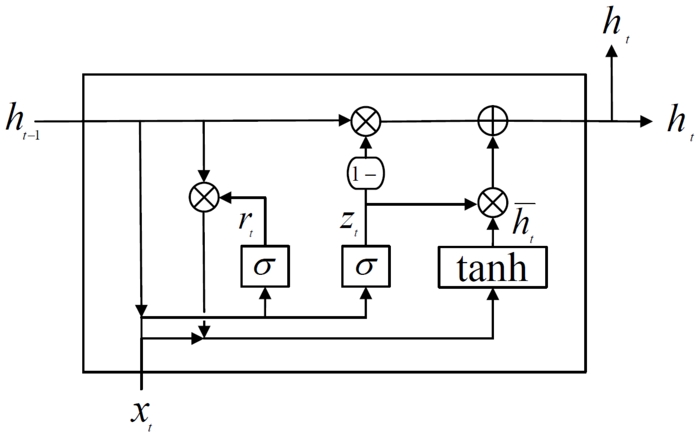
2.1.2. Gated Recurrent Unit (GRU)

GRU plays a similar role as LSTM, but it is computationally efficient because it consists of a simpler structure. This reduced the calculation of cell state used by the LSTM. GRU is a simplified form of three gates of LSTM. As shown in Figure 2, the input gate and forget gate are combined and simplified into an update gate [4,34]. There are only two types of GRU: an update gate, a reset gate, and a removed cell state. GRU has two activation functions and one tanh function. Therefore, GRU has fewer parameters and faster training speed than LSTM, but long-term memory, such as LSTM, is possible.

$$r_t=\mathsf{\sigma }\left(W_r·\left[h_{t-1}, x_t\right]+b_r\right)$$

(7)

$$z_t=\mathsf{\sigma }\left(W_z·\left[h_{t-1}, x_t\right]+b_z\right)$$

(8)

$${\overline{h}}_t=\tanh \left(W·\left[h_{t-1}, x_t\right]+b\right)$$

(9)

$$h_t=\left(1-z_t\right)h_{t-1}+z_t {\overline{h}}_t$$

(10)

where $r$ and $z$ are the reset and update gates, respectively. Reset gate aims to reset past data and outputs a value between 0 and 1, which is the value of how much past data will be reset through the activation function. The update gate determines the rate of past and present information updates and the output value, $z_t$, determines the amount of data to be exported at this point in time; $1-z_t$ is the amount of data to be forgotten.

2.2. Model Performance Indicators

Equations (11)–(17) were used as evaluation criteria for the RNN models to evaluate the performance and accuracy of the models. The closer the Mean Absolute Error (MAE), Mean Square Error (MSE), Root Mean Square Error (RMSE), and Mean Relative Peak Error (MRPE) are to 0, the better the performance of the model. As the Nash–Sutcliffe model Efficiency coefficient (NSE) and the determination coefficient ($R^2$) are close to 1, the performance of the model is improved.

(1)

Mean Absolute Error (MAE)

MAE measures the average magnitude of the error in the prediction set without considering the direction. This is the mean for the test sample for absolute differences between predictions and actual observations where all individual differences have the same weight [4,35]

$$MAE=\frac{1}{N}{\displaystyle \sum }_{i=1}^N\left|x_i-y_i\right|$$

(11)

where $x_i$ is the observed values of the variables, $y_i$ is the predicted values, and $N$ is the number of data.

(2)

Mean Squared Error (MSE)

MSE measures the mean of the squares of the errors, that is, the mean squared difference between the predictions and the actual observations [4,35].

$$MSE=\frac{1}{N}{\displaystyle \sum }_{i=1}^N{\left(x_i-y_i\right)}^2$$

(12)

(3)

Root Mean Squared Error (RMSE)

RMSE is a quadratic scoring rule that also measures the average magnitude of an error. It is the square root of the average of squared differences between predictions and actual observations [4,35,36,37].

$$RMSE=\sqrt{\frac{{{\displaystyle \sum }}_{i=1}^N{\left(x_i-y_i\right)}^2}{N}}$$

(13)

(4)

Coefficient of determination ($R^2$)

The coefficient of determination, $R^2$, is a measure of the goodness of fit of the statistical model [4,35,38,39].

$$R^2=1-\frac{{{\displaystyle \sum }}_{i=1}^N{\left(x_i-{\widehat{y}}_i\right)}^2}{{{\displaystyle \sum }}_{i=1}^N{\left(x_i-\overline{x}\right)}^2}$$

(14)

where ${\widehat{y}}_i$ are the predicted values from a statistical model, and $\overline{x}$ is the mean of observed values of the variables.

(5)

Nash–Sutcliffe model efficiency coefficient (NSE)

NSE is used to quantify how well model simulations can predict the outcome variables [4,35,36,38,39].

$$NSE=1-\frac{{{\displaystyle \sum }}_{i=1}^N{\left(x_i-y_i\right)}^2}{{{\displaystyle \sum }}_{i=1}^N{\left(x_i-\overline{x}\right)}^2}$$

(15)

As shown in

Table 1. Performance ratings for adopted statistics.

Performance Rating	${\mathit{R}}^2$	$\mathit{N}\mathit{S}\mathit{E}$
Very good	$0.75<R^2\le 1.00$	$0.75<NSE \le 1.00$
Good	$0.65<R^2\le 0.75$	$0.65<NSE \le 0.75$
Satisfactory	$0.50<R^2\le 0.65$	$0.50<NSE \le 0.65$
Unsatisfactory	$R^2\le 0.50$	$NSE \le 0.50$

, it is not appropriate to adopt model results if $R^2$ and $NSE$ are less than 0.5; model adoption is possible if $R^2$ and $NSE$ are greater than 0.5 and less than 0.65; model adoption is good if $R^2$ and $NSE$ are greater than 0.65 and less than 0.75; and if $R^2$ and $NSE$ are over 0.75, it is very good to adopt a model [4,19,35,38,40].

(6)

Mean Relative Peak Error (MRPE)

The Relative Peak Error (RPE) for each i-th event and MRPE are used to evaluate the prediction accuracy for peak values:

$$RP{E}_i=\frac{y_{pi}-x_{pi}}{x_{pi}}$$

(16)

$$MRPE=\frac{{{\displaystyle \sum }}_{i=1}^N\left|RP{E}_i\right|}{M}$$

(17)

where $y_{pi}$ are the predicted peak values for each i-th event, $x_{pi}$ are the observed peak values for each i-th event, and $M$ is the number of events. It means that, the closer the MRPE is to zero, the better the peak values of the model are predicted [41].

2.3. Application of Models

As shown in Figure 3, in this study, a flowchart for predicting time-series water levels by using LSTM and GRU models was presented. This study attempted to compare the accuracy of rapidly varying water-level prediction and the performance of models, using LSTM and GRU models. Data input and output to time-series models basically use water levels. However, since the water-level data alone have limitations in accurately predicting the rapidly changing water level, this study attempted to analyze the accuracy of the predicted water levels by using hydrological data (i.e., flow rate, temperature, vapor pressure, and precipitation) that are close to correlation with the water level as input data.

Considering the number of hydrological input data and the correlation between the data, it is intended to overcome the limitation of not accurately providing rapidly changing water levels, as in previous research cases, by using it as a single hydrological time-series input data. Therefore, the purpose of this study was to accurately predict the water level by using not only the water level but also time-series hydrological data, which are multivariate data, as additional input data.

3. Study Area and Data

3.1. Study Area

The Han River in the urbanized Han River basin was selected (Figure 4). The Han River basin is located in the central part of the Korean Peninsula and spans 36°30′ to 38°55′ N latitude, 126°24′ to 129°02′ E longitude. As shown in

Table 2. Summary of site characteristics.

Length of River (km)	Basin Area $\left({\mathrm{km}}^2\right)$	Mean Rainfall (mm/Year)	Mean Water Level $(\mathrm{EL}.\mathrm{m})$	Mean Streamflow $\left({\mathrm{m}}^3/\mathrm{s}\right)$
494.44	25,953.60	1313.42	0.91	355.97

EL.: Elevation

, the Han River is the largest river in South Korea, with a basin area of 25,953.60 ${\mathrm{km}}^2$, a total length of 494.44 km, an average width of 72.35 km, and a shape coefficient of 0.146. The Han River basin is a multi-form basin mixed with dendritic and facsimile forms. Historically, the Han River was destroyed as the channel was changed due to the urbanization of the Han River basin [4,42]. In 2003, the primary land was 5.4% agricultural land, 25.6% forest, 8.8% river, 39.4% vacant land, 2.5% park land, and 18.3% urban land [4,42]. Table 2 summarizes the channel characteristics. The channelized reach with an average river width of 1300 m has an average slope of 0.0016% on the downstream distance of the Han River basin [4,43,44].

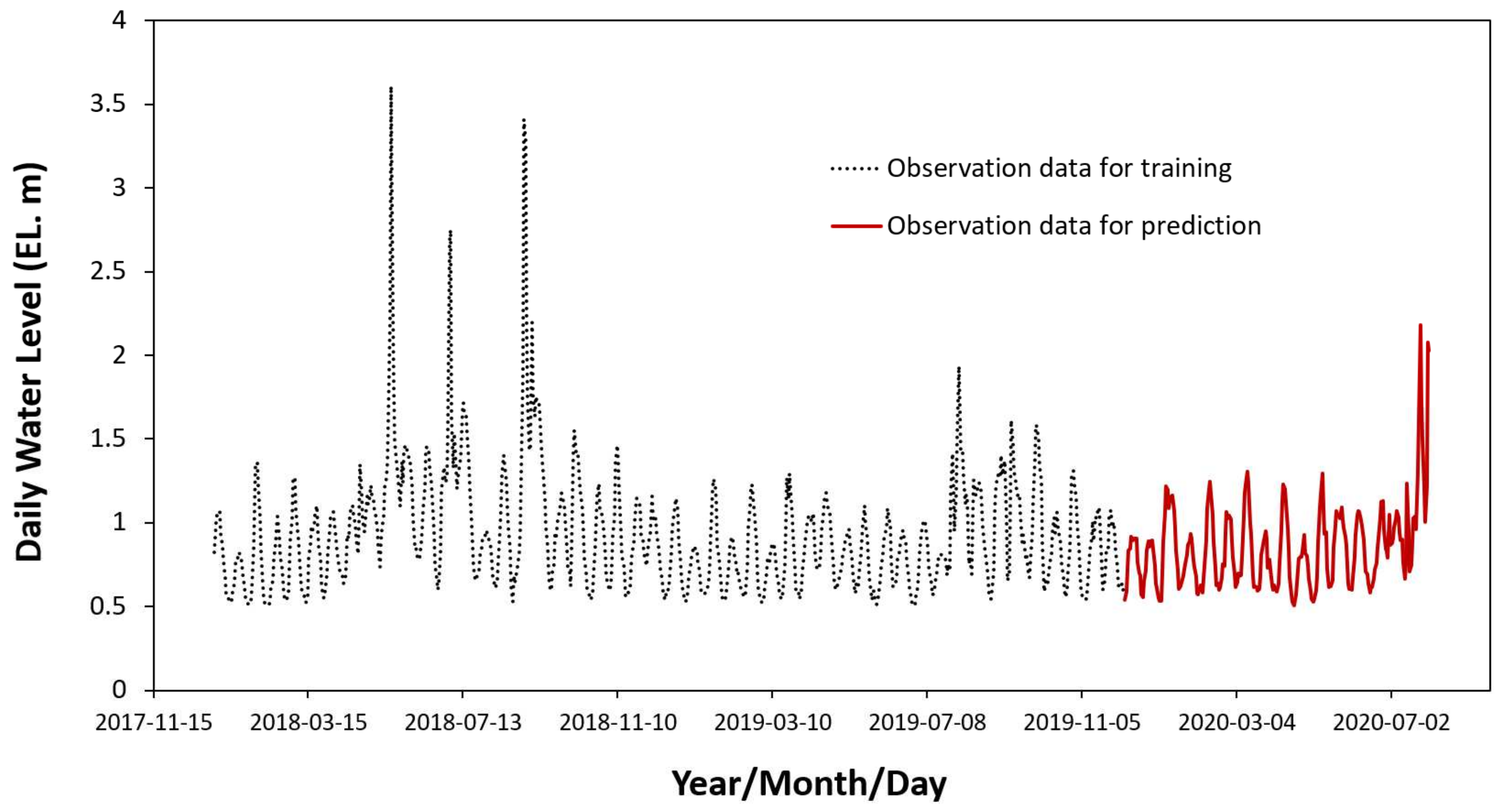
3.2. Hydrologic Data

In this study, the hydrological data of Hangang Bridge Station observed by the Ministry of Environment, Korea, were used (Figure 4). In order to utilize weather data, the Korea Meteorological Administration (KMA) observatory closest to Hangang Bridge Station used data from the Seoul Observatory (Figure 4). The flow rate and water-level data at the flow-measuring station were obtained by using data from the Water Resources Management Information System (WAMIS) website of the Ministry of Environment [45]. Meteorological data from the Seoul observatory were obtained through the website of the KMA National Climate Data Center [46]. The average annual precipitation from 2010 to 2019 was 1313.42 mm, and based on the precipitation data provided on the Meteorological Administration website [46], 60% of the precipitation fell during the monsoon season between July and September. Therefore, since seasonal rainfall is concentrated in summer, the runoff also increases rapidly during this period.

(1)

Daily water level

In this study, the longer the data of the learning data, the better the prediction results of the model generally, so the total length of the data used for learning and prediction was 2 years and 7 months, and the relatively short data were used to verify the deep learning models. As shown in

Table 3. Statistical characteristics of water levels at the Hangang Bridge Station (period: 2018–2020).

Minimum Water Level $(\mathrm{EL}.\mathrm{m})$	Maximum Water Level $(\mathrm{EL}.\mathrm{m})$	Average Water Level $(\mathrm{EL}.\mathrm{m})$	Standard Deviation of Water Level $(\mathrm{EL}.\mathrm{m})$	Coefficient of Flow Fluctuation (CFF)
0.504	3.606	0.915	0.336	70.32

and Figure 5, the observed average water levels from the Hangang Bridge Station were based on real-time observed data from 1 January 2018 to 31 July 2020. In Figure 5, training and prediction data were selected for the purpose of evaluating the performance of DNN models that can sufficiently predict rapid water-level fluctuations occurring between June and July 2020 by learning rapid water-level fluctuations during the rainy season in 2018. In order to analyze the characteristics of water levels, the average, the minimum, and the maximum water levels were statistically analyzed as shown in Table 3. Prior to the construction of a multipurpose dam on the Han River, the Coefficient of Flow Fluctuation (CFF) was 390: CFF is defined as the ratio of the annual maximum flow rate to the annual minimum flow rate [4,48]. Large-scale multipurpose dams were constructed at upstream: CFF was drastically lowered to 70.32 after constructing a multipurpose dam for flood control and securing water supply.

As shown in Figure 5, the selected daily average time-series water-level data were divided into data for learning and prediction of the models. In the case of rapidly changing hydrological time-series data, using previous research results [4], the best accuracy could be obtained if the optimal length of learning data and predictive data were selected as 74.9% and 25.1%, respectively, from the length of all time-series data. Therefore, as shown in Figure 5, data with black dotted lines were used as learning data for the models, and solid-red-line data were used as forecast data for the models and used to evaluate the accuracy of the models.

(2)

Hydrological and meteorological data

In order to analyze the characteristics of meteorological and hydrological data, the average (Ave), maximum (Max), minimum (Min), and standard deviation (SD) values of the data were divided into training and predictive data and presented as shown in

Table 4. Characteristics of hydrological and meteorological data.

Variable	Training Data				Prediction Data				Train/Predict
	Ave	Max	Min	SD	Ave	Max	Min	SD	Ave	Max	Min	SD
Daily Water Level (EL.m)	1.02	3.61	0.51	0.43	0.86	2.18	0.50	0.25	0.84	0.60	0.98	0.58
Daily Flow Rate (m3/s)	451.66	5752.81	64.65	640.31	275.33	2923.08	59.25	240.95	0.61	0.51	0.92	0.38
Daily Vapor Pressure (hPa)	11.78	31.60	0.70	8.24	10.58	31.80	0.80	7.84	0.90	1.01	1.14	0.95
Daily Dew-Point Temperature (°C)	5.21	25.00	−27.60	12.45	3.59	25.00	−25.80	11.98	0.69	1.00	0.94	0.96
1-Hour-Max Precipitation (mm)	1.35	43.50	0.00	4.65	0.84	29.40	0.00	3.19	0.62	0.68	0.00	0.69
Precipitation Duration (hour)	2.48	24.00	0.00	4.85	2.34	24.00	0.00	4.70	0.94	1.00	0.00	0.97
Daily Precipitation (mm)	3.76	96.50	0.00	12.42	2.60	103.10	0.00	9.14	0.69	1.07	0.00	0.74
Daily Temperature (°C)	14.05	33.70	−14.80	11.09	12.69	31.60	−10.50	10.16	0.90	0.94	0.72	0.92
10-Minute-Max Precipitation (mm)	0.59	25.50	0.00	2.11	0.34	11.90	0.00	1.24	0.58	0.47	0.00	0.59

Ave, average; Max, maximum; Min, minimum; SD, standard deviation; Train/Predict: the ratio of prediction data to training data.

. In addition, for each dataset, the ratios of predictive data for training data (Train/predict) were presented. Except for the daily water level (DWL), the shaded prediction data presented in Table 4 were not actually used as prediction data for deep learning models in this study. However, they were included in the prediction data for characteristic analysis between the two datasets divided into prediction data and training data.

As shown in Table 4, when calculating the ratio of the maximum predicted data to learning data through statistical analysis, DWL was 0.60, daily flow rate (DFR) was 0.51, daily vapor pressure (DVP) was 1.01, daily dew-point temperature (DDPT) was 1.00, and 1-hour-max precipitation (1HP) was 0.68, respectively. In addition, the ratio of standard deviation representing the distribution of data was 0.58 for DWL, 0.38 for DFR, 0.95 for DVP, 0.96 for DDPT, and 0.69 for 1HP, respectively. Therefore, it was found that DWL, DFR, and 1HP were smaller than the maximum values of the prediction data than those of the training data, and the ratio of maximum values was almost no difference in DVP and DDPT. The ratio of standard deviation representing the distribution range of data was 0.38 in DFR, which was the narrowest distribution range of prediction data than training data, and the prediction data gradually increased to the distribution range of training data in the order of DWL, 1HP, DVP, and DDPT.

As shown in

Table 5. Correlation between hydrological and meteorological data.

Variable	Daily Water Level (EL.m)	Daily Flow Rate (m3/s)	Daily Vapor Pressure (hPa)	Daily Dew-Point Temperature (°C)	1-Hour-Max Precipitation (mm)
Daily Water Level (EL.m)	1.0000	0.7731	0.3622	0.3444	0.3305
Daily Flow Rate (m3/s)	0.7731	1.0000	0.3397	0.3112	0.3563
Daily Vapor Pressure (hPa)	0.3622	0.3397	1.0000	0.9465	0.3746
Daily Dew-Point Temperature (°C)	0.3444	0.3112	0.9465	1.0000	0.3140
1-Hour-Max Precipitation (mm)	0.3305	0.3563	0.3746	0.3140	1.0000
Precipitation Duration (hour)	0.2271	0.2641	0.2934	0.2800	0.5210
Daily Precipitation (mm)	0.2993	0.3203	0.3118	0.2741	0.8263
Daily Temperature (°C)	0.3038	0.2656	0.8964	0.9509	0.2198
10-Minute-Max Precipitation (mm)	0.3226	0.3470	0.3836	0.3160	0.9522

, in order to select appropriate input data for DWL prediction, the correlation between meteorological and hydrological data was analyzed. First, the hydrological variables with the greatest correlation with the daily water level were analyzed. The hydrological variable with the greatest correlation with the daily water level to be predicted was the DFR, which was 0.7731, which had a very high correlation between the two data. However, unexpectedly, the correlation coefficient of daily precipitation (DP) was 0.2993, which was judged to have little direct correlation with the daily water level. As shown in Figure 4, the data from the Seoul Observatory of the Meteorological Administration were used for the provided precipitation data. The Seoul Observatory of the Meteorological Administration is about 6 km away from the Hangang Bridge Station, the prediction point of the model, and the Namsan Mountain is located in the middle of the two points, which may cause heterogeneity in weather phenomena, due to topographical factors. Among the collected meteorological data, the data that can be used through correlation analysis with water level are DVP and DDPT. The daily vapor pressure had a correlation coefficient of 0.3622 with the water level, and daily dew-point temperature had a correlation coefficient of 0.3444 with the water level, respectively. Although both data do not have a large correlation with the water level, the predictive performance analysis of LSTM and GRU models was conducted by using multivariate input data (i.e., daily vapor pressure and daily dew-point temperature). Second, the correlation between hydrological data and meteorological data was analyzed for the correlation between daily flow rate, which has a large direct correlation with daily water level. In the correlation analysis with daily flow rate, the correlation coefficient of 1 HP was 0.3563, the next highest after the daily water level, and the correlation coefficient of 10-minute-max precipitation (10 MP) was 0.3470, the third highest. However, in this study, 10-minute-max precipitations were not used as multivariate data to predict the level, but only 1-hour-max precipitations were used as input data to predict the daily water level.

3.3. Composition of Models

(1)

Composition of LSTM and GRU models

In this study, Python version 3.7.7 [49], an open-source program language, and TensorFlow version 2.1.0 [50], a machine learning library, were used. As shown in

Table 6. Configuration and hyperparameters of models.

Model	Activation Function	Input Layer	Hidden Layer 1	Dropout	Hidden Layer 2	Dense Layer 1	Dense Layer 2
LSTM	ReLU	LSTM	LSTM 50 units	0.25	LSTM 50 units	25 units	1 unit
GRU	ReLU	GRU	GRU 50 units	0.25	GRU 50 units	25 units	1 unit

, the DNN models were LSTM and GRU. For each model, the shape of the neuron and the number of units constituting each layer of the neuron are shown in Table 6 [4]. The configuration of the models consists of 1 input layer, 2 hidden layers, 1 dropout, and 2 dense layers, and the detailed configuration and hyperparameters of each model are presented in Table 6 [4].

One-time learning of the entire training data input to the models was defined as epoch, and the model calculation results were sufficiently converged after 600 epochs of training [4]. In the two deep learning models, Sequence Length (SL) used 14 days to improve the accuracy of prediction, and 74.9% of the total hydrological and meteorological data were used as training data, and the remaining 25.1% were used as prediction data [4]. While the models were performing training, convergence results were obtained by using Adam optimizer, and the cost function was Mean Square Error (MSE).

(2)

Composition of training data in LSTM and GRU models

Through correlation analysis with water level, we composed input variables necessary for learning, focusing on data that have a large correlation with DWL among hydrological and meteorological data, as shown in

Table 7. Composition of input and output data of LSTM and GRU models.

Number of Input Variables	Training Data	Prediction Data
1	Daily Water Level (DWL)	Daily Water Level (DWL)
2	Daily Water Level (DWL), Daily Flow Rate (DFR)
3	Daily Water Level (DWL), Daily Flow Rate (DFR), Daily Vapor Pressure (DVP)
4	Daily Water Level (DWL), Daily Flow Rate (DFR), Daily Vapor Pressure (DVP), 1-Hour-Max Precipitation (1HP)
4	Daily Water Level (DWL), Daily Flow Rate (DFR), Daily Vapor Pressure (DVP), Daily Dew-Point Temperature (DDPT)
5	Daily Water Level (DWL), Daily Flow Rate (DFR), Daily Vapor Pressure (DVP), Daily Dew-Point Temperature (DDPT), 1-Hour-Max Precipitation (1HP)

. DWL, DFR, DVP, DDPT, and 1HP were selected as variables used for learning as input data. The input variables used in the learning data ranged from one variable to five variables, and each model (i.e., LSTM and GRU) was trained to predict the DWL and evaluate the accuracy.

4. Results

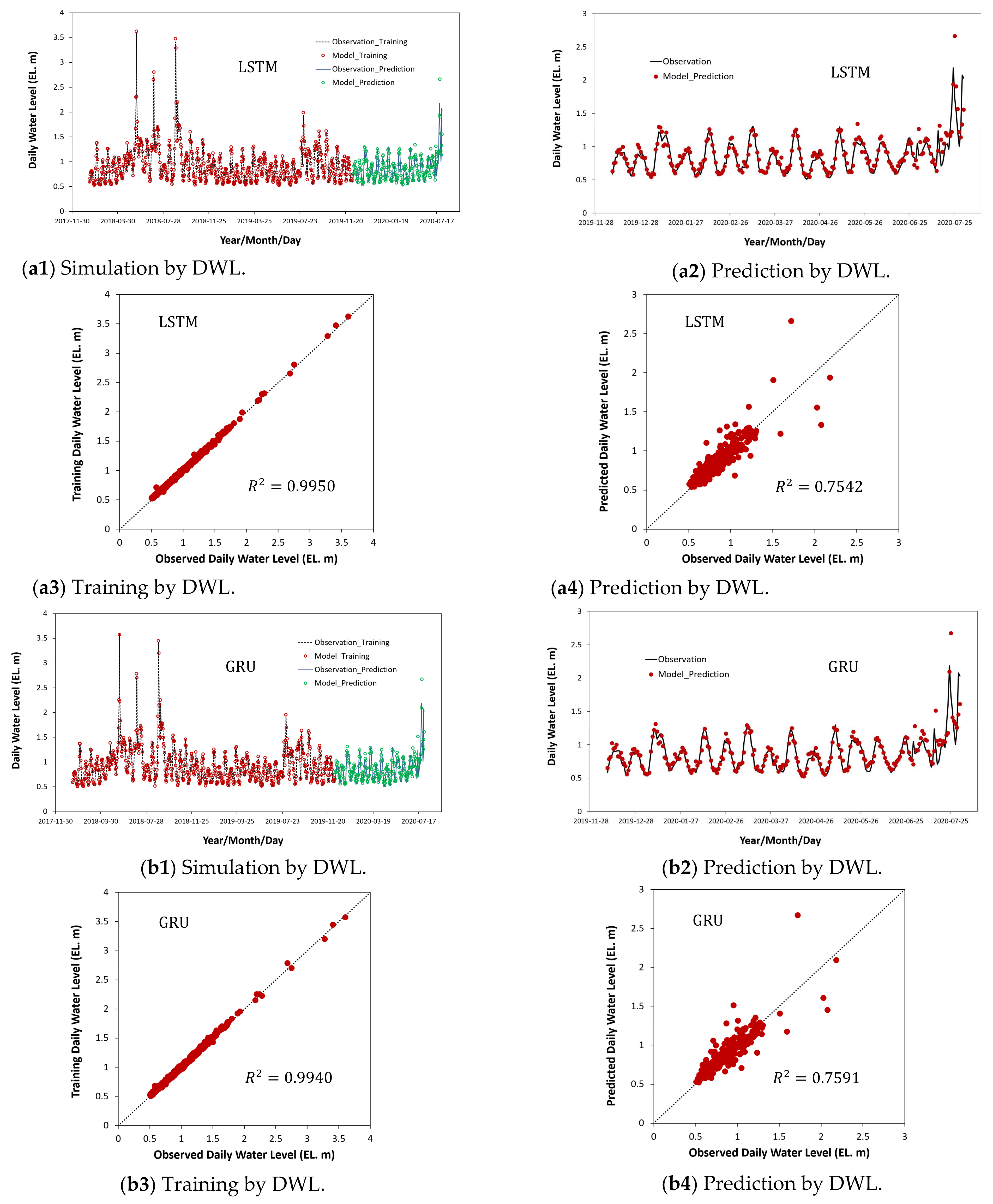
4.1. Results on Training and Prediction Using Water Levels as Univariate Input Data

The learning and prediction results for the two deep learning models (LSTM and GRU) that use univariate time-series learning data are shown in Figure 6 and

Table 8. Comparison of univariate model performance.

Model	Computational State	MAE $(\mathrm{EL}.\mathrm{m})$	MSE $(\mathrm{EL}.\mathrm{m})$	RMSE $(\mathrm{EL}.\mathrm{m})$	${\mathit{R}}^2$	NSE	MRPE $(\mathrm{EL}.\mathrm{m})$
LSTM	Training	0.0136	0.0003	0.0179	0.9950	0.9975	0.0126
	Prediction	0.0824	0.0181	0.1344	0.7542	0.7345	0.0919
GRU	Training	0.0158	0.0004	0.0207	0.9940	0.9966	0.0158
	Prediction	0.0796	0.0171	0.1306	0.7591	0.7362	0.0719

. The red circles in Figure 6(a1,b1) represent the learning results of the models, and the green circles in Figure 6(a1,b1) and the red circles in Figure 6(a2,b2) represent the prediction results of the models. The training and prediction accuracy evaluations of the two models are shown in $R^2$ and are displayed in Figure 6(a3,a4,b3,b4).

The training results of the LSTM and GRU models were very well learned, with an $R^2$ of 0.9950 and 0.9940, respectively. As for the prediction results of the two models (LSTM and GRU), $R^2$ was 0.7542 and 0.7591, respectively. The prediction results of the GRU were evaluated slightly higher in accuracy than those of the LSTM. However, as shown in Figure 6(a2,b2) and Figure 6(a4,b4), the prediction results at high water levels were calculated to be much larger than the observed values for both models. As shown in Table 8, the $NSE$ of the LSTM prediction result is 0.7345, and that of the GRU prediction result is 0.7362. The range of $NSE$s for the predictions presented in Table 1 was not “very good” but “good”, and the accuracy was predicted to be lower than that of the model’s training results. The MRPE presented in Equation (17) was used as an index representing the accuracy of peak values. The learning accuracy at peak water levels was 0.0126 for MRPE in LSTM and 0.0158 for that of GRU. In addition, the peak-water-level prediction accuracy was 0.0719 for MRPE of GRU, which was higher than 0.0919 for that of LSTM.

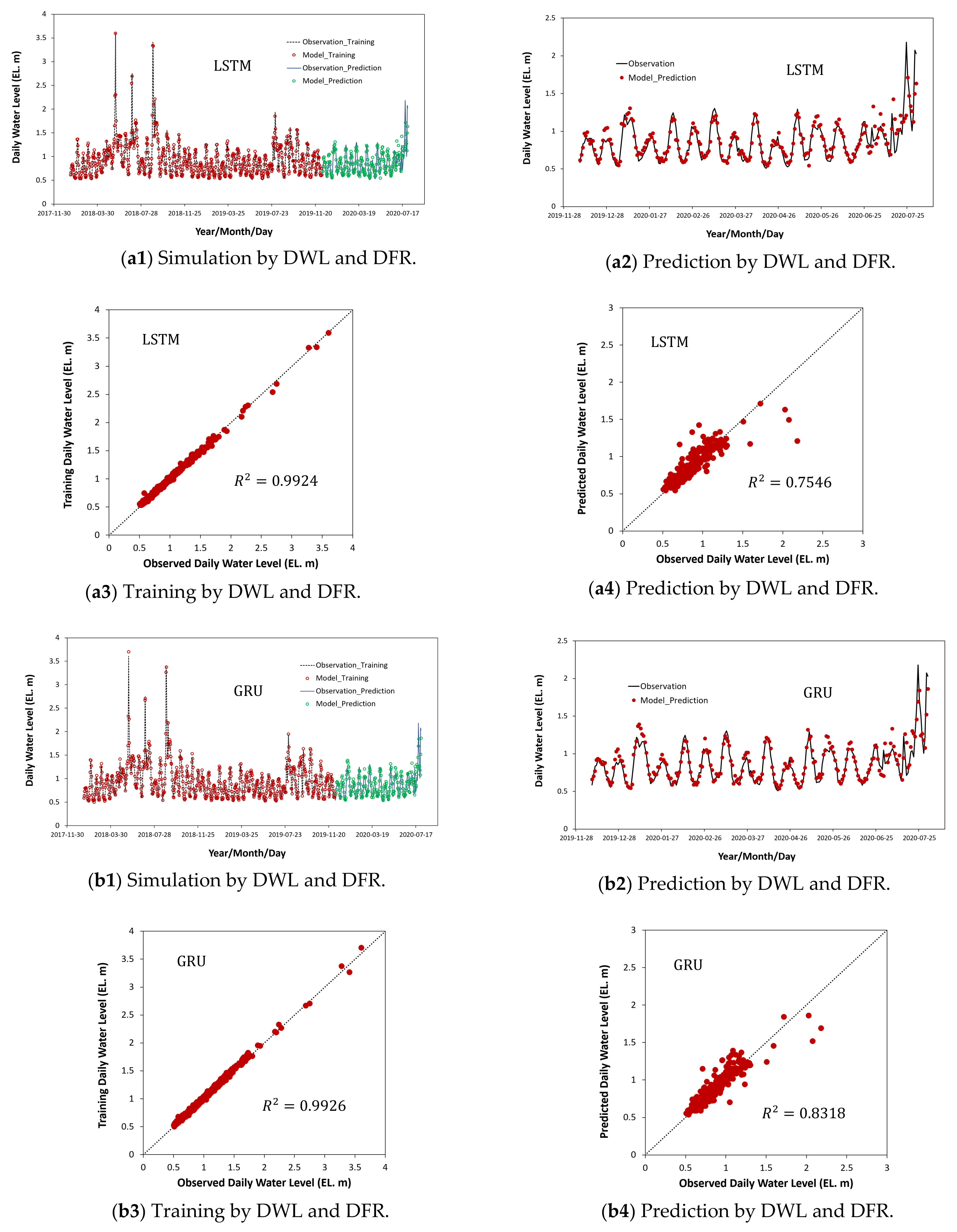
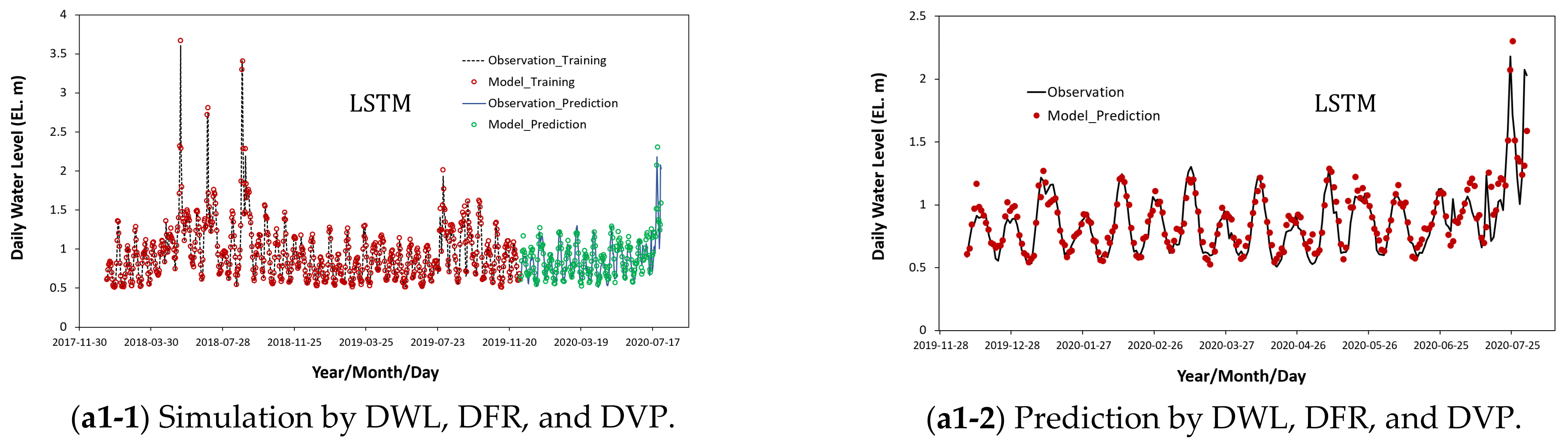
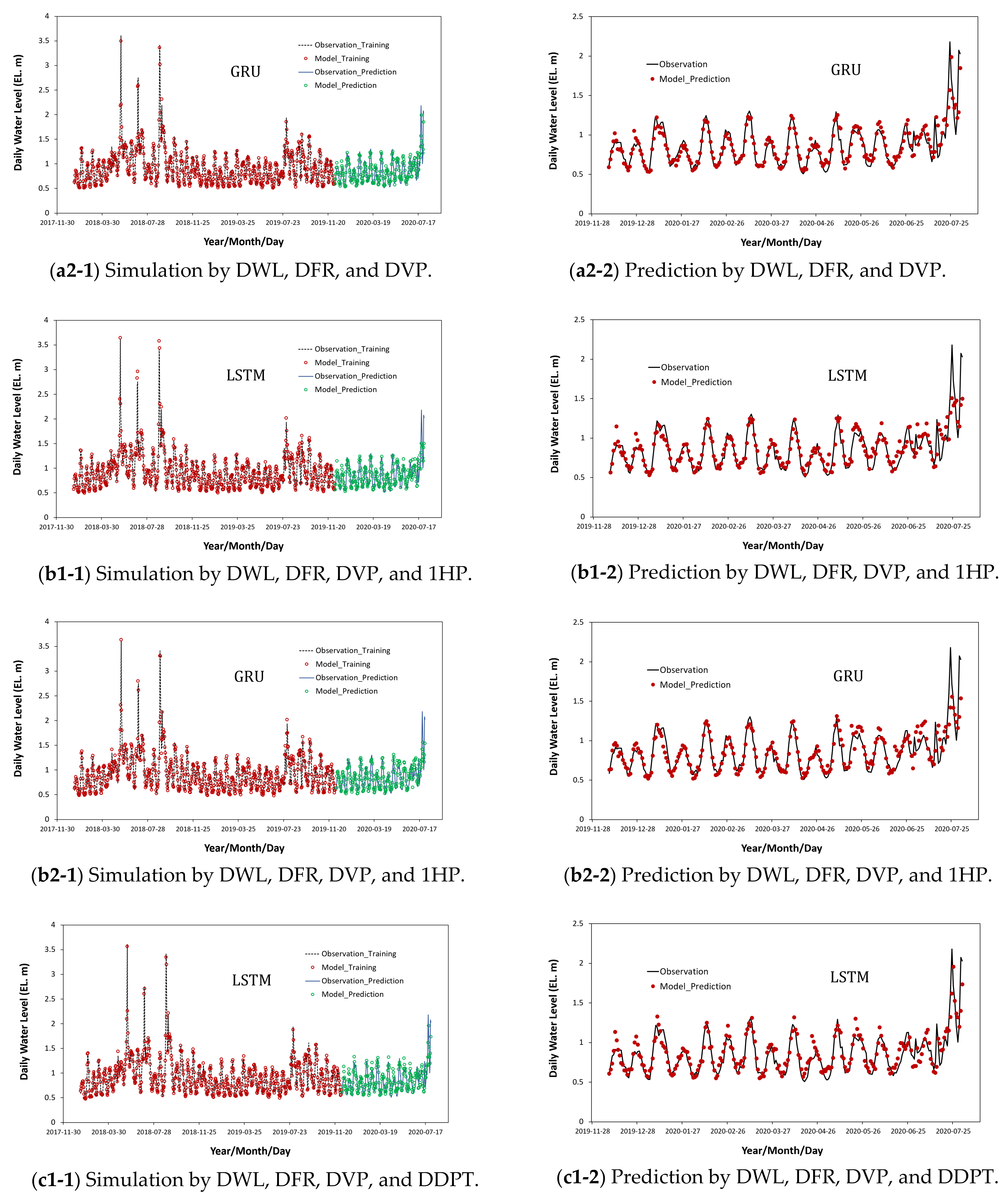
4.2. Results on Training and Prediction Using Water Levels and Flow Rates as Bivariate Input Data

As shown in Figure 7 and

Table 9. Comparison of bivariate model performance.

Model	Computational State	MAE $(\mathrm{EL}.\mathrm{m})$	MSE $(\mathrm{EL}.\mathrm{m})$	RMSE $(\mathrm{EL}.\mathrm{m})$	${\mathit{R}}^2$	NSE	MRPE $(\mathrm{EL}.\mathrm{m})$
LSTM	Training	0.0181	0.0006	0.0245	0.9924	0.9951	0.0177
	Prediction	0.0787	0.0163	0.1278	0.7546	0.6694	0.0887
GRU	Training	0.0200	0.0007	0.0268	0.9926	0.9945	0.0221
	Prediction	0.0719	0.0117	0.1081	0.8318	0.7965	0.0895

, these are the training and prediction results of the two models that use DWL and DFR as bivariate training variables. In both models (LSTM and GRU), the $R^2$s of the training results (Figure 7(a3,b3)) were 0.9924 and 0.9926, which corresponded to “very good” (Table 1). As a result of prediction of the LSTM and GRU models (Figure 7(a4,b4)), $R^2$s were 0.7546 and 0.8318, respectively, and it was confirmed that the accuracy was significantly improved in the bivariate training results considering DFR, for which the data have a greater correlation with DWL than the univariate prediction results. As shown in Figure 7(a2,b2), the predictions of the low water levels in both models were relatively very consistent with the observed values. In addition, in high-water-level predictions, as shown in Figure 7(a2,b2),(a4,b4), the training results of bivariate GRU model including DFR, which correlated with DWL, significantly improved the performance of the prediction. As shown in Table 9, the improvement effect of the bivariate learning result was significantly improved in the prediction result of GRU ($R^2=0.8318;NSE=0.7965$) compared to that of LSTM ($R^2=0.7546;NSE=0.6694$). As shown in Table 9, MRPE for peak-water-level training and prediction of the bivariate model showed values similar to those of the univariate models in Table 8.

4.3. Results on Training and Prediction Using Water Levels and Flow Rates as Multivariate Input Data

Figure 8 and

Table 10. Comparison of multivariate model performance.

Model	Variables	Computational State	MAE $(\mathrm{EL}.\mathrm{m})$	MSE $(\mathrm{EL}.\mathrm{m})$	RMSE $(\mathrm{EL}.\mathrm{m})$	${\mathit{R}}^2$	NSE	MRPE $(\mathrm{EL}.\mathrm{m})$
LSTM	DWL, DFR	Training	0.0181	0.0006	0.0245	0.9924	0.9951	0.0177
		Prediction	0.0787	0.0163	0.1278	0.7546	0.6694	0.0887
GRU	DWL, DFR	Training	0.0200	0.0007	0.0268	0.9926	0.9945	0.0221
		Prediction	0.0719	0.0117	0.1081	0.8318	0.7965	0.0895
LSTM	DWL, DFR, DVP	Training	0.0254	0.0012	0.0342	0.9917	0.9914	0.0239
		Prediction	0.0812	0.0153	0.1235	0.7846	0.7447	0.0966
GRU	DWL, DFR, DVP	Training	0.0261	0.0012	0.0351	0.9887	0.9898	0.0287
		Prediction	0.0710	0.0129	0.1137	0.8033	0.7558	0.1019
LSTM	DWL, DFR, DVP, 1HP	Training	0.0233	0.0011	0.0332	0.9902	0.9919	0.0256
		Prediction	0.0802	0.0157	0.1254	0.7625	0.6547	0.0953
GRU	DWL, DFR, DVP, 1HP	Training	0.0294	0.0016	0.0396	0.9853	0.9883	0.0324
		Prediction	0.0815	0.0166	0.1287	0.7480	0.6688	0.0999
LSTM	DWL, DFR, DVP, DDPT	Training	0.0267	0.0008	0.0283	0.9895	0.9936	0.0228
		Prediction	0.0766	0.0154	0.1240	0.7686	0.7131	0.1104
GRU	DWL, DFR, DVP, DDPT	Training	0.0267	0.0013	0.0359	0.9875	0.9892	0.0232
		Prediction	0.0766	0.0123	0.1110	0.8135	0.7580	0.0882
LSTM	DWL, DFR, DVP, DDPT, 1HP	Training	0.0234	0.0009	0.0303	0.9897	0.9928	0.0217
		Prediction	0.0882	0.0169	0.1301	0.7437	0.6489	0.1271
GRU	DWL, DFR, DVP, DDPT, 1HP	Training	0.0331	0.0019	0.0435	0.9846	0.9857	0.0305
		Prediction	0.0826	0.0129	0.1135	0.8120	0.7524	0.0807

showed the training and prediction results of LSTM and GRU with two or more input variables that are highly correlated with DWL. As shown in Table 10, the $R^2$s of the two or more multivariate training results of the two models correspond to “very good” in the range of 0.9857–0.9951. In both models (LSTM and GRU), except for the case of training of five variables (Figure 8(d1-2),(d2-2)), in two or more multivariate training models, the prediction results of the low water levels were relatively consistent with the observed data (Figure 8(a1-2)–(c2-2)).

As shown in Figure 8(a1-1)–(a2-2), when trivariate training including DFR and DVP, which are data that are directly correlated with DWL, was performed, the prediction accuracy was high not only in the results of GRU ($NSE=0.7558$) but also in those of LSTM ($NSE=0.7447$). In addition, similar to the bivariate training result, the trivariate training result was well matched with the observed data in the high-water-level-prediction result.

As shown in Table 7, the results of the four-variant training were compared with the prediction results including 1HP data that are not directly correlated with DWL in the training data Figure 8(b1-1)–(b2-2) and the prediction results including DDPT data that are directly correlated with DWL (Figure 8(c1-1)–(c2-2)). First, the prediction results in the case of including 1HP data were relatively well matched with the observed values at the low water level, but were underestimated at the high-water-level prediction (Figure 8(b1-2)–(b2-2)). In both LSTM and GRU prediction results, $NSE$s were 0.6547 and 0.6688, respectively, and the prediction performance was significantly reduced. Therefore, it was determined that the 1HP data were difficult to use as appropriate input data for predicting DWL. Second, when the DDPT data were included in the four-variable training data, the prediction accuracy of DWL in both models was greatly improved to $NSE=0.7580$. In high-water-level prediction, selecting DDPT data with a large correlation with DWL could improve the accuracy of high-water-level prediction more than selecting 1HP data with a large correlation with DFR (Figure 8(c1-2),(c2-2)).

Finally, as shown in Table 10, when all five input data are used for learning, the accuracy of predicting high water levels of LSTM was rapidly lowered to $NSE=0.6489$. However, that of GRU was significantly improved to $NSE=0.7524$. However, as shown in Figure 8(d1-2),(d2-2), both models tended to be overestimated compared to the observed values in the low-water-level prediction.

As mentioned in previous research results [4], a more effective model in predicting hydrological time series was GRU. In the results of this study, as shown in Table 10, the prediction result of GRU was higher in prediction accuracy than that of LSTM. The prediction results using two or more multivariate input data of GRU corresponded to “very good”, with NSE ranging from 0.7524 to 0.7965. As shown in Table 10, MRPEs, indexes of peak-water-level-prediction accuracy, were calculated to be more accurate in the range of 0.0807–0.0895 in most cases of GRU than in the case of LSTM.

5. Discussion

The composition of the DNN models input to the model used the calculation conditions of the same model based on the previous results of studying the flow-rate-prediction method with large temporal fluctuations [4]. Based on the results of previous studies, SL, the training unit of data optimally applied to the prediction of hydrological time-series data, used 14 days. In addition, the distribution ratio of learning and prediction data was 74.9% to 25.1%, which was composed and used. Therefore, the water levels were predicted by using 74.9% of the total size of the data as training data.

As seen in previous studies [6,8], despite the training of multivariate data in the cases of multivariate models, it was determined that the rapidly changing water-level-prediction accuracy decreased when predicting the hydrological data without correlation analysis of input data. In this study, DP, which was expected to show a very close correlation with the water level, was analyzed to have a very low correlation coefficient of 0.2993. The reason for this was that the distance between the Seoul Observatory and the Hangang Bridge Station was considerably great, and it was determined that the hydrological and meteorological characteristics were somewhat different. Therefore, in order to generate multivariate training data, it is necessary to first check the homogeneity with the data by analyzing the correlation with the water-level data, which are a prediction target variable.

Other previous data-driven models [5,6,7,8,9,10,20,21,22,23,24,25,26,27,28] significantly degraded predictive performance for rapidly changing high-water-level fluctuations, whereas, in this study, high-water-level predictive-performance evaluations of LSTM and GRU were conducted based on previous study results [4]. The prediction results of the water level using univariate training data in LSTM were more accurate than those using bivariate or trivariate training. The LSTM prediction result did not significantly affect the accuracy improvement of the training result using multivariate input. The prediction results using the trivariants and pentavariants of LSTM deteriorated $NSE$ from 0.6489 to 0.6694. However, in the GRU model, the accuracy was significantly improved in high-water-level predictions as compared to those using univariate ($NSE=0.7362$) in all multivariate predictions ($NSE=0.7524–0.7965$), except for one case that used tetravariants (i.e., DWL, DFR, DVP, and 1HP) ($NSE=0.6688$). In contrast to previous studies [4,5,6,7,8,9,10,11,12,13,14,15,16,17,18,19,20,21,22,23,24,25,26,27,28,29,30], MRPE, a quantitative indicator for evaluating peak-water-level accuracy, was used to grasp the rapidly changing water-level-prediction accuracy. In the case of the GRU, not only the univariate model but also the multivariate models with large correlation had high accuracy of peak-water-level prediction ($MRPE=0.0807–0.0895$).

The prediction results of the LSTM and GRU were as follows by selecting training data that were close to the correlation of water-level data. The prediction results of the LSTM were very effective in predicting by using univariate input data, and the accuracy was high, but high-water-level predictions tended to be overestimated compared to observations. The prediction results of the GRU were predicted with high accuracy in both the univariate and multivariate inputs, but the overestimation of the high water level in the prediction using only the univariate input data was the same as that of the LSTM. Therefore, even with the GRU model, in order to increase the accuracy of the high-water-level predictions, other hydrological and meteorological data that are highly correlated with the water levels were supplemented with input data to improve the accuracy of time-series water-level prediction over the entire range.

6. Conclusions

This study looked at the development of flood-prediction technology in response to the rapid increase in direct runoff to urban rivers that results from both climate change and urban development projects around rivers. In particular, in the case of rivers with severe temporal fluctuations, accurate water-level prediction should be possible. Therefore, using data-driven models (i.e., LSTM and GRU), it was possible to propose an effective and accurate data model for predicting water levels with severe temporal changes.

In this study, DWL, DFR, DVP, DDPT, and 1HP were selected as hydrological and meteorological input data to the model in the order of data that correlated with the water level to be predicted. The input dataset of LSTM and GRU was generated by combining the selected hydrological and meteorological data. The accuracy of water-level prediction was evaluated by applying LSTM and GRU, which are suitable deep-learning techniques for predicting time-series hydrological data for accurate high-water-level prediction. In the case of LSTM, the accuracy of high-water-level prediction by univariate water-level input was higher than that of the multivariate model. On the other hand, GRU was able to select a model suitable for predicting multivariate time-series water levels because the high-water-level-prediction accuracy of multivariate models was evaluated higher than prediction accuracy under univariate input conditions.

The results of this study showed that the accuracy of the predicted water level could be improved in the GRU when multivariate hydrological and meteorological data were secured in urban rivers with high-water-level fluctuations. Therefore, the multivariate learning result, which has a greater correlation with the water level than the univariate learning result using only the water level, could accurately predict the water level as “very good” ($NSE=0.7524–0.7965;MRPE=0.0807–0.0895$).

In this study, the selected RNNs (i.e., LSTM and GRU) were data-driven models that analyzed the numerical variability of data rather than the physical characteristics of data. In addition, learning only univariate data greatly reduces the prediction accuracy of time-series data with rapidly temporal fluctuations, so if there is a multivariate model that uses variables with high correlation with predictive data as input data, it can be expanded to rapidly changing hydrological-data-prediction studies.

References

1. Lee, K.S. Rehabilitation of the Hydrologic Cycle in the Anyangcheon Watershed; Sustainable Water Resources Research Center, Ministry of Education, Science and Technology: Seoul, Korea, 2007. [Google Scholar]
2. Lee, K.S.; Chung, E.S. Development of integrated watershed management schemes for an intensively urbanized region in Korea. J. Hydro Environ. Res. 2007, 1, 95–109. [Google Scholar] [CrossRef]
3. Henonin, J.; Russo, B.; Mark, O.; Gourbesville, P. Real-time urban flood forecasting and modelling—A state of the art. J. Hydroinform. 2013, 15, 717–736. [Google Scholar] [CrossRef]
4. Park, K.; Jung, Y.; Kim, K.; Park, S.K. Determination of deep learning model and optimum length of training data in the river with large fluctuations in flow rates. Water 2020, 12, 3537. [Google Scholar] [CrossRef]
5. Irvine, K.N.; Eberhardt, A.J. Multiplicative, seasonal ARIMA models for Lake Erieand Lake Ontario water levels. JAWRA J. Am. Water Resour. Assoc. 1992, 28, 385–396. [Google Scholar] [CrossRef]
6. Tokar, A.S.; Johnson, P.A. Rainfall-runoff modeling using artificial neural networks. J. Hydrol. Eng. ASCE 1999, 4, 232–239. [Google Scholar] [CrossRef]
7. Yan, Q.; Ma, C. Application of integrated ARIMA and RBF network for groundwater level forecasting. Environ. Earth Sci. 2016, 75, 396. [Google Scholar] [CrossRef]
8. Shirmohammadi, B.; Vafakhah, M.; Moosavi, V.; Moghaddamnia, A. Application of several data-driven techniques for predicting groundwater level. Water Resour. Manag. 2013, 27, 419–432. [Google Scholar] [CrossRef]
9. Hasebe, M.; Nagayama, Y. Reservoir operation using the neural network and fuzzy systems for dam control and operation support. Adv. Eng. Softw. 2002, 33, 245–260. [Google Scholar] [CrossRef]
10. Chang, F.J.; Chang, Y.T. Adaptive neuro-fuzzy inference system for prediction of water level in reservoir. Adv. Water Resour. 2006, 29, 1–10. [Google Scholar] [CrossRef]
11. Tran, Q.-K.; Song, S.-K. Water level forecasting based on deep learning: A use case of Trinity River-Texas-the United States. J. KIISE 2017, 44, 607–612. [Google Scholar] [CrossRef]
12. Kumar, D.N.; Raju, K.S.; Sathish, T. River flow forecasting using recurrent neural networks. Water Resour. Manag. 2004, 18, 143–161. [Google Scholar] [CrossRef]
13. Firat, M. Comparison of artificial intelligence techniques for river flow forecasting. Hydrol. Earth Syst. Sci. 2008, 12, 123–139. [Google Scholar] [CrossRef] [Green Version]
14. Sattari, M.T.; Yurekli, K.; Pal, M. Performance evaluation of artificial neural network approaches in forecasting reservoir inflow. Appl. Math. Model. 2012, 36, 2649–2657. [Google Scholar] [CrossRef]
15. Chen, P.-A.; Chang, L.-C.; Chang, L.-C. Reinforced recurrent neural networks for multi-step-ahead flood forecasts. J. Hydrol. 2013, 497, 71–79. [Google Scholar] [CrossRef]
16. Zhang, D.; Peng, Q.; Lin, J.; Wang, D.; Liu, X.; Zhuang, J. Simulating reservoir operation using a recurrent neural network algorithm. Water 2019, 11, 865. [Google Scholar] [CrossRef] [Green Version]
17. Mok, J.-Y.; Choi, J.-H.; Moon, Y.-I. Prediction of multipurpose dam inflow using deep learning. J. Korea Water Resour. Assoc. 2020, 53, 97–105. [Google Scholar]
18. Zhang, D.; Lin, J.; Peng, Q.; Wang, D.; Yang, T.; Sorooshian, S.; Liu, X.; Zhuang, J. Modeling and simulating of reservoir operation using the artificial neural network, support vector regression, deep learning algorithm. J. Hydrol. 2018, 565, 720–736. [Google Scholar] [CrossRef] [Green Version]
19. Apaydin, H.; Feizi, H.; Sattari, M.T.; Colak, M.S.; Shamshirband, S.; Chau, K.-W. Comparative analysis of recurrent neural network architectures for reservoir inflow forecasting. Water 2020, 12, 1500. [Google Scholar] [CrossRef]
20. Adamowski, J.; Chan, H.F. A wavelet neural network conjunction model for groundwater level forecasting. J. Hydrol. 2011, 407, 28–40. [Google Scholar] [CrossRef]
21. Partal, T.; Cigizoglu, H.K. Estimation and forecasting of daily suspended sediment data using wavelet-neural networks. J. Hydrol. 2008, 358, 317–331. [Google Scholar] [CrossRef]
22. Rajaee, T.; Nourani, V.; Mohammad, Z.K.; Kisi, O. River suspended sediment load prediction: Application of ANN and wavelet conjunction model. J. Hydrol. Eng. 2011, 16, 613–627. [Google Scholar] [CrossRef]
23. Adnan, R.; Ruslan, F.A.; Samad, A.M.; Zain, Z.M. Flood Water Level Modelling and Prediction Using Artificial Neural Network: Case Study of Sungai Batu Pahat in Johor. In Proceedings of the 2012 IEEE Control and System Graduate Research Colloquium, Shah Alam, Malaysia, 16–17 July 2012; pp. 22–25. [Google Scholar]
24. Rezaeianzadeh, M.; Kalin, L.; Hantush, M. An integrated approach for modeling wetland water level: Application to a headwater wetland in coastal Alabama, USA. Water 2018, 10, 879. [Google Scholar] [CrossRef] [Green Version]
25. Choi, C.; Kim, J.; Han, H.; Han, D.; Kim, H.S. Development of water level prediction models using machine learning in wetlands: A case study of Upo wetland in South Korea. Water 2020, 12, 93. [Google Scholar] [CrossRef] [Green Version]
26. Kisi, O.; Shiri, J.; Nikoofar, B. Forecasting daily lake levels using artificial intelligence approaches. Comput. Geosci. 2012, 41, 169–180. [Google Scholar] [CrossRef]
27. Hipni, A.; El-Shafie, A.; Najah, A.; Karim, O.A.; Hussain, A.; Mukhlisin, M. Daily forecasting of dam water levels: Comparing a support vector machine (SVM) model with adaptive neuro fuzzy inference system (ANFIS). Water Resour. Manag. 2013, 27, 3803–3823. [Google Scholar] [CrossRef]
28. Young, C.C.; Liu, W.C.; Hsieh, W.L. Predicting the water level fluctuation in an Alpine Lake using physically based, artificial neural network, and time series forecasting models. Math. Probl. Eng. 2015, 2015, 708204. [Google Scholar] [CrossRef] [Green Version]
29. Guo, F.; Yang, J.; Li, H.; Li, G.; Zhang, Z. A ConvLSTM conjunction model for groundwater level forecasting in a karst aquifer considering connectivity Characteristics. Water. 2021, 13, 2759. [Google Scholar] [CrossRef]
30. Di Nunno, F.; Granata, F.; Gargano, R.; de Marinis, G. Forecasting of extreme storm tide events using NARX neural network-based models. Atmosphere 2021, 12, 512. [Google Scholar] [CrossRef]
31. Di Nunno, F.; de Marinis, G.; Gargano, R.; Granata, F. Tide prediction in the Venice Lagoon using Nonlinear Autoregressive Exogenous (NARX) neural network. Water 2021, 13, 1173. [Google Scholar] [CrossRef]
32. Liu, Y.; Wang, H.; Feng, W.; Huang, H. Short term real-time rolling forecast of urban river water levels based on LSTM: A case study in Fuzhou City, China. Int. J. Environ. Res. Public Health 2021, 18, 9287. [Google Scholar] [CrossRef]
33. Hochreiter, S.; Schmidhuber, J. Long Short-Term Memory. Neural Comput. 1997, 9, 1735–1780. [Google Scholar] [CrossRef] [PubMed]
34. Cho, K.; Van Merrienboer, B.; Bahdanau, D.; Bengio, Y. On the Properties of Neural Machine Translation: Encoder–Decoder Approaches. In Proceedings of the SSST-8, Eighth Workshop on Syntax, Semantics and Structure in Statistical Translation, Doha, Qatar, 7 October 2014; pp. 103–111. [Google Scholar]
35. Moriasi, D.N.; Arnold, J.G.; Van Liew, M.W.; Bingner, R.L.; Harmel, R.D.; Veith, T.L. Model evaluation guidelines for systematic quantification of accuracy in watershed simulations. Soil Water Div. ASABE 2007, 50, 885–900. [Google Scholar]
36. Segura-Beltrán, F.; Sanchis-Ibor, C.; Morales-Hernández, M.; González-Sanchis, M.; Bussi, G.; Ortiz, E. Using post-flood surveys and geomorphologic mapping to evaluate hydrological and hydraulic models: The flash flood of the Girona River (Spain) in 2007. J. Hydrol. 2016, 541, 310–329. [Google Scholar] [CrossRef] [Green Version]
37. Kastridis, A.; Kirkenidis, C.; Sapountzis, M. An integrated approach of flash flood analysis in ungauged Mediterranean watersheds using post-flood surveys and unmanned aerial vehicles. Hydrol. Process. 2020, 34, 4920–4939. [Google Scholar] [CrossRef]
38. Narbondo, S.; Gorgoglione, A.; Crisci, M.; Chreties, C. Enhancing physical similarity approach to predict runoff in ungauged watersheds in sub-tropical regions. Water 2020, 12, 528. [Google Scholar] [CrossRef] [Green Version]
39. Chen, H.; Luo, Y.; Potter, C.; Moran, P.J.; Grieneisen, M.L.; Zhang, M. Modeling pesticide diuron loading from the San Joaquin watershed into the Sacramento-San Joaquin Delta using SWAT. Water Res. 2017, 121, 374–385. [Google Scholar] [CrossRef]
40. Chiew, F.; Stewardson, M.J.; McMahon, T. Comparison of six rainfall-runoff modelling approaches. J. Hydrol. 1993, 147, 1–36. [Google Scholar] [CrossRef]
41. Al-Smadi, M. Incorporating Spatial and Temporal Variation of Watershed Response in a GIS-based Hydrological Model. Master’s Thesis, Virginia Institute of Technology, Blacksburg, VA, USA, 1998. [Google Scholar]
42. Seoul Metropolitan Government. Study on River Management by Universities; Seoul Metropolitan Government: Seoul, Korea, 2013.
43. Seoul Metropolitan Government. Statistical Yearbook of Seoul; Seoul Metropolitan Government: Seoul, Korea, 2004.
44. Ministry of Construction and Transportation. Master Plan for River Modification of the Han River Basin; Ministry of Construction and Transportation: Seoul, Korea, 2002.
45. Water Resources Management Information System. Hydrological Data. Available online: http://www.wamis.go.kr (accessed on 1 August 2021).
46. Korea Meteorological Administration, National Climate Data Center. Meteorological Data. Available online: https://data.kma.go.kr (accessed on 1 August 2021).
47. Google Earth. Available online: http://www.google.com/maps (accessed on 1 October 2021).
48. Lee, J.S. Water Resources Engineering; Goomibook: Seoul, Korea, 2008. [Google Scholar]
49. Anaconda. Python. Available online: https://www.anaconda.com (accessed on 1 August 2021).
50. TensorFlow. TensorFlow. Available online: https://www.tensorflow.org (accessed on 1 August 2021).
Figure 1. Long Short-Term Memory (LSTM).
Water 14 00469 g001
Figure 2. Gated Recurrent Unit (GRU).
Water 14 00469 g002
Figure 3. Flowchart on learning and prediction of water-level data, using LSTM and GRU models.
Water 14 00469 g003
Figure 4. Map of the Han River basin in Korea (Google Earth [47]).
Water 14 00469 g004
Figure 5. Time-series daily water level at the Hangang Bridge (period: 2018–2020).
Water 14 00469 g005
Figure 6. Observed and computed total time series water levels (a1) and (b1) as univariate input data, prediction (a2) and (b2) as univariate input data, R 2   for training (a3) and (b3), and R 2   for prediction (a4) and (b4): (a1a4) Long Short-Term Memory (LSTM); and (b1b4) Gated Recurrent Unit (GRU).
Water 14 00469 g006
Figure 7. Observed and computed total time series water levels (a1) and (b1) as bivariate input data, prediction (a2) and (b2) as bivariate input data, R 2   for training (a3) and (b3), and R 2   for prediction (a3) and (b3): (a1a4) LSTM; and (b1b4) GRU.
Water 14 00469 g007
Figure 8. Observed and training total time-series water levels as multivariate input data: (a1-)–(d1-) LSTM; and (a2-)–(d2-) GRU.
Water 14 00469 g008aWater 14 00469 g008bWater 14 00469 g008c