Article

Remote Analysis of the Chlorophyll-a Concentration Using Sentinel-2 MSI Images in a Semiarid Environment in Northeastern Brazil

by
Thaís R. Benevides T. Aranha
1,*,
Jean-Michel Martinez
2,
Enio P. Souza
3,
Mário U. G. Barros
4 and
Eduardo Sávio P. R. Martins
5
1
Department of Hydraulic and Environmental Engineering, Federal University of Ceará, Campus do Pici, Block 713, Fortaleza 60440-970, Ceará, Brazil
2
Géosciences Environnement Toulouse (GET), Unité Mixte de Recherche 5563, IRD/CNRS/Université, 31400 Toulouse, France
3
Department of Atmospheric Sciences, Federal University of Campina Grande, Campina Grande 58429-140, Paraíba, Brazil
4
Water Resources Management Company (COGERH), Fortaleza 60824-140, Ceará, Brazil
5
Research Institute of Meteorology and Water Resources (FUNCEME), Fortaleza 60115-221, Ceará, Brazil
*
Author to whom correspondence should be addressed.
Water 2022, 14(3), 451; https://doi.org/10.3390/w14030451
Submission received: 8 December 2021 / Revised: 21 January 2022 / Accepted: 29 January 2022 / Published: 2 February 2022

Abstract

:
In this paper, the authors use remote-sensing images to monitor the water quality of reservoirs located in the semiarid region of Northeast Brazil. Sentinel-2 MSI TOA Level 1C reflectance images were used to remotely estimate the concentration of chlorophyll-a (chl-a), the main indicator of the trophic state of aquatic environments, in five reservoirs in the state of Ceará, Brazil. A three-spectral band retrieval model was calibrated using 171 water samples, collected from November 2015 through July 2018 in 5 reservoirs. For validation, 71 additional samples, collected from August 2018 through December 2019, were used to ensure a robust accuracy assessment. The TOA Level 1C products performed very well, achieving a relative RMSE of 28% and R2 = 0.80. Data on wind direction and speed, solar radiation and reservoir volume were used to generate a conceptual model to analyze the behavior of chl-a in the surface waters of the Castanhão reservoir. During 2019, the reservoir water quality showed strong variation, with concentration fluctuating from 30 to 95 µg/L We showed that the end of the dry season is marked by strong eutrophic conditions corresponding to very low water inflows into the reservoir. During the rainy season there is a large decrease in the chl-a concentration following the increase of the lake water storage. During the following dry season, satellite data show a progressive improvement of the trophic state controlled by wind intensity that promotes a better mixing of the reservoir waters and inhibiting the development of most phytoplankton.

1. Introduction

The Brazilian semiarid portion covers an area of about 1 million km2, which corresponds to 86% of the Northeast region of Brazil [1]. This region has irregular rainfall and high temperatures, with more than 2800 h of sunshine per year, in addition to high evaporation rates, around 2000 mm per year [2]. The soil is predominantly crystalline, and this is one of the factors responsible for the low levels of groundwater availability as well as the low quality of water accumulated in the aquifers, due to the high levels of salts from this type of rock [3].
Due to the strong interannual rainfall variability and the overall scarcity of rainfall in addition to unfavorable soil conditions, the construction of reservoirs such as weirs and dams to store water during the rainy season, and of water transposition channels to take this resource to the locations most affected by the drought, appeared as a reliable alternative to mitigate water scarcity in this semiarid region. Hence, construction of reservoirs is central to the storage and distribution of water in arid and semiarid regions. However, this intervention in the natural landscape, resulting from the transformation of lotic to lentic environments, entails a series of impacts on ecosystems, with changes in the natural behavior and water quality of engineered rivers and streams [4]. This anthropogenic interference generates a great ecological impact on aquatic ecosystems by reducing the flow of water, and increasing the sedimentation rate, water residence time, thermal stratification, and artificial enrichment of nutrients such as nitrogen and phosphorus (eutrophication) caused by human activities [5,6].
Eutrophication presents changes in the physicochemical and biological characteristics of these aquatic environments, arising from the use of fertilizers and pesticides in agriculture, the discharge of industrial and domestic sewage without adequate treatment, destruction of riparian vegetation in water sources, and high urbanization rate. This process produces changes in water quality, such as reduced dissolved oxygen, fish death, excessive proliferation of phytoplanktonic organisms and, consequently, increased incidence of potentially toxin-producing algae and cyanobacterial blooms [7,8]. Given this scenario, the concern with the degradation of these aquatic environments has grown in the scientific community, making it necessary to increase studies and expand knowledge on the subject.
Phytoplankton refers to the set of microscopic aquatic organisms that have photosynthetic capacity and that live dispersed floating in the water column. This group includes organisms traditionally considered algae. However, among these, there is a group of great public health importance, which is also classified as bacteria, namely the cyanobacteria [9,10]. The occurrence of cyanobacterial blooms in water bodies used for urban supply can represent a serious risk to the health of the population, due to the ability of these organisms to produce toxins (cyanotoxins), which can be lethal to mammals and other warm-blooded animals [11,12,13]. Blooms can also interfere with the balance of aquatic ecosystems, as when algae are in suspension they can modify the water’s transparency, which can lead to deoxygenation of the water body and, consequently, fish mortality. In addition, they represent a serious problem for water treatment plants, as they can cause loss of filter load and change in the odor and taste of treated water [14].
Chlorophyll is the photosynthetic pigment present in all phytoplankton organisms. Chlorophyll-a (chl-a) is the most common of the chlorophylls (a, b, c, and d) and represents approximately 1 to 2% of the dry weight of the organic material in all algae. For this reason, knowledge of its concentration is used to detect algal blooms and understand its dynamics [15,16], and to estimate primary productivity [17].
Thus, chl-a is the main indicator of the trophic status of aquatic environments [18,19]. This statement is confirmed for the calculation of the Trophic State Index (TSI), which aims to classify water bodies in different degrees of trophy. The oligotrophic state is characterized by the lowest TSI values, with TSI values increasing through the mesotrophic, eutrophic, to the hypereutrophic, with the highest TSI values. In other words, the TSI aims to assess water quality in terms of nutrient enrichment and its effect related to the overgrowth of algae and cyanobacteria [20]. This index was adopted by [20] for temperate climates and was adapted for lentic environments of tropical climate by [21], using only two variables, namely chl-a and total phosphorus. In this index, the results corresponding to phosphorus should be understood as a measure of the eutrophication potential, since this nutrient acts as the causative agent of the process. The evaluation corresponding to chl-a, on the other hand, should be considered a measure of the response of the water body to the causative agent, adequately indicating the level of algae growth. Thus, the average index satisfactorily encompasses the cause and effect of the process.
As a result, there has been increasing interest in studies of this compound and its derivatives. On the one hand, the irregular nature of the distribution of phytoplankton, in particular the proliferation of cyanobacteria, is characterized by frequent migration dynamics in the vertical layers. In addition to very fast replication rates, this dynamic makes it difficult to carry out a quantitative monitoring of the number of cells and spatiotemporal distribution, as surface blooms can appear and disappear quickly, usually within a few hours [22,23,24]. This poses an appreciable challenge to any research effort for larger water bodies. Normally, measurements for analyzing the quality of water in reservoirs are carried out by collecting water from strategic points, usually near the reservoir banks. These samples do not comprise the entire extent of the dams, and thus may not represent the real spatial distribution of water quality. In addition, these collections are carried out over a long-time interval, often without periodicity [25,26,27].
In this context, remote sensing (RS) reinforces the ability to monitor and understand the composition and dynamics of small and large reservoirs, especially with the advancement of this technology in recent decades. The latest generation of mid-resolution multispectral sensors, with free image availability, such as the Landsat-8 (L8) and Sentinel-2 (S2) satellites, offer advanced opportunities for synoptic view of the entire area of interest, fine-scale, and high-frequency monitoring [28]. These satellites were not specifically designed for water observation but are promising for a detailed analysis of water quality [15,29,30], thanks to their fine radiometric sensitivity [31,32]; 10 to 30-m spatial resolution; high revisit frequency (every 2–3 days combining L8 and S2 satellites) and the improved configuration of the spectral bands in the visible and near infrared range [33].
Orbital sensors are able to record the effects of the interaction of solar radiation with constituents in water [34], and the spectral information contained in satellite images is useful in the development of bio-optical models [35]. Optically active constituents (OACs) such as suspended solids, photosynthetic pigments (chlorophyll), and colored dissolved organic matter (CDOM) are used as indicators of water quality during the characterization of the aquatic environment [36]. The RS applied to the study and monitoring of aquatic environments is based on the processes of selective absorption and scattering of solar radiation by water and its OACs [37,38]. Thus, OACs concentrations can be estimated empirically or semi-analytically, based on RS data [39].
Phytoplankton is capable of synthesizing organic matter from photosynthesis, being mainly responsible for the primary production of cells, causing changes in the spectral behavior of water [40,41]. In general, photosynthetic pigments take advantage of radiation from the blue and red region for the photosynthesis process. Thus, waters with phytoplankton have two bands of maximum absorption in the electromagnetic spectrum, one in the blue region, around 440 nm, and the other in the red region, around 670 nm. The green band, around 560 nm, due to its low absorption coefficient, indicates a high chlorophyll reflectance. In addition, the presence of phytoplankton is also characterized by its peak reflectance at 700 nm, in the near infrared region [42,43,44,45,46].
Importantly, there is a consensus that harmful algal blooms are complex events, normally caused by several environmental factors that occur simultaneously [47]. In addition to the environmental conditions generated by anthropogenic activities, hydrological and climatic variables play an important role in the behavior of phytoplankton [48]. These organisms are sensitive to water-level fluctuations, regarding the abundance, composition and diversity of biomass [49,50,51,52,53], as this changes the physicochemical conditions of water such as the mixing regime, light availability, and nutrient concentrations [54,55,56].
Studies have shown that low water levels together with the high retention time in reservoirs in semiarid regions, resulting from irregularity in precipitation, are often associated with high algal biomass in freshwater ecosystems, due to the high availability of nutrients for primary producers [57,58,59,60,61,62,63,64].
These conditions combined with high irradiation and high temperatures, although they do not result in greater overall phytoplankton biomass, considerably favor the growth of cyanobacteria, which are extremely harmful to human health [65,66,67,68]. As temperatures approach and exceed 20 °C, growth rates of freshwater eukaryotic phytoplankton generally stabilize or decline, while growth rates of many cyanobacteria increase [69,70,71,72], providing a competitive advantage due to physiological factors such as faster growth and physical factors such as improved stratification [73,74,75].
On the other hand, the reduction of the water level can also increase the resuspension of sediments due to the turbulence caused by the wind and, consequently, the increase in inorganic turbidity. This reduces the availability of light and phytoplankton biomass, changing the structure of the phytoplankton community [76,77,78,79].
This study aims at the development of a water-quality analysis methodology based on remote sensing. It is applied to a semiarid environment, strongly influenced by an irregular hydrological regime. The objective is to reproduce trophic variations of water reservoirs of a semiarid region by applying a retrieval algorithm that estimates the concentration of chl-a from Sentinel-2 images. For this purpose, an empirical spectral model will be developed, in which statistical relationships are established between chl-a concentration data collected in situ and the reflectance of spectral bands extracted from Sentinel-2 images. An analysis with hydroclimatic data is also carried out in an attempt to better understand and characterize the eutrophication of the Castanhão reservoir. Section 2 presents the available data and the methodology while results are presented and discussed in Section 3; and, finally, conclusions are presented in Section 4.

2. Data and Methodology
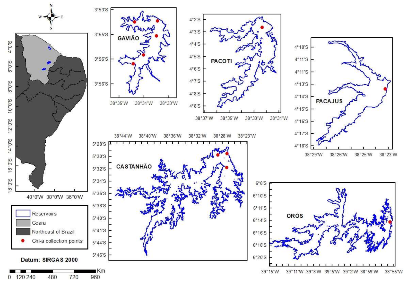
2.1. Study Sites

This study was carried out in the state of Ceará, located in the semiarid region of northeastern Brazil, close to the Equator. The studied reservoirs were Gavião, Pacoti, Pacajús, Castanhão, and Orós. The first three reservoirs are closer to the metropolitan region of Fortaleza (capital of Ceará), and comprise the integrated Gavião system, responsible for the water supply of the metropolitan region. Castanhão and Orós are the two largest reservoirs in Ceará (Castanhão is the largest). Both are located in the Jaguaribe River Basin and play a key role in water security and in flood control of the Jaguaribe valley, in addition to transferring these accumulated waters to the reservoirs in the metropolitan region of Fortaleza. Thus, they are a strategic water reserve for the state. Despite their storage capacity, a severe drought, such as that which occurred between 2012 and 2018, could lead these large reservoirs to have very low volumes of stored water. In 2019 and 2020, Castanhão reached 2.8% and 2.4%, respectively, and Orós 5.2% and 4.7%, respectively, of its water volume capacity [80]. These conditions significantly affect the state’s water supply management and these reservoirs’ water quality.
The climate of this region is hot and dry, and the rainfall is irregular in space and time [81]. It is concentrated between the months of February and May [82], with maximum values in the months March and April [83]. Due to recurrent droughts and high annual average temperature, around 31 °C, it has a negative water balance for most of the year, with high potential evaporation rates, reaching over 2000 mm year−1, and precipitation below 900 mm year−1 [84]. Moreover, the region is characterized by shallow soils on a crystalline basement. All this combined results in intermittent rivers [85,86].
In order to promote greater water security, the construction of surface reservoirs has been the most common and important strategy adopted [87]. These reservoirs, however, are subject to long periods of low, or even, zero inflows and long water residence time (more than 12 months), high solar radiation and high temperatures during most of the rainy season, in addition to intense anthropogenic activity in their basins. These factors contribute to an intense accumulation and concentration of nutrients, making these systems considerably more vulnerable to eutrophication [88]. In order to analyze different water-quality conditions, this study was carried out in reservoirs in which total water-storage capacity varies from 32.9 million to 6.7 billion m³ and trophic state ranges from mesotrophic to hypereutrophic, as shown in Table 1.

2.2. Data

Over decades of satellite water monitoring, remote monitoring of small reservoirs has been greatly hampered by the lack of appropriate satellite sensors [89]. Ocean color sensors such as the MODIS (MODerate Resolution Imaging Spectroradiometer) and the MERIS (Medium Resolution Imaging Spectrometer) have a spatial resolution of 250–1200 m, making them suitable only for very large reservoirs. The first Landsat series satellites (Landsat 1–7) had good spatial resolution (30–79 m) but restricted radiometric resolution (6–8 bits), which made them a limited tool for mapping water-quality parameters [90]. The radiometric resolution of Landsat 8 is 12 bits, and this makes it suitable for remote analysis even in dark lakes (rich in CDOM). However, its revisit time is quite long (16 days), limiting its use in systematic water quality monitoring [91].
In 2015, the launch of the Multispectral Imager (MSI), aboard satellite Sentinel-2, opened up a new potential for the use of RS for reservoir monitoring [92]. The images have a spatial resolution of 10 m, 20 m, and 60 m, which means that even small reservoirs can be studied. Data are acquired in 13 spectral bands, distributed along the visible and infrared regions. This includes narrow bands that capture phytoplankton spectral characteristics, such as the chl-a absorption maximum, around 670 nm, and the reflectance peak near 700 nm associated with phytoplankton backscatter. The radiometric resolution of the sensor is 12 bits. Sentinel-2 comprises a constellation of two identical satellites that are part of the European Commission Copernicus program and operated by the European Space Agency (ESA), located in Paris, France. They operate simultaneously in the same sun-synchronized polar orbit and, in opposite 180° positions, are designed to provide a high 5-day revisit frequency, which makes them suitable for routine monitoring.
In this study, WGS84 UTM zone 24 South images of the Sentinel-2 satellite with a resolution of 10 m were used. The passage date was the closest to the dates of chl-a sample collection in the reservoir, in the period from November 2015 to December 2019. The S2 MSI Level 1C (L1C) images were obtained from the Copernicus Open Access Hub (https://scihub.copernicus.eu/, accessed on 9 September 2021). The Sentinel Application Platform (SNAP) version 7.0 on Windows 10 (64-bit) was used to process the images and the Band Maths function to generate the chl-a concentration maps from the chl-a recovery algorithm.
To calibrate and validate the empirical models, data from in situ chl-a collection were used, provided by the Ceará Water Resources Management Company (COGERH). The APHA 10200 H spectrophotometric [93] was the laboratory method used to analyze the concentration of collected chl-a. The collections were carried out in a dark flask, free of interferences, and the pigments were cold extracted with 90% acetone. Considering the 5 reservoirs analyzed, 171 collection data were used to calibrate the spectral model from satellite images, over 122 campaigns. Calibration data covered the period from November 2015 to July 2018. To validate the spectral model, 71 collection data were used, over 61 campaigns, covering the period from August 2018 to December 2019. Regarding the validation period, turbidity data were also used to correlate with the chl-a data. The locations of the in situ data collection points are shown in Figure 1.
Among the reservoirs studied, Castanhão is very important for Ceará due to its storage capacity of around 6 billion, 700 million cubic meters, which gives it a residence time of 400 days, on average, similar to a closed system. In this way, a large part of the sediments and dissolved elements that are transported and carried by the Jaguaribe river are retained, around 98%, according to [94]. Pollution sources, agricultural practices, average depth, conductivity, and TN/TP (nitrogen over phosphorus) ratio, associated with the low dilution capacity of the region and the static nature of the reservoir, explain its state of eutrophication. However, this is not enough to explain variations in the trophic state over time. According to [95], eutrophication and, consequently, the development of phytoplankton, is also linked to climatic and hydrological factors.
Thus, in this study, daily data were used, for the months of 2019, of wind (speed and direction) and solar radiation, available from the National Institute of Meteorology (INMET), on the portal https://portal.inmet.gov.br/ (accessed on 26 February 2020), and data on the volume of the Castanhão reservoir, available from the Ceará Meteorology and Water Resources Foundation (FUNCEME), through the website http://www.hidro.ce.gov.br/ (accessed on 31 January 2022), to analyze the interference of these factors in the distribution of phytoplankton on the surface of the Castanhão reservoir. The data provided by INMET were extracted from the conventional meteorological station Morada Nova, located about 42 km north of the Castanhão reservoir, taking into account the direction of the wind, which comes from the North and Northeast.
Estimated chl-a data for the Castanhão reservoir were also used, through the MODIS satellite, in a study developed within the scope of the MEG-HIBAM project, from the partnership between the National Water Agency (ANA) and the Institut de Recherche pour le Development (IRD). These data are available on the website (http://hidrosat.ana.gov.br/, accessed on 12 July 2021), by the brazilian National Water Agency (ANA).

2.3. Image Processing

Atmospheric corrections are widely used successfully in oceanic waters, as they assume the color of the ocean to be black (complete absorption of incident radiation) in the near-infrared (NIR) spectral region. However, this assumption does not apply to optically complex waters (type case 2), where chlorophyll, suspended sediments, and bottom reflectance lead to a non-zero brightness in the NIR [96,97]. Thus, extracting reflectance in turbid water through remote sensing (RS) by satellites has been hampered by the lack of an atmospheric correction that does not assume zero leaving irradiation of water in the NIR. This can lead to an overestimation of atmospheric radiation across the visible spectrum, with increasing severity at shorter wavelengths. This can result in significant errors in algorithms developed to estimate the concentration of chl-a [98].
Thus, for a broad assessment of the trophic state, some authors such as [46,92,99,100] concluded that only a simplified atmospheric correction procedure that normalizes the top of the atmosphere (TOA) signal for Rayleigh effects is possible, avoiding more complex atmospheric corrections for aerosols, given the large uncertainties associated with these corrections, as they are typically prone to errors in turbid water and high biomass. Moreover, improved processing time and simpler implementation for operational monitoring systems are additional advantages of using TOA-type data. Therefore, it was preferred to use Level 1C radiance images of the TOA type, from the Sentinel-2 satellite, to extract the chl-a reflectance.

2.4. Model Derivation

Remote sensing, when used to estimate concentrations of water constituents, is based on the relationship between the reflectance, R(λ), and the inherent optical properties, namely, the total absorption and backscatter coefficients of water. To retrieve chl-a concentrations from spectral reflectance, it is necessary to isolate the chl-a absorption coefficient. For this, an empirical model was used, in which statistical relationships are established between observed concentrations of optically active constituents and some spectral index. As a spectral index, one can use reflectance at a single wavelength or an operation (ratio, difference or mixed operations) involving reflectance at two or more wavelengths.
In this work, an empirical three-band reflectance model developed by [101] was adopted. It has been widely used in the literature for inland waters by authors such as [45,102,103,104,105,106,107,108,109,110]. The three-band spectral index is written as
3 BSI = R 1 λ 1 R 1 λ 2 · R λ 3
where 3 BSI is three-band spectral index, and R λ i is the reflectance at wavelength λ i , i = 1, 2 and 3. The choices of wavelengths ( λ i ) are explained below. This index was chosen because it was created specifically for inland waters, has obtained excellent results in its applications, and its adaptation to Sentinel-2 bands showed good statistical correlations [102].
Ref. [101] developed an algorithm with the objective of isolating the chl-a absorption coefficient. For this, it is necessary to minimize the effect of the absorption of dissolved organic matter (CDOM) and the set of non-algal suspended organic and inorganic particles (Tripton or NAP or TSS), both commonly found in interior turbid waters, as well as to normalize the backscattering effect by all particular matter. This algorithm considers that R λ 1 must be a reflectance at a wavelength with a maximum chl-a absorption (in the range 660–690 nm), although it is still affected by CDOM, tripton, and backscatter absorption. R λ 2 is a reflectance at a near wavelength that is minimally sensitive to chl-a absorption (700–730 nm), but still affected by the other water constituents. If both R λ 1 and R λ 2 are similarly affected by the presence of tripton and CDOM, it is possible to remove the effects of absorption by these constituents by subtracting these wavelengths. However, this difference remains affected by the tripton particles backscattering. As a solution, a third spectral band R λ 3 in the 740–760 nm spectral range was introduced, where the reflectance is minimally affected by the absorption of water constituents (chl-a, CDOM and tripton) and is basically controlled by pure water absorption and tripton backscattering. Finally, the division of [ R 1 λ 1 R 1 λ 2 ] by R λ 3 will remove the effects of tripton backscattering variability, turning this 3-band combination as a robust estimator of the chl-a absorption coefficient [102,111,112]. For Sentinel-2 data, R λ 1 is equivalent to band 4 (665 nm); R λ 2 matches band 5 (705 nm); and R λ 3 corresponds to band 6 (740 nm).
To extract the reflectance of Sentinel-2 bands 4, 5 and 6, an area of 100 m² free from clouds was selected in the image, around the collection points of the chl-a samples, and the average reflectance of the pixels of the selected area was extracted. Images with passage dates close to the collection dates were selected, most of them ranging from 1 to 3 days, with some images with an interval up to a week. According to [113], images with a 3-day interval of collection dates are as good as exact match, a time difference of 1 week reduces correlation, but a month time difference is too much to even estimate a parameter as relatively stable as CDOM. On the other hand, [114] found that even larger time differences are still reliable.
To calibrate and validate the three-band model, a relationship was obtained by using statistical regression, considering the coefficient of determination (R²) and the square root mean square error (RMSE) as metrics to identify the best fit between the spectral index generated from Equation (1) and the observed chl-a.
The regression model was calibrated using the Bootstrap method developed by [115], which consists of a random resampling procedure with replacement and each calculated estimate. Based on the replications, it is possible to determine confidence intervals (e.g., 95%) and hypothesis test on the generated estimators [116].

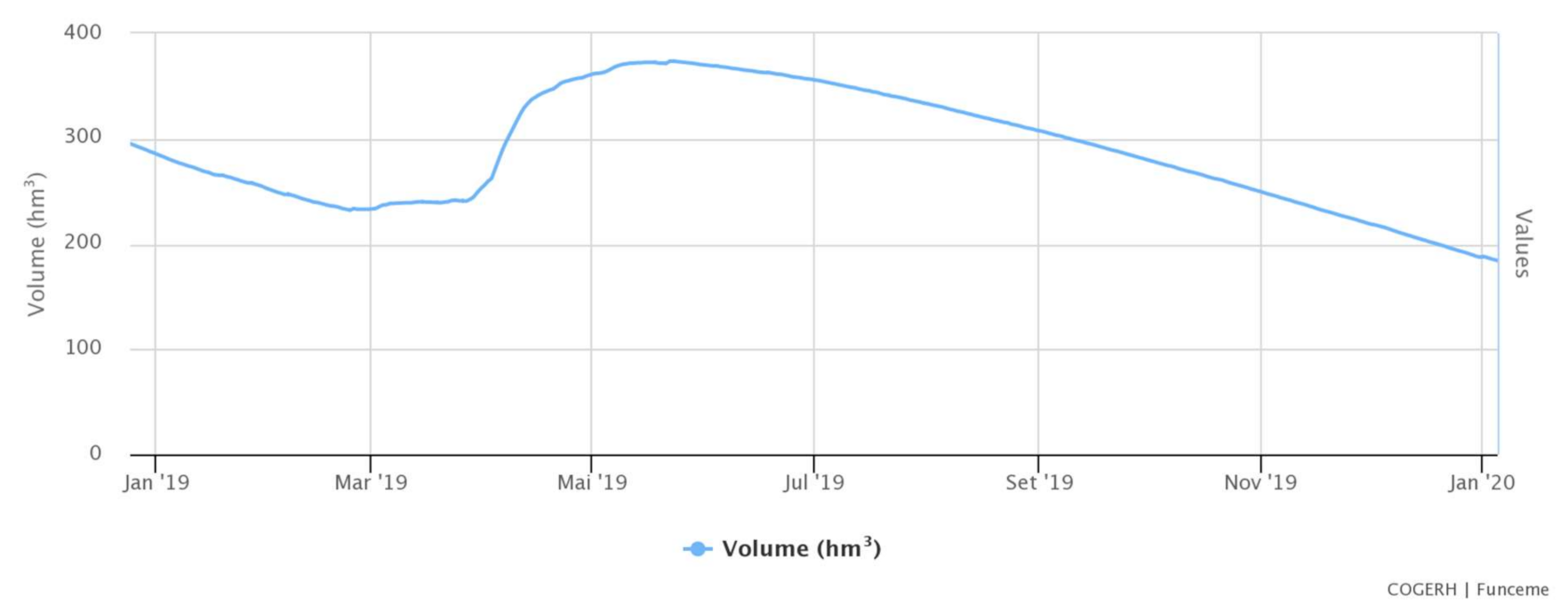
2.5. Hydroclimatic Data

Data on wind direction and wind speed, solar radiation and reservoir volume were used to generate a conceptual model to analyze the behavior of chl-a in surface waters of the Castanhão reservoir. This reservoir was chosen because, among the five reservoirs studied in this work, it presented a continuous monthly image sequence to estimate the concentration of chl-a using Sentinel-2 without cloud interference that could harm the understanding of the eutrophication cycle during a whole year, that is, for 2019.
For the wind data, a chart of the wind rose was generated, with the average of the values of the 4 days preceding the date of passage of the satellite, and at times of greatest gust (17:00, 18:00 and 19:00 LT; LT = local time = UTC-3:00). These peaks can be important because they control water column vertical mixing and resuspension of bottom sediment.
A graph was generated with the values of solar radiation in the days and times of the passage of the Sentinel-2 satellite (10:00 LT), to analyze the behavior of the concentration of chl-a against the possible thermal stratification of the column of water, generated by solar radiation incidence.
Daily variation of the water volume storage in the Castanhão reservoir was also retrieved, for the whole year 2019, to verify how water storage can interfere in the dilution or concentration of chl-a levels.

3. Results and Discussion

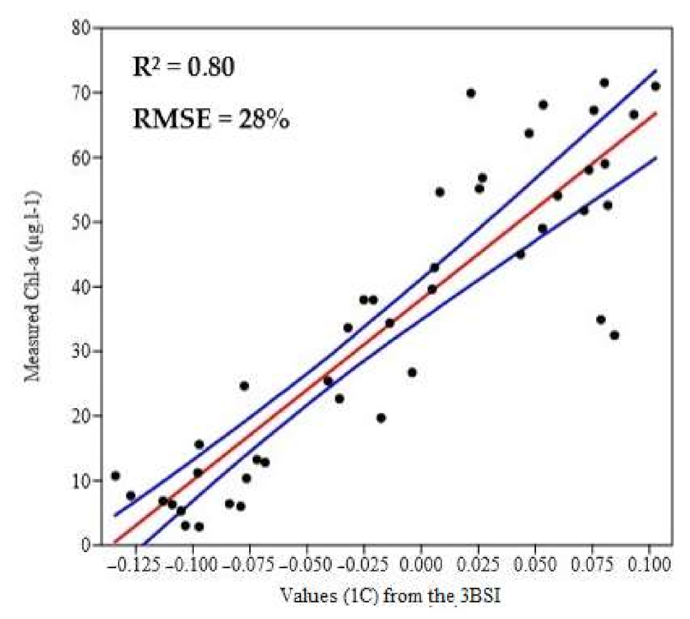
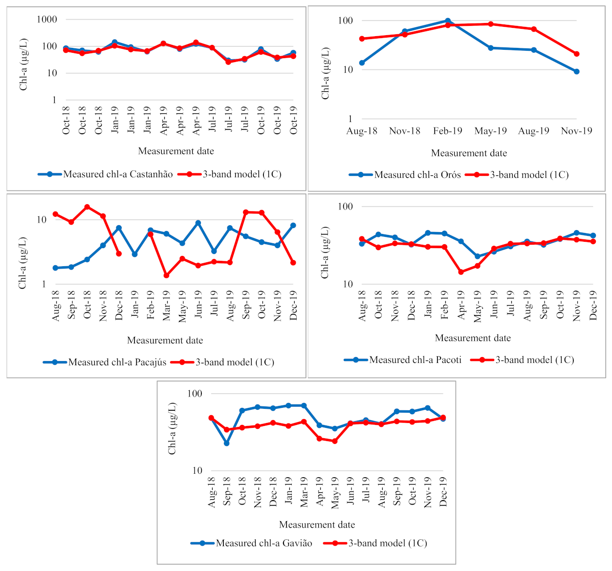
3.1. Chlorophyll-a Algorithm Definition and Performance

Table 2 shows the values of the chl-a samples collected in the 5 reservoirs considered in this work, from 2015 to 2018, used for calibration of the 3-band spectral model (Equation (1)). The datasets encompassed varying concentrations conditions. There was a strong variability in chl-a concentration from one reservoir to another, ranging from 0.2 to close to 90 µg L−1, and strong seasonality was also detected. The Pacajus reservoir showed a highly differentiated eutrophication pattern with low to intermediate concentration of chl-a [0.2–15.6 µg L−1].
The relationship between the chl-a concentration in the calibration dataset (Table 2) and the 3-band spectral index (Equation (1)) considering the spectral bands defined for Sentinel-2, R λ 1 = 665 nm; R λ 2 = 705 nm; and R λ 3 = 740 nm, obtained fine results with a a relative RMSE of 28% and R2 = 0.80. The calibrated chl-a model is:
Chl- a   ( µ g   L 1 ) = 279.95 3 BSI   +   38.06
From this chl-a retrieval algorithm, one can estimate the concentration of chl-a using Sentinel-2 Level 1C images.
Figure 2 shows the scatter plot of the values generated from the 3BSI for Sentinel-2 Level 1C images against the measured in situ calibration dataset.
The independent validation dataset was collected from August 2018 to December 2019. The estimated chl-a concentrations were compared to the observed chl-a concentrations (Figure 3). The correlation between the validation data, considering the 5 reservoirs, presented a coefficient of determination R2 = 0.77. Overall, the retrieved chl-a concentration followed well the temporal behavior of the field data except for the Pacajus reservoir, which presented the lowest chl-a concentration levels observed.
The difference in the performance of the algorithm for estimating low concentrations chl-a is probably related to the use of reflectance at λ3 in the three-band model because λ3 is practically insensitive to the absorption of water constituents (chl-a, CDOM and tripton), but is susceptible to suspended particle scattering (TSS). For low concentrations of chl-a, the correlation between backscatter and TSS increases considerably for longer wavelengths (λ3). This indicates an increased effect of the concentration of suspended particles. Thus, backscattering effects may not be fully removed using (λ3) and may introduce uncertainties in the concentrations chl-a estimation if the three-band model is applied. This can cause significant changes to the model output. Therefore, although the model has been calibrated for a wide range of biophysical and optical water quality parameters, the accuracy of the retrieval for a low chl-a concentration level (i.e., <10 µg L−1) may be considered with caution.
Figure 4 shows that chl-a concentration and turbidity (the latter is a proxy of scattering by phytoplankton and inorganic suspended matter) are not correlated (R2 < 0.09), denoting that that reservoir water presents complex behavior belonging clearly to case 2 waters.

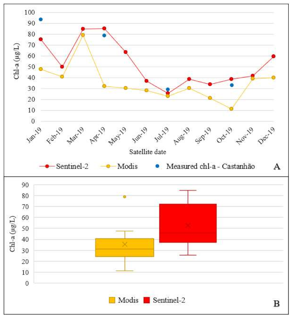
3.2. Chl-a Retrieval Comparison between Sentinel-2 and MODIS Sensors

We compared the chl-a time series retrieved with Sentinel-2 MSI sensor with an independent dataset based on MODIS (Terrra and Aqua satellites) available through the Hidrosat database (http://hidrosat.ana.gov.br/, accessed on 31 January 2022), developed by the Brazilian Water Agency (ANA) [117]. MODIS data offer higher sampling frequency than Sentinel 2 data with near daily acquisition rate. The Hidrosat database was calibrated using other field data and can be considered a totally independent dataset. Figure 5A presents the comparison between MODIS-derived and MSI-derived chl-a time series for 2019 over the Castanhão reservoir jointly to the field measurement already presented above. It can be seen that all datasets show close agreement, but some differences can be noticed during January, April, and October. It is worthwhile to note that the chl-a values assessed using Sentinel-2 are systematically closer to the field chl-adata, when compared to the values estimated by MODIS. The coarse resolution of MODIS data (i.e., 500 m) in relation to the 20-m Sentinel-2 data used for this study may partially explain this lower accuracy of the MODIS-derived estimates. Sentinel-2 images allow for greater refinement of the characteristics of the water body, reinforcing the gain in monitoring capacity and understanding of water quality processes in small and large reservoirs.
Figure 5B shows the distribution of both MODIS and Sentinel-2 derived chl-a data in a boxplot format. It is observed that the chl-a estimated by MODIS shows lower concentration values when compared to Sentinel-2 data. It is noteworthy that, in 2019, the Castanhão had its trophic status varying between hypereutrophic and eutrophic, as shown in Figure 6, which suggests a high chl-a concentration in that graph. In addition, Sentinel-2 has a greater range of concentration values throughout the year. That is more consistent with the field data collected in the reservoir, which showed greater chl-a concentration in the first months of the year, and a drop of concentration as the year goes by.

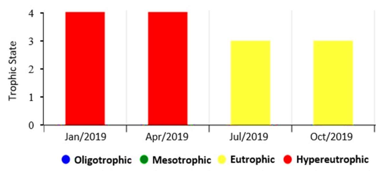
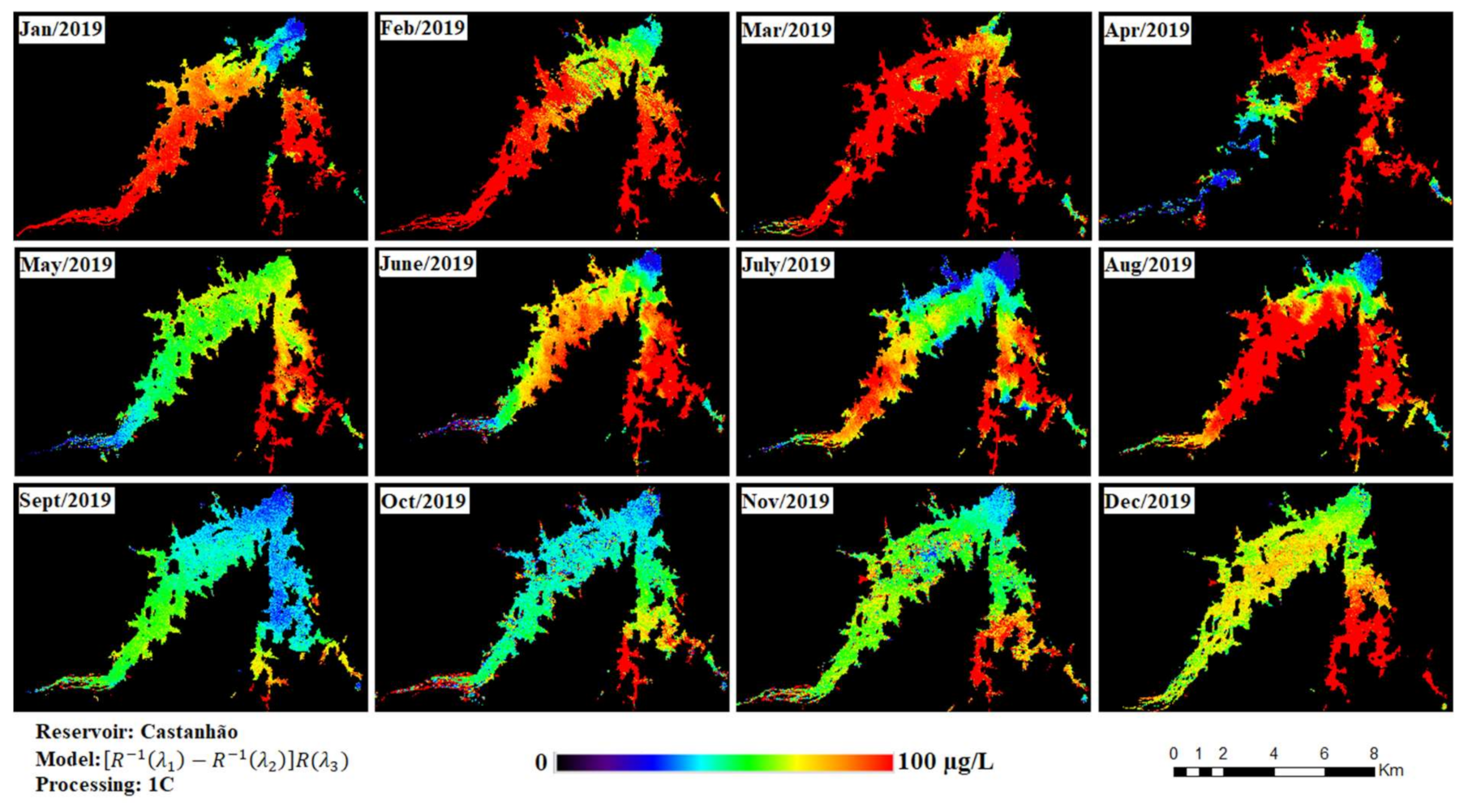
3.3. Analysis of the Trophic State Evolution in the Castanhão Reservoir

The trophic state graph, provided by COGERH, is presented (Figure 6) to compare and confirm the water quality results presented in the chl-a concentration maps (Figure 7) for the Castanhão reservoir during 2019.
The trophic state index used by COGERH to qualify the degree of trophy of the Ceará reservoirs is based on the proposal of [20] adapted by [21] to lentic environments of tropical climate. This index is based on chlorophyll-a and total phosphorus data. In other words, the greater the concentration of these parameters, the worse the water quality of aquatic environments will be.
For [21], in general, it is accepted that the trophic level of a water body can be evaluated from the chl-a concentration level alone.
Figure 7 shows the time series of the chl-a maps, generated for the Castanhão reservoir for every month of 2019 and prepared from Level 1C products, using Equation (2).
The chl-a concentration maps are consistent with the trophic state graph based on the in situ measurements (Figure 6) provided by COGERH. Figure 7 shows that between January and April the concentration of chl-a is high (i.e., >80 µg L−1) in a substantial part of the water body. In the following months, there is a decreasing chl-a concentration trend, indicating an improvement in the reservoir’s water quality, as shown in the trophic state graph (Figure 6), in which the Castanhão becomes eutrophic in the second half of the year. This can be explained by 1. Inflow: most of the inflow in 2019 concentrated in the months of April and May; 2. Reservoir volume: reduction in reservoir volume during the second semester since there is no inflow; 3. Wind speed: stronger winds starting in September, which promotes a better mixing of the reservoir waters. (As will be shown below.)
It is worth noting in the Sentinel-2 derived chl-a concentration maps (Figure 7) that the minimum chl-a concentration appears in the vicinity of the Castanhão dam, as shown in Figure 8, matching the deepest portion of the reservoir.
Figure 8, Figure 9 and Figure 10 show the variability of some hydroclimatic variables, namely reservoir volume, wind speed and direction, and solar radiation, respectively, to detect any relation with satellite-retrieved chl-a concentrations in the Castanhão reservoir, as shown in Figure 7. Temperature was not included in the analysis, as it varies little throughout the year in the study region, since it is close to the equator line, as well as relative humidity, which is mainly related to evaporation, and should have no effect on algal biomass development.
In the analyzed time scale, from a hydrodynamic point of view, the concentration of chl-a increases with the beginning of the rainy season in Ceará (March to May). This is probably because there are still no appreciable river water inputs from the upstream catchment, but there is a high input of nutrients by leaching and runoff from the baresoils areas around the dam. When the river starts to flow, a dilution effect is observed, with an increase in the volume of the reservoir and a simultaneous decrease in the concentration of chlorophyll. Thus, as shown in the estimated chl-a maps for the year 2019 (Figure 7), we can see a biomass dilution effect upstream of the reservoir (Figure 8), from April onwards, with the arrival of Jaguaribe River waters. In May there is a dilution of the biomass in most of the water mirror, due to the continuous increase in the volume of water in the reservoir, as a result of the rainy season in Ceará State. In June, as shown in Figure 9, the water volume starts to decrease as a result of the end of the rainy season, evaporation and multiple water uses. This decrease in the water volume matches an increase in the concentration of chl-a at the water surface. The analysis of the sequence of Sentinel-2-derived maps make it possible to monitor the rapid changes induced by the hydrological and meteorological conditions, confirming the strong control of these factors on the phytoplankton biomass in the Castanhão reservoir.
Figure 10 displays both wind intensity and mean direction for each month during 2019. It can be seen that there is a net increase in wind intensity from September to December. The analysis of the chl-a maps (Figure 7) shows a strong decrease in the values of chl-a in the entire surface of the Castanhão reservoir for the same period. This overall chl-a decrease at the lake surface may be directly related to both the wind speed increase and predominantly northeast direction from September to December 2019 (Figure 10) that generates a longitudinal turbulence in the reservoir mirror. It is worth highlighting the chl-a concentration in the month of August (Figure 7), as this month presents a more accentuated concentration compared to previous and following months. This concentration maximum may correspond to a combination of unique conditions with decreasing water storage at the beginning of the dry season, which corresponds to increasing water residence time and mild wind conditions.
From a meteorological point of view, the chlorophyll peak can occur simultaneously in the period of low wind speed. Wind can be an inducer of water mass movements, both horizontaly and spatially, and most phytoplankton species will not be able to develop. Furthermore, the action of the wind can cause sediment resuspension from the lake bottom, especially in shallow conditions when the reservoir faces low storage rate. This generates a lower availability of the light in the water column and may lead to inhibition of phytoplanktonic growth, resulting in lower chl-a concentrations values [77,79].
In this study, the radiation variability over the year did not seem to have a clear impact on chl-a variability at the surface level (Figure 11), since Castanhão is located close to the Equator and the solar irradiance is quite constant. Looking at finer time scales, both wind speed and radiation are closely related to the diurnal cycle of water quality: stratification of the reservoir during the peak of radiation and mixing of its water during the peak of the wind speed [118]. However, the study of the diurnal cycles remains out of the reach of the satellite date due to their lower time-revisit frequency.

4. Concluding Remarks

This work showed that the use of Sentinel-2 MSI remote-sensing data to monitor the quality of complex case 2 waters in semiarid environments has strong potential.
The defined 3-band spectral model for Sentinel-2 Level 1C, where R(λ1) = 665 nm; R(λ2) = 705 nm; and R(λ3) = 740 nm presented acceptable statistical performance to estimate the concentration of chl-a, with statistical regression parameters reaching a relative RMSE of 28% and R2 = 0.80.
The hydroclimatic data (wind direction and speed and reservoir volume) used to analyze the behavior of chl-a in the surface waters of the Castanhão reservoir was important, making it possible to interpret the temporal and spatial distribution of satellite-retrieved chl-a maps over the entire surface of the reservoir.
Thus, this study contributes to the development of continuous monitoring of water quality, based on remote analysis by satellite, in small and large reservoirs, a strategic resource to promote greater water security in the Brazilian semiarid region, which is heavily impacted by strong interannual rainfall variability and an overall scarcity of rainfall.

Author Contributions

Conceptualization, T.R.B.T.A.; Data curation, M.U.G.B.; Funding acquisition, E.S.P.R.M.; Supervision, J.-M.M.; Writing—review & editing, E.P.S. All authors have read and agreed to the published version of the manuscript.

Funding

The present work was carried out with the support of the Coordination for the Improvement of Higher Education Personnel—Brazil (CAPES)—Financing Code 001 in the context of the projects CNPq/490688/2010-1 and AQUASENSE/FINEP.

Data Availability Statement

Sentinel-2 satellite images are available on the website (https://scihub.copernicus.eu/, accessed on 14 January 2022); The estimated chl-a data for the Castanhão reservoir, through the MODIS satellite, are available on the website (http://hidrosat.ana.gov.br/, accessed on 14 January 2022); Data on chl-a collected in-situ are available at the Ceará Hydrological Portal (http://www.hidro.ce.gov.br/hidro-ce-zend/acude/eutrofizacao, accessed on 14 January 2022); Data on the volume of water in the Castanhão reservoir are also available on the Ceará Hydrological Portal (http://www.hidro.ce.gov.br/hidro-ce-zend/acude/nivel-diario, accessed on 14 January 2022); Brazilian National Institute of Meteorology data on wind direction and speed, and solar radiation are available at “https://portal.inmet.gov.br”, (accessed on 14 January 2022).

Acknowledgments

The first author is grateful to FUNCEME and CAPES for supporting her study.

Conflicts of Interest

The authors declare no conflict of interest.

References

  1. Teixeira, M.N. O Sertão Semiárido. Uma Relação de Sociedade e Natureza Numa Dinâmica de Organização Social Do Espaço. Soc. E Estado 2016, 31, 769–780. [Google Scholar] [CrossRef] [Green Version]
  2. de Araújo, J.C.; Güntner, A.; Bronstert, A. Loss of Reservoir Volume by Sediment Deposition and Its Impact on Water Availability in Semiarid Brazil. Hydrol. Sci. J. 2006, 51, 157–170. [Google Scholar] [CrossRef]
  3. de Araújo, J.C.; Döll, P.; Güntner, A.; Krol, M.; Abreu, C.B.R.; Hauschild, M.; Mendiondo, E.M. Water Scarcity under Scenarios for Global Climate Change and Regional Development in Semiarid Northeastern Brazil. Water Int. 2004, 29, 209–220. [Google Scholar] [CrossRef]
  4. Bucci, M.H.; De Oliveira, L.F.C. Índices de Qualidade Da Água e de Estado Trófico Na Represa Dr. João Penido (Juiz de Fora, MG). Ambiente E Agua—Interdiscip. J. Appl. Sci. 2014, 9, 243–251. [Google Scholar] [CrossRef]
  5. de Lucena Barbosa, J.E.; Medeiros, E.S.F.; Brasil, J.; da Silva Cordeiro, R.; Crispim, M.C.B.; da Silva, G.H.G. Aquatic Systems in Semi-Arid Brazil: Limnology and Management. Acta Limnol. Bras. 2012, 24, 103–118. [Google Scholar] [CrossRef]
  6. Pimenta, A.M.; Albertoni, E.F.; Palma-Silva, C. Characterization of Water Quality in a Small Hydropower Plant Reservoir in Southern Brazil. Lakes Reserv. Res. Manag. 2012, 17, 243–251. [Google Scholar] [CrossRef]
  7. Padisák, J.; Reynolds, C.S. Selection of Phytoplankton Associations in Lake Balaton, Hungary, in Response to Eutrophication and Restoration Measures, with Special Reference to the Cyanoprokaryotes. Hydrobiologia 1998, 384, 41–53. [Google Scholar] [CrossRef]
  8. Codd, G.A. Cyanobacterial Toxins, the Perception of Water Quality, and the Prioritisation of Eutrophication Control. Ecol. Eng. 2000, 16, 51–60. [Google Scholar] [CrossRef]
  9. Christoffersen, K.; Kaas, H. Toxic Cyanobacteria in Water. A Guide to Their Public Health Consequences, Monitoring, and Management. Limnol. Oceanogr. 2000, 45, 1212. [Google Scholar] [CrossRef]
  10. Sivonen, K. Cyanobacterial Toxins. In Encyclopedia of Microbiology; Elsevier: Amsterdam, The Netherlands, 2009; pp. 290–307. [Google Scholar]
  11. CARMICHAEL, W. The Cyanotoxins. In Incorporating in Plant Pathology—Classic Papers; Elsevier: Amsterdam, The Netherlands, 1997; Volume 27, pp. 211–256. ISBN 0-12-005927-4. [Google Scholar]
  12. Codd, G.A.; Ward, C.J.; Bell, S.G. Cyanobacterial Toxins: Occurrence, Modes of Action, Health Effects and Exposure Routes. Arch. Toxicol. Suppl. Arch. Für Toxikol. Suppl. 1997, 19, 399–410. [Google Scholar] [CrossRef]
  13. Hunter, P.R. Cyanobacterial Toxins and Human Health. J. Appl. Microbiol. Symp. Suppl. 1998, 84, 35–40. [Google Scholar] [CrossRef]
  14. Falconer, I.R. Health Problems from Exposure to Cyanobacteria and Proposed Safety Guidelines for Drinking and Recreational Water; The Royal Society of Chemistry: London, UK, 1994; p. 10. [Google Scholar]
  15. Kutser, T. Quantitative Detection of Chlorophyll in Cyanobacterial Blooms by Satellite Remote Sensing. Limnol. Oceanogr. 2004, 49, 2179–2189. [Google Scholar] [CrossRef]
  16. Richardson, L.L. Remote Sensing of Algal Bloom Dynamics. BioScience 1996, 46, 492–501. [Google Scholar] [CrossRef] [Green Version]
  17. Ross, M.R.V.; Topp, S.N.; Appling, A.P.; Yang, X.; Kuhn, C.; Butman, D.; Simard, M.; Pavelsky, T.M. AquaSat: A Data Set to Enable Remote Sensing of Water Quality for Inland Waters. Water Resour. Res. 2019, 55, 10012–10025. [Google Scholar] [CrossRef]
  18. Ha, N.T.T.; Koike, K.; Nhuan, M.T. Improved Accuracy of Chlorophyll-a Concentration Estimates from MODIS Imagery Using a Two-Band Ratio Algorithm and Geostatistics: As Applied to the Monitoring of Eutrophication Processes over Tien Yen Bay (Northern Vietnam). Remote Sens. 2013, 6, 421–442. [Google Scholar] [CrossRef] [Green Version]
  19. Markogianni, V.; Kalivas, D.; Petropoulos, G.P.; Dimitriou, E. Estimating Chlorophyll-a of Inland Water Bodies in Greece Based on Landsat Data. Remote Sens. 2020, 12, 2087. [Google Scholar] [CrossRef]
  20. Carlson, R.E. A Trophic State Index for Lakes. Limnol. Oceanogr. 1977, 22, 361–369. [Google Scholar] [CrossRef] [Green Version]
  21. Toledo Júnior, A.P.; Talarico, M.; Chinez, S.J.; Agudo, E.G.A. A Aplicação de Modelos Simplificados Para a Avaliação de Processo Da Eutrofização Em Lagos e Reservatórios Tropicais. In Proceedings of the Congresso Brasileiro de Engenharia Sanitária, Camboriú, Brazil, 20–25 November 1983. [Google Scholar]
  22. Halstvedt, C.B.; Rohrlack, T.; Andersen, T.; Skulberg, O.; Edvardsen, B. Seasonal Dynamics and Depth Distribution of Planktothrix Spp. in Lake Steinsfjorden (Norway) Related to Environmental Factors. J. Plankton Res. 2007, 29, 471–482. [Google Scholar] [CrossRef] [Green Version]
  23. Reynolds, C.S.; Oliver, R.L.; Walsby, A.E. Cyanobacterial Dominance: The Role of Buoyancy Regulation in Dynamic Lake Environments. N. Z. J. Mar. Freshw. Res. 1987, 21, 379–390. [Google Scholar] [CrossRef]
  24. Walsby, A.E.; Hayes, P.K.; Boje, R.; Stal, L.J. The Selective Advantage of Buoyancy Provided by Gas Vesicles for Planktonic Cyanobacteria in the Baltic Sea. New Phytol. 1997, 136, 407–417. [Google Scholar] [CrossRef]
  25. Pitois, S.; Jackson, M.H.; Wood, B.J.B. Problems Associated with the Presence of Cyanobacteria in Recreational and Drinking Waters. Int. J. Environ. Health Res. 2000, 10, 203–218. [Google Scholar] [CrossRef]
  26. Backer, L.C. Cyanobacterial Harmful Algal Blooms (CyanoHABs): Developing a Public Health Response. Lake Reserv. Manag. 2002, 18, 20–31. [Google Scholar] [CrossRef]
  27. Johansen, R.; Beck, R.; Nowosad, J.; Nietch, C.; Xu, M.; Shu, S.; Yang, B.; Liu, H.; Emery, E.; Reif, M.; et al. Evaluating the Portability of Satellite Derived Chlorophyll-a Algorithms for Temperate Inland Lakes Using Airborne Hyperspectral Imagery and Dense Surface Observations. Harmful Algae 2018, 76, 35–46. [Google Scholar] [CrossRef] [PubMed]
  28. Neil, C.; Spyrakos, E.; Hunter, P.D.; Tyler, A.N. A Global Approach for Chlorophyll-a Retrieval across Optically Complex Inland Waters Based on Optical Water Types. Remote Sens. Environ. 2019, 229, 159–178. [Google Scholar] [CrossRef]
  29. Pahlevan, N.; Lee, Z.; Wei, J.; Schaaf, C.B.; Schott, J.R.; Berk, A. On-Orbit Radiometric Characterization of OLI (Landsat-8) for Applications in Aquatic Remote Sensing. Remote Sens. Environ. 2014, 154, 272–284. [Google Scholar] [CrossRef]
  30. Tavares, M.H.; Lins, R.C.; Harmel, T.; Fragoso, C.R.; Martínez, J.M.; Motta-Marques, D. Atmospheric and Sunglint Correction for Retrieving Chlorophyll-a in a Productive Tropical Estuarine-Lagoon System Using Sentinel-2 MSI Imagery. ISPRS J. Photogramm. Remote Sens. 2021, 174, 215–236. [Google Scholar] [CrossRef]
  31. Dörnhöfer, K.; Oppelt, N. Remote Sensing for Lake Research and Monitoring—Recent Advances. Ecol. Indic. 2016, 64, 105–122. [Google Scholar] [CrossRef]
  32. Hedley, J.; Roelfsema, C.; Koetz, B.; Phinn, S. Capability of the Sentinel 2 Mission for Tropical Coral Reef Mapping and Coral Bleaching Detection. Remote Sens. Environ. 2012, 120, 145–155. [Google Scholar] [CrossRef]
  33. Bresciani, M.; Cazzaniga, I.; Austoni, M.; Sforzi, T.; Buzzi, F.; Morabito, G.; Giardino, C. Mapping Phytoplankton Blooms in Deep Subalpine Lakes from Sentinel-2A and Landsat-8. Hydrobiologia 2018, 824, 197–214. [Google Scholar] [CrossRef] [Green Version]
  34. Dekker, A.G.; Brando, V.E.; Anstee, J.M.; Pinnel, N.; Kutser, T.; Hoogenboom, E.J.; Peters, S.; Pasterkamp, R.; Vos, R.; Olbert, C.; et al. Imaging Spectrometry of Water. In Imaging Spectrometry; Springer: Berlin/Heidelberg, Germany, 2002; pp. 307–359. [Google Scholar] [CrossRef]
  35. Gholizadeh, M.H.; Melesse, A.M.; Reddi, L. A Comprehensive Review on Water Quality Parameters Estimation Using Remote Sensing Techniques. Sensors 2016, 16, 1298. [Google Scholar] [CrossRef] [Green Version]
  36. Odermatt, D.; Gitelson, A.; Brando, V.E.; Schaepman, M. Review of Constituent Retrieval in Optically Deep and Complex Waters from Satellite Imagery. Remote Sens. Environ. 2012, 118, 116–126. [Google Scholar] [CrossRef] [Green Version]
  37. Kupssinskü, L.S.; Guimarães, T.T.; De Souza, E.M.; Zanotta, D.C.; Veronez, M.R.; Gonzaga, L.; Mauad, F.F. A Method for Chlorophyll-a and Suspended Solids Prediction through Remote Sensing and Machine Learning. Sensors 2020, 20, 2125. [Google Scholar] [CrossRef] [Green Version]
  38. Sun, D.; Li, Y.; Wang, Q.; Le, C.; Lv, H.; Huang, C.; Gong, S. Specific Inherent Optical Quantities of Complex Turbid Inland Waters, from the Perspective of Water Classification. Photochem. Photobiol. Sci. 2012, 11, 1299–1312. [Google Scholar] [CrossRef] [PubMed]
  39. Ma, J.; Song, K.; Wen, Z.; Zhao, Y.; Shang, Y.; Fang, C.; Du, J. Spatial Distribution of Diffuse Attenuation of Photosynthetic Active Radiation and Its Main Regulating Factors in Inland Waters of Northeast China. Remote Sens. 2016, 8, 964. [Google Scholar] [CrossRef] [Green Version]
  40. Lisboa, F.; Brotas, V.; Santos, F.D.; Kuikka, S.; Kaikkonen, L.; Maeda, E.E. Spatial Variability and Detection Levels for Chlorophyll-a Estimates in High Latitude Lakes Using Landsat Imagery. Remote Sens. 2020, 12, 2898. [Google Scholar] [CrossRef]
  41. Soomets, T.; Uudeberg, K.; Kangro, K.; Jakovels, D.; Brauns, A.; Toming, K.; Zagars, M.; Kutser, T. Spatio-Temporal Variability of Phytoplankton Primary Production in Baltic Lakes Using Sentinel-3 OLCI Data. Remote Sens. 2020, 12, 2415. [Google Scholar] [CrossRef]
  42. Gitelson, A. The Peak near 700 Nm on Radiance Spectra of Algae and Water: Relationships of Its Magnitude and Position with Chlorophyll Concentration. Int. J. Remote Sens. 1992, 13, 3367–3373. [Google Scholar] [CrossRef]
  43. Gitelson, A.; Mayo, M.; Yacobi, Y.Z.; Parparov, A.; Berman, T. The Use of High-Spectral-Resolution Radiometer Data for Detection of Low Chlorophyll Concentrations in Lake Kinneret. J. Plankton Res. 1994, 16, 993–1002. [Google Scholar] [CrossRef]
  44. Jensen, J.R. Sensoriamento Remoto Do Ambiente: Uma Perspectiva Em Recursos Terrestres; Tradução 2; Epiphanio, J.C.N., Formaggio, A.R., Santos, A.R., Rudorff, B.F.T., Almeida, C.M., Galvão, L.S., Eds.; Parêntese: São José dos Campos, Brazil, 2009; p. 672. ISBN 978-85-60507-06-1. [Google Scholar]
  45. Le, C.; Li, Y.; Zha, Y.; Wang, Q.; Zhang, H.; Yin, B. Remote Sensing of Phycocyanin Pigment in Highly Turbid Inland Waters in Lake Taihu, China. Int. J. Remote Sens. 2011, 32, 8253–8269. [Google Scholar] [CrossRef]
  46. Matthews, M.W.; Bernard, S.; Robertson, L. An Algorithm for Detecting Trophic Status (Chlorophyll-a), Cyanobacterial-Dominance, Surface Scums and Floating Vegetation in Inland and Coastal Waters. Remote Sens. Environ. 2012, 124, 637–652. [Google Scholar] [CrossRef]
  47. Heisler, J.; Glibert, P.M.; Burkholder, J.M.; Anderson, D.M.; Cochlan, W.; Dennison, W.C.; Dortch, Q.; Gobler, C.J.; Heil, C.A.; Humphries, E.; et al. Eutrophication and Harmful Algal Blooms: A Scientific Consensus. Harmful Algae 2008, 8, 3–13. [Google Scholar] [CrossRef] [PubMed] [Green Version]
  48. de Castro Medeiros, L.; Mattos, A.; Lürling, M.; Becker, V. Is the Future Blue-Green or Brown? The Effects of Extreme Events on Phytoplankton Dynamics in a Semi-Arid Man-Made Lake. Aquat. Ecol. 2015, 49, 293–307. [Google Scholar] [CrossRef]
  49. Kangur, K.; Möls, T.; Milius, A.; Laugaste, R. Phytoplankton Response to Changed Nutrient Level in Lake Peipsi (Estonia) in 1992-2001. Hydrobiologia 2003, 506–509, 265–272. [Google Scholar] [CrossRef]
  50. Naselli-Flores, L.; Barone, R. Water-Level Fluctuations in Mediterranean Reservoirs: Setting a Dewatering Threshold as a Management Tool to Improve Water Quality. Hydrobiologia 2005, 548, 85–99. [Google Scholar] [CrossRef]
  51. Leira, M.; Cantonati, M. Effects of Water-Level Fluctuations on Lakes: An Annotated Bibliography. Hydrobiologia 2008, 613, 171–184. [Google Scholar] [CrossRef]
  52. Geraldes, A.M.; Boavida, M.J. Zooplankton Assemblages in Two Reservoirs: One Subjected to Accentuated Water Level Fluctuations, the Other with More Stable Water Levels. Aquat. Ecol. 2007, 41, 273–284. [Google Scholar] [CrossRef] [Green Version]
  53. Naselli-Flores, L. Morphological Analysis of Phytoplankton as a Tool to Assess Ecological State of Aquatic Ecosystems: The Case of Lake Arancio, Sicily, Italy. Inland Waters 2014, 4, 15–26. [Google Scholar] [CrossRef] [Green Version]
  54. Reynolds, C.S. The Ecology of Phytoplankton (Ecology, Biodiversity and Conservation); Cambridge University Press: Cambridge, UK, 2006. [Google Scholar]
  55. Soares, M.C.S.; Marinho, M.M.; Azevedo, S.M.O.F.; Branco, C.W.C.; Huszar, V.L.M. Eutrophication and Retention Time Affecting Spatial Heterogeneity in a Tropical Reservoir. Limnologica 2012, 42, 197–203. [Google Scholar] [CrossRef]
  56. da Costa, M.R.A.; Attayde, J.L.; Becker, V. Effects of Water Level Reduction on the Dynamics of Phytoplankton Functional Groups in Tropical Semi-Arid Shallow Lakes. Hydrobiologia 2016, 778, 75–89. [Google Scholar] [CrossRef]
  57. Naselli-flores, L. Man-Made Lakes in Mediterranean Semi-Arid Climate: The Strange Case of Dr Deep Lake and Mr Shallow Lake. Hydrobiologia 2003, 506, 13–21. [Google Scholar] [CrossRef]
  58. Geraldes, A.M.; Boavida, M.J. Seasonal Water Level Fluctuations: Implications for Reservoir Limnology and Management. Lakes Reserv. Res. Manag. 2005, 10, 59–69. [Google Scholar] [CrossRef] [Green Version]
  59. Bond, N.R.; Lake, P.S.; Arthington, A.H. The Impacts of Drought on Freshwater Ecosystems: An Australian Perspective. Hydrobiologia 2008, 600, 3–16. [Google Scholar] [CrossRef] [Green Version]
  60. Özen, A.; Karapinar, B.; Kucuk, I.; Jeppesen, E.; Beklioglu, M. Drought-Induced Changes in Nutrient Concentrations and Retention in Two Shallow Mediterranean Lakes Subjected to Different Degrees of Management. Hydrobiologia 2010, 646, 61–72. [Google Scholar] [CrossRef]
  61. Teferi, M.; Declerck, S.; Lemmens, P.; Gebrekidan, A. Strong Effects of Occasional Drying on Subsequent Water Clarity and Cyanobacterial Blooms in Cool Tropical Reservoirs. Freshw. Biol. 2014, 59, 870–884. [Google Scholar] [CrossRef] [Green Version]
  62. Braga, G.G.; Becker, V.; Neuciano Pinheiro de Oliveira, J.; Rodrigues de Mendonça Junior, J.; Felipe de Medeiros Bezerra, A.; Macêdo Torres, L.; Marília Freitas Galvão, Â.; Mattos, A. Influence of Extended Drought on Water Quality in Tropical Reservoirs in a Semiarid Region. Acta Limnol. Bras. 2015, 27, 15–23. [Google Scholar] [CrossRef] [Green Version]
  63. Jeppesen, E.; Brucet, S.; Naselli-Flores, L.; Papastergiadou, E.; Stefanidis, K.; Nõges, T.; Nõges, P.; Attayde, J.L.; Zohary, T.; Coppens, J.; et al. Ecological Impacts of Global Warming and Water Abstraction on Lakes and Reservoirs Due to Changes in Water Level and Related Changes in Salinity. Hydrobiologia 2015, 750, 201–227. [Google Scholar] [CrossRef]
  64. do Vale Figueiredo, A.; Becker, V. Influence of Extreme Hydrological Events in the Quality of Water Reservoirs in the Semi-Arid Tropical Region. RBRH 2018, 23, 1–8. [Google Scholar] [CrossRef]
  65. Kosten, S.; Huszar, V.L.M.; Bécares, E.; Costa, L.S.; van Donk, E.; Hansson, L.A.; Jeppesen, E.; Kruk, C.; Lacerot, G.; Mazzeo, N.; et al. Warmer Climates Boost Cyanobacterial Dominance in Shallow Lakes. Glob. Change Biol. 2012, 18, 118–126. [Google Scholar] [CrossRef]
  66. Romo, S.; Soria, J.; Fernández, F.; Ouahid, Y.; Barón-Solá, Á. Water Residence Time and the Dynamics of Toxic Cyanobacteria. Freshw. Biol. 2013, 58, 513–522. [Google Scholar] [CrossRef]
  67. Wagner, C.; Adrian, R. Cyanobacteria Dominance: Quantifying the Effects of Climate Change. Limnol. Oceanogr. 2009, 54, 2460–2468. [Google Scholar] [CrossRef]
  68. Willis, A.; Chuang, A.W.; Orr, P.T.; Beardall, J.; Burford, M.A. Subtropical Freshwater Phytoplankton Show a Greater Response to Increased Temperature than to Increased PCO2. Harmful Algae 2019, 90, 101705. [Google Scholar] [CrossRef] [PubMed]
  69. Accoroni, S.; Ceci, M.; Tartaglione, L.; Romagnoli, T.; Campanelli, A.; Marini, M.; Giulietti, S.; Dell’Aversano, C.; Totti, C. Role of Temperature and Nutrients on the Growth and Toxin Production of Prorocentrum Hoffmannianum (Dinophyceae) from the Florida Keys. Harmful Algae 2018, 80, 140–148. [Google Scholar] [CrossRef]
  70. Gobler, C.J. Climate Change and Harmful Algal Blooms: Insights and Perspective. Harmful Algae 2020, 91, 101731. [Google Scholar] [CrossRef] [PubMed]
  71. Liu, X.; Lu, X.; Chen, Y. The Effects of Temperature and Nutrient Ratios on Microcystis Blooms in Lake Taihu, China: An 11-Year Investigation. Harmful Algae 2011, 10, 337–343. [Google Scholar] [CrossRef]
  72. Paerl, H.W.; Huisman, J. Climate: Blooms like It Hot. Science 2008, 320, 57–58. [Google Scholar] [CrossRef] [Green Version]
  73. Peperzak, L. Climate Change and Harmful Algal Blooms in the North Sea. Acta Oecologica 2003, 24, S139–S144. [Google Scholar] [CrossRef]
  74. Paerl, H.W.; Huisman, J. Climate Change: A Catalyst for Global Expansion of Harmful Cyanobacterial Blooms. Environ. Microbiol. Rep. 2009, 1, 27–37. [Google Scholar] [CrossRef]
  75. O’Neil, J.M.; Davis, T.W.; Burford, M.A.; Gobler, C.J. The Rise of Harmful Cyanobacteria Blooms: The Potential Roles of Eutrophication and Climate Change. Harmful Algae 2012, 14, 313–334. [Google Scholar] [CrossRef]
  76. Allende, L.; Tell, G.; Zagarese, H.; Torremorell, A.; Pérez, G.; Bustingorry, J.; Escaray, R.; Izaguirre, I. Phytoplankton and Primary Production in Clear-Vegetated, Inorganic-Turbid, and Algal-Turbid Shallow Lakes from the Pampa Plain (Argentina). Hydrobiologia 2009, 624, 45–60. [Google Scholar] [CrossRef]
  77. Feng, L.; Chen, B.; Hayat, T.; Alsaedi, A.; Ahmad, B. Modelling the Influence of Thermal Discharge under Wind on Algae. Phys. Chem. Earth 2015, 79–82, 108–114. [Google Scholar] [CrossRef]
  78. Xia, M.; Jiang, L. Influence of Wind and River Discharge on the Hypoxia in a Shallow Bay. Ocean Dyn. 2015, 65, 665–678. [Google Scholar] [CrossRef]
  79. Zhang, Y.; Loiselle, S.; Shi, K.; Han, T.; Zhang, M.; Hu, M.; Jing, Y.; Lai, L.; Zhan, P. Wind Effects for Floating Algae Dynamics in Eutrophic Lakes. Remote Sens. 2021, 13, 800. [Google Scholar] [CrossRef]
  80. Governo do Estado do Ceará. Portal Hidrológico Do Ceará. Tabela Detalhamento Açudes. Available online: http://www.hidro.ce.gov.br/ (accessed on 8 January 2022).
  81. Molisani, M.M.; Becker, H.; Barroso, H.S.; Hijo, C.A.G.; Monte, T.M.; Vasconcellos, G.H.; Lacerda, L.D. The Influence of Castanhão Reservoir on Nutrient and Suspended Matter Transport during Rainy Season in the Ephemeral Jaguaribe River (CE, Brazil). Braz. J. Biol. 2013, 73, 115–123. [Google Scholar] [CrossRef] [PubMed] [Green Version]
  82. Alves, J.M.B.; Campos, J.N.B.; Servain, J. Reservoir Management Using Coupled Atmospheric and Hydrological Models: The Brazilian Semi-Arid Case. Water Resour. Manag. 2012, 26, 1365–1385. [Google Scholar] [CrossRef]
  83. dos Santos, J.C.N.; de Andrade, E.M.; de Araújo Neto, J.R.; Meireles, A.C.M.; de Queiroz Palácio, H.A. Land Use and Trophic State Dynamics in a Tropical Semi-Arid Reservoir. Rev. Cienc. Agron. 2014, 45, 35–44. [Google Scholar] [CrossRef] [Green Version]
  84. Medeiros, P.H.A.; de Araújo, J.C.; Bronstert, A. Medidas de Interceptação e Avaliação Do Desempenho Do Modelo de Gash Para Uma Região Semi-Árida. Rev. Cienc. Agron. 2009, 40, 165–174. [Google Scholar]
  85. Lima Neto, I.E.; Wiegand, M.C.; Carlos de Araújo, J. Redistribution Des Sédiments Due à Un Réseau Dense de Réservoirs Dans Un Grand Bassin Versant Semi-Aride Du Brésil. Hydrol. Sci. J. 2011, 56, 319–333. [Google Scholar] [CrossRef]
  86. Campos, J.N.B.; Souza Filho, F.A.; Lima, H.V.C. Risques et Incertitudes de Rendement de Réservoir Dans Des Riviéres Intermittentes Trés Variables: Cas Du Réservoir Castanhão Dans Le Brésil Semi-Aride. Hydrol. Sci. J. 2014, 59, 1184–1195. [Google Scholar] [CrossRef]
  87. Pereira, B.; Medeiros, P.; Francke, T.; Ramalho, G.; Foerster, S.; De Araújo, J.C. Assessment of the Geometry and Volumes of Small Surface Water Reservoirs by Remote Sensing in a Semi-Arid Region with High Reservoir Density. Hydrol. Sci. J. 2019, 64, 66–79. [Google Scholar] [CrossRef]
  88. Barros, M.U.G.; Wilson, A.E.; Leitão, J.I.R.; Pereira, S.P.; Buley, R.P.; Fernandez-Figueroa, E.G.; Capelo-Neto, J. Environmental Factors Associated with Toxic Cyanobacterial Blooms across 20 Drinking Water Reservoirs in a Semi-Arid Region of Brazil. Harmful Algae 2019, 86, 128–137. [Google Scholar] [CrossRef]
  89. Palmer, S.C.J.; Kutser, T.; Hunter, P.D. Remote Sensing of Inland Waters: Challenges, Progress and Future Directions. Remote Sens. Environ. 2015, 157, 1–8. [Google Scholar] [CrossRef] [Green Version]
  90. Kallio, K.; Attila, J.; Härmä, P.; Koponen, S.; Pulliainen, J.; Hyytiäinen, U.M.; Pyhälahti, T. Landsat ETM+ Images in the Estimation of Seasonal Lake Water Quality in Boreal River Basins. Environ. Manage. 2008, 42, 511–522. [Google Scholar] [CrossRef] [PubMed]
  91. Kutser, T.; Paavel, B.; Verpoorter, C.; Ligi, M.; Soomets, T.; Toming, K.; Casal, G. Remote Sensing of Black Lakes and Using 810 Nm Reflectance Peak for Retrieving Water Quality Parameters of Optically Complex Waters. Remote Sens. 2016, 8, 497. [Google Scholar] [CrossRef]
  92. Toming, K.; Kutser, T.; Laas, A.; Sepp, M.; Paavel, B.; Nõges, T. First Experiences in Mapping Lakewater Quality Parameters with Sentinel-2 MSI Imagery. Remote Sens. 2016, 8, 640. [Google Scholar] [CrossRef] [Green Version]
  93. Rice, E.W.; Bridgewater, L. Standard Methods for the Examination of Water and Wastewater; Rice, E.W., Ed.; American Public Health Association, American Water Works Association, Water Environment Federation: Washington, DC, USA, 2012; ISBN 978-0-87553-013-0. [Google Scholar]
  94. Hijo, C.A.G. Quantificação Do Efeito Do Açude Castanhão Sobre o Fluxo Fluvial de Material Particulado Em Suspensão e Nutrientes Para o Estuário Do Rio Jaguaribe, Ceará—Brasil. Master’s Thesis, Universidade Federal do Ceará, Fortaleza, Brazil, 2009. [Google Scholar]
  95. Bouvy, M.; Molica, R.; De Oliveira, S.; Marinho, M.; Beker, B. Dynamics of a Toxic Cyanobacterial Bloom (Cylindrospermopsis Raciborskii) in a Shallow Reservoir in the Semi-Arid Region of Northeast Brazil. Aquat. Microb. Ecol. 1999, 20, 285–297. [Google Scholar] [CrossRef] [Green Version]
  96. Schroeder, T.; Behnert, I.; Schaale, M.; Fischer, J.; Doerffer, R. Atmospheric Correction Algorithm for MERIS above Case-2 Waters. Int. J. Remote Sens. 2007, 28, 1469–1486. [Google Scholar] [CrossRef]
  97. Topp, S.N.; Pavelsky, T.M.; Jensen, D.; Simard, M.; Ross, M.R.V. Research Trends in the Use of Remote Sensing for Inland Water Quality Science: Moving towards Multidisciplinary Applications. Water 2020, 12, 169. [Google Scholar] [CrossRef] [Green Version]
  98. Jamet, C.; Loisel, H.; Kuchinke, C.P.; Ruddick, K.; Zibordi, G.; Feng, H. Comparison of Three SeaWiFS Atmospheric Correction Algorithms for Turbid Waters Using AERONET-OC Measurements. Remote Sens. Environ. 2011, 115, 1955–1965. [Google Scholar] [CrossRef]
  99. Matthews, M.W.; Odermatt, D. Improved Algorithm for Routine Monitoring of Cyanobacteria and Eutrophication in Inland and Near-Coastal Waters. Remote Sens. Environ. 2015, 156, 374–382. [Google Scholar] [CrossRef]
  100. Soriano-González, J.; Angelats, E.; Fernández-Tejedor, M.; Diogene, J.; Alcaraz, C. First Results of Phytoplankton Spatial Dynamics in Two NW-Mediterranean Bays from Chlorophyll-A Estimates Using Sentinel 2: Potential Implications for Aquaculture. Remote Sens. 2019, 11, 1756. [Google Scholar] [CrossRef] [Green Version]
  101. Dall’Olmo, G.; Gitelson, A.A. Effect of Bio-Optical Parameter Variability on the Remote Estimation of Chlorophyll-a Concentration in Turbid Productive Waters: Experimental Results. Appl. Opt. 2005, 44, 412. [Google Scholar] [CrossRef] [PubMed] [Green Version]
  102. Gitelson, A.A.; Dall’Olmo, G.; Moses, W.; Rundquist, D.C.; Barrow, T.; Fisher, T.R.; Gurlin, D.; Holz, J. A Simple Semi-Analytical Model for Remote Estimation of Chlorophyll-a in Turbid Waters: Validation. Remote Sens. Environ. 2008, 112, 3582–3593. [Google Scholar] [CrossRef]
  103. Sun, D.; Li, Y.; Wang, Q. A Unified Model for Remotely Estimating Chlorophyll a in Lake Taihu, China, Based on SVM and in Situ Hyperspectral Data. IEEE Trans. Geosci. Remote Sens. 2009, 47, 2957–2965. [Google Scholar] [CrossRef]
  104. Hunter, P.D.; Tyler, A.N.; Carvalho, L.; Codd, G.A.; Maberly, S.C. Hyperspectral Remote Sensing of Cyanobacterial Pigments as Indicators for Cell Populations and Toxins in Eutrophic Lakes. Remote Sens. Environ. 2010, 114, 2705–2718. [Google Scholar] [CrossRef] [Green Version]
  105. Mishra, S.; Mishra, D.R. Normalized Difference Chlorophyll Index: A Novel Model for Remote Estimation of Chlorophyll-a Concentration in Turbid Productive Waters. Remote Sens. Environ. 2012, 117, 394–406. [Google Scholar] [CrossRef]
  106. Lyu, H.; Li, X.; Wang, Y.; Jin, Q.; Cao, K.; Wang, Q.; Li, Y. Evaluation of Chlorophyll-a Retrieval Algorithms Based on MERIS Bands for Optically Varying Eutrophic Inland Lakes. Sci. Total Environ. 2015, 530–531, 373–382. [Google Scholar] [CrossRef]
  107. Shanmugam, P.; He, X.; Singh, R.K.; Varunan, T. A Modern Robust Approach to Remotely Estimate Chlorophyll in Coastal and Inland Zones. Adv. Space Res. 2018, 61, 2491–2509. [Google Scholar] [CrossRef]
  108. Moses, W.J.; Saprygin, V.; Gerasyuk, V.; Povazhnyy, V.; Berdnikov, S.; Gitelson, A.A. OLCI-Based NIR-Red Models for Estimating Chlorophyll- a Concentration in Productive Coastal Waters—a Preliminary Evaluation. Environ. Res. Commun. 2019, 1, 011002. [Google Scholar] [CrossRef]
  109. Van Nguyen, M.; Lin, C.H.; Chu, H.J.; Jaelani, L.M.; Syariz, M.A. Spectral Feature Selection Optimization for Water Quality Estimation. Int. J. Environ. Res. Public. Health 2020, 17, 272. [Google Scholar] [CrossRef] [Green Version]
  110. Ogashawara, I.; Kiel, C.; Jechow, A.; Kohnert, K.; Ruhtz, T.; Grossart, H.P.; Hölker, F.; Nejstgaard, J.C.; Berger, S.A.; Wollrab, S. The Use of Sentinel-2 for Chlorophyll-A Spatial Dynamics Assessment: A Comparative Study on Different Lakes in Northern Germany. Remote Sens. 2021, 13, 1542. [Google Scholar] [CrossRef]
  111. Zimba, P.V.; Gitelson, A. Remote Estimation of Chlorophyll Concentration in Hyper-Eutrophic Aquatic Systems: Model Tuning and Accuracy Optimization. Aquaculture 2006, 256, 272–286. [Google Scholar] [CrossRef]
  112. Gurlin, D.; Gitelson, A.A.; Moses, W.J. Remote Estimation of Chl-a Concentration in Turbid Productive Waters—Return to a Simple Two-Band NIR-Red Model? Remote Sens. Environ. 2011, 115, 3479–3490. [Google Scholar] [CrossRef]
  113. Kutser, T. The Possibility of Using the Landsat Image Archive for Monitoring Long Time Trends in Coloured Dissolved Organic Matter Concentration in Lake Waters. Remote Sens. Environ. 2012, 123, 334–338. [Google Scholar] [CrossRef]
  114. Cardille, J.A.; Leguet, J.B.; del Giorgio, P. Remote Sensing of Lake CDOM Using Noncontemporaneous Field Data. Can. J. Remote Sens. 2013, 39, 118–126. [Google Scholar] [CrossRef]
  115. Efron, B. Bootstrap Methods: Another Look at the Jackknife. Ann. Stat. 1979, 7, 1–26. [Google Scholar] [CrossRef]
  116. de Almeida, R.M.V.R.; Infantosi, A.F.C.; Gismondi, R.C. Replicação Bootstrap e Análise de Sensibilidade Em Redes Neurais Artificiais. In Proceedings of the Anais do 5. Congresso Brasileiro de Redes Neurais, Rio de Janeiro, Brazil, 2–5 April 2001; pp. 295–300. [Google Scholar]
  117. Martinez, J.M.; Ventura, D.; Cochonneau, G.; De Oliveira, E.; Cerqueira Piscoya, R.; Santos Guimarães, V. Monitoring of Water Quality and Water Level of Rivers and Lakes in Brazil: Towards a Remote Sensing-Based Operational Monitoring Application at the Brazilian National Water Agency. In Applications of Satellite Earth Observations: Serving Society, Science & Industry; CEOS: Washington, DC, USA, 2015; Available online: https://www.vista-geo.de/wp-content/uploads/CEOS_20151013_Satellite_Observations_2015.pdf (accessed on 14 January 2022).
  118. Filho, S.; de Assis de Martins, F.; Rodrigues, E.S.P. O Processo de Mistura Em Reservatórios Do Semi-Árido e Sua Implicação Na Qualidade Da Água. Rev. Bras. Recur. Hídricos 2006, 11, 109–119. [Google Scholar] [CrossRef]
Figure 1. Location map of the five analyzed reservoirs and of the chlorophyll-a (chl-a) collection points collected and made available by Ceará Water Resources Management Company (COGERH).
Water 14 00451 g001
Figure 2. Relationship between the measured in situ chl-a, for the samples considered in the calibration dataset, and the values generated by the three-band spectral index (3BSI) for the Sentinel-2 Level 1-C image datasets. The red line represents the regression model calculated using the bootstrap resampling technique. Blue lines indicate two RMSE estimates of chl-a.
Water 14 00451 g002
Figure 3. Comparison between the chl-a estimated by the three-band algorithm (Equation (2)) and the chl-a measured for the Castanhão, Orós, Pacajús, Pacoti and Gavião reservoirs, referring to the validation data covering the period from August 2018 to December 2019.
Water 14 00451 g003
Figure 4. Chlorophyll-a concentration vs. turbidity of samples collected in situ for validation data, in all reservoirs of this study. Determination coefficient for linear relationship (R2) < 0.09. Chl-a and turbidity are practically independent, indicating these reservoirs belong to case 2 waters.
Water 14 00451 g004
Figure 5. Comparison between the chl-a estimated by the Sentinel-2 satellite and by MODIS satellite, for the Castanhão reservoir, for the months of 2019. (A) shows the temporal variation jointly with the quarterly field measurements. (B) displays the boxplot with the distribution of chl-a values estimated respectively by Sentinel-2 and MODIS.
Water 14 00451 g005
Figure 6. Trophic state of the Castanhão reservoir retrieved from quarterly measurements for the year 2019. Adapted from COGERH and made available at the electronic address http://www.hidro.ce.gov.br/hidro-ce-zend/acude/eutrofizacao (accessed on 17 January 2022). In 2019, no oligotrophic and mesotrophic conditions were found in the Castanhão as represented by the Trophic State Index (TSI): 1—Oligotrophic (24 ≤ TSI ≤ 44); 2—Mesotrophic (44 < TSI ≤ 54); 3—Eutrophic (54 < TSI ≤ 74); 4—Hypereutrophic (TSI > 74) [3].
Water 14 00451 g006
Figure 7. Monthly map of the concentration of chl-a in the Castanhão reservoir, during 2019, produced from the 1C level TOA products and the three-band model (Equation (2)).
Water 14 00451 g007
Figure 8. Hydrological flow in the Castanhão reservoir and location of the reservoir dam.
Water 14 00451 g008
Figure 9. Variation in the daily water volume in the Castanhão reservoir during 2019. Release discharge: 7476 m3/s. Available by COGERH at the website http://www.hidro.ce.gov.br/hidro-ce-zend/acude/nivel-diario (accessed on 17 January 2022).
Water 14 00451 g009
Figure 10. Compass rose containing wind speed (gust) and direction over the months of 2019. It was not possible to generate the graph for the month of November due to lack of data. The data were made available by INMET, on the portal https://portal.inmet.gov.br/ (accessed on 26 February 2020), and extracted from the conventional meteorological station Morada Nova/CE.
Water 14 00451 g010aWater 14 00451 g010b
Figure 11. Graph of solar radiation extracted on the days and times of the Sentinel-2 satellite passage, referring to the data used to generate the annual map of chl-a concentration in Castanhão reservoir (Figure 7). November radiation was not presented due to lack of data. The data were made available by INMET, at https://portal.inmet.gov.br/ (accessed on 26 February 2020), and extracted from the Morada Nova/CE conventional weather station.
Water 14 00451 g011
Table 1. Reservoir studied (capacity = maximum water volume; average depth combined with standard deviation—sd). Source: Portal Hidrológico do Ceará (http://www.hidro.ce.gov.br/hidro-ce-zend/acude/eutrofizacao, accessed on 14 January 2022).
ReservoirMaximum Depth (2019)Average Depth (2019)Capacity (m³)Trophic State (2015 a 2019)
Rainy SeasonDry SeasonRainy Season (sd)Dry Season (sd)
Gavião12.8811.91 m11.98 (±0.51) m11.54 (±0.13) m32.9 millionseutrophic to hypereutrophic
Pacoti21.95 m21.8 m18.1 (±3.28) m19.93 (±1.21) m380 millionseutrophic to hypereutrophic
Pacajús14.36 m14.19 m11.78 (±2.37) m13.15 (±0.63) m240 millionseutrophic to mesotrophic
Castanhão33.03 m32.93 m30.58 (±1.60) m30.58 (±1.67) m6.7 billioneutrophic to hypereutrophic
Orós20.86 m20.52 m18.97 (±1.52) m19.13 (±0.95) m1.94 billionmesotrophic to eutrophic
Table 2. Descriptive statistics (average combined with standard deviation—sd) of the chlorophyll-a (chl-a) and turbidity (Turb) parameters collected in the five reservoirs considered in this study. The chl-a data were used to calibrate the reflectance model to estimate chl-a from the Sentinel-2 images.
ReservoirSamplesTime Period of Collection[Range]
Measured chl-a
(µg.L−1)
Average (sd) chl-aMedian chl-a[Range]
Measured Turb
(NTU)
Average (sd) TurbMedian Turb
Gavião514 November 2015–3 July 20188.4–79.651.8 (±15.6)53.46.59–13.59.5 (±2.1)8.7
Pacoti3410 November 2015–10 July 20187.9–89.256.9 (±21.3)66.23.95–9.837.6 (±1.6)7.3
Pacajús3311 November 2015–5 July 20180.2–15.67.2 (±3.5)6.84.27–25.511.7 (±6.8)11.7
Castanhão342 December 2015–11 July 201812.8–56.138.3 (±15.1)42.39.82–36.721.3 (±12.4)17.6
Orós930 November 2015–21 February 201826.0–66.641.5 (±16.2)33.67.21–2013.1 (±4.8)13.3
Publisher’s Note: MDPI stays neutral with regard to jurisdictional claims in published maps and institutional affiliations.

