
Evaluation of Machine Learning Techniques for Hydrological Drought Modeling: A Case Study of the Wadi Ouahrane Basin in Algeria


Abstract
:1. Introduction
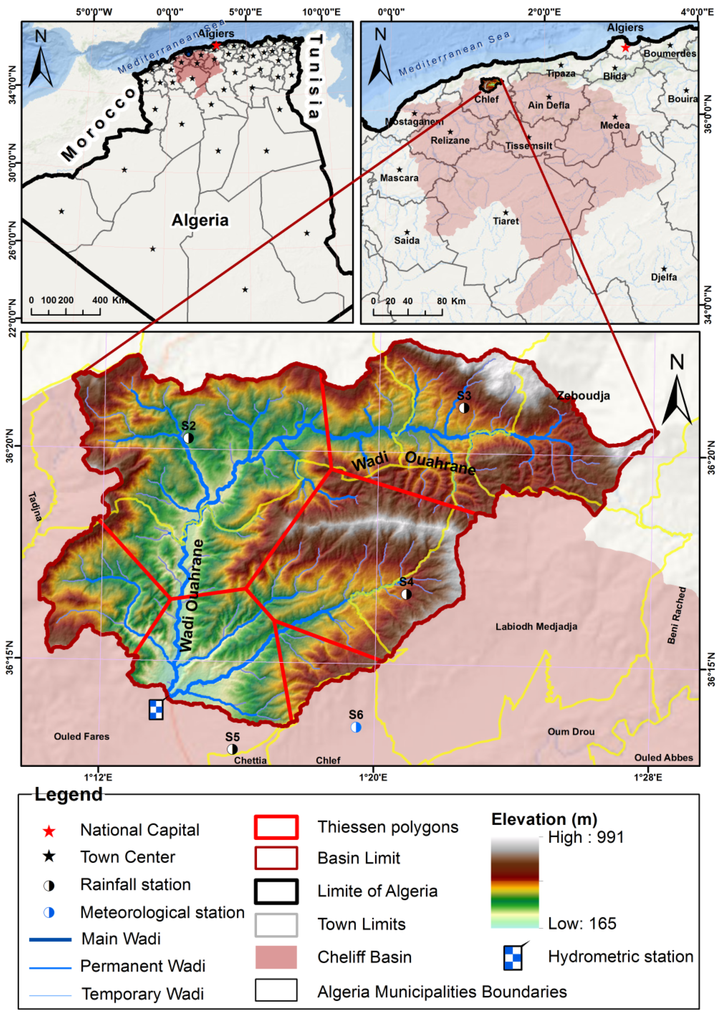
2. Study Area and Data Collection
3. Materials and Methods
3.1. SPI and SRI
3.2. Machine Learning Techniques
3.2.1. Artificial Neural Network
3.2.2. Adaptive Neuro-Fuzzy Inference System
3.2.3. Decision Trees
- All response variables and covariates are subjected to a global test of independence. If the outcome is not rejected, the procedure must be halted. Otherwise, the procedure proceeds to find the covariate that has the greatest impact on the response variable.
- In the adopted covariate, a binary split is performed.
3.2.4. Support Vector Machine
3.3. Performance Evaluation Criteria
4. Results and Discussion
5. Conclusions
Author Contributions
Funding
Institutional Review Board Statement
Informed Consent Statement
Data Availability Statement
Acknowledgments
Conflicts of Interest
References
- Williams, A.P.; Cook, E.R.; Smerdon, J.E.; Cook, B.I.; Abatzoglou, J.T.; Bolles, K.; Livneh, B. Large contribution from anthropogenic warming to an emerging North American megadrought. Science 2020, 368, 314–318. [Google Scholar] [CrossRef] [PubMed]
- Jiang, W.; Wang, L.; Zhang, M.; Yao, R.; Chen, X.; Gui, X.; Cao, Q. Analysis of drought events and their impacts on vegetation productivity based on the integrated surface drought index in the Hanjiang River Basin, China. Atmos. Res. 2021, 254, 105536. [Google Scholar] [CrossRef]
- Li, J.; Wang, Z.; Wu, X.; Zscheischler, J.; Guo, S.; Chen, X. A standardized index for assessing sub-monthly compound dry and hot conditions with application in China. Hydrol. Earth Syst. Sci. 2021, 25, 1587–1601. [Google Scholar] [CrossRef]
- Vicente-Serrano, S.M.; Van der Schrier, G.; Beguería, S.; Azorin-Molina, C.; Lopez-Moreno, J.I. Contribution of precipitation and reference evapotranspiration to drought indices under different climates. J. Hydrol. 2015, 526, 42–54. [Google Scholar] [CrossRef] [Green Version]
- Khan, N.; Sachindra, D.A.; Shahid, S.; Ahmed, K.; Shiru, M.S.; Nawaz, N. Prediction of droughts over Pakistan using machine learning algorithms. Adv. Water Resour. 2020, 139, 103562. [Google Scholar] [CrossRef]
- Heim, R.R., Jr. A review of twentieth-century drought indices used in the United States. Bull. Am. Meteorol. Soc. 2002, 83, 1149–1166. [Google Scholar] [CrossRef] [Green Version]
- Achite, M.; Wałęga, A.; Toubal, A.K.; Mansour, H.; Krakauer, N. Spatiotemporal characteristics and trends of meteorological droughts in the Wadi Mina Basin, Northwest Algeria. Water 2021, 13, 3103. [Google Scholar] [CrossRef]
- Habibi, B.; Meddi, M.; Torfs, P.J.; Remaoun, M.; Van Lanen, H.A. Characterisation and prediction of meteorological drought using stochastic models in the semi-arid Chéliff–Zahrez basin (Algeria). J. Hydrol. Reg. Stud. 2018, 16, 15–31. [Google Scholar] [CrossRef]
- Mishra, A.K.; Singh, V.P. Drought modeling–A review. J. Hydrol. 2011, 403, 157–175. [Google Scholar] [CrossRef]
- Jain, V.K.; Pandey, R.P.; Jain, M.K.; Byun, H.R. Comparison of drought indices for appraisal of drought characteristics in the Ken River Basin. Weather Clim. Extrem. 2015, 8, 1–11. [Google Scholar] [CrossRef] [Green Version]
- Kim, T.W.; Jehanzaib, M. Drought risk analysis, forecasting and assessment under climate change. Water 2020, 12, 1862. [Google Scholar] [CrossRef]
- Jehanzaib, M.; Bilal Idrees, M.; Kim, D.; Kim, T.W. Comprehensive evaluation of machine learning techniques for hydrological drought forecasting. J. Irrig. Drain. Eng. 2021, 147, 04021022. [Google Scholar] [CrossRef]
- Durbach, I.; Merven, B.; McCall, B. Expert elicitation of autocorrelated time series with application to e3 (energy-environment-economic) forecasting models. Environ. Model. Softw. 2017, 88, 93–105. [Google Scholar] [CrossRef]
- Bordi, I.; Sutera, A. Drought monitoring and forecasting at large scale. In Methods and Tools for Drought Analysis and Management; Springer: Dordrecht, The Netherlands, 2007; pp. 3–27. [Google Scholar]
- Soh, Y.W.; Koo, C.H.; Huang, Y.F.; Fung, K.F. Application of artificial intelligence models for the prediction of standardized precipitation evapotranspiration index (SPEI) at Langat River Basin, Malaysia. Comput. Electron. Agric. 2018, 144, 164–173. [Google Scholar] [CrossRef]
- Sari, Y.D.; Zarlis, M. Data-driven modelling for decision making under uncertainty. IOP Conf. Ser. Mater. Sci. Eng. 2018, 300, 012013. [Google Scholar]
- Adamowski, J.F. Development of a short-term river flood forecasting method for snowmelt driven floods based on wavelet and cross-wavelet analysis. J. Hydrol. 2008, 353, 247–266. [Google Scholar] [CrossRef]
- Sundararajan, K.; Garg, L.; Srinivasan, K.; Bashir, A.K.; Kaliappan, J.; Ganapathy, G.P.; Meena, T. A contemporary review on drought modeling using machine learning approaches. CMES-Comput. Model. Eng. Sci. 2021, 128, 447–487. [Google Scholar] [CrossRef]
- Yaseen, Z.M.; Ali, M.; Sharafati, A.; Al-Ansari, N.; Shahid, S. Forecasting standardized precipitation index using data intelligence models: Regional investigation of Bangladesh. Sci. Rep. 2021, 11, 1–25. [Google Scholar] [CrossRef] [PubMed]
- Dikshit, A.; Pradhan, B.; Alamri, A.M. Temporal hydrological drought index forecasting for New South Wales, Australia using machine learning approaches. Atmosphere 2020, 11, 585. [Google Scholar] [CrossRef]
- Feng, Y.; Cui, N.; Zhang, Q.; Zhao, L.; Gong, D. Comparison of artificial intelligence and empirical models for estimation of daily diffuse solar radiation in North China Plain. Int. J. Hydrog. Energy 2017, 42, 14418–14428. [Google Scholar] [CrossRef]
- Hassan, M.A.; Khalil, A.; Kaseb, S.; Kassem, M.A. Exploring the potential of tree-based ensemble methods in solar radiation modeling. Appl. Energy 2017, 203, 897–916. [Google Scholar] [CrossRef]
- Papadopoulos, S.; Azar, E.; Woon, W.L.; Kontokosta, C.E. Evaluation of tree-based ensemble learning algorithms for building energy performance estimation. J. Build. Perform. Simul. 2018, 11, 322–332. [Google Scholar] [CrossRef]
- Zhang, R.; Chen, Z.Y.; Xu, L.J.; Ou, C.Q. Meteorological drought forecasting based on a statistical model with machine learning techniques in Shaanxi province, China. Sci. Total Environ. 2019, 665, 338–346. [Google Scholar] [CrossRef]
- Li, J.; Wang, Z.; Wu, X.; Xu, C.Y.; Guo, S.; Chen, X.; Zhang, Z. Robust meteorological drought prediction using antecedent SST fluctuations and machine learning. Water Resour. Res. 2021, 57, e2020WR029413. [Google Scholar] [CrossRef]
- Mohamadi, S.; Sammen, S.S.; Panahi, F.; Ehteram, M.; Kisi, O.; Mosavi, A.; Al-Ansari, N. Zoning map for drought prediction using integrated machine learning models with a nomadic people optimization algorithm. Nat. Hazards 2020, 104, 537–579. [Google Scholar] [CrossRef]
- Nabipour, N.; Dehghani, M.; Mosavi, A.; Shamshirband, S. Short-term hydrological drought forecasting based on different nature-inspired optimization algorithms hybridized with artificial neural networks. IEEE Access 2020, 8, 15210–15222. [Google Scholar] [CrossRef]
- Shen, R.; Huang, A.; Li, B.; Guo, J. Construction of a drought monitoring model using deep learning based on multi-source remote sensing data. Int. J. Appl. Earth Obs. Geoinf. 2019, 79, 48–57. [Google Scholar] [CrossRef]
- Adikari, K.E.; Shrestha, S.; Ratnayake, D.T.; Budhathoki, A.; Mohanasundaram, S.; Dailey, M.N. Evaluation of artificial intelligence models for flood and drought forecasting in arid and tropical regions. Environ. Model. Softw. 2021, 144, 105136. [Google Scholar] [CrossRef]
- Mokhtar, A.; Jalali, M.; He, H.; Al-Ansari, N.; Elbeltagi, A.; Alsafadi, K.; Rodrigo-Comino, J. Estimation of SPEI meteorological drought using machine learning algorithms. IEEE Access 2021, 9, 65503–65523. [Google Scholar] [CrossRef]
- Future Directions International Pty Ltd. Water Protests in Algeria Are Giving Cause for Concern about Its Long-Term Stability. Available online: https://www.futuredirections.org.au/publication/water-protests-in-algeria-are-giving-cause-for-concern-about-its-long-term-stability/ (accessed on 6 December 2021).
- Awange, J.L.; Mpelasoka, F.; Goncalves, R.M. When every drop counts: Analysis of droughts in Brazil for the 1901-2013 period. Sci. Total Environ. 2016, 566, 1472–1488. [Google Scholar] [CrossRef] [Green Version]
- Naresh Kumar, M.; Murthy, C.S.; Sesha Sai, M.V.R.; Roy, P.S. On the use of Standardized Precipitation Index (SPI) for drought intensity assessment. Meteorol. Appl. 2009, 16, 381–389. [Google Scholar] [CrossRef] [Green Version]
- McKee, T.B.; Doesken, N.J.; Kliest, J. The Relationship of Drought Frequency and Duration to Time Scales. In Proceedings of the 8th Conference on Applied Climatology, Anaheim, CA, USA, 17–22 January 1993. [Google Scholar]
- See, L.; Openshaw, S. Applying soft computing approaches to river level forecasting. Hydrol. Sci. J. 1999, 44, 763–778. [Google Scholar] [CrossRef] [Green Version]
- Mishra, A.K.; Desai, V.R. Drought forecasting using stochastic models. Stoch. Environ. Res. Risk Assess. 2005, 19, 326–339. [Google Scholar] [CrossRef]
- Jang, J.S.R.; Sun, C.T.; Mizutani, E. Neuro-fuzzy and soft computing-a computational approach to learning and machine intelligence [Book Review]. IEEE Trans. Automat. Contr. 1997, 42, 1482–1484. [Google Scholar] [CrossRef]
- Gholami, A.; Bonakdari, H.; Zaji, A.H.; Ajeel Fenjan, S.; Akhtari, A.A. Design of modified structure multi-layer perceptron networks based on decision trees for the prediction of flow parameters in 90 open-channel bends. Eng. Appl. Comput. Fluid Mech. 2016, 10, 193–208. [Google Scholar] [CrossRef] [Green Version]
- Mokhtarzad, M.; Eskandari, F.; Vanjani, N.J.; Arabasadi, A. Drought forecasting by ANN, ANFIS, and SVM and comparison of the models. Environ. Earth Sci. 2017, 76, 1–10. [Google Scholar] [CrossRef]
- Alipour, Z.; Ali, A.M.A.; Radmanesh, F.; Joorabyan, M. Comparison of three methods of ANN, ANFIS and time series models to predict ground water level:(Case study: North Mahyar plain). BEPLS 2014, 3, 128–134. [Google Scholar]
- Breiman, L.; Friedman, J.; Olshen, R.; Stone, C. Classification and Regression Trees; CRC Press: Boca Raton, FL, USA, 1984. [Google Scholar]
- McClean, S.I. Data mining and knowledge discovery. In Encyclopedia of Physical Science and Technology; Academic Press: Cambridge, MA, USA, 2003; pp. 229–246. [Google Scholar]
- Vapnik, V. The Nature of Statistical Learning Theory, 2nd ed.; Springer Science & Business Media: New York, NY, USA, 1999. [Google Scholar]
- Belayneh, A.; Adamowski, J.; Khalil, B.; Ozga-Zielinski, B. Long-term SPI drought forecasting in the Awash river basin in Ethiopia using wavelet neural network and wavelet support vector regression models. J. Hydrol. 2014, 508, 418–429. [Google Scholar] [CrossRef]
- Deka, P.C. Support vector machine applications in the field of hydrology: A review. Appl. Soft Comput. 2014, 19, 372–386. [Google Scholar]
- Belayneh, A.; Adamowski, J. Drought forecasting using new machine learning methods. J. Water Land Dev. 2013, 18, 3–12. [Google Scholar] [CrossRef]
- Elshaboury, N.; Marzouk, M. Comparing Machine Learning Models for Predicting Water Pipelines Condition. In Proceedings of the 2020 2nd Novel Intelligent and Leading Emerging Sciences Conference (NILES), Giza, Egypt, 24–26 October 2020; pp. 134–139. [Google Scholar]
- Abdelkader, E.M.; Al-Sakkaf, A.; Elshaboury, N.; Alfalah, G. On the Implementation of Machine Learning Models for Emulating Daily Electricity Consumption in Hotel Facilities. In Proceedings of the 6th World Congress on Civil, Structural, and Environmental Engineering (CSEE’21), Lisbon, Portugal, 21–23 June 2021. [Google Scholar]
- Elshaboury, N. Assessment of Different Artificial Neural Networks for Predicting Bridge Deck Condition. In Proceedings of the 4th Smart Cities Symposium (SCS21), Zallaq, Bahrain, 21–23 November 2021. [Google Scholar]
- Idrees, M.B.; Jehanzaib, M.; Kim, D.; Kim, T.W. Comprehensive evaluation of machine learning models for suspended sediment load inflow prediction in a reservoir. Stoch. Environ. Res. Risk Assess. 2021, 35, 1805–1823. [Google Scholar] [CrossRef]


| Stations | ID | Name | Geographical Coordinates (° ′ ″) | Elevation (m) | |
|---|---|---|---|---|---|
| Longitude | Latitude | ||||
| Rainfall stations | |||||
| S1 | 012201 | LARBAT OULED FARES | 01°09′18″ | 36°16′20″ | 116 |
| S2 | 012224 | BOUZGHAIA | 01°14′27″ | 36°20′15″ | 217 |
| S3 | 012205 | BENAIRIA | 01°22′28″ | 36°21′04″ | 320 |
| S4 | 012221 | MEDJAJA | 01°20′53″ | 36°16′39″ | 487 |
| S5 | 012209 | CHETIA | 01°15′53″ | 36°12′56″ | 108 |
| S6 | NMO | Airport, Chlef | 01°19′28″ | 36°13′31″ | 158 |
| Hydrometric station | |||||
| S1 | 012201 | LARBAT OULED FARES | 01°13′5″ | 36°14′14″ | 173 |
| State | SPI/SRI Range | |
|---|---|---|
| Minimum | Maximum | |
| Extremely wet | ≥2.0 | |
| Severely wet | 1.50 | 1.99 |
| Moderately wet | 1.00 | 1.49 |
| Near normal | −0.99 | 0.99 |
| Moderately dry | −1.49 | −1.00 |
| Severely dry | −1.99 | −1.50 |
| Extremely dry | ≤−2.0 | |
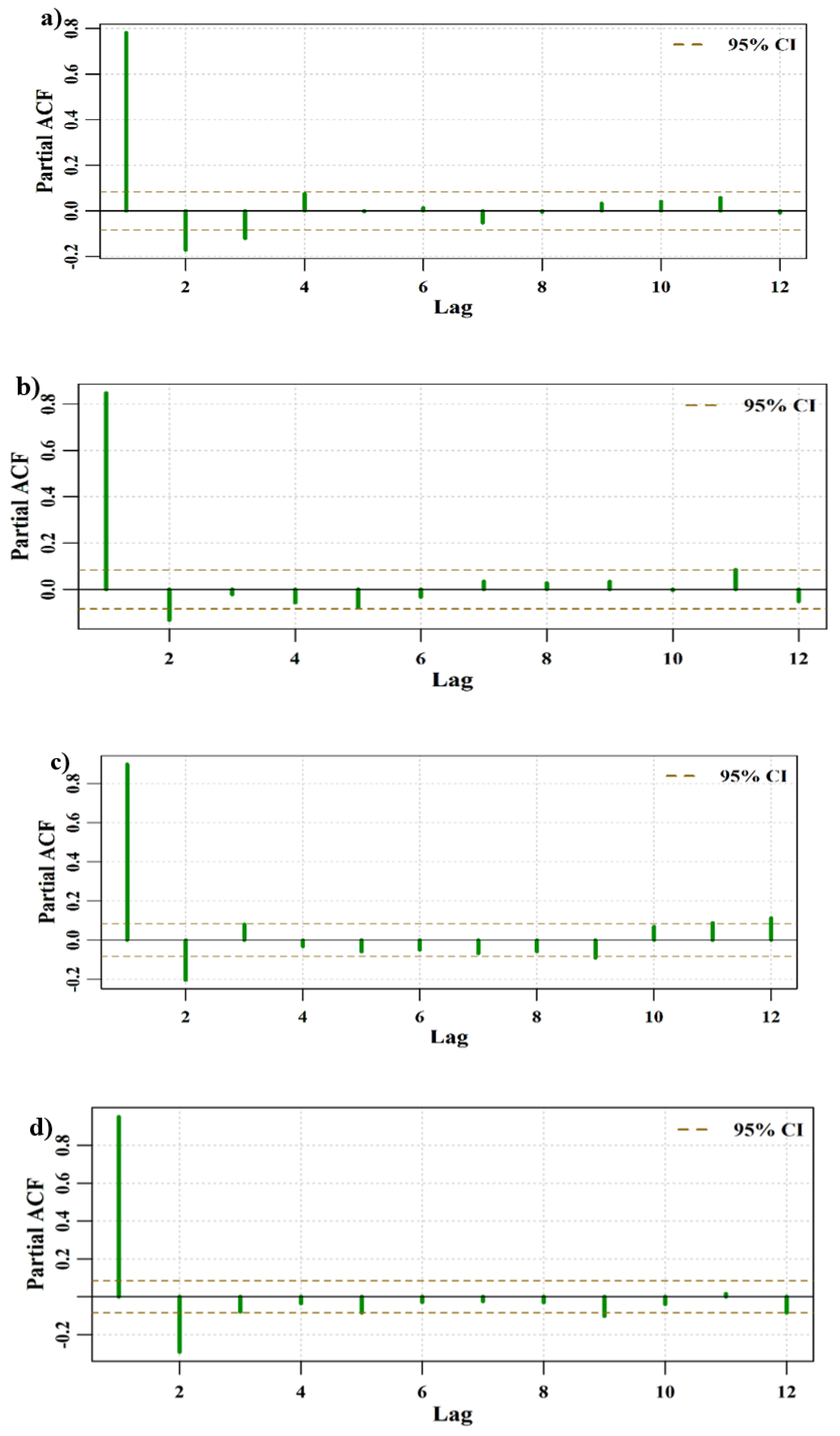
| Station Name | Input Variables | Target Variable |
|---|---|---|
| LARBAT OULED FARES | SPI-5, SRI-3(t−1), SRI-3(t−2), SRI-3(t−3) | SRI-3 |
| SPI-6, SRI-6(t−1), SRI-6(t−2), SRI-6(t−11) | SRI-6 | |
| SPI-10, SRI-9(t−1), SRI-9(t−2), SRI-9(t−9), SRI-9(t−11), SRI-9(t−12) | SRI-9 | |
| SPI-12, SRI-12(t−1), SRI-12(t−2), SRI-12(t−9) | SRI-12 |
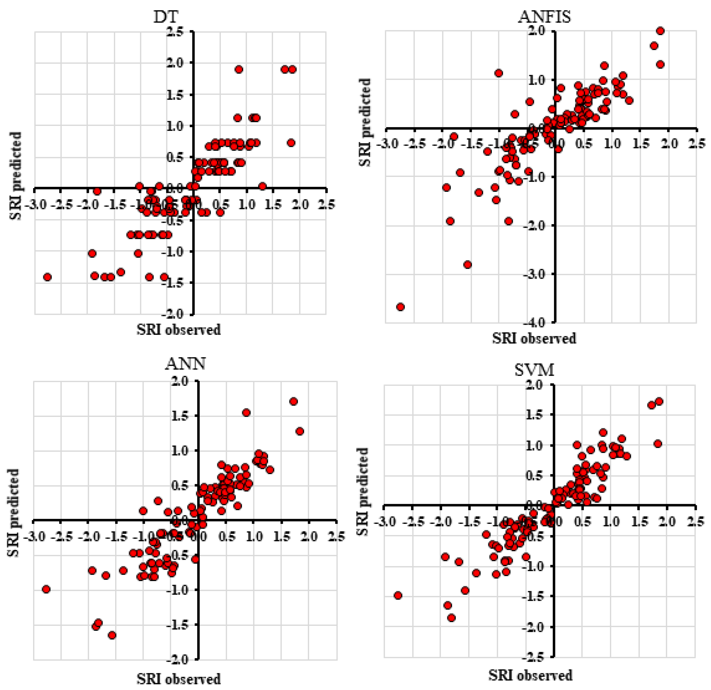
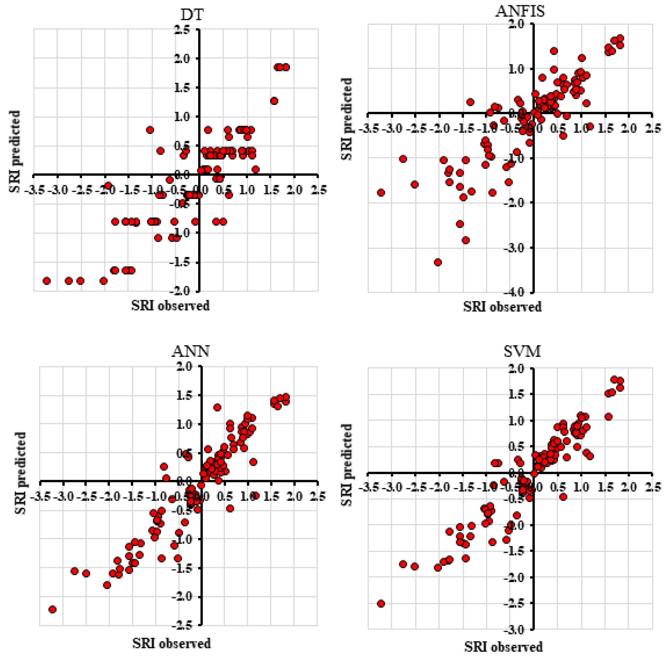
| ML Model | Timescale | Performance Indicators | |||
|---|---|---|---|---|---|
| RMSE | MAE | NSE | R2 | ||
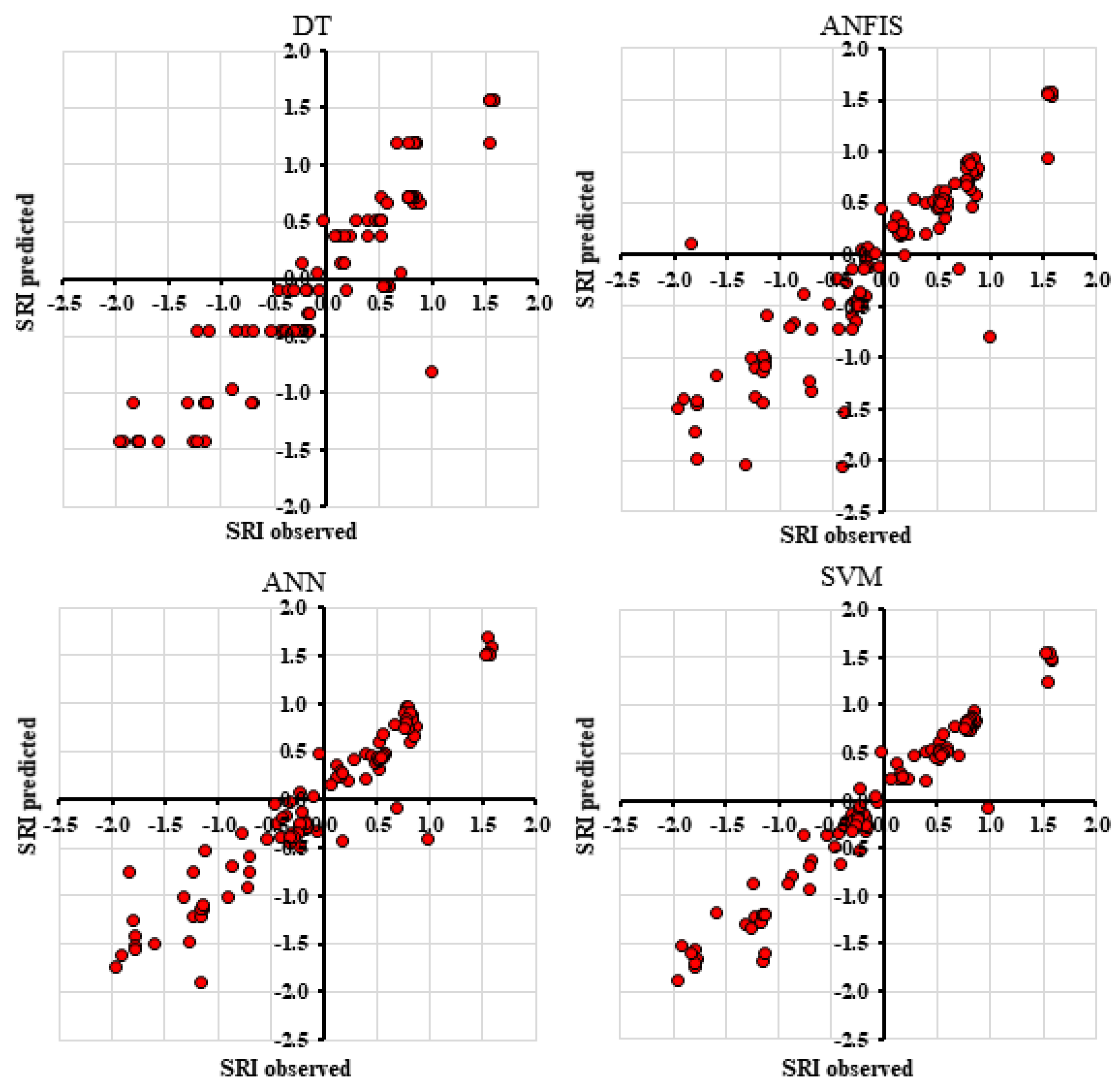
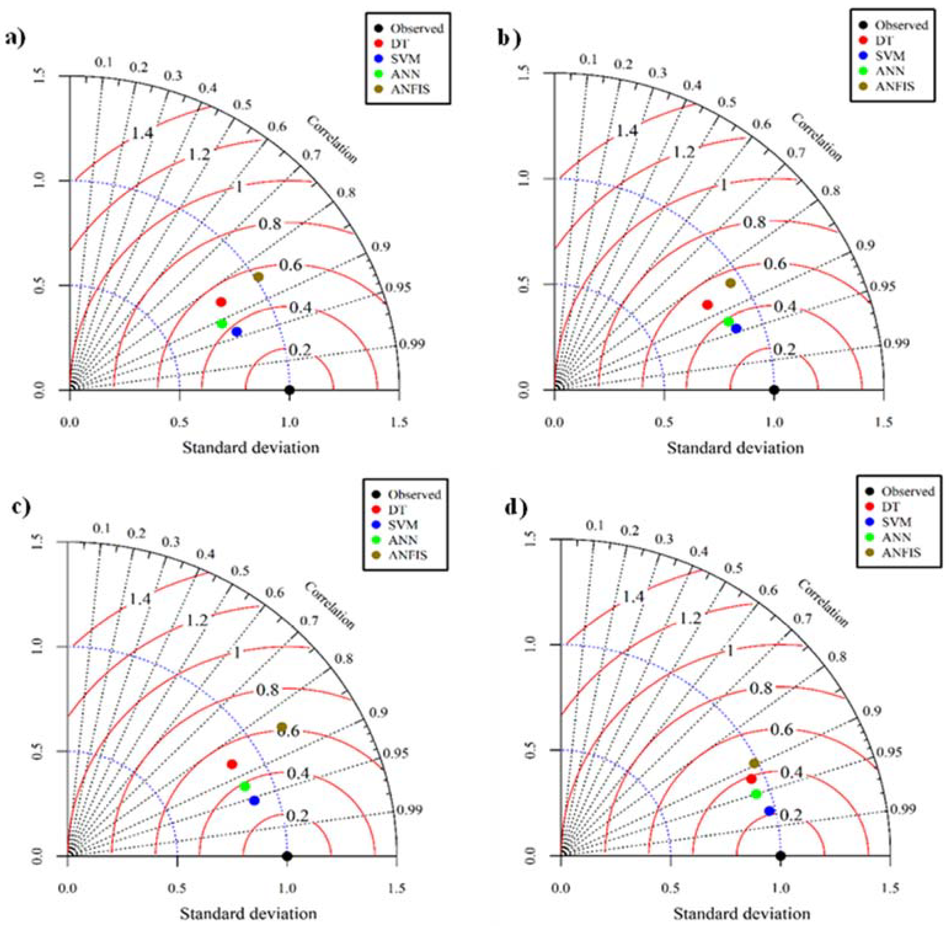
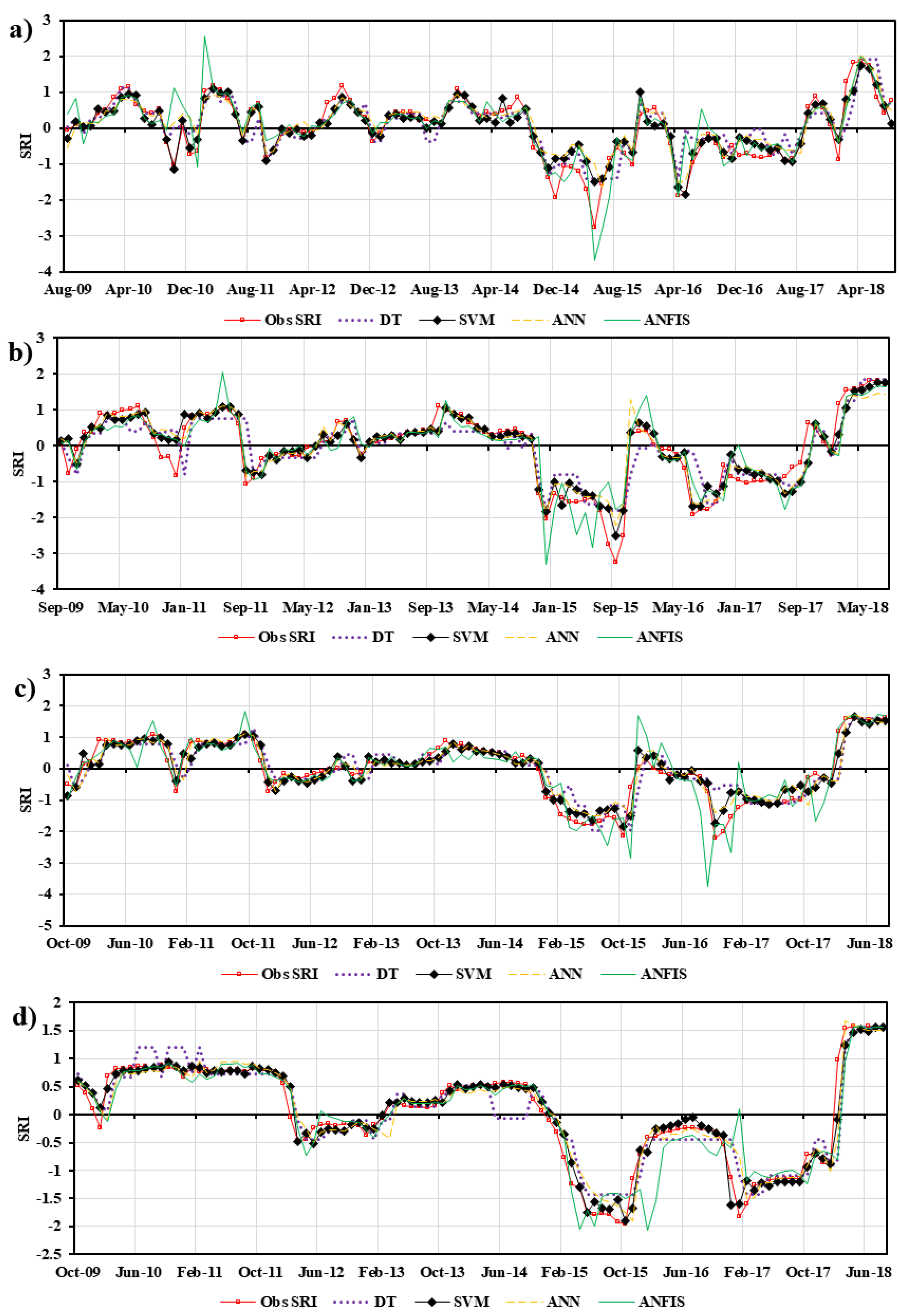
| DT | 3 months | 0.45 | 0.31 | 0.57 | 0.73 |
| 6 months | 0.51 | 0.35 | 0.61 | 0.75 | |
| 9 months | 0.46 | 0.31 | 0.66 | 0.74 | |
| 12 months | 0.34 | 0.23 | 0.83 | 0.85 | |
| ANFIS | 3 months | 0.48 | 0.32 | 0.69 | 0.72 |
| 6 months | 0.55 | 0.39 | 0.67 | 0.72 | |
| 9 months | 0.57 | 0.33 | 0.71 | 0.71 | |
| 12 months | 0.4 | 0.23 | 0.79 | 0.8 | |
| ANN | 3 months | 0.39 | 0.27 | 0.64 | 0.83 |
| 6 months | 0.37 | 0.26 | 0.8 | 0.86 | |
| 9 months | 0.35 | 0.24 | 0.8 | 0.86 | |
| 12 months | 0.27 | 0.17 | 0.89 | 0.9 | |
| SVM | 3 months | 0.31 | 0.22 | 0.79 | 0.88 |
| 6 months | 0.34 | 0.24 | 0.85 | 0.89 | |
| 9 months | 0.28 | 0.2 | 0.88 | 0.91 | |
| 12 months | 0.19 | 0.12 | 0.95 | 0.95 | |
| Sr. No. | ML Models | Average Computation Time (s) |
|---|---|---|
| 1 | ANN | 11.65 |
| 2 | ANFIS | 28.35 |
| 3 | DT | 1.37 |
| 4 | SVM | 0.15 |
Publisher’s Note: MDPI stays neutral with regard to jurisdictional claims in published maps and institutional affiliations. |
© 2022 by the authors. Licensee MDPI, Basel, Switzerland. This article is an open access article distributed under the terms and conditions of the Creative Commons Attribution (CC BY) license (https://creativecommons.org/licenses/by/4.0/).
Share and Cite
Achite, M.; Jehanzaib, M.; Elshaboury, N.; Kim, T.-W. Evaluation of Machine Learning Techniques for Hydrological Drought Modeling: A Case Study of the Wadi Ouahrane Basin in Algeria. Water 2022, 14, 431. https://doi.org/10.3390/w14030431
Achite M, Jehanzaib M, Elshaboury N, Kim T-W. Evaluation of Machine Learning Techniques for Hydrological Drought Modeling: A Case Study of the Wadi Ouahrane Basin in Algeria. Water. 2022; 14(3):431. https://doi.org/10.3390/w14030431
Chicago/Turabian StyleAchite, Mohammed, Muhammad Jehanzaib, Nehal Elshaboury, and Tae-Woong Kim. 2022. "Evaluation of Machine Learning Techniques for Hydrological Drought Modeling: A Case Study of the Wadi Ouahrane Basin in Algeria" Water 14, no. 3: 431. https://doi.org/10.3390/w14030431