A Model-Based Approach for Improving Surface Water Quality Management in Aquaculture Using MIKE 11: A Case of the Long Xuyen Quadangle, Mekong Delta, Vietnam

Abstract

This study utilized MIKE 11 to quantify the spatio-temporal dynamics of water quality parameters (Biochemical Oxygen Demand (BOD₅), Dissolved Oxygen (DO) and temperature) in the Long Xuyen Quadrangle area of the Vietnamese Mekong Delta. Calibrated for the year of 2019 and validated for the year of 2020, the developed model showed a significant agreement between the observed and simulated values of water quality parameters. Locations near to cage culture areas exhibited higher BOD₅ values than sites close to pond/lagoon culture areas due to the effects of numerous point sources of pollution, including upstream wastewater and out-fluxes from residential and tourism activities in the surrounding areas, all of which had a direct impact on the quality of the surface water used for aquaculture. Moreover, as aquacultural effluents have intensified and dispersed over time, water quality in the surrounding water bodies has degraded. The findings suggest that the effective planning, assessment and management of rapidly expanding aquaculture sites should be improved, including more rigorous water quality monitoring, to ensure the long-term sustainable expansion and development of the aquacultural sector in the Long Xuyen Quadrangle in particular, and the Vietnamese Mekong Delta as a whole.

1. Introduction

Globally, demand for freshwater resources continues to increase. Freshwater sources are increasingly required to meet growing domestic, agriculture, aquaculture and industrial uses, while at the same time they suffer from increased pollution and natural and anthropogenic interventions and changes to the environment driven by strong population and economic growth [1,2,3,4]. In Southeast Asia, poorly managed aquacultural and agricultural activities are one of the most prominent sources of water pollution [2,5,6,7,8,9]. Here, countries find it challenging to manage surface water quality due to both point and non-point sources of pollutants, as well as the increased widespread use of chemicals and drugs in the context of limited land and water resources and more intensive culture methods [10,11,12]. Due of the cumulative and synergistic impacts on water resources, water quality management requires a fundamental understanding of the spatial and temporal variations in water characteristics, including the hydro-morphological, chemical and biological parameters [13]. Previously, several methods have been developed to predict, monitor and assess water quality. These include using hydrogeochemical analysis [14,15,16,17], the use of various quality indexes [2,18,19], using numerical modeling for scenario development [20,21] and using socio-hydrological approaches to assess the nexus between water and human well-being [22]. All these approaches seek to provide a better understanding of the drivers and interlinkages at work, and to help decision makers take evidence-based actions with regard to improved water resource management.

However, using traditional hydro-chemical analysis and statistical approaches for analyzing the dynamics of water quality have inherent limitations when considering the different environmental components in a holistic manner. Moreover, they tend to be resource (money and human power) intensive. As a result, numerical simulation models or tools, including environmental modeling, that are capable of detecting regional and temporal changes in current and future water quality or quantity parameters are currently gaining increased popularity among scientists and water management practitioners [23,24]. In addition, the application of numerical simulations can also save labor, time and money [24,25].

Various hydraulics models, such as the Hydrological Engineering Centre—River Analysis System (HEC-RAS), MIKE 11 and Vietnamese River System and Plain (VRSAP) have been previously applied in the VMD to assess the changes in the quantity and quality of water in rivers, as well as quantify the impact of land management practices on water quality [26,27,28]. These models are holistic in nature and attempt to take into account the all-important environmental processes [16,20,21]. Because of its robust nature, the MIKE 11 model has previously been extensively used to investigate water security issues, especially in Asia [29].

As a rapidly developing and lower riparian country, Vietnam is particularly susceptible to water resource changes [30,31]. Southeast Asia’s longest river, the Mekong River, appears to have its source on the Tibetan plateau, and runs through China, Myanmar, Laos, Thailand and Cambodia before reaching Vietnam. At its end, the Vietnamese Mekong Delta (VMD) is one of the world’s largest river deltas, with a dense network of rivers, canals and ditches, and covering over 4 million hectares, which is approximately 12 percent of Vietnam’s natural land area [32]. The VMD is also the largest agricultural and aquacultural hub in Vietnam, accounting for 50% of rice, 65% of aquaculture and 70% of fruit production, as well as including 95% of exported rice and 60% of exported fish [33].

The Long Xuyen Quadrangle (LXQ), as shown in Figure 1, is the first area in Vietnam to collect and use water from the Mekong River via two main branches, the Bassac River and the Mekong River. However, in the last few decades, water pollution has been an increasing problem in the delta [1,2,8,34]. The principal sources of pollution are non-point sources, such as wastewater discharged without treatment from industrial zones and commercial activities along the banks of rivers or canals. Furthermore, within the LXQ, intensive freshwater farming activities in the provinces of An Giang, Kien Giang and Can Tho city affect directly the water quality. In spite of its high regional importance and socio-economic significance, very few studies have investigated the water resources of LXQ in an in-depth, comprehensive and holistic manner.

Against this background, our study aims to apply a hydrological simulation to investigate the spatio-temporal dynamics of key water quality parameters using MIKE 11. The hydrodynamic module, the structural operation module, the advection/dispersion module and the EcoLab module are all inclusive of the MIKE 11 model system. The outcomes of this study will firstly help decision makers to understand the current situation, and secondly help the design of future management options for improved water resource management.

2. Materials and Methods

The LXQ covers a large portion of the An Giang and Kien Giang provinces, and a small portion of Can Tho city, with a total area of approximately 0.5 million hectares. It is bordered to the north by the Bassac River and the Vietnamese–Cambodian border, to the south by the Cai San Canal, and to the west by the West Sea of Vietnam (Gulf of Thailand) [23]. Like the VMD as a whole, the topography of the LXQ, is relatively low and flat, with ground elevations of 0–1.0 m above mean sea level accounting for over 80% of the area [35,36]. The tropical monsoon climate of LXQ, has two primary seasons, dry and wet, and it is hot and humid all year round. As a result, LXQ’s average annual temperature, rainfall and humidity are approximately 27°C, 1200 mm and 80%, respectively [36].

The LXQ is significantly affected by its geographical location, its monsoon climate and the upstream river network and the tidal regime [35,37]. Within the LXQ, the yearly average flow of the river systems is around 14,000 m³·s⁻¹. However, this can reach up to 24,000 m³·s⁻¹ during the rainy season, and recede to only 5000 m³·s⁻¹ during the dry season [36]. During the rainy season, annual floods inundate roughly 70% of the total LXQ area with water levels of 1.0–2.5 m for 3–5 months a year. This episodic flooding has both positive and negative effects to the socio-economic signature of this region. On the positive side, floodwaters bring large volumes of water for agriculture, aquaculture, domestic uses and industrial operations, and provide the region with nutrient-rich sediments, as well as helping to wash out pollutants and salinity from the soil. Flood disasters, on the other hand, severely damage infrastructure, interrupt both community and livelihood activities and jeopardize agricultural and fishery production [38,39]. As a result, both the provincial and national governments have made significant investments in local infrastructure to regulate water levels and protect the region through a series of full-dyke and semi-dyke systems [36]. However, this has resulted in changes to the hydrometeorological regime and fluxes, and lessened the potential for water pollutant dispersion.

To simulate water quality in the complex and dense river network of LXQ, this study utilized the hydrodynamics and EcoLab modules, which are the foundation of the one-dimensional (1-D) MIKE 11 model.

Various hydro-meteorological data used as input for the modeling were kindly provided from a variety of sources, including the Southern Institute of Water Resources Research (SIWRR), the Southern Region Hydro-Meteorological Centre (SRHMC), the Department of Natural Resources and Environment (DoNRE), and the Department of Agriculture and Rural Development (DARD) (

Table 1. Summary of hydrology and water quality data collection and sources.

Data	Sources	Period	Remarks
Water level	The Southern Region Hydro-Meteorological Centre (SRHMC)	Jan.–May, 2019 Jan.–May, 2020	Time-step: Hourly data
Discharge	The Southern Region Hydro-Meteorological Centre (SRHMC)	Jan.–May, 2019 Jan.–May, 2020	Time-step: Hourly data
Cross-section	GIZ	-	-
DO, Temperature, BOD5	DoNRE, DARD	Jan.–May, 2019 Jan.–May, 2020	Time-step: Monthly data

). Additional data regarding the population, wastewater discharge, pollution load of BOD₅ and the current land use map were collected from residential, industrial, aquacultural and agricultural areas to estimate the pollution load discharges.

Within the study area, hourly observations of the discharge were conducted at two stations at Chau Doc and Vam Nao, and these were used as the upstream boundary conditions, and hourly observations of the water level were conducted at two stations at Rach Gia and Can Tho, and these were used as the downstream boundary conditions. The hourly discharge and water level at Long Xuyen were obtained for calibration and verification for the years 2019 and 2020 for the period from 00:00 a.m. on 1st January to 23:59 p.m. on 31st May. Average monthly water quality data, such as BOD₅, DO and temperature, were also obtained at eight stations from January to May in 2019 and 2020 for calibration and validation, respectively.

The total estimated fishery production for the year 2019 was 532.6 thousand tons, with pangasius production accounting for 412 tons in the study area. In 2020, due to the impact of the COVID-19 pandemic, the export of pangasius encountered many difficulties with the selling price becoming low, so farmers and businesses cut back on feed to prolong farming time, waiting for the price to increase, leading to a decrease in the harvest, with 211 thousand tons produced from the month of January to May 2020 [40]. Fish are mostly cultured in ponds and lagoons on both banks of the Bassac River, as well as along the tributaries Bay Tre, Xa Doi Canal, Cai Sao Canal, Don Dong Canal and Moi Canal (Figure 1 and

Table A1. Location of aquaculture ponds and lagoons in the study area.

Location of Ponds and Lagoons	Locations of Water Quality Monitoring
Ponds and lagoons in Vinh Thanh Trung (Vinh Tre Canal)	TS5(TĐ)-CP
Ponds and lagoons Binh Thanh (Hau River)	TS6(TĐ)-CT
Ponds and lagoons My Hoa Hung (Hau River)	TS7(TĐ)-LX
Ponds and lagoons My Hoa Hung	TS8(TĐ)-LX
Ponds and lagoons Phu Thuan (Xa Doi Canal)	TS10(TĐ)-TS
Ponds and lagoons My Thoi (Cai Sao River)	TS11(TĐ)-LX
Ponds and lagoons Phú Thuận (Don Dong Canal)	TS12(TĐ)-TS
Ponds and lagoons Vinh Hanh (Nui Chac Canal)	TS13(TĐ)-CT
Ponds and lagoons Phu Thuan (Don Dong Canal)	TS14(TĐ)-TS
Ponds and lagoons Vinh Khanh (Cai Sao River)	TS15(TĐ)-TS

).

2.1. Estimation of Pollution Load

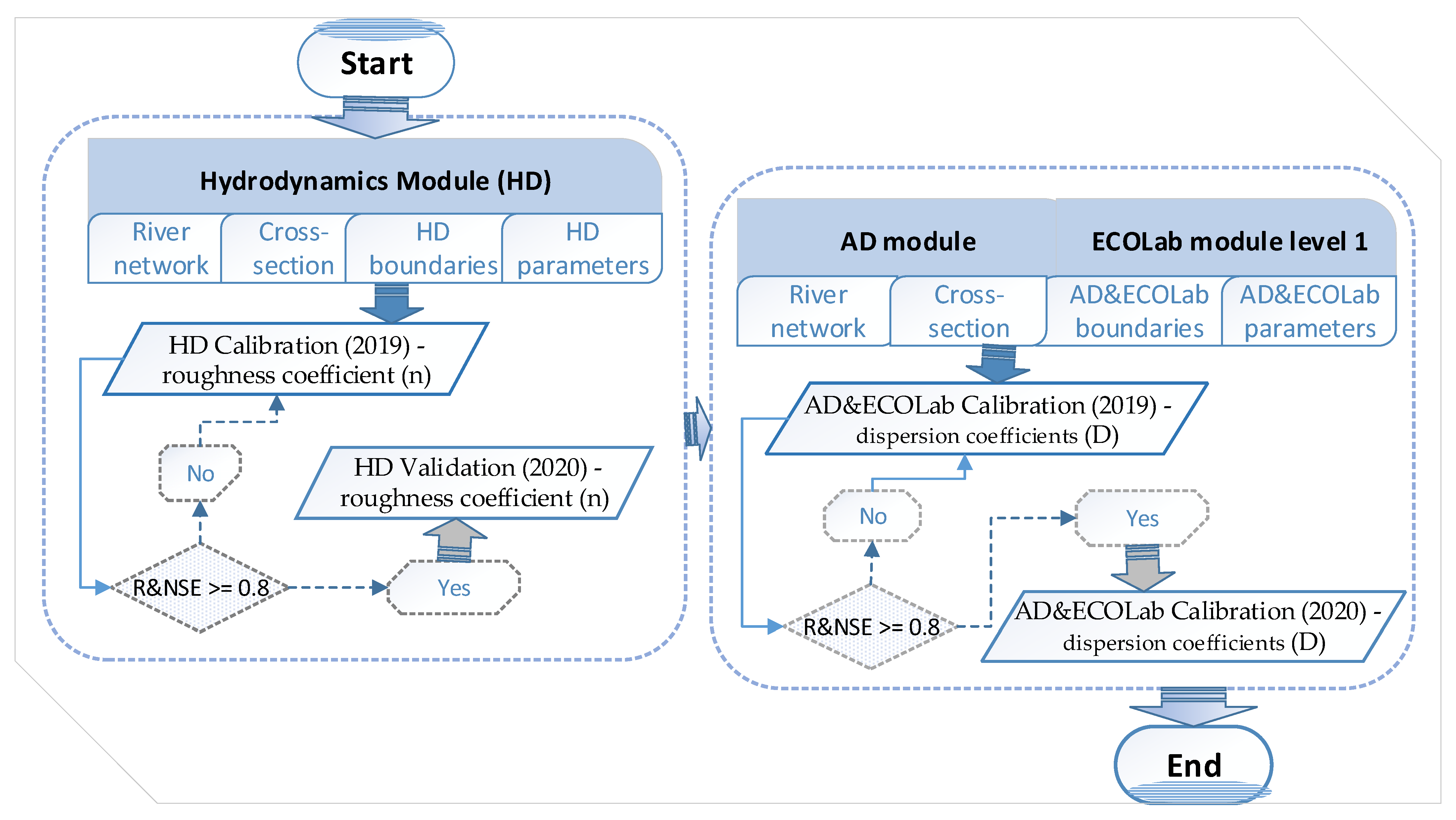
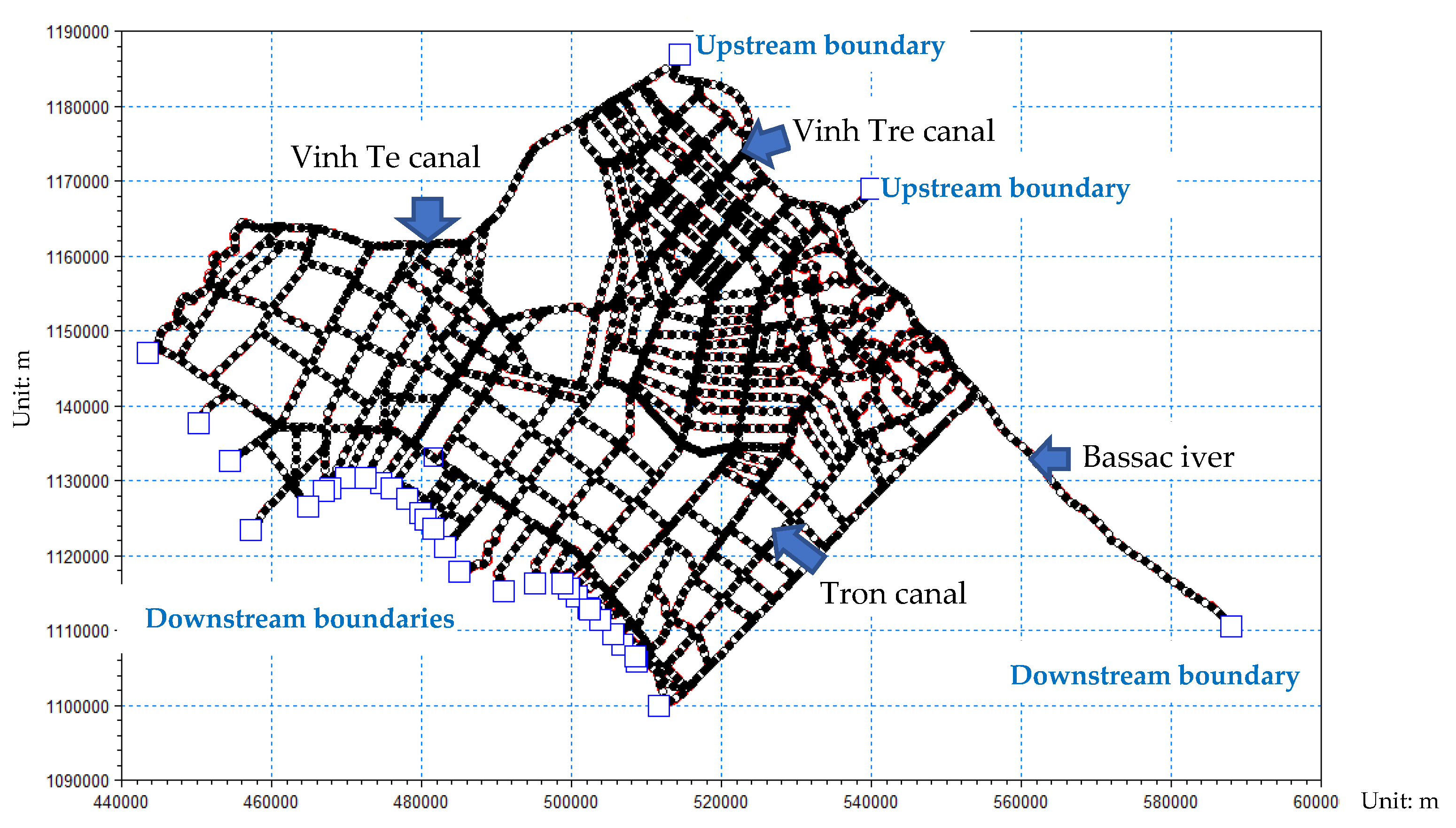
Previous studies have estimated pollution load in various Vietnamese river networks, and found the ratio of BOD₅/Chemical Oxygen Demand (COD) to be around 0.65 [41,42]. This suggests that the majority of organic pollutants are soluble and easily decomposable. However, because of a lack of observed data in the study area, the pollutant load was calculated using the BOD₅ concentration as an indicator. Pollution load was computed using the discharge estimate, using Equation (1) as shown below:

$${\mathrm{Q}}_{\mathrm{M}}{=\mathrm{Q}\times \mathrm{C}}_{\mathrm{i}}$$

(1)

where Q_M denotes the pollution load from the Mekong River (tons·year⁻¹), Q denotes the discharge (m³·s⁻¹) and C_i is the concentration of parameter i (mg·L⁻¹).

For domestic sources, pollution load was calculated based on the population statistics in the study area. The pollution emission coefficient per capita was calculated using Equation (2), as shown below:

$${\mathrm{Q}}_{\mathrm{D}}{=\mathrm{P} \times \mathrm{Q}}_{\mathrm{i}}$$

(2)

where Q_D is pollution load from the population (tons·year⁻¹), P is the population of the area (persons) and Q_i is the domestic waste load of parameter i (kg·person⁻¹·year⁻¹) (

Table 2. Pollution load estimation.

Pollution Load	BOD5 (mg·L−1)
Domestic waste load (kg/person/year)	10–25
Poultry (kg/unit/year)	2.73
Cow, buffalo (kg/unit/year)	233.6
Pig (kg/unit/year)	73
Sutchi catfish farming (kg/unit/year)	8.1

).

For industrial areas, the pollution load was estimated by multiplying the industrial discharge (Q) by the pollutant emission coefficient of the industrial type, using Equation (3) as shown below:

$${\mathrm{Q}}_{\mathrm{I}}={\displaystyle \sum }_{\mathrm{j}=1}^{\mathrm{n}}{\mathrm{V}}_{\mathrm{j}}{ \times \mathrm{C}}_{\mathrm{i},\mathrm{j}}$$

(3)

where Q_I is the pollution load from industries, V_j is the volume of annual wastewater discharged from industry j (m³·year⁻¹), C_i,j is the concentration of substance i in the wastewater of industry j (mg·L⁻¹) and n is the number of industries in the region.

The pollution load from livestock production activities was calculated using the total annual livestock herd and the unit of discharge load for livestock and poultry, using Equation (4) as shown below:

$${\mathrm{Q}}_{\mathrm{L}}{=\mathrm{n} \times \mathrm{Q}}_{\mathrm{i}}$$

(4)

where Q_L is the pollution load from livestock (tons·year⁻¹), n is the number of livestock and poultry (unit) and Q_i is the load of parameter i (kg·unit⁻¹·year⁻¹).

The pollution load arising from aquaculture sources was calculated based on the aquacultural area and the coefficient of each waste generation for each different form of aquaculture, using Equation (5) as shown below:

$${\mathrm{Q}}_{\mathrm{A}}{=\mathrm{Q}}_{\mathrm{i}} \times \mathrm{S} \times \mathrm{t}$$

(5)

where Q_A is the pollution load from aquacultural activities (tons·year⁻¹), Q_i is the load of the pollution source (kg·ha⁻¹·day⁻¹), S is the area of land used for farming (ha), and t is the time of farming in the year (day).

Table 2 shows the calculation of the waste load generated on the basis of system emissions according to UNEP (1984) [43], San Diego-McGlone (2000) [41]. This estimation method has been successfully applied to many studies [44,45].

2.2. Model Setup

MIKE is a suite of software applications developed by the Danish Hydraulic Institute (DHI), consisting of different models (MIKE 11, MIKE 21, MIKE 3, MIKE SHE, Mouse and MIKE Basin), to accurately analyze, model and simulate rivers, lakes, estuaries and coastal environments. MIKE 11 includes the hydrodynamic module (HD) and EcoLab. The HD module permits the simulation of water levels, discharge and the discharge of wastewaters, while the EcoLab module (WQ module) describes how pollutants travel and disperse along rivers or channels over time. The HD module, applied on open-channel flows, solves finite differences from Saint-Venant equations consisting of the mass conservation and fluid momentum conservation, based on the following assumptions: (i) the flow is a dimension, with depth and velocity varying in the longitudinal direction of the channel; (ii) the bottom slope is small, and scour and deposition are negligible and the channel bed is fixed; (iii) flow everywhere is parallel to the bottom (i.e., wavelengths are large compared with water depths); (iv) the flow is sub-critical; (v) the water is incompressible and homogeneous, i.e., without significant variation in density; and (vi) the lateral inflow does not affect velocity in the channel.

The EcoLab module is based on the conservation of mass, which is a basic principle of the water quality model. It involves performing a mass balance for a defined control volume over a specified period of time. The EcoLab module is coupled to the AD module; while the EcoLab module deals with the transforming processes of compounds in the river, the AD module is used to simulate the simultaneous transport process. The AD equation is based on the following main assumptions: (i) the considered substance is completely mixed over the cross-section, (ii) the substance is conservative or subject to a first-order reaction (linear decay); and (iii) Fick’s diffusion law is applied. Fick’s law assumes that the mass flux is proportional to the gradient of the mean concentration and that the flux is in the direction of decreasing concentration. Dependent on the nature of the water quality problem under consideration, the model can be adjusted to different levels of detail. The complexity of the model ranges from the most simple version, which includes only BOD₅ and DO, through the introduction of sediment/water interactions and the inclusion of inorganic nitrogen (ammonia and nitrate), to the most complex level, where the BOD₅ is divided into three forms: dissolved, suspended and deposited.

The MIKE 11 model was selected due to its robustness to represent a complex system, its flexibility to include possible future changes and its ability to build different plausible scenarios at different spatial scales. This study used a modified version of a MIKE 11 model to simulate hydrological dynamics over the entire LXQ area in consideration of different components, such as dykes, drainage, sluice gate operations, tidal influences and flood waters [23,46].

The following diagram depicts the modeling process used to replicate the area hydrodynamics and water quality (Figure 2). In the MIKE 11 model, the hydrodynamic (HD), advection–dispersion (AD) and the ecological (EcoLab) modules are the three basic components.

The HD module is built upon the Saint-Venant Abbott’s continuity (Equation (6)) and momentum (Equation (7)) equations. The LXQ stations in both the upstream and downstream sections are strongly affected by a diurnal tide in the West Sea and a semi-lunar diurnal tide regime in the East Sea. In the East Sea, the maximum tidal range is quite high (3.0–3.5 m) and the average tide range is approximately 2.5 m, while the tidal range in the West Sea is approximately 1 m [47]. The high average tidal amplitude in the East Sea varies from 2.2 m to 3.8 m, while the low average tidal amplitude in the West Sea is around 0.5 m [48]. As a result, the high tide period was maintained for a short duration, but the low tide period was maintained for a longer duration. The model includes 1581 river or canal segments, 1193 water storage sluice gate structures, over 7500 simulated water level nodes and 4700 simulated discharge nodes (flow). The majority of the river and canal network is seen in Figure 3.

$$\frac{\partial \mathrm{Q}}{\partial \mathrm{x}}+\frac{\partial \mathrm{A}}{\partial \mathrm{t}}=\mathrm{q}$$

(6)

$$\frac{\partial \mathrm{Q}}{\partial \mathrm{t}}+\frac{\partial \left(\mathsf{\alpha }\frac{{\mathrm{Q}}^2}{\mathrm{A}}\right)}{\partial \mathrm{x}}+\mathrm{gA}\frac{\partial \mathrm{h}}{\partial \mathrm{x}}+\frac{n^2\mathrm{gQ}\left|\mathrm{Q}\right|}{\mathrm{A}{R}^{4/3}}=0$$

(7)

where Q is the discharge (m³·s⁻¹), t is time (sec), A is the flow cross-sectional area (m²), q represents lateral inflow per unit length (m³·s⁻¹·m⁻¹), g is the gravitational acceleration (m·s⁻²), h represents the height of the water level above sea level, n is the resistance coefficient (s·m^−1/3), x is the direction, R is the hydraulic or resistance radius (m) and α is the momentum distribution coefficient (e).

The AD module of the MIKE 11 model simulates transportation based on the one-dimensional equation of mass conservation for dissolved or suspended material (Equation (8)). As a result, this module requires the HD module’s outputs, such as discharge and water level, cross-section area and hydraulic radius.

$$\frac{\partial \mathrm{AC}}{\partial \mathrm{t}}+\frac{\partial \mathrm{QC}}{\partial \mathrm{x}}-\frac{\partial }{\partial \mathrm{x}}\left(\mathrm{AD}\frac{\partial \mathrm{A}}{\partial \mathrm{x}}\right){=-\mathrm{AKC}+\mathrm{C}}_2\mathrm{q}$$

(8)

where C is concentration (mg·L⁻¹), D is the dispersion coefficient (m²·s⁻¹), A is the cross-sectional area (m²), K is the linear decay coefficient, C₂ is the source or sink concentration, q is the lateral discharge (m³·s⁻¹·m⁻¹), x is the space coordinate (m) and t is the time coordinate (sec).

The EcoLab module, which is based on a traditional water quality model, can simulate six levels of natural processes, ranging from the simplest BOD₅–COD relationship to complex water quality processes, such as nitrification, denitrification, sediment precipitation and resuspension and sediment oxidation reduction, etc. Based on data availability, this study considered DO, BOD₅ and temperature as water quality indicators. The release of organic waste into rivers causes a drop in DO. As a result, the model explains the relationship between BOD₅ and DO using Equation (9):

$$\frac{{\mathrm{dBOD}}_{\mathrm{d}}}{{\mathrm{d}}_{\mathrm{t}}}={ \mathrm{K}}_{\mathrm{d}}·{ \mathrm{BOD}}_{\mathrm{d}}·{\mathsf{\theta }}^{\left(\mathrm{T}-20\right)}$$

(9)

where K_d is the liner decay coefficient, BOD_d is the BOD decay, $\mathsf{\theta }$ is the temperature coefficient for BOD decay and T is the temperature.

The above equation describes the degradation of dissolved organic materials. The biological activities of aquatic habitats are determined by the amount of DO in the water. The DO regime indicators reveal the degree of organic load and the intensity of the breakdown and mineralization events.

2.3. Calibration and Validation

Changes in the model’s parameters, such as Manning’s hydraulic roughness coefficient (n) for the HD module, the diffusion coefficient for the AD module, and other parameters in the EcoLab module, such as the degradation of the BOD coefficient (level 1), were used to calibrate and validate the model. Furthermore, both were carried out to assure dependable performance by trial and error until the computed data matched the observed data. Hourly water level data from the Long Xuyen, Rach Gia and Chau Doc stations, as well as hourly discharge data from the Vam Nao station, were used for calibration. The study used water level data from 2020 to validate the model. Because of frequent use in the scientific works, the Nash–Sutcliffe efficiency (NSE), correlation coefficients (R) and root mean square error (RMSE) were employed to verify the model’s performance for calibration and validation. The correlation coefficient (R) measures how strongly two variables are related to each other. Formulas to calculate these three parameters are shown in Equations (10)–(12), starting with the correlation coefficient (Equation (10)):

$$R=\frac{\frac{{\sum }_{i=1}^n\left(X_i-\bar{X}\right)\left(Y_i-\bar{Y}\right)}{\left(n-1\right)}}{\sqrt{\frac{1}{n-1}{\sum }_{i=1}^n{\left(X_i-\bar{X}\right)}^2}\sqrt{\frac{1}{n-1}{\sum }_{i=1}^n{\left(Y_i-\bar{Y}\right)}^2}}$$

(10)

The Nash–Sutcliffe efficiency (NSE) measure determines the magnitude of residual variation in comparison to recorded data variance:

$$NSE=\frac{{\sum }_{i=1}^n{\left(X_i-\bar{X}\right)}^2-{\sum }_{i=1}^n{\left(X_i-Y_i\right)}^2}{{\sum }_{i=1}^n{\left(X_i-\bar{X}\right)}^2}$$

(11)

The root mean square error (RMSE) is a measure of how different two datasets are, comparing one predicted value to a known or observed value:

$$\mathrm{RMSE}=\sqrt{\frac{1}{\mathrm{n}}{\displaystyle \sum }_{\mathrm{i}=1}^{\mathrm{n}}{\left({\mathrm{X}}_{\mathrm{i}}{ - \mathrm{Y}}_{\mathrm{i}}\right)}^2}$$

(12)

where ${\mathrm{X}}_{\mathrm{i}}$ is the observed data at time i, ${\mathrm{Y}}_{\mathrm{i}}$ is the simulated data at time i, $\overline{\mathrm{X}}$ is the mean value of the observed data $\overline{\mathrm{X}}=\frac{1}{\mathrm{n}}\sum _{\mathrm{i}=1}^{\mathrm{n}}{\mathrm{X}}_{\mathrm{i}}$ and $\overline{\mathrm{Y}}$ is the mean value of the simulated data $\overline{\mathrm{Y}}=\frac{1}{\mathrm{n}}\sum _{\mathrm{i}=1}^{\mathrm{n}}{\mathrm{Y}}_{\mathrm{i}}$.

Following that, using the best output data from the HD module, the AD and EcoLab modules were calibrated and verified. The calibration step continued until the best modeling output was obtained, while the validation step was used to test the calibrated parameters of the model. The rating of the selected efficiency criteria for R, NSE and RMSE follows the past work of Moriasi (2007) [49].

3. Results

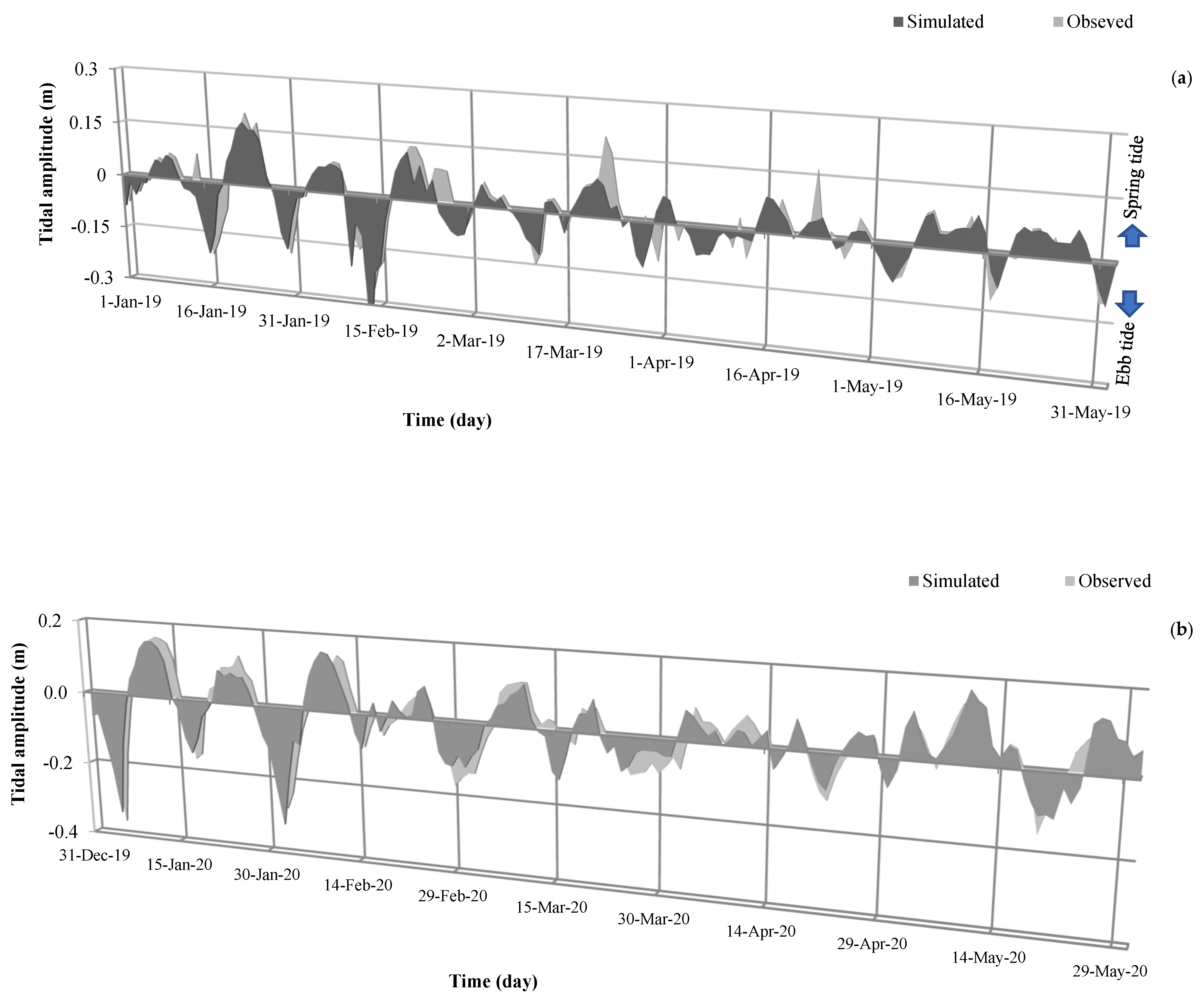
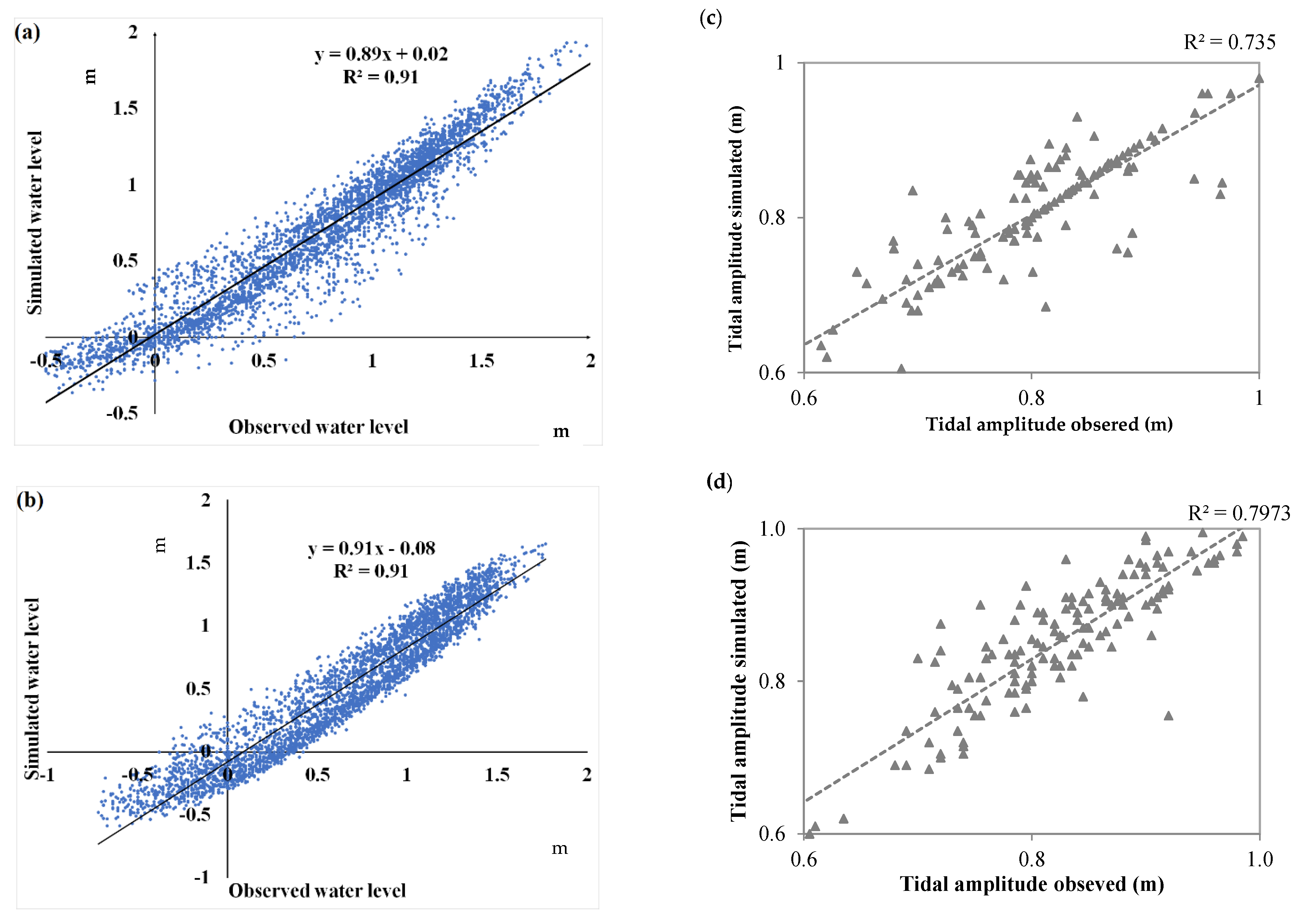
3.1. Calibration and Validation Results of HD Modeling

During the calibration and validation procedure, the Manning’s hydraulic roughness coefficient (n) was found to be 0.03 for the global value (and varied between 0.015 and 0.075 for the local values). The hydrographs of simulated and observed tidal amplitude and water levels in 2019 and 2020 at Long Xuyen station were plotted, and the results are shown in Figure 4 and Figure A1, respectively, whilst, the accuracy of the hydrodynamic model is reported in

Table 3. Summary of correlation coefficient (R), Nash–Sutcliffe efficiency (NSE) and root mean square error (RMSE) of water levels in the dry season (Jan–May) in 2019 and 2020 at Long Xuyen station.

	Time	2019			2020
		NSE	RMSE	R	NSE	RMSE	R
Water level	January	0.90	0.15	0.96	0.85	0.20	0.94
	February	0.88	0.18	0.96	0.85	0.20	0.96
	March	0.88	0.18	0.95	0.84	0.21	0.96
	April	0.87	0.18	0.95	0.84	0.22	0.96
	May	0.89	0.17	0.95	0.86	0.21	0.95
	Jan–May	0.89	0.17	0.95	0.85	0.21	0.96
Tidal amplitude	Jan–May	0.89	0.04	0.73	0.71	0.05	0.79

. Overall, the model’s NSE, R and RMSE values were in the range of 0.84–0.90, 0.94–0.96 and 0.15–0.22 for water level performance, respectively. This indicates the model’s overall good performance. While the 2019 calibration performed better than the 2020 validation, the NSE value for 2019 is 0.89, compared to 0.85 in 2020, and the RMSE value for 2019 (0.17) is likewise lower than that of 2020 (0.21). During this time, the river morphology, river network, the number of dykes and the sluice systems all changed slightly. In 2019, the comparison of tidal amplitudes performed quite well, with 0.89, 0.73 and 0.04 for NSE, R and RMSE, respectively. The results for tidal amplitude tide verification in 2020 were 0.71, 0.79 and 0.05 for NSE, R and RMSE, respectively. The average tidal amplitude at the Long Xuyen station was 0.8, and varied from 0.52 m to 1 m in 2019. In 2020, the tidal average amplitude was 0.85, and varied from 0.49 m to 1 m. According to research by Phan (2019) [50], which revealed that the tidal amplitude in the East Sea of Vietnam fluctuates approximately less than 1.5 m., and that the tidal amplitude in the river tends to decrease compared that of the coast, this is also consistent with the study of Gagliano (1968) [51]. In addition, the correlation between the observed and simulated water levels and the tidal amplitudes showed strong agreement, as seen in Figure 5. This suggests that the developed HD module has a good performance and can be used for further simulation activities.

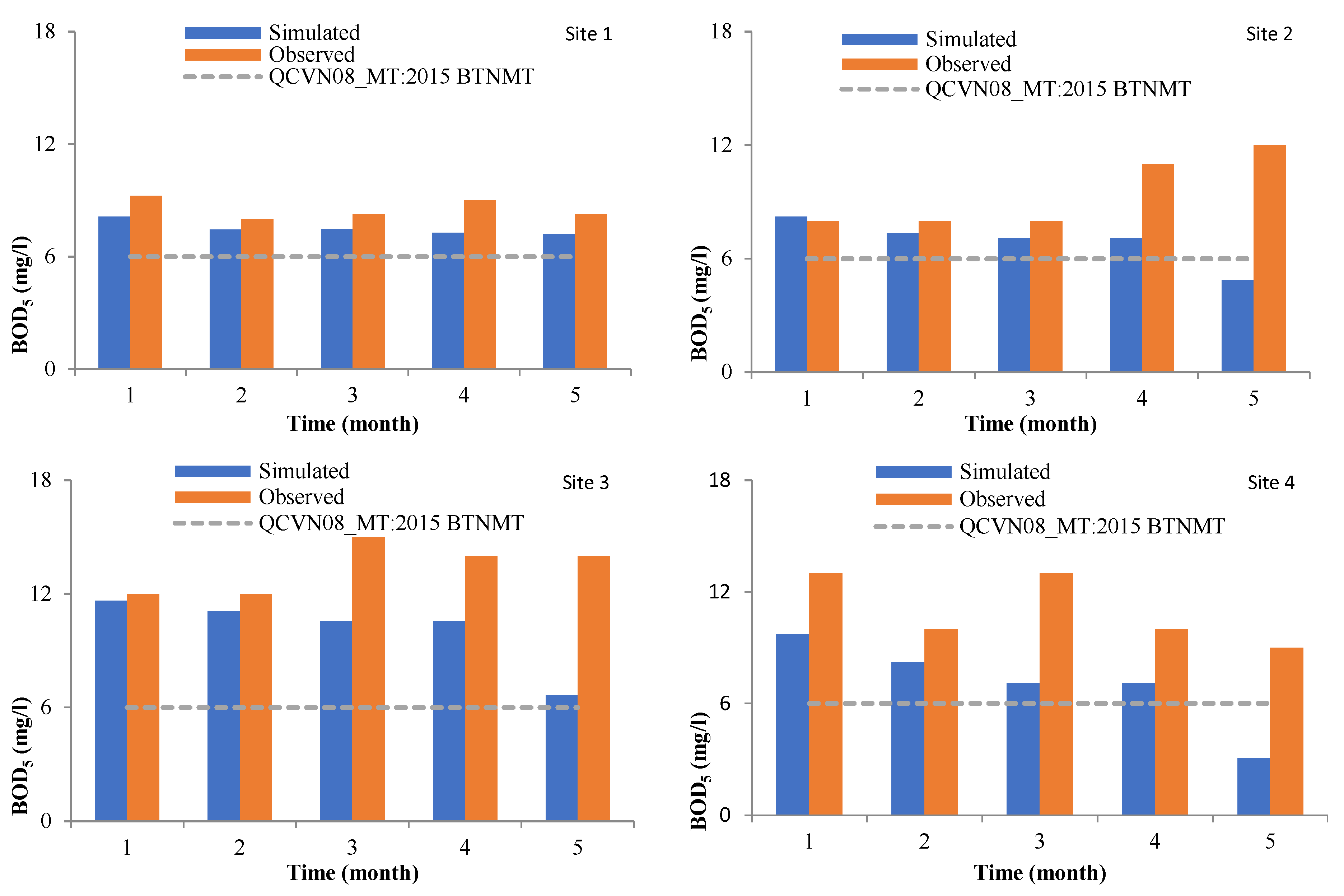
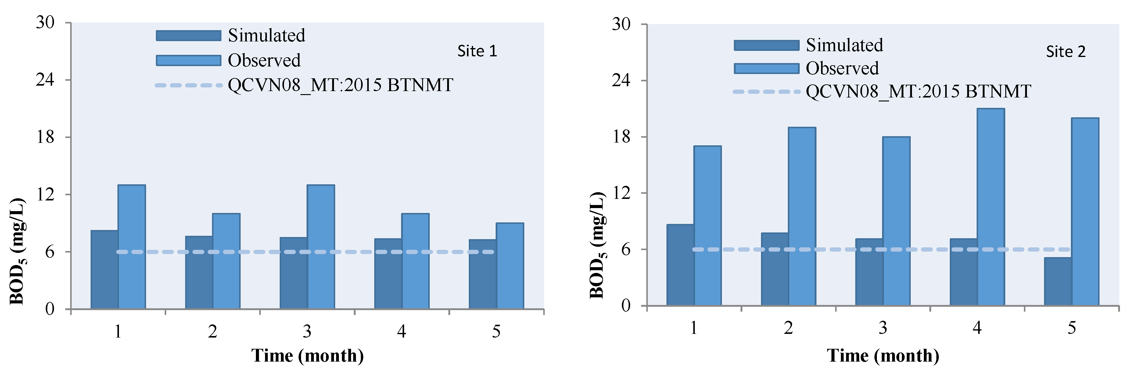
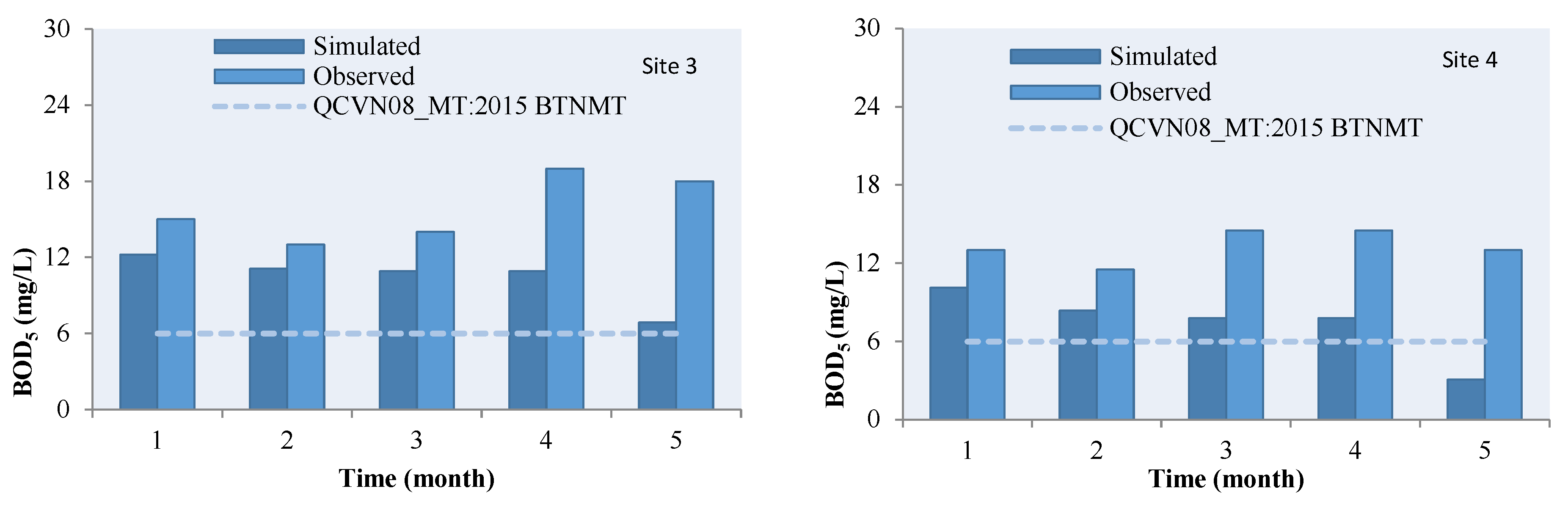
3.2. Calibration and Validation Results of Water Quality Modeling

The EcoLab module is linked to the advection–dispersion (AD) module, which describes both the transformation and transport processes of pollutants. Therefore, the relationship between BOD₅ and DO in different conditions can be used to describe the fluvial water quality. In the calibration step, the dispersion coefficients were seen to vary between 50 and 700, and BOD decay between 0.1 and 1.5. Figure 6 illustrates that the BOD₅ concentration difference between simulated and observed data varies by about 12 percent, 22 percent, 24 percent and 37 percent for first, second, third and fourth sites, respectively. The observed BOD₅ data of the first site were highest, while the accuracy of the fourth site was lowest. The lack of statistics on pollution load at site 4 is due to its proximately to Vinh Te Canal, which forms the boundary between Vietnam and Cambodia.

The simulation findings of water quality metrics demonstrate that the trend for temporal variation for the pollutants were similar between the main river channels and the smaller rivers and canals. The validation results of BOD₅ concentration are shown in Figure 7.

For the first, second, third and fourth sites, the errors between the simulated and observed data were 30 percent, 62 percent, 32 percent and 44 percent, respectively. The accuracy of the first location was the highest, while the accuracy of the second locality was the lowest. Rapid riverbank and riverbed erosion and sedimentation in the research area has led to recent changes in the slope and cross-section of rivers and canals. Moreover, at site no. 2, as well as sites 3 and 4, located in the canal with low discharge volumes, the immediate pollution concentration is often strongly affected directly by the discharge source. In site no. 1, on the main river channel, a much higher discharge volume resulted in quicker pollution dilution, while pollutant concentrations fluctuated less in small canals.

The water quality model performed DO concentrations are in good agreement with the observed DO concentrations in 2019 and 2020 (Figure A2). For the first, second, third and fourth sites, the difference between simulated and observed DO values, respectively, varied by about 14 percent, 11 percent, 14 percent and 13 percent in 2019, and 7 percent, 13 percent, 12 percent and 10 percent in 2020.

An ANOVA was used to further analyze water quality data, i.e., BOD₅, DO and temperature, at stations along the Bassac River, infield canals and aquacultural site canals for the years 2019 and 2020. The aquacultural regions had the highest average BOD₅ (12.88 mg/L), followed by the infield canals (11.55 mg/L) and the Bassac River (9.07 mg/L) in 2019. The difference between BOD₅ in aquaculture and BOD₅ in the Bassac River, on the other hand, was only detected at a 5% significance level in the study. In the aquacultural area, the typical DO and temperature were around 4 mg/L and 30°C, respectively. At a 5% significance level, the aquacultural area’s average DO (4.47 mg/L) and temperature (29.78°C) in 2020 differed from the river’s average DO (5.04 mg/L) and temperature (29.08°C). The aquatic region had the lowest BOD₅ (13.65 mg/L), while the Bassac River (15.47 mg/L) and the infield canals (15.17 mg/L) displayed the highest. We found that water pollution, such as BOD₅ concentrations in the year of 2020, was lower than in the year of 2019. We suspect the reason is due to the impact of the COVID-19 pandemic, leading to decreased fish production and resulting in a decreased BOD₅ load.

However, according to QCVN 08-MT: 2015/BTNMT, column A2 of the National Technical Regulation on surface water quality, the surface water quality deterioration by aquaculture in 2019 and 2020 found in this study was far in exceedance of the desired water quality threshold. The DO concentration of water, for instance, was lower than the QCVN 08 threshold. Hence, when utilizing this water for domestic purposes, it is advised that people pretreat it carefully before use to ensure no long-term adverse health effects. This water quality model may be used by key stakeholders to forecast water quality in the aquacultural area so that appropriate in situ water treatment measures can be located and implemented. Furthermore, numerous studies have revealed transboundary environmental degradation caused by the Mekong River’s flow through two major tributaries, the Mekong River and the Bassac River. The result highlights the need for surface water quality control checks in border areas.

Figure 8 shows the spatial distribution of BOD₅ max, BOD₅ min and BOD₅ max–BOD₅ min. The parameters are highest in the northwest and decrease gradually towards the southeast. High BOD₅ levels can be found in both Chau Doc and Tri Ton. Chau Doc is an urban area bordering Cambodia with moderate tourism activities. The main sources of wastewater in Chau Doc are from urban areas and tourism (average BOD₅ max and BOD₅ min concentrations are 25 mg/L and 17 mg/L, respectively). The population density in Chau Doc and the larger city of Long Xuyen was 963 and 2368 people per square kilometer in the year 2020, respectively. The remaining urban areas, particularly in Kien Giang province, have vastly lower population densities, whilst the impacts of urbanization on fluvial water quality remain minimal in coastal areas. Water quality in and around Long Xuyen is heavily affected not only by production activities, but also by waste from urban residential areas. Tri Ton, a semi-mountainous area in An Giang, is a popular tourist destination that is also undergoing rapid urbanization. Here, moderate levels of water quality were recorded, with the main source of pollution load being from surrounding aquacultural activities. Here, averages of BOD₅ max and BOD₅ min were 16 mg/L and 12 mg/L, respectively. However, on the main river (Bassac River) and inland canals, BOD₅ max was 17 mg/L and 13 mg/L, respectively. Aquacultural practices in the area to the north of Bassac River are typically in the form of in-river cage culture farming, while to the south, aquacultural production is typically practiced in ponds and lagoons. Overall, our results showed that the areas on or directly adjacent to the main river channels showed more variability due to the influence of higher flow volumes and exhibit, therefore, a better self-cleaning capacity [2,3]. Furthermore, according to Minh et al. [2,42], high pollution levels in the Vinh Te Canal have a degrading impact on the wider study area.

High DO levels were found in the main river (Bassac) and main canals (Vinh Te Canal), while DO₅ max–DO₅ min, on the other hand, tends to follow the northwest direction (Figure 9).

4. Discussion

Since the Streeter and Phelps model [52], more than a hundred further water quality models have been developed. The surface water quality models have progressed through many major stages, from assessing a single factor of water quality to multiple factors of water quality, from steady- to non-steady-state hydraulic models, from a point source model to a coupling-model of point and nonpoint sources and from one-dimensional to two-dimensional and three-dimensional models [53,54].

MIKE 11 is an advanced model with water quality management capabilities [55]. According to several studies, MIKE 11 necessitates a large amount of data and, in the case of using a small time step to ensure the stability of the model, simulation step takes a long time [56]. However, MIKE 11 also allows the user to select a simpler model that is appropriate for the target and dataset available. The EcoLab module, in particular, provides six different levels of conceptual water quality modeling complexity.

Moreover, some challenges remain, as models typically require a large amount of accurate data, an absence of which may result in a significant difference between the reality and the simulation results. Further, models do not include pollutant mechanisms, and are ambiguous about contaminant migration, meaning that we cannot predict how contaminants will migrate. Combination models are becoming popular for water quality modeling due to the complexity of water quality issues. In the case of water quality modeling, these models include combination models, artificial intelligence models and system integration [55].

In this study, MIKE 11 provided good results for the hydrodynamics simulation because the input data for the study area was of a high temporal resolution (hourly). However, the water quality monitoring data consisted of only monthly averages. As such, changes in water quality were not clearly visible. The use of an Artificial Neural Network (ANN) to overcome this limitation produced significantly better results than hydrodynamics and water quality modeling, as evidenced by goodness-of-fit indices. The ANN model, developed by McCulloch [57], consists of three layers, and the number of layer increases with the complexity. The ANN model has been used to predict some key water quality parameters in recent years, with results indicating that its accuracy is adequate for practical purposes.

Previous research also suggests that the ANN performs better in predicting water level, as well as nitrate and phosphate, compared to Support Vector Machine models [58,59]. Moreover, Rabindra et al. reveal that ANN does not require other physical parameters in the modeling process, which can reduce the complexities of modeling the system [60]. Most numerical models, on the other hand, have not been fully validated against field experimental data, which often requires large investments of time and capital to obtain. Data-based models have been used to replace the numerical model because water quality predictions can be made using only accumulated data. The ANN is one of many data-driven techniques that has been widely applied due to its efficiency in predicting and forecasting water quantity and quality variables in river systems [61].

5. Conclusions

The hydrodynamics module developed in this study was calibrated and validated to be in good agreement with the observed data. After successful flow simulation, the AD and EcoLab modules of MIKE 11 were used to simulate the surface water quality of the LXQ using discharge and water level data from existing the HD module in the dry season. The results of the BOD₅ transmission simulation meet the practical needs of the study area by assisting the appropriate management and planning of aquacultural areas in order to reduce pollution and the impact of harmful chemicals from other sources

High BOD₅ pollution was seen in most pond and lagoon aquacultural sites during the dry season in both 2019 and 2020. This is because ponds and lagoons have frequently slower growth stages, are less well ventilated than cage freshwater rearing areas, with limited water exchange and self-cleaning. However, the areas close to cage culture farming areas were found to have higher BOD₅ than areas surrounding pond/lagoon culture. The reason is due to the influences from other point pollution sources, such as upstream wastewater urban and tourism areas. Therefore, before locating and promoting aquacultural production, it is necessary to test site water quality. Furthermore, aquacultural areas should be located and zoned far from urban and tourist areas. Overall, the management and effective sustainable use of water resources needs to be strengthened to ensure the overall suitability of aquacultural locations.

Additionally, considering the data scarcity, several automatic measurement stations are proposed to aid the understanding of the spatio-temporal dynamics of water quality parameters, as well as data for improved model calibration and verification. Furthermore, diligent monitoring of all important hydrogeochemical parameters, such as salinity, isotopes/tracer elements, etc., which help in deciphering the seawater–freshwater mixing mechanisms in this dynamic hydrological system, should be considered as a future course of work.

References

1. Duc, N.H.; Avtar, R.; Kumar, P.; Lan, P.P. Scenario-Based Numerical Simulation to Predict Future Water Quality for Developing Robust Water Management Plan: A Case Study from the Hau River, Vietnam. Mitig. Adapt. Strateg. Glob. Chang. 2021, 26, 33. [Google Scholar] [CrossRef]
2. Thu Minh, H.V.; Avtar, R.; Kumar, P.; Le, K.N.; Kurasaki, M.; Ty, T.V. Impact of Rice Intensification and Urbanization on Surface Water Quality in An Giang Using a Statistical Approach. Water 2020, 12, 1710. [Google Scholar] [CrossRef]
3. Minh, H.V.T.; Kurasaki, M.; Ty, T.V.; Tran, D.Q.; Le, K.N.; Avtar, R.; Rahman, M.M.; Osaki, M. Effects of Multi-Dike Protection Systems on Surface Water Quality in the Vietnamese Mekong Delta. Water 2019, 11, 1010. [Google Scholar] [CrossRef] [Green Version]
4. Vörösmarty, C.J.; McIntyre, P.B.; Gessner, M.O.; Dudgeon, D.; Prusevich, A.; Green, P.; Glidden, S.; Bunn, S.E.; Sullivan, C.A.; Liermann, C.R.; et al. Global Threats to Human Water Security and River Biodiversity. Nature 2010, 467, 555. [Google Scholar] [CrossRef] [PubMed]
5. Eng, C.T.; Paw, J.N.; Guarin, F.Y. The Environmental Impact of Aquaculture and the Effects of Pollution on Coastal Aquaculture Development in Southeast Asia. Mar. Pollut. Bull. 1989, 20, 335–343. [Google Scholar]
6. Schneider, P.; Asch, F. Rice Production and Food Security in Asian Mega Deltas—A Review on Characteristics, Vulnerabilities and Agricultural Adaptation Options to Cope with Climate Change. J. Agron. Crop Sci. 2020, 206, 491–503. [Google Scholar] [CrossRef]
7. Berg, H.; Tam, N.T. Use of Pesticides and Attitude to Pest Management Strategies among Rice and Rice-Fish Farmers IntheMekong Delta, Vietnam. Int. J. Pest Manag. 2012, 58, 153–164. [Google Scholar] [CrossRef]
8. Anh, P.T.; Kroeze, C.; Bush, S.R.; Mol, A.P. Water Pollution by Pangasius Production in the Mekong Delta, Vietnam: Causes and Options for Control. Aquac. Res. 2010, 42, 108–128. [Google Scholar] [CrossRef]
9. Mutea, F.G.; Nelson, H.K.; Au, H.V.; Huynh, T.G.; Vu, U.N. Assessment of Water Quality for Aquaculture in Hau River, Mekong Delta, Vietnam Using Multivariate Statistical Analysis. Water 2021, 13, 3307. [Google Scholar] [CrossRef]
10. Bouman, B.A.M.; Tuong, T.P. Field Water Management to Save Water and Increase Its Productivity in Irrigated Lowland Rice. Agric. Water Manag. 2001, 49, 11–30. [Google Scholar] [CrossRef]
11. Giao, N.T. Surface Water Quality in Aquacultural Areas in An Giang Province, Vietnam. Int. J. Environ. Agric. Biotechnol. 2020, 5, 1054–1061. [Google Scholar] [CrossRef]
12. Ndikumana, E.; Ho Tong Minh, D.; Dang Nguyen, T.H.; Baghdadi, N.; Courault, D.; Hossard, L.; El Moussawi, I. Estimation of Rice Height and Biomass Using Multitemporal SAR Sentinel-1 for Camargue, Southern France. Remote Sens. 2018, 10, 1394. [Google Scholar] [CrossRef] [Green Version]
13. Phung, D.; Huang, C.; Rutherford, S.; Dwirahmadi, F.; Chu, C.; Wang, X.; Nguyen, M.; Nguyen, N.H.; Do, C.M.; Nguyen, T.H. Temporal and Spatial Assessment of River Surface Water Quality Using Multivariate Statistical Techniques: A Study in Can Tho City, a Mekong Delta Area, Vietnam. Environ. Monit. Assess. 2015, 187, 229. [Google Scholar] [CrossRef] [PubMed]
14. Dunca, A.-M. Water Pollution and Water Quality Assessment of Major Transboundary Rivers from Banat (Romania). J. Chem. 2018, 2018, 9073763. [Google Scholar] [CrossRef] [Green Version]
15. Ighalo, J.O.; Adeniyi, A.G. A Comprehensive Review of Water Quality Monitoring and Assessment in Nigeria. Chemosphere 2020, 260, 127569. [Google Scholar] [CrossRef] [PubMed]
16. Avtar, R.; Kumar, P.; Singh, C.; Mukherjee, S. A Comparative Study on Hydrogeochemistry of Ken and Betwa Rivers of Bundelkhand Using Statistical Approach. Water Qual. Expo. Health 2011, 2, 169–179. [Google Scholar] [CrossRef]
17. Molekoa, M.D.; Avtar, R.; Kumar, P.; Minh, H.V.T.; Kurniawan, T.A. Hydrogeochemical Assessment of Groundwater Quality of Mokopane Area, Limpopo, South Africa Using Statistical Approach. Water 2019, 11, 1891. [Google Scholar] [CrossRef] [Green Version]
18. Singh, S.; Ghosh, N.; Gurjar, S.; Krishan, G.; Kumar, S.; Berwal, P. Index-Based Assessment of Suitability of Water Quality for Irrigation Purpose under Indian Conditions. Environ. Monit. Assess. 2018, 190, 29. [Google Scholar] [CrossRef] [PubMed]
19. Minh, H.V.T.; Avtar, R.; Kumar, P.; Tran, D.Q.; Ty, T.V.; Behera, H.C.; Kurasaki, M. Groundwater Quality Assessment Using Fuzzy-AHP in An Giang Province of Vietnam. Geosciences 2019, 9, 330. [Google Scholar] [CrossRef] [Green Version]
20. Kumar, P. Numerical Quantification of Current Status Quo and Future Prediction of Water Quality in Eight Asian Megacities: Challenges and Opportunities for Sustainable Water Management. Environ. Monit. Assess. 2019, 191, 319. [Google Scholar] [CrossRef]
21. Kumar, P.; Johnson, B.A.; Dasgupta, R.; Avtar, R.; Chakraborty, S.; Kawai, M.; Magcale-Macandog, D.B. Participatory Approach for More Robust Water Resource Management: Case Study of the Santa Rosa Sub-Watershed of the Philippines. Water 2020, 12, 1172. [Google Scholar] [CrossRef] [Green Version]
22. Kumar, P.; Avtar, R.; Dasgupta, R.; Johnson, B.A.; Mukherjee, A.; Ahsan, M.N.; Nguyen, D.C.H.; Nguyen, H.Q.; Shaw, R.; Mishra, B.K. Socio-Hydrology: A Key Approach for Adaptation to Water Scarcity and Achieving Human Well-Being in Large Riverine Islands. Prog. Disaster Sci. 2020, 8, 100134. [Google Scholar] [CrossRef]
23. Hanington, P.; To, Q.T.; Van, P.D.T.; Doan, N.A.V.; Kiem, A.S. A Hydrological Model for Interprovincial Water Resource Planning and Management: A Case Study in the Long Xuyen Quadrangle, Mekong Delta, Vietnam. J. Hydrol. 2017, 547, 1–9. [Google Scholar] [CrossRef]
24. Liang, J.; Yang, Q.; Sun, T.; Martin, J.; Sun, H.; Li, L. MIKE 11 Model-Based Water Quality Model as a Tool for the Evaluation of Water Quality Management Plans. J. Water Supply Res. Technol. 2015, 64, 708–718. [Google Scholar] [CrossRef] [Green Version]
25. Gedam, V.; Kelkar, P.; Jha, R.; Khadse, G.; Labhasetwar, P. Assessment of Assimilative Capacity of Kanhan River Stretch Using Mike-11 Modeling Tool Using Mike-11 Modeling Tool. J Environ. Sci. Engg. 2012, 54, 481–488. [Google Scholar]
26. Arnold, J.G.; Srinivasan, R.; Muttiah, R.S.; Williams, J.R. Large Area Hydrologic Modeling and Assessment Part I: Model Development. JAWRA J. Am. Water Resour. Assoc. 1998, 34, 73–89. [Google Scholar] [CrossRef]
27. Dang, T.D.; Cochrane, T.A.; Arias, M.E. Future Hydrological Alterations in the Mekong Delta under the Impact of Water Resources Development, Land Subsidence and Sea Level Rise. J. Hydrol. Reg. Stud. 2018, 15, 119–133. [Google Scholar] [CrossRef]
28. Smajgl, A.; Toan, T.Q.; Nhan, D.K.; Ward, J.; Trung, N.H.; Tri, L.; Tri, V.; Vu, P. Responding to Rising Sea Levels in the Mekong Delta. Nat. Clim. Chang. 2015, 5, 167–174. [Google Scholar] [CrossRef]
29. Chinh, P.V. Application of Mathematical Models to Assess Water Quality in the Downstream of Dong Nai River up to 2020. Master thesis. Da Nang University, Da Nang City, Vietnam. 2011. Master’s Thesis, Da Nang University, Da Nang City, Vietnam, 2011. [Google Scholar]
30. Johnston, R.; Kummu, M. Water Resource Models in the Mekong Basin: A Review. Water Resour. Manag. 2012, 26, 429–455. [Google Scholar] [CrossRef]
31. Water Environment Partnership in Asia. Surface Water in Vietnam. State of Water Environmental Issues. Available online: http://www.wepa-db.net/policies/state/vietnam/surface.htm (accessed on 30 March 2021).
32. Kuenzer, C.; Guo, H.; Huth, J.; Leinenkugel, P.; Li, X.; Dech, S. Flood Mapping and Flood Dynamics of the Mekong Delta: ENVISAT-ASAR-WSM Based Time Series Analyses. Remote Sens. 2013, 5, 687–715. [Google Scholar] [CrossRef] [Green Version]
33. Vietnamese Government Resolution No. 120/NQ-CP-Resolution on Sustainable Climate-Resilient Development of the Vietnamese Mekong Delta, Vietnames Government, Vietnam. 2017; Available online: https://english.luatvietnam.vn/resolution-no120-nq-cp-dated-november-17-2017-of-the-government-on-sustainable-and-climate-resilient-development-of-the-mekong-river-delta-118378-Doc1.html (accessed on 18 November 2021).
34. Wilbers, G.-J.; Becker, M.; Nga, L.T.; Sebesvari, Z.; Renaud, F.G. Spatial and Temporal Variability of Surface Water Pollution in the Mekong Delta, Vietnam. Sci. Total Environ. 2014, 485–486, 653–665. [Google Scholar] [CrossRef] [PubMed]
35. Dinh, Q.; Balica, S.; Popescu, I.; Jonoski, A. Climate Change Impact on Flood Hazard, Vulnerability and Risk of the Long Xuyen Quadrangle in the Mekong Delta. Int. J. River Basin Manag. 2012, 10, 103–120. [Google Scholar] [CrossRef]
36. Duc Tran, D.; van Halsema, G.; Hellegers, P.J.G.J.; Phi Hoang, L.; Quang Tran, T.; Kummu, M.; Ludwig, F. Assessing Impacts of Dike Construction on the Flood Dynamics of the Mekong Delta. Hydrol. Earth Syst. Sci. 2018, 22, 1875–1896. [Google Scholar] [CrossRef] [Green Version]
37. Manh, N.V.; Dung, N.V.; Hung, N.N.; Merz, B.; Apel, H. Large-Scale Suspended Sediment Transport and Sediment Deposition in the Mekong Delta. Hydrol. Earth Syst. Sci. 2014, 18, 3033–3053. [Google Scholar] [CrossRef] [Green Version]
38. Le Anh Tuan, C.T.H.; Miller, F.; Sinh, B.T. Flood and Salinity Management in the Mekong Delta, Vietnam. The Sustainable Mekong Research Network (Sumernet): Bangkok, Thailand, 2007; pp. 15–68. [Google Scholar]
39. Balica, S.; Dinh, Q.; Popescu, I.; Vo, T.Q.; Pham, D.Q. Flood Impact in the Mekong Delta, Vietnam. J. Maps 2014, 10, 257–268. [Google Scholar] [CrossRef]
40. DoNRE. An Giang. Summary Report on Environmental Monitoring Results in An Giang Province in 2020; DoNRE: Long Xuyen, Vietnam, 2020; p. 361. [Google Scholar]
41. San Diego-McGlone, M.L.; Smith, S.V.; Nicolas, V.F. Stoichiometric Interpretations of C:N:P Ratios in Organic Waste Materials. Mar. Pollut. Bull. 2000, 40, 325–330. [Google Scholar] [CrossRef]
42. Minh, H.V.T.; Tam, N.T.; Nhu, Đ.T.; Ty, T.V. Assessment of the Surface Water Quality and Effectiveness of Triple-Glutinous Rice Cropping System in the Full–Dike Protected Area of Bac Vam Nao, An Giang Province. Vietnam J. Hydrometeorol. 2021, 732, 38–48. [Google Scholar] [CrossRef]
43. UNEP. Pollutants from Land-Based Sources in the Mediterranean; UNEP Regional Seas Reports and Studies No. 3; UNEP (United Nations Environment Programme): Washingtone DC, USA, 1984; p. 104. [Google Scholar]
44. Le, X.S.; Le, V.N. Load of Pollutions onto Da Nang Bay. J. Mar. Sci. Technol. 2015, 15, 165–175. [Google Scholar] [CrossRef] [Green Version]
45. Mai, T.H.; Ngô, X.N.; Trần, V.T.; Mai, T.H. Research to Determine Pollutant Load into Truong Giang River, Quang Nam Province. J. Clim. Change Science 2018, 34, 71–79. [Google Scholar]
46. Dung, N.V.; Merz, B.; Bárdossy, A.; Thang, T.D.; Apel, H. Multi-Objective Automatic Calibration of Hydrodynamic Models Utilizing Inundation Maps and Gauge Data. Hydrol. Earth Syst. Sci. 2011, 15, 1339–1354. [Google Scholar] [CrossRef] [Green Version]
47. Saito, Y.; Nguyen, V.L.; Ta, T.K.O.; Tamura, T.; Kanai, Y.; Nakashima, R. Tide and River Influences on Distributary Channels of the Mekong River Delta; American Geophysical Union: Washington, DC, USA, 2015; Volume 2015, p. GC41F-1148. [Google Scholar]
48. Wolanski, E.; Huan, N.N.; Nhan, N.H.; Thuy, N.N. Fine-Sediment Dynamics in the Mekong River Estuary, Vietnam. Estuar. Coast. Shelf Sci. 1996, 43, 565–582. [Google Scholar] [CrossRef]
49. Moriasi, D.N.; Arnold, J.G.; Van Liew, M.W.; Bingner, R.L.; Harmel, R.D.; Veith, T.L. Model Evaluation Guidelines for Systematic Quantification of Accuracy in Watershed Simulations. Trans. ASABE 2007, 50, 885–900. [Google Scholar] [CrossRef]
50. Phan, H.M.; Ye, Q.; Reniers, A.J.; Stive, M.J. Tidal Wave Propagation along The Mekong Deltaic Coast. Estuar. Coast. Shelf Sci. 2019, 220, 73–98. [Google Scholar] [CrossRef]
51. Gagliano, S.; McIntire, W. Reports on the Mekong Delta; Technical Report; Louisiana State University Coastal Studies Institute: Baton Rouge, LA, USA, 1968; Volume 57. [Google Scholar]
52. Wang, Q.; Li, S.; Jia, P.; Qi, C.; Ding, F. A Review of Surface Water Quality Models. Sci. World J. 2013, 2013, 231768. [Google Scholar] [CrossRef] [Green Version]
53. Wang, Q.; Zhao, X.; Yang, M.; Zhao, Y.; Liu, K.; Ma, Q. Water Quality Model Establishment for Middle and Lower Reaches of Hanshui River, China. Chin. Geogr. Sci. 2011, 21, 646–655. [Google Scholar] [CrossRef]
54. Burn, D.H.; McBean, E.A. Optimization Modeling of Water Quality in an Uncertain Environment. Water Resour. Res. 1985, 21, 934–940. [Google Scholar] [CrossRef]
55. Gao, L.; Li, D. A Review of Hydrological/Water-Quality Models. Front. Agric. Sci. Eng. 2015, 1, 267–276. [Google Scholar] [CrossRef] [Green Version]
56. Cox, B. A Review of Currently Available In-Stream Water-Quality Models and Their Applicability for Simulating Dissolved Oxygen in Lowland Rivers. Sci. Total Environ. 2003, 314, 335–377. [Google Scholar] [CrossRef]
57. McCulloch, W.S.; Pitts, W. A Logical Calculus of the Ideas Immanent in Nervous Activity. Bull. Math. Biophys. 1943, 5, 115–133. [Google Scholar] [CrossRef]
58. Stamenković, L.J. Application of ANN and SVM for Prediction Nutrients in Rivers. J. Environ. Sci. Health Part A 2021, 56, 867–873. [Google Scholar] [CrossRef]
59. Cuong, N.P.; Ty, T.V.; An, T.V.; Minh, H.V.T. Application of Artificial Neural Network (ANN) to Predict Water Levels for Urban Inundation Prediction in Can Tho City. Agric. Rural Dev. J. 2019, 1, 53–60. [Google Scholar]
60. Panda, R.K.; Pramanik, N.; Bala, B. Simulation of River Stage Using Artificial Neural Network and MIKE 11 Hydrodynamic Model. Comput. Geosci. 2010, 36, 735–745. [Google Scholar] [CrossRef]
61. Maier, H.R.; Dandy, G.C. The Use of Artificial Neural Networks for the Prediction of Water Quality Parameters. Water Resour. Res. 1996, 32, 1013–1022. [Google Scholar] [CrossRef]
Figure 1. Map of the Vietnamese Mekong Delta and the Long Xuyen Quadrangle (LXQ) with its upstream and downstream boundaries. Calibration and validation samples were collected in the provinces of An Giang, Kien Giang and Can Tho. Long Xuyen Canal = 1, Vinh Tre Canal = 2, Rac Gia-Long Xuyen Canal = 3 and Tam Ngan Canal = 4.
Water 14 00412 g001
Figure 2. The hydrodynamics and water quality modeling procedure phases utilizing one-dimensional MIKE 11.
Water 14 00412 g002
Figure 3. The river and canal network in the LXQ. Blue squares denote the HD (discharge in the upstream and water levels in the downstream) and EcoLab (BOD5, DO and temperature) boundaries.
Water 14 00412 g003
Figure 4. Time series of daily simulated and observed amplitudes in both 2019 (a) and 2020 (b) at Long Xuyen station.
Water 14 00412 g004
Figure 5. The correlation plots between observed and simulated water level data at an hourly scale for the dry seasons in (a) 2019 and (b) 2020. The correlation plots between observed and simulated tidal amplitude at a daily scale for the dry seasons in (c) 2019 and (d) 2020.
Water 14 00412 g005
Figure 6. Calibrated results of BOD5 concentration at the four sites within the study area for the year 2019. The National Technical Regulation on surface water quality (QCVN 08MT:2015) was approved by the Ministry of Environment and Natural Resources (MoNRE) in 2015.
Water 14 00412 g006
Figure 7. Validated results of BOD5 concentration at the four locations within the study area for the year 2020.
Water 14 00412 g007aWater 14 00412 g007b
Figure 8. BOD5 concentration in the dry season of 2020. Here, (ac) represent the maximum, minimum and the difference between the maximum and minimum BOD5 concentration values, respectively. Moreover, (a, b) also show the location of urban and tourism areas, and provincial boundaries. These arrows show the downtrends of BOD5 concentration (a, b) and the downtrends of BOD5 max–BOD5 min.
Water 14 00412 g008aWater 14 00412 g008b
Figure 9. DO concentration in the dry season of 2020. Here, (ac) represent the maximum, minimum and difference between the maximum and minimum DO concentration values, respectively. These arrows show the downward trend of DO concentration (9a,9b) and the downward trend of DO max–DO min.
Water 14 00412 g009aWater 14 00412 g009b