
Dynamic Roughness Modeling of Seasonal Vegetation Effect: Case Study of the Nanakita River
 , ,
, ,
Abstract
:1. Introduction
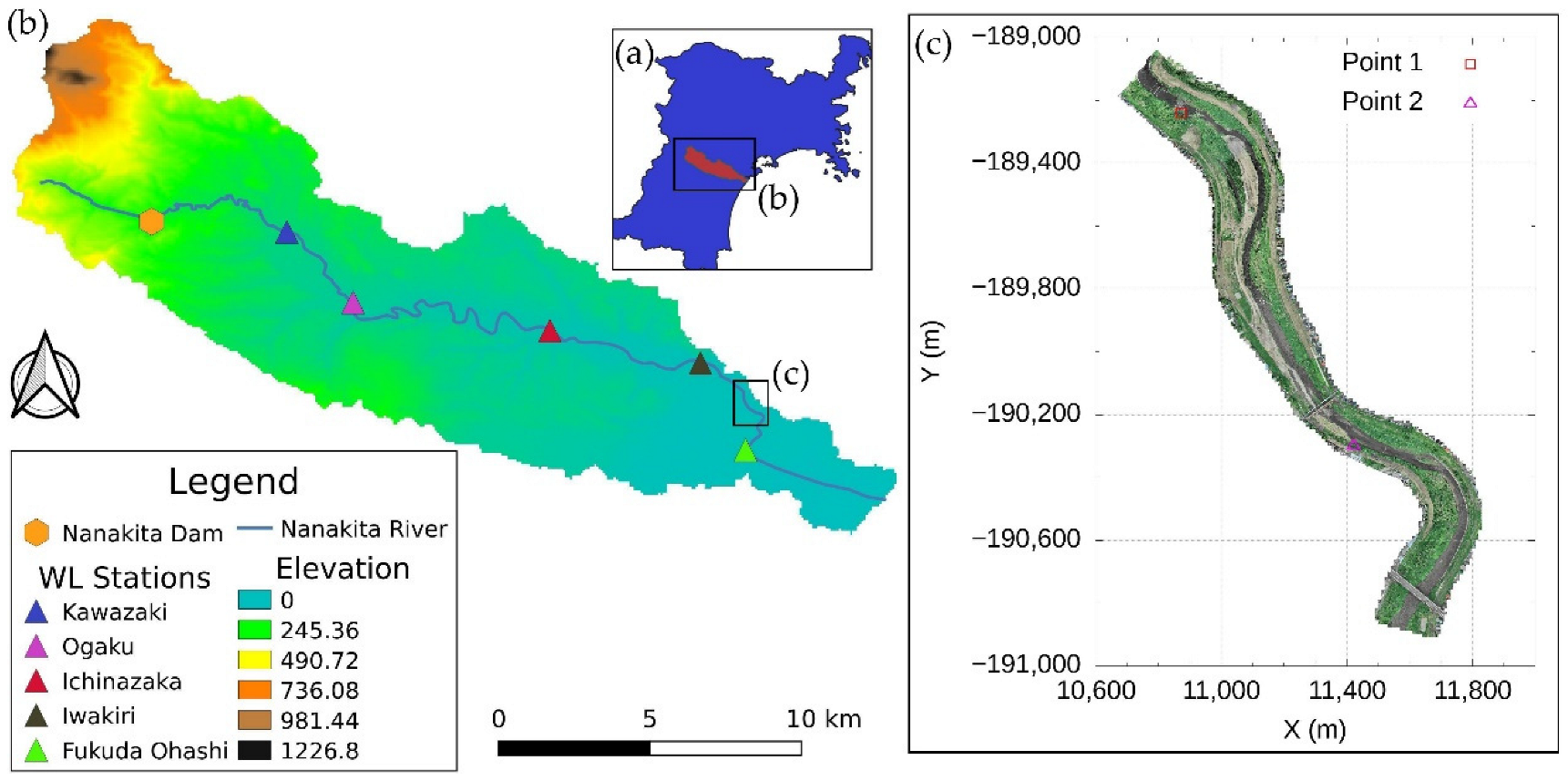
2. Study Area
3. Methodology
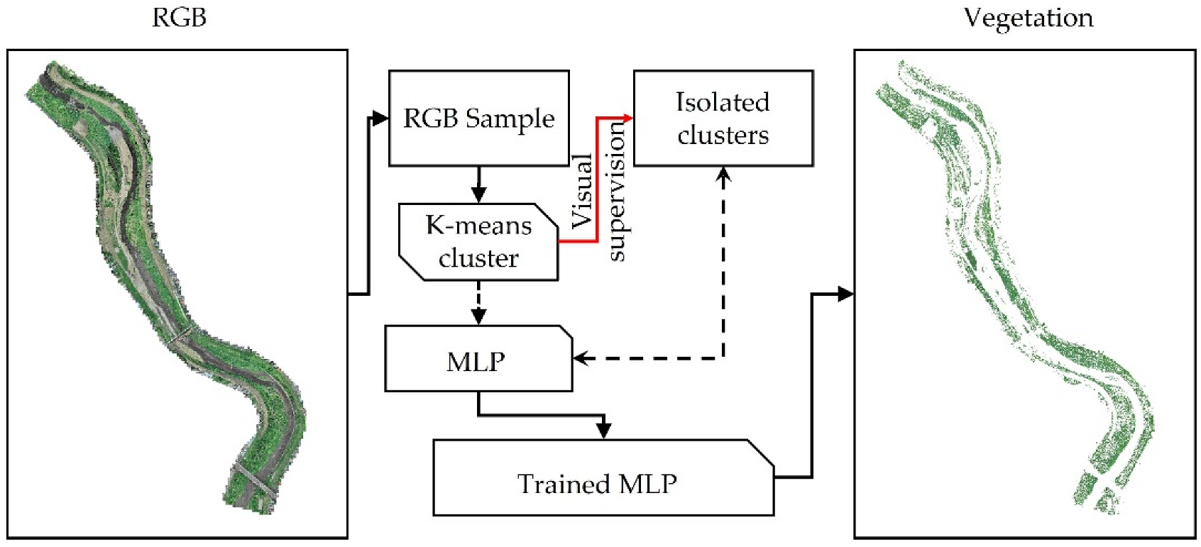
3.1. UAV Observations
3.2. Hydrologic Model
3.3. Two-Dimensional Hydraulic Model
3.4. Dynamic Roughness
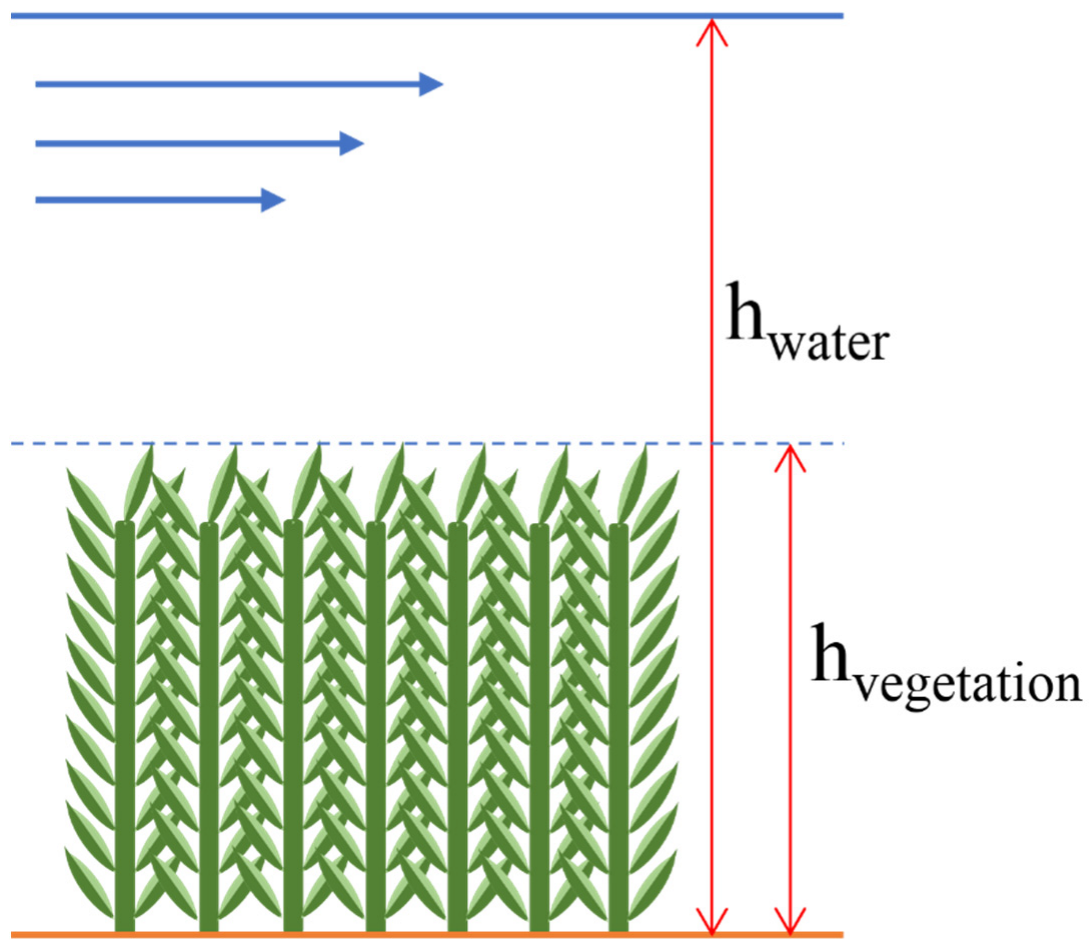
3.5. Vegetation Characteristics
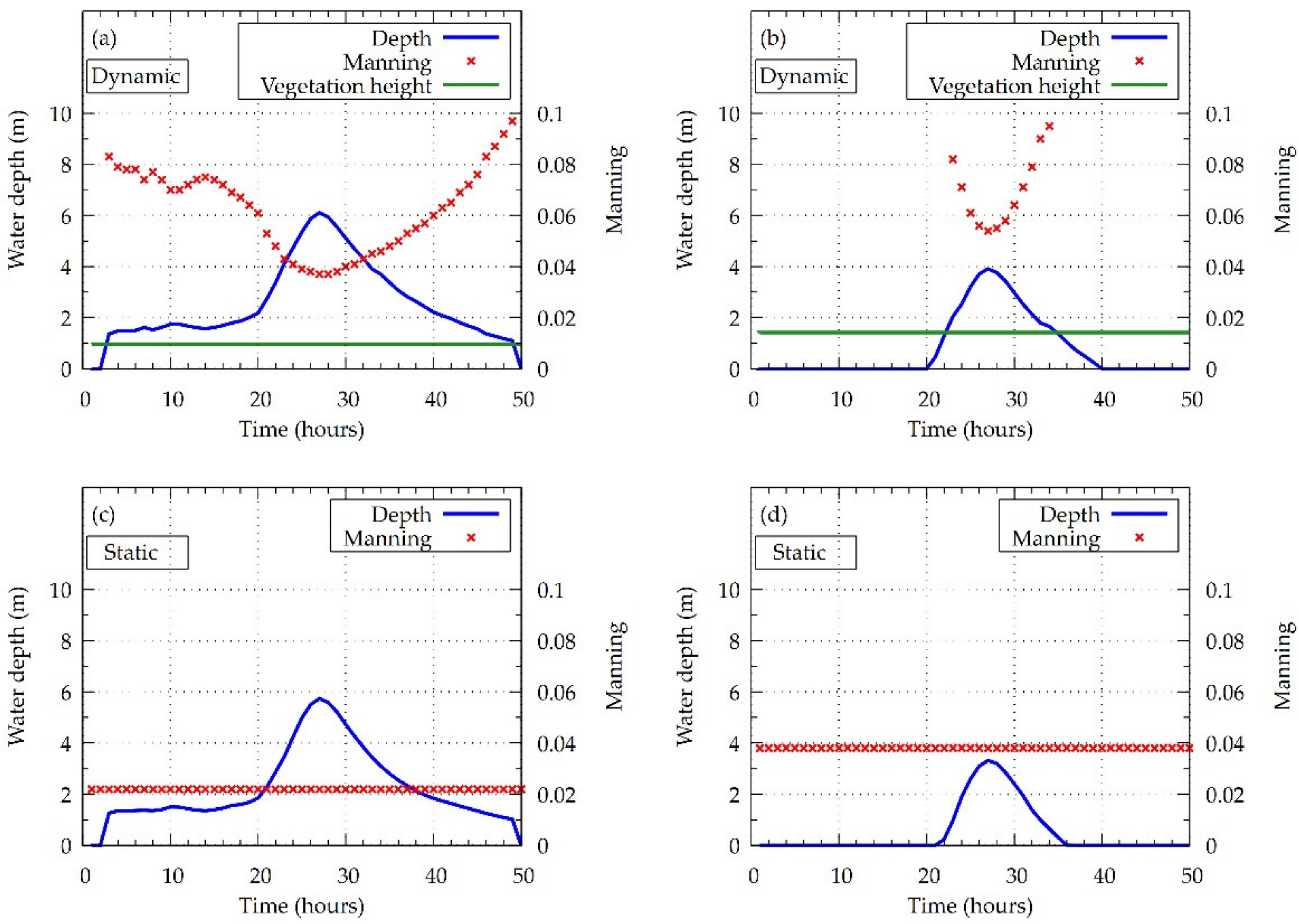
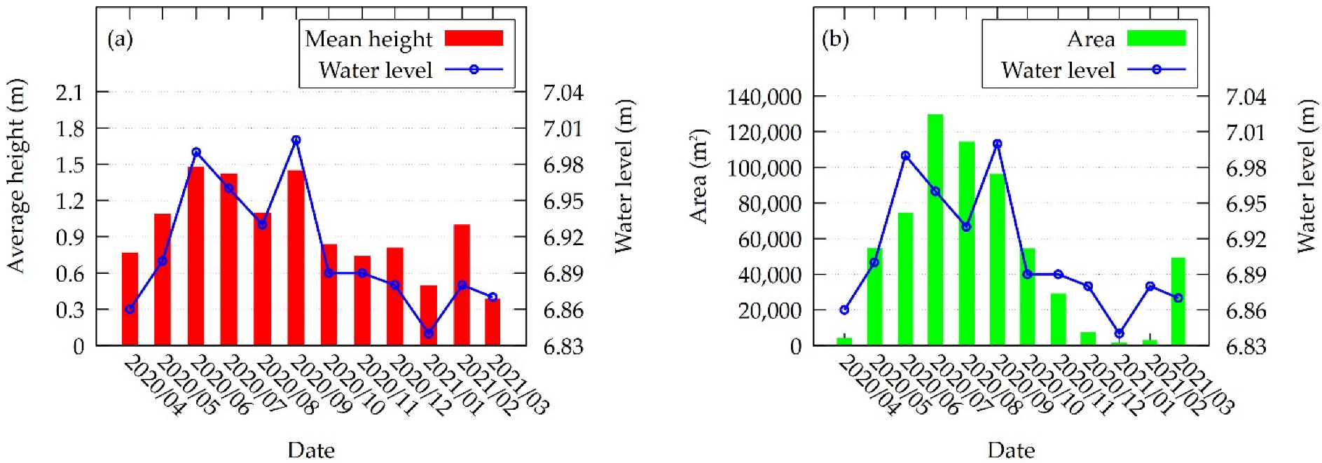
4. Results and Discussion
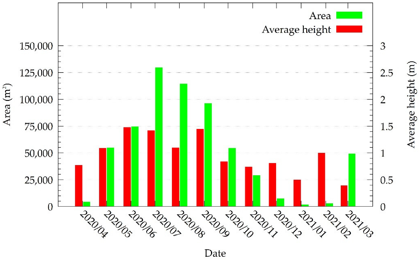
4.1. Vegetation Conditions
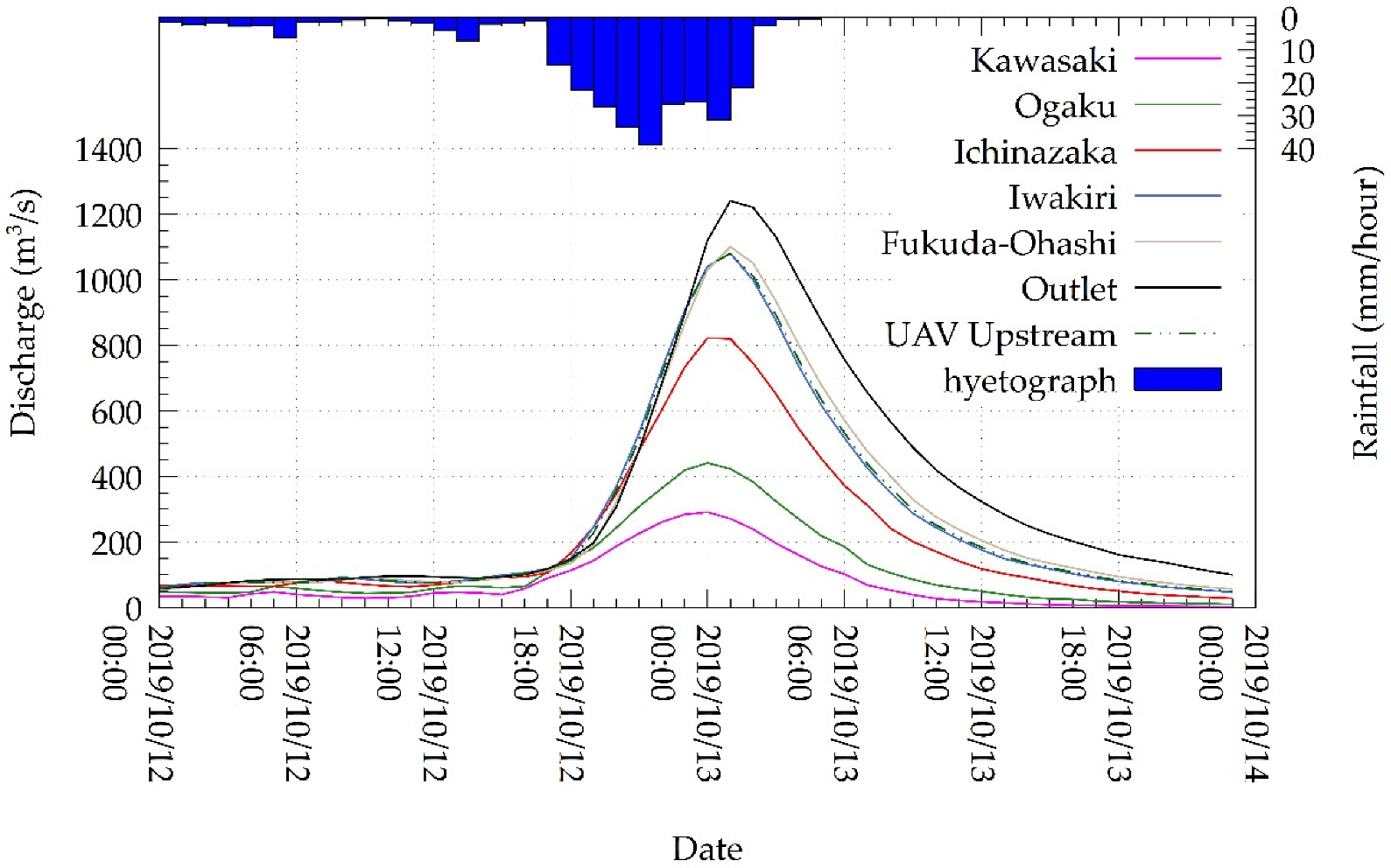
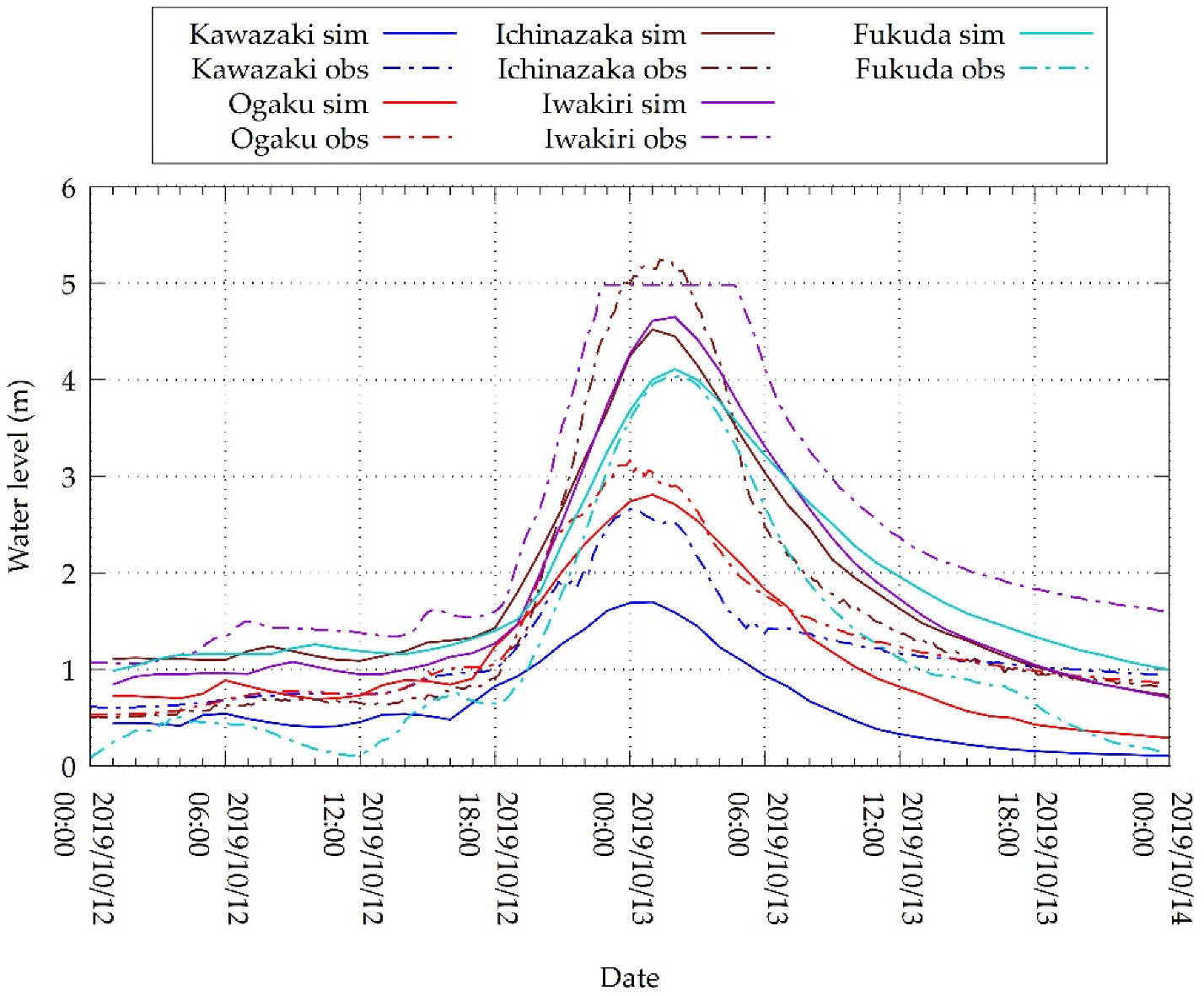
4.2. Hydrologic Simulation
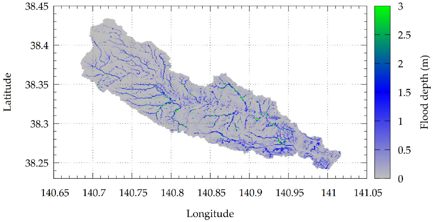
4.3. Hydraulic Simulation
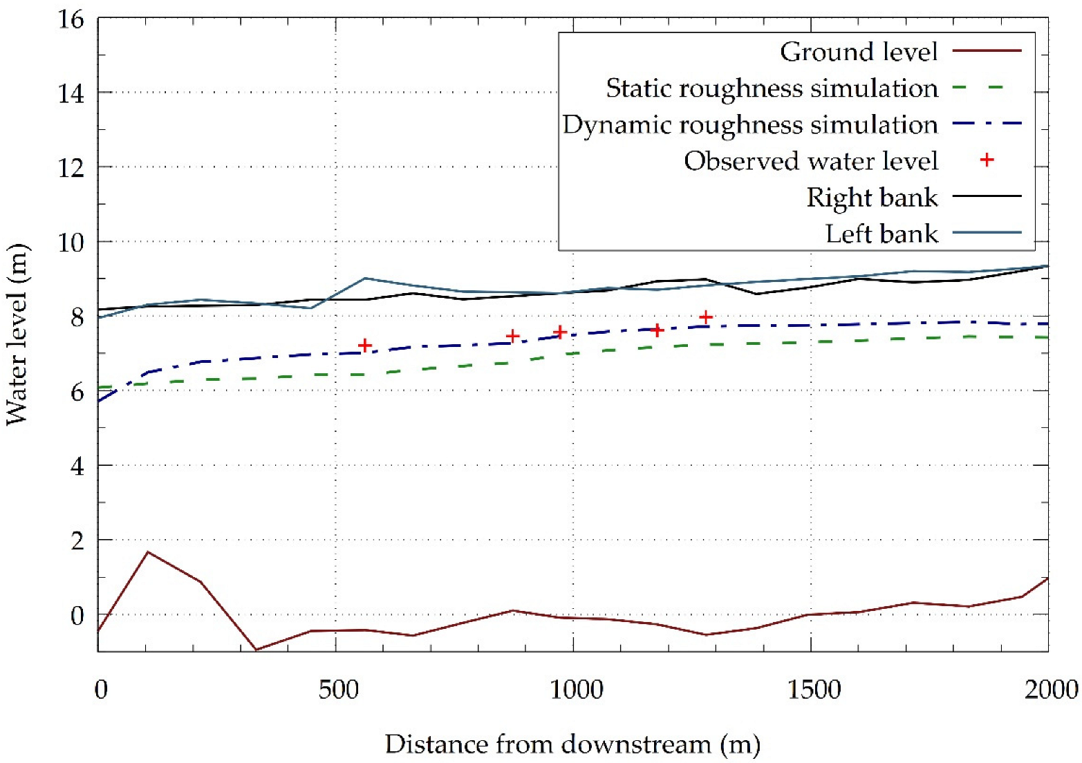
4.4. Seasonal Effect of Vegetation on the Water Profile
5. Conclusions
Author Contributions
Funding
Institutional Review Board Statement
Informed Consent Statement
Data Availability Statement
Acknowledgments
Conflicts of Interest
References
- Cowan, W.L. Estimating hydraulic roughness coefficients. Agric. Eng. 1956, 37, 473–475. [Google Scholar]
- Ebrahimi, N.G.; Fathi-Moghadam, M.; Kashefipour, S.M.; Saneie, M.; Ebrahimi, K. Effects of flow and vegetation states on river roughness coefficients. J. Appl. Sci. 2008, 8, 2118–2123. [Google Scholar] [CrossRef] [Green Version]
- Darby, S.E. Effect of riparian vegetation on flow resistance and flood potential. J. Hydraul. Eng. 1999, 125, 443–454. [Google Scholar] [CrossRef]
- Sun, X.; Shiono, K.; Rameshwaran, P.; Chandler, J.H. Modelling vegetation effects in irregular meandering river. J. Hydraul. Res. 2010, 48, 775–783. [Google Scholar] [CrossRef]
- Nikora, V.; Larned, S.; Nikora, N.; Debnath, K.; Cooper, G.; Reid, M. Hydraulic resistance due to aquatic vegetation in small streams: Field study. J. Hydraul. Eng. 2008, 134, 1326–1332. [Google Scholar] [CrossRef]
- Wang, P.; Wang, C.; Zhu, D.Z. Hydraulic resistance of submerged vegetation related to effective height. J. Hydrodynam. 2010, 22, 265–273. [Google Scholar] [CrossRef]
- Wilson, C.A.M.E. Flow resistance models for flexible submerged vegetation. J. Hydrol. 2007, 342, 213–222. [Google Scholar] [CrossRef]
- Wu, F.-C.; Shen, H.W.; Chou, Y.-J. Variation of roughness coefficients for unsubmerged and submerged vegetation. J. Hydraul. Eng. 1999, 125, 934–942. [Google Scholar] [CrossRef] [Green Version]
- Devi, T.B.; Kumar, B. Experimentation on submerged flow over flexible vegetation patches with downward seepage. Ecol. Eng. 2016, 91, 158–168. [Google Scholar] [CrossRef]
- Jalonen, J.; Järvelä, J.; Aberle, J. Leaf area index as vegetation density measure for hydraulic analyses. J. Hydraul. Eng. 2013, 139, 461–469. [Google Scholar] [CrossRef]
- Schoneboom, T.; Aberle, J.; Dittrich, A. Hydraulic resistance of vegetated flows: Contribution of bed shear stress and vegetative drag to total hydraulic resistance. In River Flow; Dittrich, A., Koll, K., Aberle, J., Geisenhainer, P., Eds.; Bundesanstalt für Wasserbau: Karlsruhe, German, 2010; pp. 269–276. ISBN 978-3-939230-00-7. [Google Scholar]
- Caroppi, G.; Järvelä, J. Shear layer over floodplain vegetation with a view on bending and streamlining effects. Environ. Fluid Mech. 2022, 22, 587–618. [Google Scholar] [CrossRef]
- Mohammadi, S.; Kashefipour, S.M. Numerical modeling of flow in riverine basins using an improved dynamic roughness coefficient. Water Resour. 2014, 41, 412–420. [Google Scholar] [CrossRef]
- Yoshida, K.; Maeno, S.; Ogawa, S.; Mano, K.; Nigo, S. Estimation of distributed flow resistance in vegetated rivers using airborne topo-bathymetric LiDAR and its application to risk management tasks for Asahi River flooding. J. Flood Risk Manag. 2020, 13, e12584. [Google Scholar] [CrossRef]
- Song, S.; Schmalz, B.; Xu, Y.P.; Fohrer, N. Seasonality of roughness—The indicator of annual river flow resistance condition in a lowland catchment. Water Resour. Manag. 2017, 31, 3299–3312. [Google Scholar] [CrossRef]
- Carbonell-Rivera, J.P.; Estornell, J.; Ruiz, L.A.; Torralba, J.; Crespo-Peremarch, P. Classification of UAV-based photogrammetric point clouds of riverine species using machine learning algorithms: A case study in the Palancia River, Spain. Int. Arch. Photogramm. Remote Sens. Spatial Inf. Sci. 2020, XLIII-B2-2020, 659–666. [Google Scholar] [CrossRef]
- Casado, M.R.; Gonzalez, R.B.; Kriechbaumer, T.; Veal, A. Automated identification of river hydromorphological features using UAV high resolution aerial imagery. Sensors 2015, 15, 27969–27989. [Google Scholar] [CrossRef] [Green Version]
- Javernick, L.; Brasington, J.; Caruso, B. Modeling the topography of shallow braided rivers using structure-from-motion photogrammetry. Geomorphology 2014, 213, 166–182. [Google Scholar] [CrossRef]
- van Iersel, W.; Straatsma, M.; Addink, E.; Middelkoop, H. Monitoring height and greenness of non-woody floodplain vegetation with UAV time series. ISPRS J. Photogramm. Remote Sens. 2018, 141, 112–123. [Google Scholar] [CrossRef]
- Forlani, G.; Dall’Asta, E.; Diotri, F.; di Cella, U.M.; Roncella, R.; Santise, M. Quality assessment of DSMs produced from UAV flights georeferenced with on-board RTK positioning. Remote Sens. 2018, 10, 311. [Google Scholar] [CrossRef] [Green Version]
- Zahidi, I.; Yusuf, B.; Cope, M. Vegetative roughness estimation for hydraulic modelling: A review. Res. Civ. Environ. Eng. 2014, 2, 1–10. [Google Scholar]
- Shakti, P.C.; Hirano, K.; Iizuka, S. Flood inundation mapping of the Hitachi region in the Kuji River basin, Japan, during the October 11–13, 2019 extreme rain event. J. Disaster Res. 2020, 15, 712–725. [Google Scholar] [CrossRef]
- MLITT. National Land Data Information. Ministry of Land, Infrastructure, Transport and Tourism. Available online: https://nlftp.mlit.go.jp/ksj/gml/datalist/KsjTmplt-L03-b_r.html (accessed on 7 August 2022).
- Moriguchi, S.; Matsugi, H.; Ochiai, T.; Yoshikawa, S.; Inagaki, H.; Ueno, S.; Suzuki, M.; Tobita, Y.; Chida, T.; Takahashi, K.; et al. Survey report on damage caused by 2019 Typhoon Hagibis in Marumori Town, Miyagi Prefecture, Japan. Soils Found. 2021, 61, 586–599. [Google Scholar] [CrossRef]
- Tali, M.G.; Tavakolinia, J.; Heravi, A.M. Flood vulnerability assessment in northwestern areas of Tehran. J. Disaster Res. 2016, 11, 699–706. [Google Scholar] [CrossRef]
- Tanaka, H.; Adityawan, M.B.; Mano, A. Morphological changes at the Nanakita River mouth after the Great East Japan Tsunami of 2011. Coast. Eng. 2014, 86, 14–26. [Google Scholar] [CrossRef] [Green Version]
- Viet, N.T.; Tanaka, H.; Nakayama, D.; Yamaji, H. Effect of morphological changes and waves on salinity intrusion in the Nanakita River mouth. Proc. Hydraul. Eng. 2006, 50, 139–144. [Google Scholar] [CrossRef] [Green Version]
- Pilailar, S.; Sakamaki, T.; Izumi, N.; Tanaka, H.; Nishimura, O. The characteristic change of fine particulate organic matter due to a flood in the Nanakita River. Proc. Hydraul. Eng. 2003, 47, 1033–1038. [Google Scholar] [CrossRef]
- Japan Dam Foundation. Nanakita Dam [Miyagi Pref.]—Dams in Japan. Available online: http://damnet.or.jp/cgi-bin/binranA/enAll.cgi?db4=0302 (accessed on 7 August 2022).
- Sato, S.; Kure, S.; Moriguchi, S.; Udo, K.; Imamura, F. Online information as real-time big data about heavy rain disasters and its limitations: Case study of Miyagi Prefecture, Japan, during Typhoons 17 and 18 in 2015. J. Disaster Res. 2017, 12, 335–346. [Google Scholar] [CrossRef]
- Nastiti, K.D.; Kim, Y.; Jung, K.; An, H. The application of rainfall-runoff-inundation (RRI) model for inundation case in upper Citarum watershed, West Java-Indonesia. Procedia Eng. 2015, 125, 166–172. [Google Scholar] [CrossRef] [Green Version]
- Bhagabati, S.; Kawasaki, A. Consideration of the rainfall-runoff-inundation (RRI) model for flood mapping in a deltaic area of Myanmar. Hydrol. Res. Lett. 2017, 11, 155–160. [Google Scholar] [CrossRef] [Green Version]
- San, Z.M.L.T.; Zin, W.W.; Kawasaki, A.; Acierto, R.A.; Oo, T.Z. Developing flood inundation map using RRI and SOBEK models: A case study of the Bago River basin, Myanmar. J. Disaster Res. 2020, 15, 277–287. [Google Scholar] [CrossRef]
- Sayama, T.; Ozawa, G.; Kawakami, T.; Nabesaka, S.; Fukami, K. Rainfall–runoff–inundation analysis of the 2010 Pakistan flood in the Kabul River basin. Hydrol. Sci. J. 2012, 57, 298–312. [Google Scholar] [CrossRef]
- Ishizaki, H.; Matsuyama, H. Distribution of the annual precipitation ratio of radar/raingauge-analyzed precipitation to AMeDAS across Japan. SOLA 2018, 14, 192–196. [Google Scholar] [CrossRef]
- Yamazaki, D.; Ikeshima, D.; Sosa, J.; Bates, P.D.; Allen, G.H.; Pavelsky, T.M. MERIT hydro: A high-resolution global hydrography map based on latest topography dataset. Water Resour. Res. 2019, 55, 5053–5073. [Google Scholar] [CrossRef] [Green Version]
- Iwasa, Y.; Inoue, K. Mathematical simulations of channel and overland flood flows in view of flood disaster engineering. J. Nat. Disaster Sci. 1982, 4, 1–30. [Google Scholar]
- Inoue, K.; Nakagawa, H.; Toda, K. Numerical analysis of overland flood flows by means of one-and two-dimensional models. In Proceedings of the 5th JSPS-VCC Seminar on Integrated Engineering, Engineering Achievement and Challenges, Johor Bahru, Malaysia, 12–14 November 1994; pp. 388–397. [Google Scholar]
- Hashimoto, M.; Yoneyama, N.; Kawaike, K.; Deguchi, T.; Hossain, M.A.; Nakagawa, H. Flood and substance transportation analysis using satellite elevation data: A case study in Dhaka City, Bangladesh. J. Disaster Res. 2018, 13, 967–977. [Google Scholar] [CrossRef]
- Japan Institute of Country-ology and Engineering. Manual of plans for river channel (in Japanese). In Manual of Plans for River Channel; Sankaidou: Tokyo, Japan, 2002. [Google Scholar]
- Arcement, G.J.; Schneider, V.R. Guide for Selecting Manning’s Roughness Coefficients for Natural Channels and Flood Plains; Water Supply Paper 2339; United States Federal Highway Administration: Washington, DC, USA, 1989; pp. 1–44. [CrossRef] [Green Version]
- Weidner, U.; Förstner, W. Towards automatic building extraction from high-resolution digital elevation models. ISPRS J. Photogramm. Remote Sens. 1995, 50, 38–49. [Google Scholar] [CrossRef]
- de Doncker, L.; Troch, P.; Verhoeven, R.; Bal, K.; Meire, P.; Quintelier, J. Determination of the Manning roughness coefficient influenced by vegetation in the river Aa and Biebrza river. Environ. Fluid Mech. 2009, 9, 549–567. [Google Scholar] [CrossRef]


| Parameter | Group 1 | Group 2 |
|---|---|---|
| Accuracy | 0.99 | 0.96 |
| Precision | 0.93 | 0.84 |
| Misclassification | 0.01 | 0.04 |
| Recall | 0.98 | 0.74 |
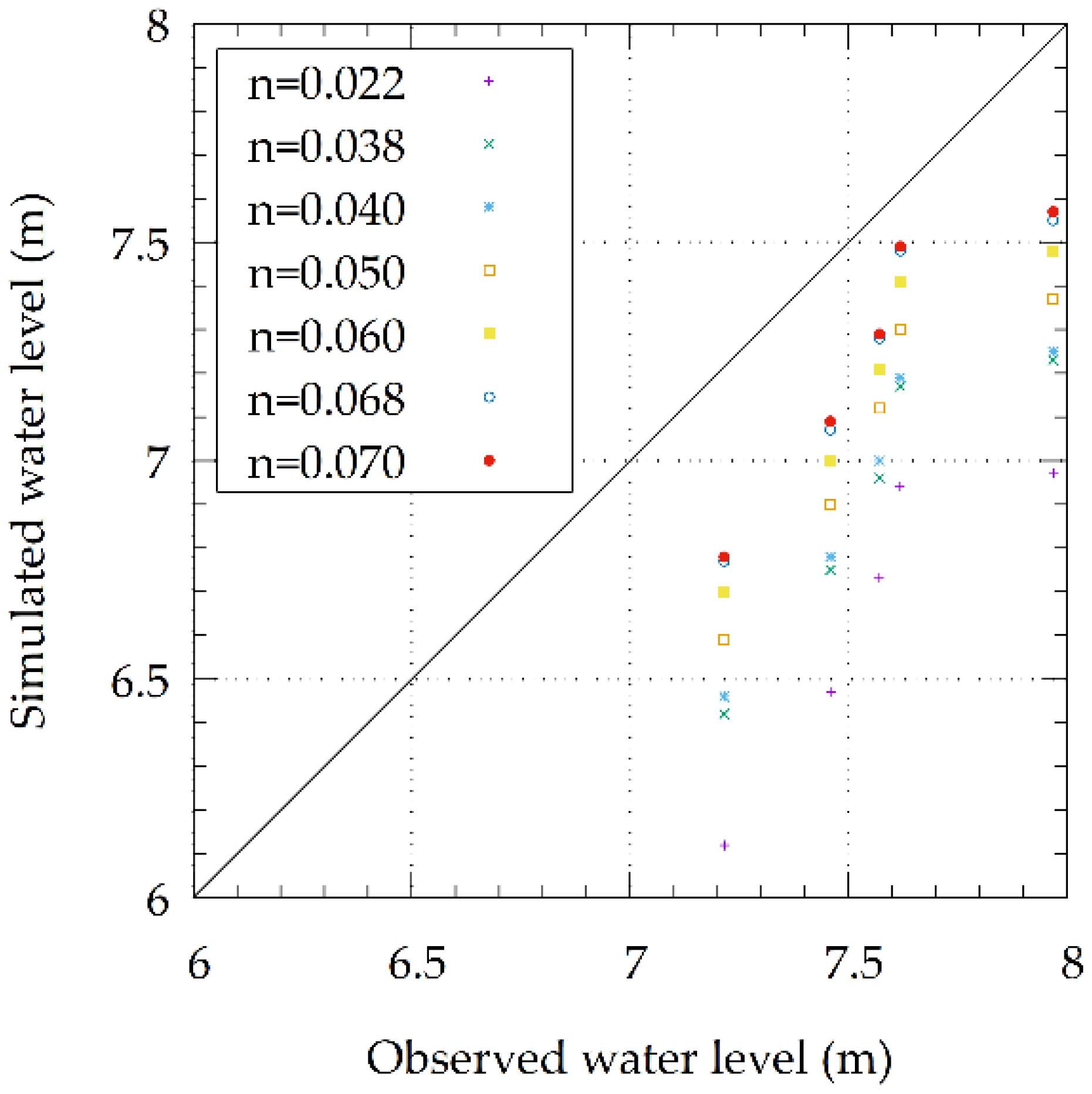
| Manning | RMSE |
|---|---|
| 0.022 | 0.931 |
| 0.038 | 0.671 |
| 0.040 | 0.641 |
| 0.050 | 0.522 |
| 0.060 | 0.421 |
| 0.068 | 0.354 |
| 0.070 | 0.340 |
Publisher’s Note: MDPI stays neutral with regard to jurisdictional claims in published maps and institutional affiliations. |
© 2022 by the authors. Licensee MDPI, Basel, Switzerland. This article is an open access article distributed under the terms and conditions of the Creative Commons Attribution (CC BY) license (https://creativecommons.org/licenses/by/4.0/).
Share and Cite
Araújo Fortes, A.; Hashimoto, M.; Udo, K.; Ichikawa, K.; Sato, S. Dynamic Roughness Modeling of Seasonal Vegetation Effect: Case Study of the Nanakita River. Water 2022, 14, 3649. https://doi.org/10.3390/w14223649
Araújo Fortes A, Hashimoto M, Udo K, Ichikawa K, Sato S. Dynamic Roughness Modeling of Seasonal Vegetation Effect: Case Study of the Nanakita River. Water. 2022; 14(22):3649. https://doi.org/10.3390/w14223649
Chicago/Turabian StyleAraújo Fortes, André, Masakazu Hashimoto, Keiko Udo, Ken Ichikawa, and Shosuke Sato. 2022. "Dynamic Roughness Modeling of Seasonal Vegetation Effect: Case Study of the Nanakita River" Water 14, no. 22: 3649. https://doi.org/10.3390/w14223649