Two-Phase Annular Flow in Vertical Pipes: A Critical Review of Current Research Techniques and Progress

Abstract

Two-phase annular flow in vertical pipes is one of the most common and important flow regimes in fluid mechanics, particularly in the field of building drainage systems where discharges to the vertical pipe are random and the flow is unsteady. With the development of experimental techniques and analytical methods, the understanding of the fundamental mechanism of the annular two-phase flow has been significantly advanced, such as liquid film development, evolution of the disturbance wave, and droplet entrainment mechanism. Despite the hundreds of papers published so far, the mechanism of annular flow remains incompletely understood. Therefore, this paper summarizes the research on two-phase annular flow in vertical pipes mainly in the last two decades. The review is mainly divided into two parts, i.e., the investigation methodologies and the advancement of knowledge. Different experimental techniques and numerical simulations are compared to highlight their advantages and challenges. Advanced underpinning physics of the mechanism is summarized in several groups including the wavy liquid film, droplet behaviour, entrainment and void fraction. Challenges and recommendations are summarized based on the literature cited in this review.

1. Introduction

The building drainage system (BDS) provides a means to safely remove human waste from a building. It consists of vertical ‘stack’ pipes and horizontal ‘branch’ pipes connecting appliances to the vertical stack. The importance of this system in securing public health for occupants has been highlighted recently in the COVID-19 pandemic. Recent work has shown that cross-transmission of pathogens such as SARS and SARS-CoV-2 responsible for the COVID-19 disease, and laboratory surrogate pathogens such as pseudomonas putida (bacterium) and PMMoV (virus), have been shown to travel on airflows inside the BDS which is naturally subject to pressure gradients in the system [1,2,3,4,5]. Understanding two-phase flow in BDS is therefore a public health as well as a fluid mechanics issue.

The flow regime in a drainage system is generated by the unsteady transient flow of a free-falling annular flow, which is a simplified version of a two-phase annular flow with zero or natural airflow and can facilitate the transport of pathogens under certain conditions. An incomplete understanding of the complex two-phase annular flow in vertical pipes limits the extent of current design standards and hence the system quality. Indeed, the vertical annular flow pattern can be found in many important industrial facilities, such as nuclear reactors, refrigeration equipment, heat exchangers and condensers, transportation of oil and natural gas, etc. As the most important two-phase flow regime, annular flow has been widely investigated due to its large involvement in industrial processes and the significant complexity of the flow mechanism.

Professor Hewitt and Professor Azzopardi contributed to the field of annular two-phase flow through their series of studies and significant advancement of knowledge. Hewitt published the fundamental understanding of the annular flow and summarised the literature in 1970, including theoretical models, interfacial waves, and entrained droplets [6]. Azzopardi published a comprehensive review of the literature up to 1997, focused on the droplets in the flow, i.e., entrainment, size, motion, and re-deposition onto the wall film [7]. Berna et al. summarised the research on annular flow with a particular focus on droplet entrainment [8,9]. Relevant review work focusing on the flow maps for two-phase flows in vertical pipe and annuli was reported by Wu et al. in 2017 [10]. However, due to its nature of complexity, it is always challenging to capture detailed and accurate information about the flow at high temporal and spatial resolutions. The incompletely understood annular two-phase flow requires further advancement in experimental techniques, numerical modelling and a better understanding of the mechanism.

Therefore, this paper reviews the investigations on the annular two-phase flow in vertical pipes with a particular focus on the investigation methodologies and advances in understanding the mechanism. Experimental techniques used in previous investigations and numerical modelling are reviewed in the first part of the paper. The challenges of these electrical, optical or mechanical techniques are highlighted at the end of this part. The advanced understanding of the flow characteristics including the wavy liquid film, disturbance waves, droplet behaviours and droplet entrainment is summarized and compared in the second part followed by a conclusion of current challenges and further recommendations.

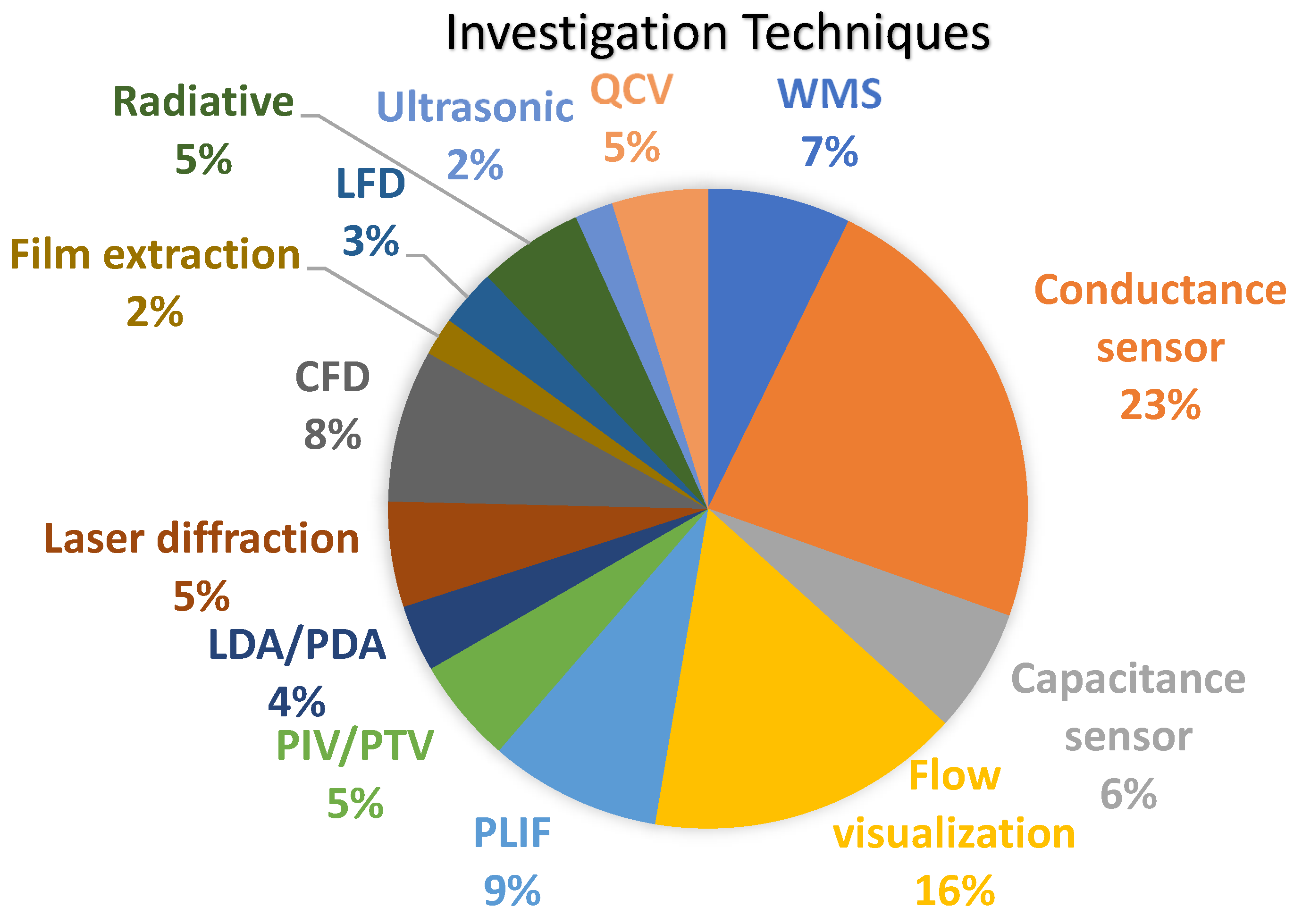
2. Investigation Methodologies

Due to the complexity of the annular flow mechanism, experimental techniques have been widely used to obtain detailed information on the flow properties of the annular two-phase flow. Pressure and temperature profiles can be collected using pressure sensors and temperature sensors. However, it is always challenging to obtain accurate information about the flow, such as fluid/gas velocity, film thickness, droplet entrainment, drop size, drop velocity, void fraction, disturbance waves, etc. Some experimental techniques used to measure the void fraction and flow regime [11], and film thickness [12,13] have been summarized. The following section summarises and evaluates the experimental techniques used in previous research, focusing on the flow regime, annular thin film and entrained droplets, followed by a summary of the numerical investigations in the field.

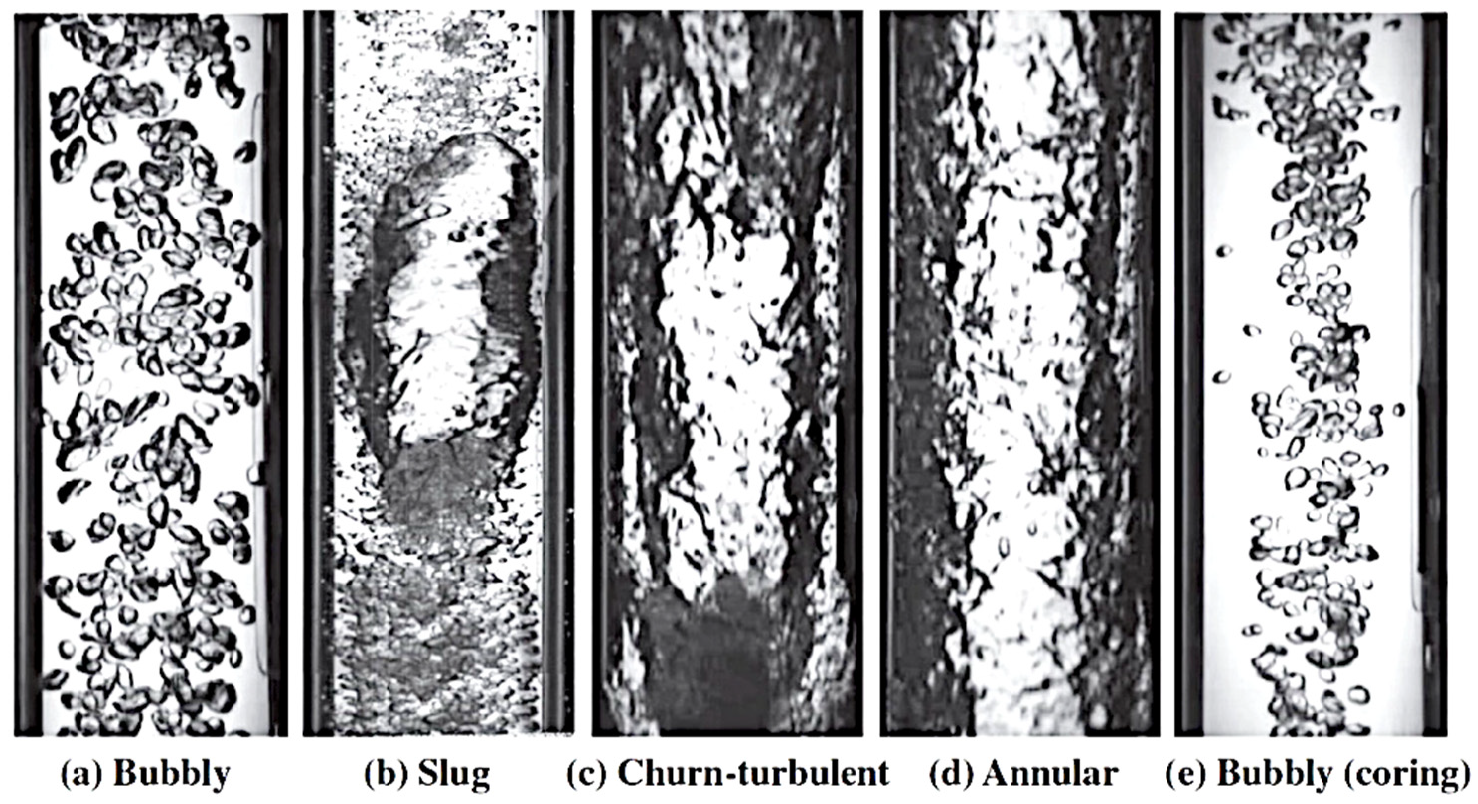
2.1. Visualization and Photography

Due to the development of visual/optical techniques and digital image processing technology, optical methods have shown great advantages in studying gas-liquid two-phase flow, from which qualitative and quantitative results can be obtained. Flow visualization is a useful intuitive method to study flow in transparent pipes, particularly in identifying the flow regime map. Qiao et al. [14] conducted a detailed flow visualization study to characterize the flow regimes in a vertical downward pipe. Flow regime maps for each inlet, including bubbly, slug, churn-turbulent, and annular flow, were developed (as shown in Figure 1). Nimwegen et al. [15,16,17] successfully recorded the visualized flow pattern in a vertical pipe with surfactants, which caused the formation of foam. The videos clearly show the significant impact of the surfactants on flow behaviour. To identify the flow regime, similar visualization results have been observed by different groups of researchers [18,19,20,21,22,23,24,25,26,27,28,29,30,31,32,33,34,35,36,37,38].

Film properties, such as thickness and disturbance wave, can be also captured from the visualization results. Pan et al. [39,40] conducted flow visualization experiments in an air-water two-phase annular flow. High-speed videos of the vertical upward flow were recorded to capture the liquid film properties and disturbance wave data using Matlab code, based on which a prediction model of gas-liquid interfacial shear stress for vertical annular flow was proposed. To minimise the issue of the different refractive indices, a transparent square box was used with water filled inside. Schubring et al. [41], Lin et al. [42,43], Moreira et al. [44] and Barbosa et al. [45] obtained the liquid-film thickness and disturbance-wave characterization from high-speed imaging. Barbosa et al. conducted a series of experiments using a test section with a specially constructed transparent liquid inlet. High-speed video recordings clearly showed the process of wave formation and the wave frequencies and typical velocities were also obtained from the recorded videos.

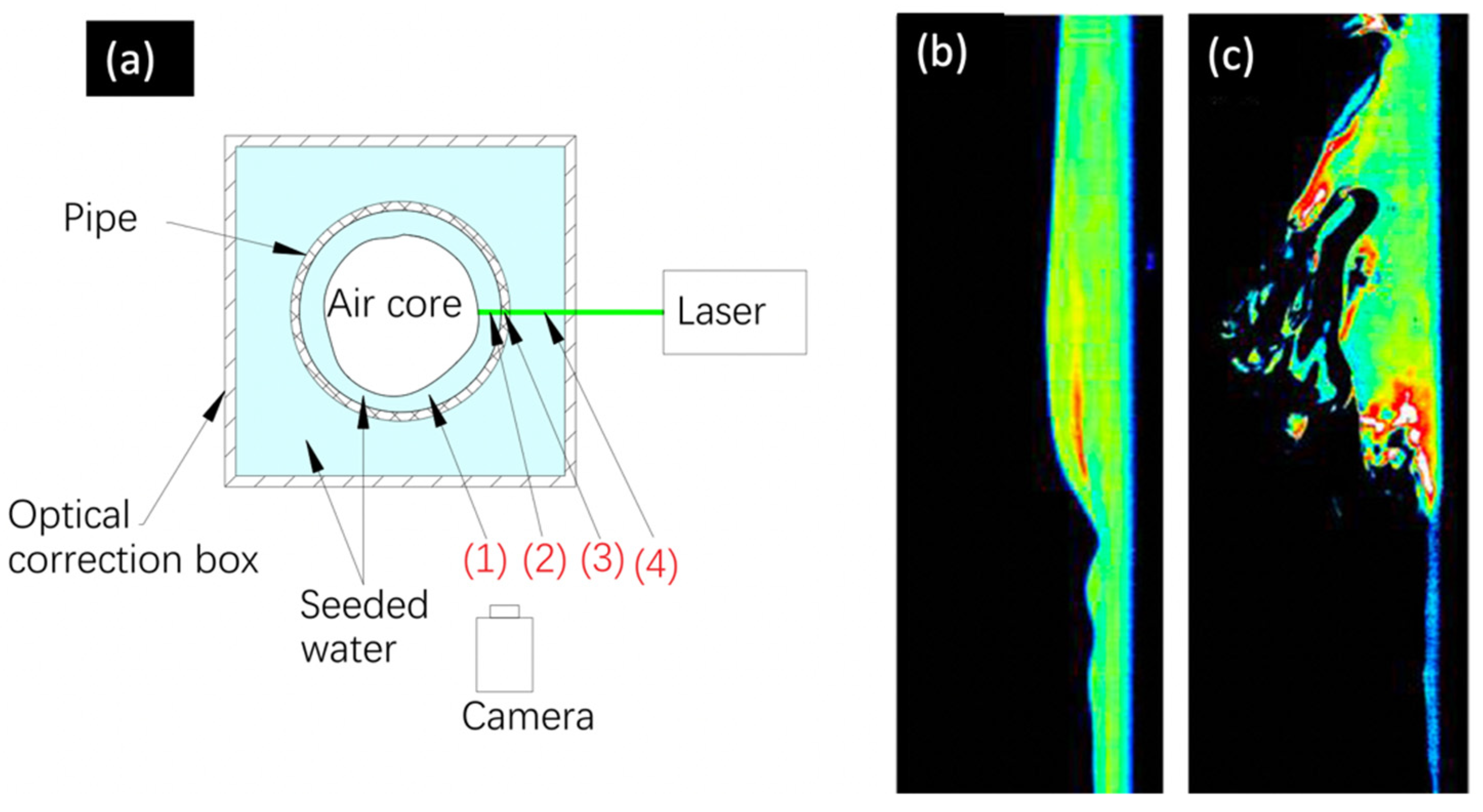
2.2. Laser-Induced Fluorescence (LIF)

To obtain detailed information on the annular film, Laser Induced Fluorescence (LIF) technique has shown broad application prospects due to its high temporal and spatial resolutions. The fluorescence of a certain wavelength can be excited by the laser, which is then captured by a high-speed camera, and the film thickness can be obtained from the recorded images. This enables a measurement of the film thickness and real-time visualization of liquid film flow. A typical experimental setup for a planer laser-induced fluorescence (PLIF) measurement of the liquid film thickness and the visualized liquid film is shown in Figure 2. Häber et al. [46] successfully collected images of the illuminated film and employed a ray-tracing technique to analyse the wavy annular film. They analyzed the errors in the measurement and reported that the uniform film was widened by about 30% due to the deflected fluorescence. Similarly, Eckeveld et al. [47] used a novel implementation of PLIF to measure the film thickness, which had shadows on the laser sheet and appeared as dark lines in the recorded images, preventing strong reflections in the measurements.

Schubring et al. [49,50] also obtained visualization results of the liquid film using PLIF in a vertical annular flow and proposed an improved visualization algorithm for PLIF measurement [51]. Xue et al. [52,53] combined PLIF with high-speed photography to study the liquid film thickness and droplet entrainment. They further [54,55] established a distortion model and proposed a new distortion correction method for the PLIF measurement of the film thickness with a virtual dual-view vision sensor. The method was found capable of measuring circumferential film thickness and distribution characteristics. Vasques et al. [56] used the Brightness Based Laser Induced Fluorescence technique (BBLIF) to study the interfacial wave structure of the liquid film in both upward and downward annular gas-liquid flows. Cherdantsev et al. [13] and Fan et al. [57] also used the BBLIF in the investigation of the co-current downward annular gas-liquid flows as it can be easily resolved in two spatial coordinates and to reconstruct the 3-D shape of the interface wave. Other work using the LIF technique to successfully obtained the film properties in gas-liquid annular flow is seen in [19,48,58,59,60,61,62,63,64].

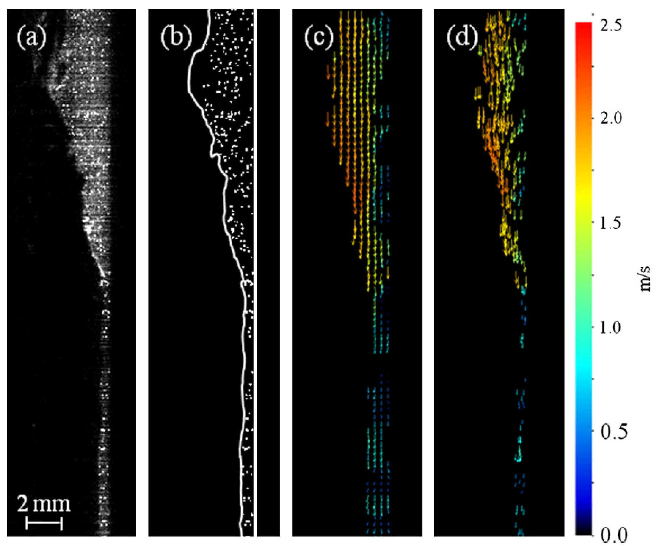
2.3. Particle Image Velocimetry (PIV)

Particle image velocimetry (PIV) and Particle tracking velocimetry (PTV) have been used to obtain the velocity profiles of the liquid film. Illuminated by the laser sheet, the tracer particles can be detected to calculate the velocity vectors. Figure 3 is an example of the liquid film velocity vectors obtained from PIV/PTV measurement by Zadrazil et al. [64,65]. Adomeit and Renz [19] and Ashwood et al. [66] also obtained averaged velocity distribution in a thin annular film using PIV, but the quality of the velocity vector fields was not good. Charogiannis et al. [67] successfully employed simultaneous PIV and LIF measurements in an annular flow to capture the instantaneous velocity vector field and identify the annular film thickness. The main challenges in the application of PIV to obtain the velocity profiles of the liquid film are large velocity gradients in the thin film, strong fluctuation of the free surface, the presence of droplets, and the disturbance waves that can be 10 times the average base film thickness. We have recently conducted PIV measurements of the flow velocity in a gas-liquid annular flow in a vertical pipe. Post-processing of the velocity data and image intensity profile ensures the identification of the interface and hence can provide a statistical understanding of the film thickness and velocity.

2.4. Laser Focus Displacement Meter (LFD)

Annular film properties can be also detected by other techniques, such as laser focus displacement meter, ultrasonic flow meter and near-infrared sensor. Hazuku et al. [68] used a laser focus displacement meter (LFD) to measure the film thickness in an annular flow. Okawa et al. [69] performed film thickness measurements using a laser focus displacement meter, which focuses on a target adopted in automatic focusing. The LFD technique was found capable of accurately measuring film thickness and improving the spatial resolution up to 0.2 µm and time resolution up to 1 kHz. Other similar optical techniques tested in the measurement of the film thickness are the total internal reflection (TIR) method [70,71], the pigment luminance (PLM) method [72] and chromatic confocal imaging (CCI) [73].

2.5. Ultrasonic Flow Meter and Near-Infrared Sensor

Liang et al. [74] measured the film thickness and velocity using ultrasound Doppler velocimetry. Important assumptions include a uniform circumferential liquid film with no waves and no entrained gas. Hence, the measurement accuracy was not as good as other techniques. Wang et al. [75] developed a new ultrasonic echo resonance main frequency (UERMF) measuring system to measure the film thickness and reported an agreement between the conductance probe and the UERMF with an error of less than ±10%. Al-Aufi et al. [76] performed film thickness measurements using ultrasonic pulse-echo techniques and demonstrated the potential of using different signal processing methods. Challenges in the measurement were noticed when the gas-liquid interface experienced large waves. Similarly, near-infrared light sensors have also been used to measure the film thickness based on the different absorption characteristics of gas and liquid [77,78,79,80,81]. However, due to the significant impact of the entrained liquid droplets on the absorption coefficient, light guide pipes were designed and inserted into the annular flow, which ensured the light was only absorbed by the liquid film.

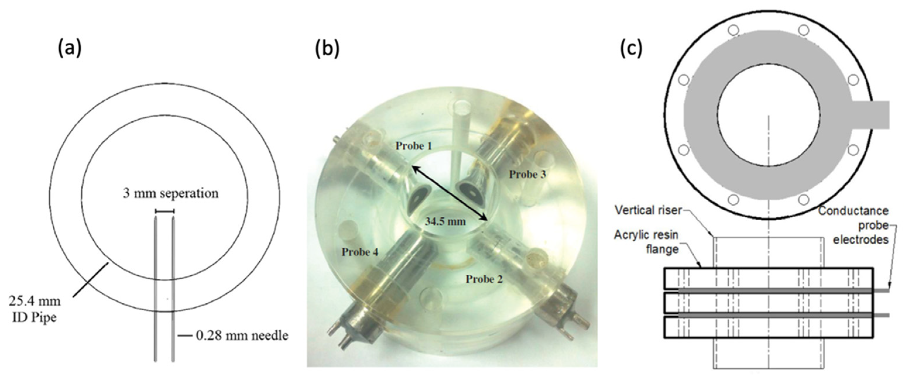
2.6. Conductance Sensor

As one of the widely used sensors, the conductance sensor can measure the film thickness and void fraction in the two-phase annular flow based on the relationship between the fluid fraction and its conductivity. Coney [82] described the theoretical behaviour of flat electrodes wetted by a liquid layer in 1973 and Hewitt [83] reviewed the application of the conductance probe technique up to 1978. Damsohn and Prasser [84] designed a novel flat high-speed liquid film sensor with a high spatial resolution based on the electrical conductance method to measure the thickness of the dynamic liquid films in a two-phase flow, which could be implemented into the annular flow. Some typical conductance probes are shown in Figure 4. The inserted parallel wires probe can capture the local film thickness at the measurement point with a high temporal resolution, while the embedded electrodes are adopted to reduce the disturbance to the film and to measure the average local film thickness.

Wang et al. [85] employed a conductance probe with adjustable insertion depth to measure the film thickness in 2018, and the measurement error was less than 1%. Polansky and Wang [86] applied POD (Proper Orthogonal Decomposition) on a large number of tomograms for the identification of flow patterns in a gas-liquid annular flow. The images were obtained using electrical impedance tomography via a series of electrodes mounted non-intrusively (no induced disturbance to the flow) but invasively (direct contact with the fluid) on the pipe. Measurement of the liquid film thickness by inserting electrodes or parallel wire probes into the pipes is widely used in the field due to its simplicity and low cost [23,24,87,88,89,90,91,92,93,94,95,96,97,98,99,100,101,102,103,104,105,106,107,108,109]. With no induced disturbance to the flow, the embedded electrodes can be grouped as parallel strip electrodes, concentric circle electrodes, circular rod electrodes, ring-shaped electrodes, and so on [12,36,39,40,110,111,112,113,114,115,116,117,118,119,120,121,122,123,124,125,126,127,128].

Figure 4. Some typical conductance probes. (a), Parallel-wire probes [109], 2021 (b), embedded concentric conductance probes [118], 2013 and(c), ring-shaped probes [129], 2019. Figures are adapted with permission from the references, Elsevier.

Figure 4. Some typical conductance probes. (a), Parallel-wire probes [109], 2021 (b), embedded concentric conductance probes [118], 2013 and(c), ring-shaped probes [129], 2019. Figures are adapted with permission from the references, Elsevier.

The conductance probe is capable of measuring the void fraction of the annular flow. Fossa [130] used ring-shaped electrodes and plate electrodes to measure the conductance of the mixtures in pipes and hence to determine the liquid fraction of gas-liquid flow. They further optimised the impedance probes for void fraction measurement in annular, stratified, and dispersed flows [131]. Yang et al. [132] also used conductance probes (3 ring-type impedance meters and 3 arc-type impedance meters) to measure the average void fraction of the two-phase flow.

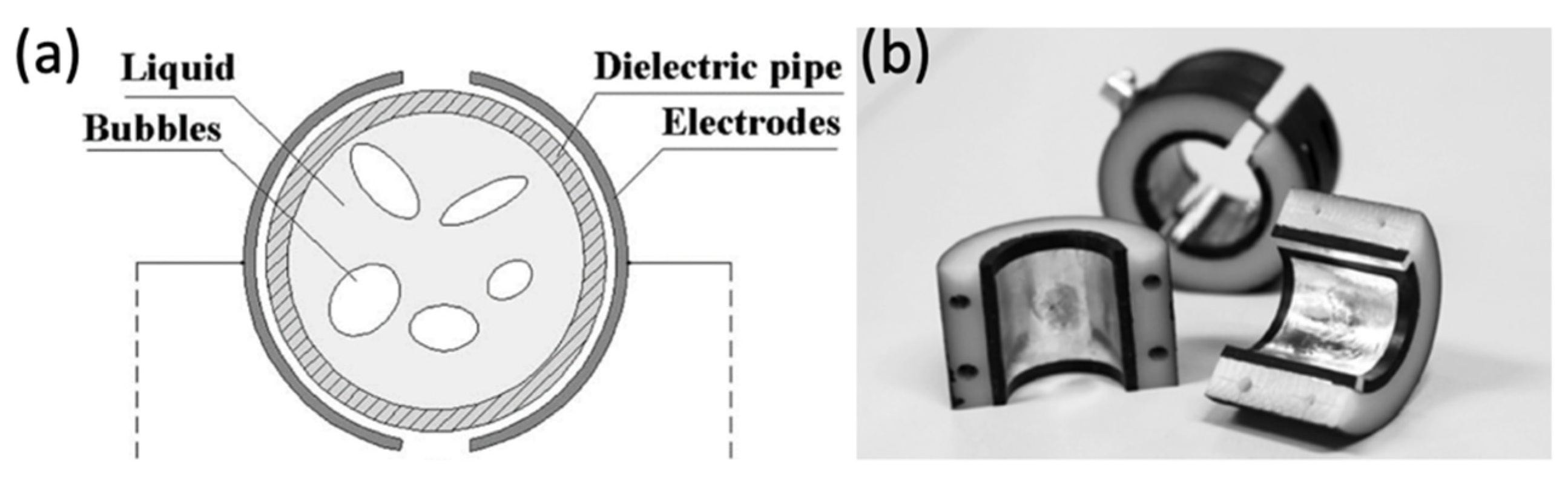
2.7. Capacitance Sensor

In two-phase flow, the permittivity of different fluids is generally different which allows the measurement of the void fraction of the flow components using a capacitance sensor. different types of these capacitance sensors, such as concave [133,134,135], parallel [136], ring [74,137,138,139], and helical [140] sensors, were successfully used in the measurements of the void fraction/gas holdup in the two-phase flows. The selection of this sensor is because it is simple, easy to implement, and relatively low cost. A typical concave capacitance sensor has two concave electrodes mounted on the tube circumference opposite to each other between which the capacitance of the flow is correlated to the local void fraction as shown in Figure 5. A parallel capacitance sensor has several pairs of plates mounted on the outer surface of an insulating pipeline [136]. It can measure the capacitance between all possible combination pairs of the electrodes and then estimate the void fraction based on the image reconstruction algorithm. A ring-type capacitance sensor has two ring electrodes separated in the axial direction of the tube [137] and a helical plate capacitance sensor has two helical electrodes [140].

Atkinson and Huang [141] developed mathematical models for the capacitance sensors used in the measurement of the liquid annulus thickness. Ahmed [139] compared the concave and ring-type capacitance sensors in the void fraction measurement and flow pattern identification in an air/oil two-phase flow experimentally and theoretically. It was reported that the ring-type sensors were more sensitive to the void-fraction signal and had better agreement with the theoretical predictions. Elkow and Rezkallah [140] compared the concave and helical capacitance sensors together with quick-closing valves and a gamma densitometer in the measurement of the void fraction in gas-liquid flows. The fluid temperature was found to have a strong impact on the measured capacitance. Kerpel et al. [142,143] used a concave capacitive void fraction sensor to determine the void fraction and flow regime of a two-phase flow in a small tube. Annular flow, slug flow and intermittent flow were set in the experiment and an alternative calibration technique based on the statistical parameters of the measurement was proposed.

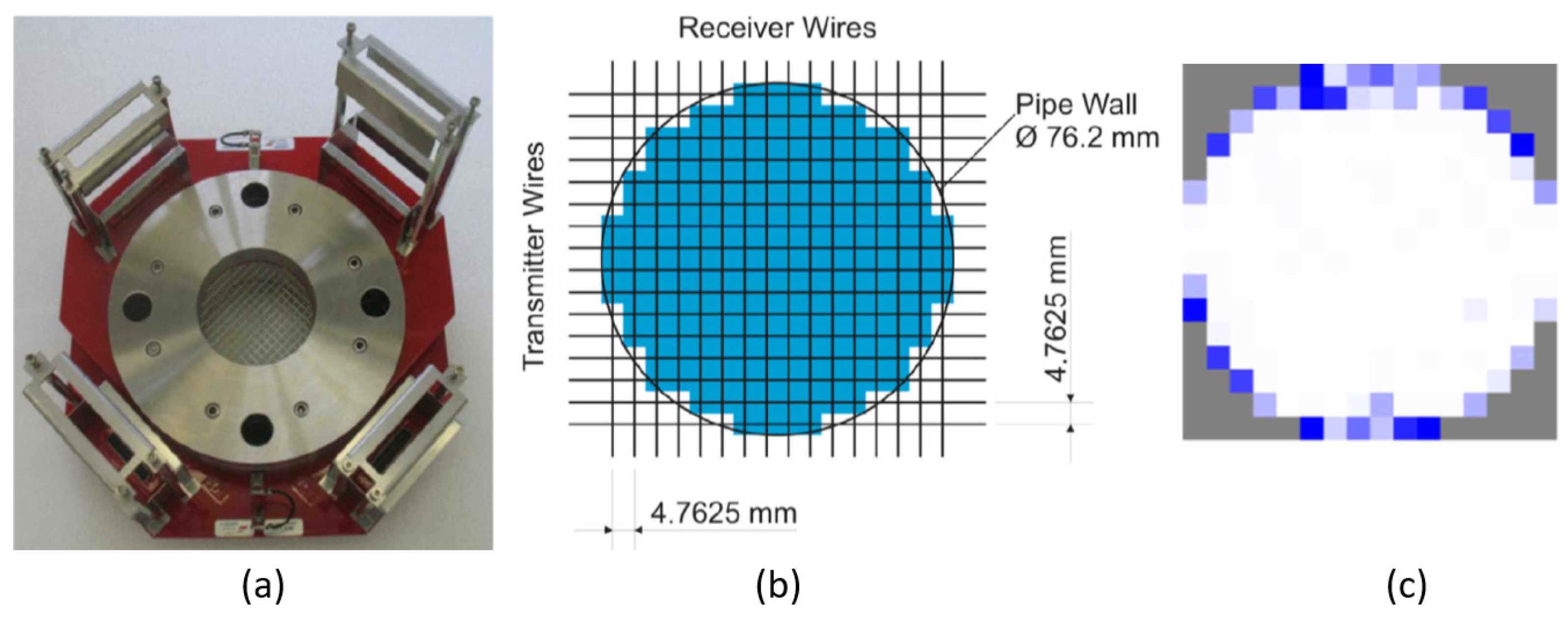
2.8. Wire-Mesh Sensor (WMS)

Phase fraction of two-phase flow (for instance, a droplet in the air core of annular flow or bubbles in bubbly flow) can be also measured using a wire-mess sensor (WMS), as shown in Figure 6, which has two sets of wire electrodes with a small axial displacement between them and being perpendicular to each other. In this way, a matrix-like arrangement of the measuring points (crossing points) is constructed. Based on the different electrical properties of the flow phases, the instantaneous flow conditions at the measurement points can be collected, from which the fractions of the flow phases can be distinguished.

The wire-mesh sensor was first used by Johnson [146] to measure the fraction of water in oil, based on the different conductivities. Prasser et al. [147] further developed an electrode-mesh conductivity sensor, which was the basic form of current WMS, to measure the void fraction distributions of a gas-liquid flow. The wire mesh sensor has been widely used in the measurement of multi-phase flow properties, such as void fraction distribution, flow velocity, bubble size, and film thickness [18,148,149,150,151,152]. Two review articles summarised the application of different types of WMS for the measurement of flow properties in two-phase flows and their associated uncertainties [153,154].

Lucas et al. [155] conducted a comprehensive investigation of the flow properties of an air-water flow in a vertical pipe for a wide range of flow rates (including annular flow). Using the wire-mesh sensor technology, they collected different flow properties, including the gas volume fraction, bubble size, and gas velocity. Vieira et al. [144,145] used a dual WMS with a sampling frequency of 10 kHz to detect the local instantaneous cross-section distribution of the gas core in a vertical pipe. The dual sensor enables simultaneous measurements of the local void fraction at two positions along the flow direction and the flow velocity can be captured from the correlation of the two signals. Silva et al. [156] introduced a novel wire-mesh sensor based on fluid permittivity in a silicone oil bubbly flow. Sensor and measuring electronics were evaluated showing good stability and accuracy in the capacitance measurement.

2.9. Radiative Imaging

As a contactless measurement method, neutron imaging is an attractive option in two-phase flow investigation for the high spatial resolution of the flow structure, such as void fraction and film thickness [157,158,159]. In applications of gamma-densitometry [140,160,161,162,163], the accurate correlation between the loss of radiation intensity and its void fraction provided information on the prevailing flow regime. Banowski et al. [149], Zboray et al. [164] and Misawa et al. [150] used X-ray CT (Computer Tomography) in annular flow and obtained good time series of void fractions.

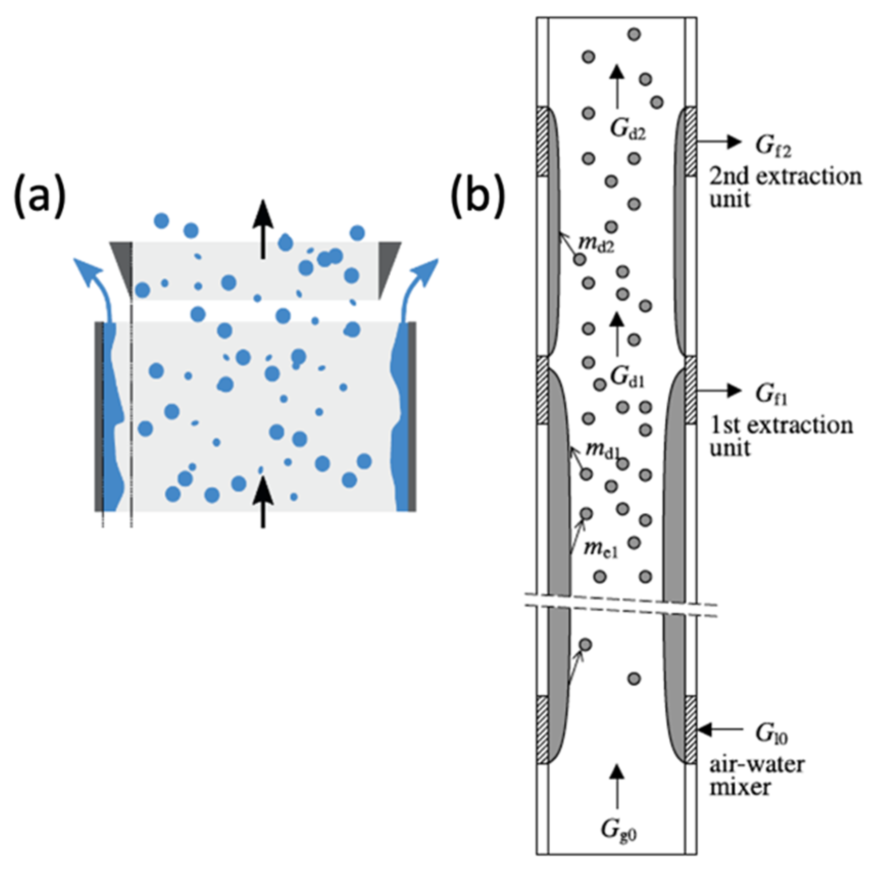
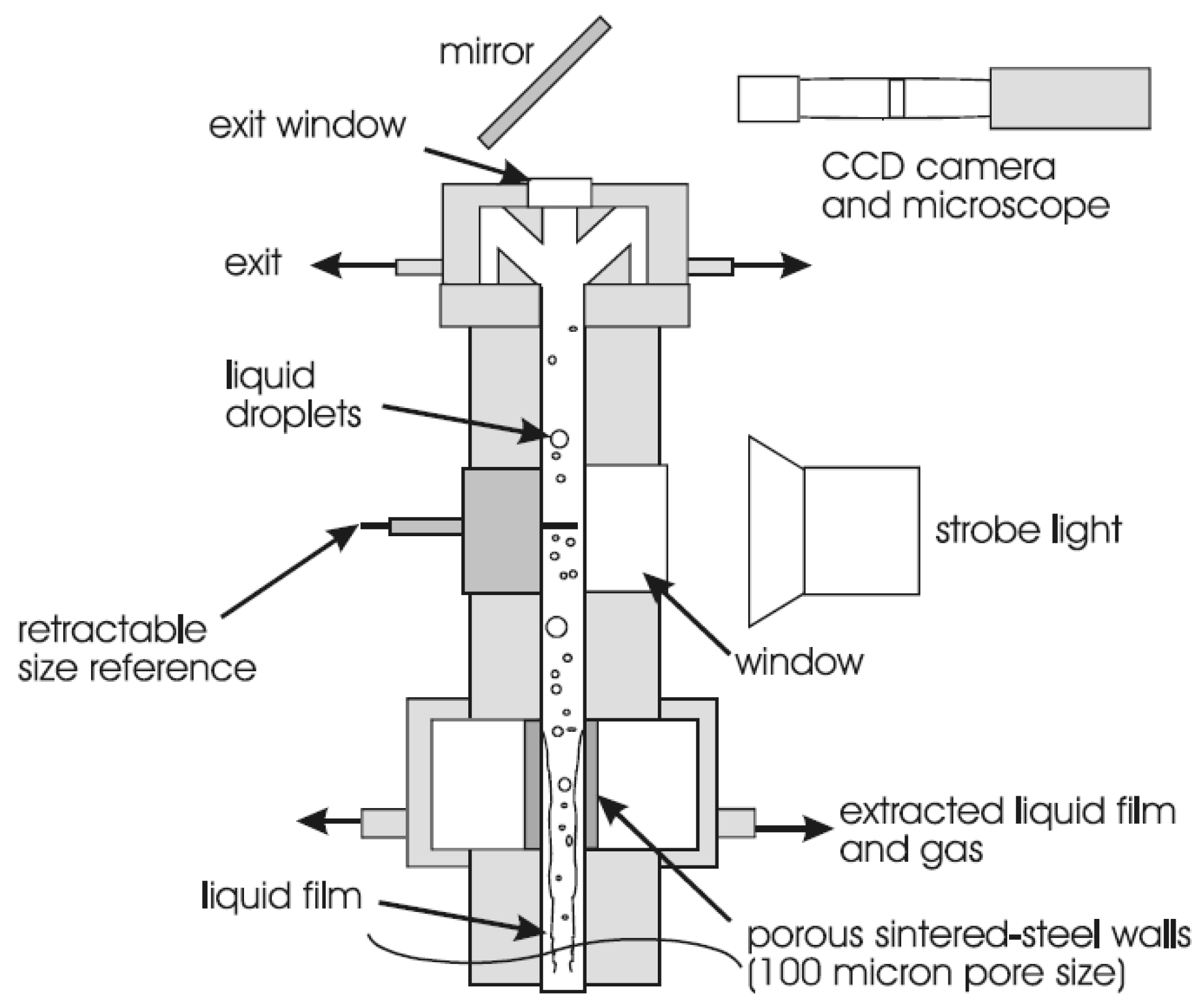
2.10. Film Extraction

The wavy liquid film is always a challenge in investigating the entrained droplets, especially when optical techniques are employed. Therefore, film extraction is generally needed to remove the unsteady optical distortion due to the liquid film and to accurately measure the property of the entrained drops [165]. Figure 7 presents two examples of the film removal configuration in the investigation of the entrained drops in annular flow. The liquid film can be extracted through the porous wall with further purge gas injection at the window or removed from the annular flow through a slightly smaller circular slit. Measurement results of the droplet profiles showed a negligible impact on the film extraction [166].

The extraction of the liquid film was not only required in the visualization study [165] but also needed in laser Doppler anemometry (LDA) [26,167,168] and laser diffraction [99,166,169] measurements. Film extraction can be also used to obtain the void fraction using the flow rate of the separated liquid and gas flow. Bertodano et al. [170], Okawa et al. [171], and Sawant et al. [172] used a film double extraction unit to separate the gas flow and the liquid flow. With single-phase flow meters, the flow rate of the separated liquid/gas flow can be determined which can be used to further calculate the void fraction. However, the droplets entrained in the gas core have to be removed as well, which may otherwise result in non-negligible errors.

Figure 7. (a), Removal of the liquid film by a circular slit with a wedge-shaped edge, adapted with permission from [47], 2018, Elsevier and (b), the extraction of the liquid film by a porous wall for the laser diffraction measurement, adapted with permission from [171], 2005, Elsevier.

Figure 7. (a), Removal of the liquid film by a circular slit with a wedge-shaped edge, adapted with permission from [47], 2018, Elsevier and (b), the extraction of the liquid film by a porous wall for the laser diffraction measurement, adapted with permission from [171], 2005, Elsevier.

2.11. Shadow Photography and Laser Diffraction

With the fluctuating film removed, shadow photography and laser diffraction have shown their capability to measure the droplet size in the gas core. Fore et al. [165] recorded images of the entrain drops in a nitrogen/water annular flow, which had the liquid film extracted through a porous wall (Figure 8). The size of the drops was measured directly from images and statistics analysis provided information on the drop size distribution. When a laser beam passes through a dispersed droplet, the angular variation in the intensity of scattered light is determined by the drop size. In such a way, the distribution of the entrained droplets can be obtained from laser diffraction results. Simmons and Hanratty [166] measured the drop size in air-water annular flow at atmospheric pressure using the laser diffraction technique (Malvern Spraytec R 5008 instrument, Malvern Panalytical Ltd, Malvern, UK). This optical technique has been successfully used by many researchers [47,99,100,169,173,174,175,176,177,178,179] in obtaining the droplet size distribution.

2.12. Laser Doppler Anemometry (LDA)

Another optical technique for the droplet velocity measurement used is the laser Doppler anemometry/phase Doppler anemometry (LDA/PDA) [18,176,179,180]. The velocity can be obtained from the light scattered by the droplets and the Doppler shift, which is related to the velocity component perpendicular to the bisector of the two laser beams. Trabold et al. [161] conducted local measurements in a droplet-laden vapour core in an annular flow, using a gamma densitometer, hot-film anemometer, and LDA. Van’t Westende [167,168] and Zhang et al. [26] used phase Doppler anemometry to measure the size and velocity of the droplets at 11 radial positions of an annular flow.

2.13. Other Mechanical Methods

Barbosa et al. [181] used an isokinetic probe, which was similar to a Pitot tube, to collect the entrained drop and the gas flow of an annular flow, which were then separated for the void fraction measurement. Oliveira et al. [182] achieved accurate measurement of flow rate in gas-liquid flows using a venturi coupled to a void fraction sensor. A quick closing valve (QCV) is another mechanical method to provide an exact void fraction measurement by isolating a section of flow in the conduit and the void fraction can be directly determined [140,183,184,185,186,187,188,189,190,191,192,193,194]. However, it is not a practical method to determine the void fraction for continuous flow as it disrupts the flow. Hurlburt and Hanratty [195] developed an immersion sampling system to measure the droplet diameter in an air-water annular flow. A high-speed shutter apparatus was used to capture the drops in the small cavity filled with high-viscosity oil. The droplet images were processed to obtain drop diameters.

2.14. Numerical Simulation

With the development of computing power, numerical simulation (CFD) has shown its capability to investigate the flow properties of annular two-phase flow. However, due to its complexity, i.e., multi-phase, atomisation, deposition, droplets, bubbles, film, and waves, an accurate and detailed simulation of the annular two-phase flow attracts great interest. A common shortcoming of current CFD models is the treatment method used for the dynamic gas-liquid interface configuration [196]. Because of the challenges in determining the interface dynamics, a simple wave shape or even a smooth gas-liquid interface was used in many of the solution models. Han and Gabriel [196,197,198,199] modelled the gas core flow in a typical annular flow with the simplified flow in the liquid film region. Van der Meulen [18] simulated the droplet behaviour and droplet trajectory in gas-liquid flows in vertical pipes using Star-CD. They also quantified the deposition of the drops by diffusion or direct impaction mechanisms. Xie et al. [200] numerically studied the three-dimensional droplet impacts on a liquid film in a vertical annular flow (Figure 9).

Alipchenkov et al. [201] used a population balance model (PNM) for droplet size distribution, which was based on conservation equations. Liu and Li [202,203] used a CFD-PBM (population balance model) model to investigate the droplet’s size distribution in an annular flow system as well as liquid roll waves directly determined. Van’t Westende [167] performed quasi-1D and 3D large eddy simulation (LES) simulations to compute the pressure gradient and deposition of a dispersed phase in an upward airflow. The PDA measurement results were used in the simulations, mimicking the atomisation process of an actual annular dispersed flow as realistically as possible. Adineh et al. [163] compared the experimental and numerical results of the void fraction inside a vertical pipe with the numerical modelling done using the MCNP (Monte Carlo N-Particle Transport) code. Saxena and Prasser [204] tested different turbulence models to predict the void fraction and capture the liquid film flow properties.

Kishore and Jayanti [205] developed a finite volume method-based model to investigate steady state, 2-D annular flow in a rough-walled duct. It was shown that the simplified model gave reasonable predictions of the flow parameters under equilibrium and non-equilibrium conditions. Kiran et al. [185] tested the VOF (volume of fluid) model and two turbulence models (realizable k-ε and Shear Stress Transport (SST) k-ω models) in the simulation of annular flows at high gas velocity and an average error of 20% was reported. Hassani et al. [206] simulated the two-phase flow using the VOF method and piecewise interface calculation (PLIC) algorithm to track the interface. Fan et al. [57] developed new turbulence damping models to overcome the under-prediction of the turbulence level in the numerical study using the volume of fluid (VOF) method.

It should be noted that some assumptions are generally used in the simulations, such as fully developed and stable annular flow, isothermal flow, no mass exchange between the two phases, uniform distribution of the liquid film, no entrapped gas bubble in the liquid film and uniformly dispersed drops in the gas core. These assumptions can significantly simplify the numerical simulation process but may lead to some non-negligible errors and hence have to be carefully validated.

2.15. Challenges of Current Experimental Techniques

Figure 10 simply summarises the research methodologies used in the investigation of the annular two-phase flow in vertical pipes. The non-invasive and non-intrusive optical measurements, i.e., flow visualization, planar laser-induced fluorescence (PLIF), particle image velocimetry (PIV), particle tracking velocimetry (PTV), the laser Doppler anemometry/phase Doppler anemometry (LDA/PDA), and laser diffraction are getting more attractive due to the main advantage of no disturbance to the flow, high temporal and spatial resolutions, and capability to capture the unsteady flow structure. However, the optical transparency of the pipe or a window that enables the imaging of the flow is essential in the application. Optical distortion of the transparent wall is another limitation that needs to be minimised by a specially designed configuration or corrected in the data post-processing. The main challenge in capturing the wavy film characteristics in annular two-phase flow, particularly the statistical results (for example PIV), is the strong fluctuation of the liquid film thickness. Some other measurement techniques, such as laser focus displacement meter and ultrasonic flow meter, also have limited application due to the complex unsteady flow characteristics in annular two-phase flow.

The electrical sensors, i.e., the wire mesh sensor (WMS), conductance sensor, and capacitance sensor, are still widely used due to their simplicity, reliability, and high temporal resolution. The main limitations of these electrical sensoring technologies are the invasive and intrusive nature of the wires, the requirement of the fluid electrical properties, limited spatial resolution or single-point measurement, and relatively high measurement uncertainty compared to other techniques. As a wire mess sensor needs to be positioned within the pipe, it has a significant impact on the flow properties. It was reported that the WMS caused velocity alteration due to the induced disturbance and a significant pressure drop [147]. It is not applicable to use the WMS in pipe systems which may contain solid components in the flow, such as the drainage system. The successful application of the WMS is also determined by the different electrical properties of the fluids, i.e., conductivity or permittivity, which are significantly different to distinguish the different phases from the electronic signals [154]. The spatial resolution is determined by the number of wires used in each plane. A high resolution of more wires will increase the occupied area and enhance its impact on the flow. Furthermore, the wires must bear the drag forces in the flow, so the larger diameter of the wire, the greater drag force. Both of the two cases are undesirable. Another issue associated with the spatial resolution is the interaction between electrodes, this implies closer electrodes will cause a greater effect and hence lower the measurement quality. The uncertainty of a WMS in void fraction measurement is generally higher than 10% over a wide flow regime [153]. Therefore, in the two-phase annular flow, the applicability of WMS is limited to cases where the film thickness and droplet size are large enough compared to the mesh pitch. The bulk velocity of a WMS is calculated using the assumption that the interfacial velocity is equal to the void velocity. However, this incorrect assumption indicates the inapplicability of this type of measurement [207].

For a conductance probe, the electrical property of the fluid, particularly the temperature, has a significant impact on the measurement result and accuracy. Therefore, it is important to keep the fluid temperature constant during the experiment and to accurately calibrate the probe at the same temperature. Another limitation of the conductance probe is that it only can measure the local property (film thickness or void fraction) at the measurement point. Additionally, the ring type or embedded probe can only measure the average property at the cross-section. While the void fraction or film thickness is generally not available directly from the conductance probe. The accuracy of the conductance probe is generally about 10% [99,100,108].

3. The Wavy Liquid Film

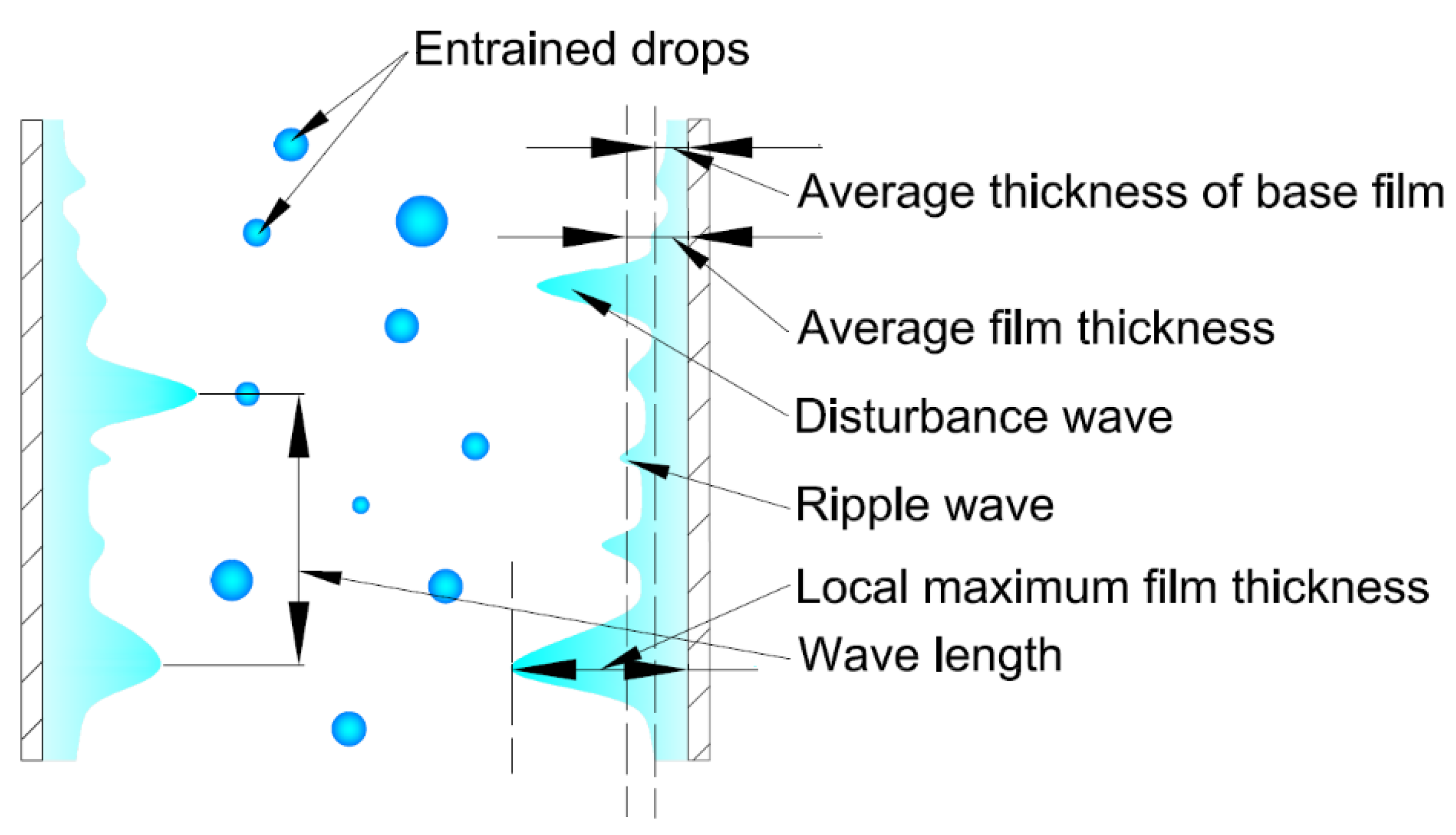
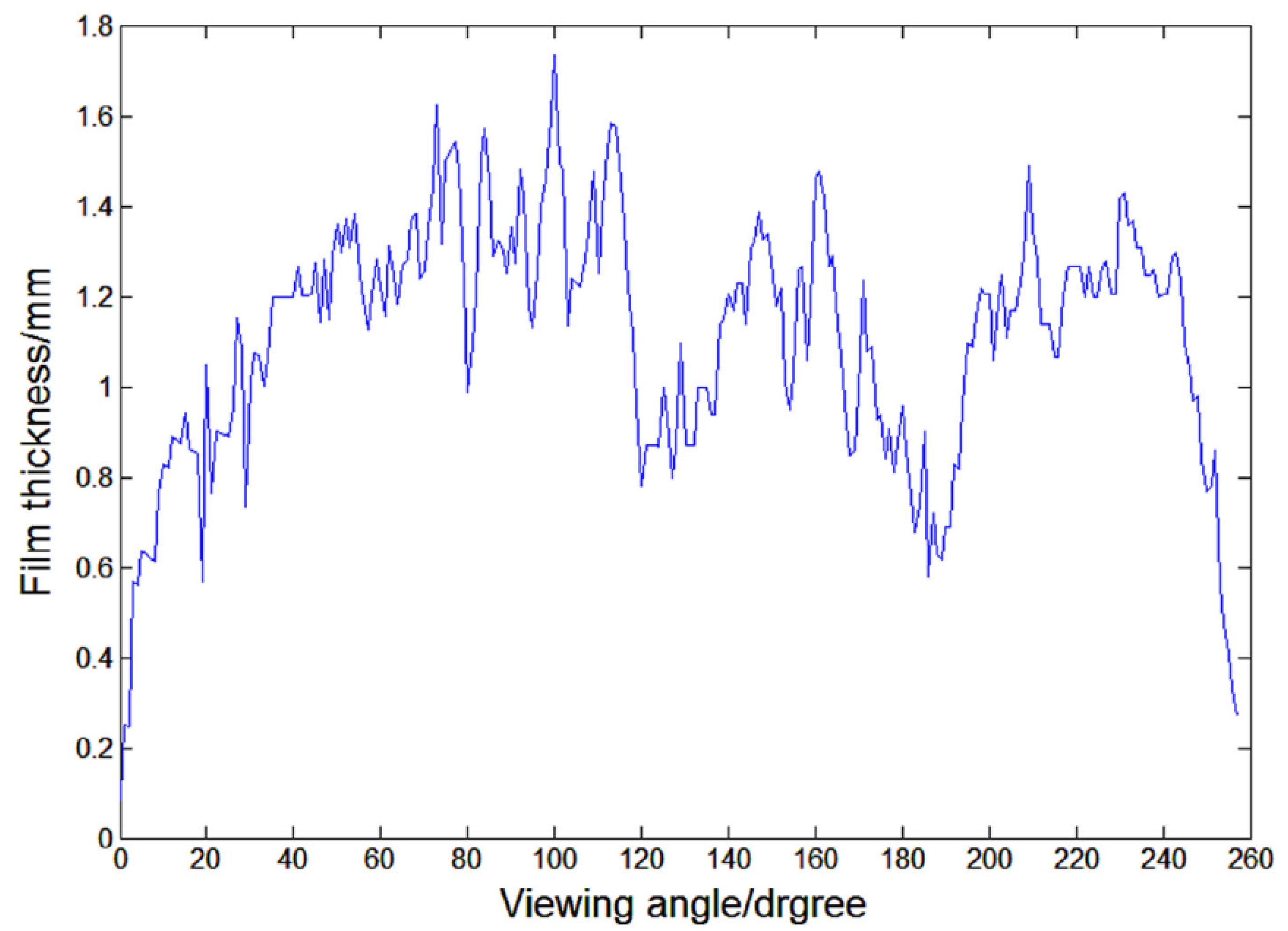
3.1. Fundamental Understanding of the Liquid Film

For an annular two-phase flow in a vertical pipe, the peripheral liquid film generally includes ripple and disturbance waves and acts as a thin wall for the gaseous core flow with entrained drops, as shown in Figure 11. Annular flow gets stable when the fluid has higher effective viscosity (molecular and turbulent viscosity) in the core region and lower viscosity fluid in the annulus [208]. Several definitions are frequently used in the field to describe the flow, such as instantaneous film thickness, the average thickness of base film/substrate, average film thickness, and local maximum thickness. The liquid film thickness is determined by the piping system configuration and the flow conditions such as the liquid flow rate, fluid (gas/liquid) properties, and flow directions. The average liquid film thickness has been well documented in previous research and new understandings of the mechanism have been reported in the recent two decades due to the advanced experimental methods and techniques.

Film thickness distribution captured directly from LIF results [47,49,56,67] (Figure 12) is found similar across a wide range of flow conditions, although the absolute film thickness changes significantly. The average film thickness and the fluctuation of film thickness decreased with gas flow velocity and increased with the liquid flow velocity and the relationship between the average film thickness and the roughness is determined by the liquid and gas flows [50]. Zhao et al. [118] collected high-frequency film thickness data of a gas-liquid annular flow and found the film variation along the axial direction was not significant (within ±10% of average values). The development of the average thickness was only near the inlet, i.e., up to L/D=20 (Re_L = 211) and L/D=25 (Re_L = 603). Prior to becoming fully developed, the film decelerates first to a local maximum thickness and then accelerates again to become thinner.

It is well understood that the film thickness generally decreases with the decrease in the liquid superficial velocity and increases in the gas superficial velocity [18,39,48,99,101,111,112,129,148,209]. The liquid film was reported to have 3-D structures with a large height fluctuation in circumferential and axial directions, and a meandering path between the maximum height around the circumference (Figure 13) [54,55]. This fluctuation is mainly caused by the non-uniform generation of the ripple wave and disturbance waves. This difference in film thickness in circumferential directions was also observed from LIF results [59,60] conductive probe measurements [118,123]. It was found that the average length of the disturbance waves was similar to the pipe diameter and independent of the gas/liquid superficial velocities [123].

A good agreement between the Nusselt’s predictions and experimental velocity profiles was found at low liquid Reynolds number and significant differences between the measured and Nusselt’s predicted profiles were reported in wavy turbulent films (Figure 14), i.e., high Reynolds number [63]. The measured average film thickness data (PLIF) agreed well with previous experimental data and was compared with Nusselt’s theory [48]. The visualization results also proved the existence of recirculation zones in front of disturbance waves [64]. Like the velocity profiles within the wavy film, the film thickness was well-described by the Nusselt flow predictions at low Re_L, while with increasing Re_L, the film thickness was increasingly underpredicted by the theory, but with good agreement with Mudawwar and El-Masri’s semi-empirical turbulence model [210].

Vassallo [211] conducted a near-wall measurement of velocity in the liquid film using a hot-film probe. A modified law of the wall was suggested for annular two-phase flows near the transition regime when the film was thicker. Muñoz-Cobo et al. [125] focused on the effect of the liquid surface tension in vertical annular flow by having different amounts of 1-butanol in the fluid. Reducing the surface tension leads to a reduction in the intermolecular cohesion forces, easier entrainment of the small droplets from the wave peaks and a decrease in the wave amplitude.

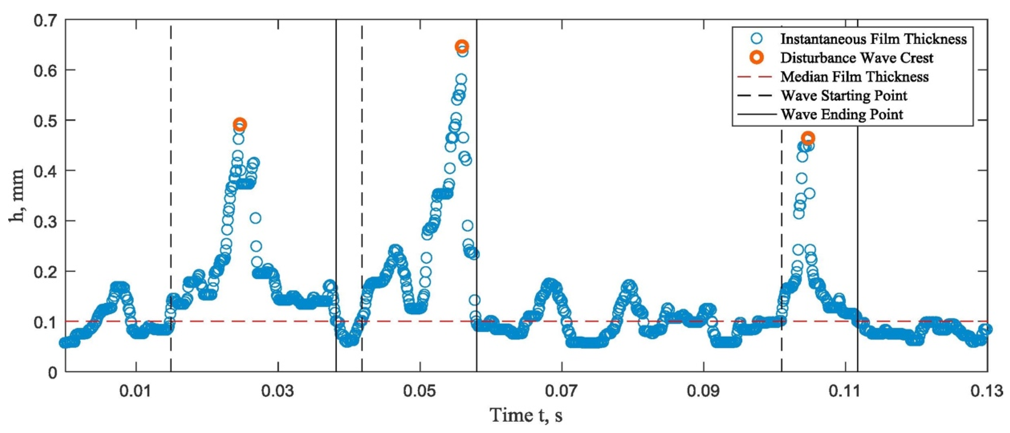
3.2. Disturbance Wave Characteristics

Based on the experimental and numerical results, Fan et al. [57] reported the main progress of wave evolution, i.e., generation and development of initial waves, coalescence of initial disturbance waves into large-scale waves, and acceleration of waves with further stable propagation. They also found that the waves generated slow and fast ripples on their rear slopes and droplet entrainment started from the disruption of fast ripples. The disturbance waves were observed only when the liquid film Reynolds numbers exceeded the critical value [118]. Dao and Balakotaiah [105] investigated the occlusion of falling film in a vertical pipe with glycerine. The experimental results reported a good correlation between the liquid Reynolds number, the Kapitza number, and the Bond number. Han et al. [102] studied the effects of gas flow on the disturbance wave in the annular flow. With a constant liquid flow rate, an increase in the gas mass flow rate resulted in a series of changes in the wave characteristics, i.e., decreased wave spacing and increased wave frequency, slightly decreases in wave base height, peak height, and the mean film thickness. They also reported a much more significant increase in the liquid velocity from the base area to the wavy area with an approximate ratio of 1:14.

Alekseenko et al. [58,59,60,61] reported quantitative studies of the disturbance wave focusing on its spatial and temporal evolution. Three different regions were defined in the liquid film: the crests of disturbance waves, where the fast ripples existed; the back slopes of disturbance waves, where the slow ripples were generated and their properties gradually changed with increasing distance from the crests; and the base film, where the properties of slow ripples had stabilized values. Rapid changes in the film flow parameters, including the thickness, disturbance wave velocity, and frequency, were found within the first 50 tube diameters [111]. The disturbance waves were found to appear and to achieve the stable circumferential distribution at 5–10 pipe diameters from the injection and this coherence gradually strengthened downstream [118].

The identification of the flow pattern and the pressure gradient was determined by the characteristics and behaviours of the interfacial wave [42,43], and its orientation has significant impacts on the flow identification and pressure gradient. Pressure drop in a downward co-current annular flow measured by Hajiloo et al. [212] suggested that at a fixed gas Reynolds number, a large increase in interfacial friction accompanied a decrease in tube diameter and existing correlations were unsuccessful for the present data.

3.3. Correlations of the Film Thickness

Klyuev and Solov’eva [213] developed a mathematical model for the annular flow, which showed the increase in void fraction resulted in decreases in the average film thickness and the average liquid velocity. Belt et al. [209] improved the Wallis correlation by correcting the film roughness, which was assumed as four times the mean film thickness. The new sand-grain roughness was found proportional to the wave height and can be estimated using the roughness density. The transient behaviour model [214] and critical friction factor model [215,216] were developed to estimate the averaged film thicknesses. The calculated results were agreed to within 20% of the experimental measurements. The liquid film at the top was found significantly different from those at the lower axial positions [148], which had a distinctly different slope from the published correlations and theoretical predictions, and hence suggested a potential change in the film structure in large-scale pipes.

Different correlations of the liquid film thickness based on experimental results and theoretical analysis have been proposed so far, which are summarised in

Table 1. Correlations of the average liquid film thickness of annular two-phase flow.

Reference	Correlations of the Liquid Film Thickness
Ishii and Grolmes [217] (1975)	$\delta =0.347R{e}_L^{2/3}\sqrt{\frac{{\rho }_L}{{\tau }_i}}\frac{{\mu }_L}{{\rho }_L}$
Henstock and Hanratty [218] (1976)	$\delta =\frac{6.59F}{{\left(1+1400F\right)}^{0.5}}D$ $F=\frac{1}{\sqrt{2}R{e}_G^{0.4}}\frac{R{e}_L^{0.5}}{R{e}_G^{0.9}}\frac{{\mu }_L{\rho }_G^{0.5}}{{\mu }_G{\rho }_L^{0.5}}$
Tatterson et al. [219] (1977)	$\delta =\frac{6.59F}{{\left(1+1400F\right)}^{0.5}}D$ $F=\frac{\gamma \left(R{e}_L\right)}{R{e}_G^{0.9}}\frac{{\mu }_L{\rho }_G^{0.5}}{{\mu }_G{\rho }_L^{0.5}}$ $\gamma ={\left[{\left(0.707R{e}_L^{0.5}\right)}^{2.5}+{\left(0.0379R{e}_L^{0.9}\right)}^{2.5}\right]}^{0.4}$
Hori et al. [220,221] (1978)	$\delta =0.905R{e}_G^{-1.45}R{e}_L^{0.9}F{r}_G^{0.93}F{r}_L^{-0.68}{\left(\frac{{\mu }_L}{{\mu }_{L,ref}}\right)}^{1.06}D$
Ambrosini et al. [222] (1991)	$\frac{{\rho }_L\delta u^{*}}{{\mu }_L}=\{\begin{array}{c}0.34R{e}_L^{0.6} R{e}_L\le 1000\\ 0.0512R{e}_L^{0,875} R{e}_L>1000 \end{array}, u^{*}=\sqrt{\frac{{\tau }_i}{{\rho }_L}}$
Fukano and Furukawa [94] (1998)	$\delta =0.0594exp\left(-0.34F{r}_G^{0.25}R{e}_L^{0.19}{\chi }^{0.6}\right)D$ $\chi =\frac{j_G{\rho }_G}{j_G{\rho }_G+j_L{\rho }_L}$
Okawa et al. [223] (2002)	$\delta \approx \frac{1}{4}\sqrt{\frac{f_w{\rho }_L}{f_i{\rho }_G}}\frac{\left(1-E\right)j_L}{j_G}D$ $f_i=0.005\left(1+300\frac{\delta }{D}\right)$ $f_w=max\left(\frac{16}{R{e}_L},0.005\right)$
MacGillivray [224] (2004)	$\delta =39\frac{{\mu }_L}{{\rho }_L{j}_L}R{e}_L^{0.2}\frac{1-a}{a}{\left(\frac{{\rho }_G}{{\rho }_L}\right)}^{0.5}$
Hazuku et al. [68] (2008)	${\delta }_{base}{\left(\mathrm{g}/v_L^2\right)}^{1/3}=0.977R{e}_L^{0.143}{\tau }_i^{*-0.117}$ ${\tau }_i^{*}=\frac{{\tau }_i}{{\rho }_L\mathrm{g}}{\left(\frac{g}{v_L^2}\right)}^{1/3}$ ${\tau }_i=\frac{D-2\overline{\delta }}{4}{\left(\frac{dp}{dz}\right)}_{fric}$ ${\tau }_i=f_i{\rho }_G{j}_G^2/2$
Berna et al. [9] (2014)	$\delta =7.156R{e}_G^{-1.07}R{e}_L^{0.48}{\left(\frac{F{r}_G}{F{r}_L}\right)}^{0.24}D$
Pan et al. [39] (2015)	$\delta =2.03R{e}_L^{0.15}R{e}_G^{-0.6}D$
Almabrok et al. [148] (2016)	$\delta =1.4459R{e}_L^{0.3051}{\left(\frac{g}{v_L^2}\right)}^{-\frac{1}{3}}$
Rahman et al. [225] (2017)	$\delta =1.93\times {10}^{-3}R{e}_G^{-0.246}W{e}_G^{-0.161}F{r}_L^{0.15}{\left(\frac{{\dot{m}}_L}{{\dot{m}}_G}\right)}^{0.546}$
Ju et al. [226,227] (2019)	$\delta =0.071tanh\left(14.22W{e}_L^{0.24}W{e}_G^{-0.47}{N}_{{\mu }_f}^{0.21}\right)D$ ${\delta }_{base}=0.04tanh\left(4.31W{e}_L^{0.22}W{e}_G^{-0.44}\right)D$ $N_{\mu f}=\frac{{\mu }_L}{\sqrt{\left({\rho }_L\sigma \sqrt{\frac{\sigma }{g\mathrm{∆}\rho }}\right)}}$ $W{e}_L=\frac{{\rho }_L{j}_L{}^{2}D}{\sigma }, W{e}_G=\frac{{\rho }_G{j}_L{}^{2}D}{\sigma }{\left(\frac{\mathrm{∆}\rho }{{\rho }_G}\right)}^{\raisebox{1ex}{$1$}\!\left/ \!\raisebox{-1ex}{$4$}\right.}$
Rivera et al. [125] (2021)	$\delta =2.35R{e}_G^{-1.415}R{e}_L^{0.414}K{a}^{0.781}D$
Rivera et al. [127] (2022)	$\delta =0.19R{e}_L^{0.54}\left(1-1.29\times {10}^{-5}R{e}_G^{0.93}\right){\left(\frac{v^2}{g}\right)}^{1/3}$
Pan et al. [39]	$\frac{{\delta }_{DW}}{D}=1400{\left(\frac{u_c}{u_L}\right)}^{-\frac{1}{3}}{\left[\frac{({\rho }_L-{\rho }_c)g{\delta }^2}{\sigma }\right]}^{\frac{5}{8}}$
Ju et al. [226]	${\delta }_{DW}=0.24tanh\left(4.22W{e}_L^{0.16}W{e}_G^{-0.46}\right)D$
Y. Rivera, et al. [125]	$\frac{{\delta }_{DW}}{D}=0.554\times {10}^{-3}R{e}_G^{-0.57}R{e}_L^{0.061}K{a}^{1.12}$

.

3.4. The Void Fraction of Annular Two-Phase Flow

The void fraction is the fraction of the gaseous phase to the total volume of the channel, which is generally between 0.65 and 0.98. Godbole et al. [191] conducted a comprehensive literature review of the void fraction correlations and experimental results in the early years of upward two-phase flow. Most area-averaged void fraction had an increasing trend along the axial direction and decreased after a maximum value of around 80–100 diameters downstream [144,145,148]. However, the decrease in void fraction in the vertical downward annular flow was also observed in some conditions which was a result of the kinematic shock phenomenon. Alves et al. [214] developed a three-field two-phase flow model to simulate the transient annular flow in vertical pipes with a slight tendency of underprediction. Smith et al. [103] proposed a one-dimensional interfacial area transport equation (IATE) using measurements of local void fraction, interfacial area concentration, and interface velocity of an upward annular flow in a large pipe. The dependence of mixture density on the void fraction and correlations based on the slip ratio and drift flux model were analysed [228].

Table 2. Correlations for the void fraction (a) of annular two-phase flows.

Reference	Correlations for the Void Fraction
Tandon et al. [229] (1985)	$a=\left\{1-1.928R{e}_L^{-0.315}{\left[F\left(X_{tt}\right)\right]}^{-1}+0.9293R{e}_L^{-0.63}{\left[F\left(X_{tt}\right)\right]}^{-2}\right\} 50<R{e}_L<1125$ $a=\left\{1-0.38R{e}_L^{-0.088}{\left[F\left(X_{tt}\right)\right]}^{-1}+0.0361R{e}_L^{-0.176}{\left[F\left(X_{tt}\right)\right]}^{-2}\right\} R{e}_L>1125$ $F\left(X_{tt}\right)=0.15\left[X_{tt}^{-1}+2.85X_{tt}^{-0.476}\right]$ $X_{tt}={\left(\frac{{\mu }_L}{{\mu }_G}\right)}^{0.1}{\left(\frac{1-x}{x}\right)}^{0.9}{\left(\frac{{\rho }_G}{{\rho }_L}\right)}^{0.5}$
Usui and Sato [93] (1989)	${\left(1-a\right)}^{23/7}-2C_{w}F{r}_L^2\left[1\pm \frac{C_i}{C_w}\mathrm{·}\frac{{\left(1-a\right)}^{16/7}}{a^{5/2}}\mathrm{·}\frac{{\rho }_G}{{\rho }_L}{\left(\frac{j_G}{j_L}\right)}^2\right]=0$ Free falling film, $a=1-{\left(2C_{w}F{r}_L^2\right)}^{7/23}$
Cioncolini and Thome [230] (2012)	$a=\frac{h{x}^n}{1+\left(h-1\right)x^n}$ $(0<x<1, {10}^{-3}<\frac{{\rho }_G}{{\rho }_L}<1, 0.7<\epsilon <1)$ $h=-2.129+3.129{\left(\frac{{\rho }_G}{{\rho }_L}\right)}^{-0.2186}$ $n=0.3487+0.6513{\left(\frac{{\rho }_G}{{\rho }_L}\right)}^{0.515}$
Kumar et al. [194] (2017)	${\left(1-a\right)}^{23/7}-2C_{w}F{r}_L^2\left[1\pm \frac{C_i}{C_w}\mathrm{·}\frac{{\left(1-a\right)}^{16/7}}{a^{5/2}}\mathrm{·}\frac{{\rho }_c}{{\rho }_L}{\left(\frac{j_G}{j_L}\right)}^2\right]=0$ Free falling film, $a=1-{\left(2C_{w}F{r}_L^2\right)}^{1/3}$

summarized the correlations for the void fraction (a) annular two-phase flows.

4. The Entrained Droplets in the Central Gas Core

4.1. Droplet Behaviour

The surface instability is the reason for droplet formation and its entrainments. In an annular two-phase flow, the top part of the disturbance wave is undercut and forms an open-ended bubble with a filament rim. This bag breaks into many small droplets and the rim’s break-up results in a smaller number of larger drops. Some of the droplets can deposit onto the liquid film and hence leads to a decrease in the entrainment. The droplet entrainment was well discussed and summarised by Prof. Azzopardi [7] and supported by recent experimental results as shown in Figure 15 [48]. Kumar et al. [231] numerically observed wave-like protrusion in an orifice, a bag-like break-up in undercutting, and ligament fragmentation that results in dislodge of droplets from the film (Figure 15g). The entrained droplet generally moves with the gas core, with its distribution of size varying in time and space. Tube diameter has been found to have little influence on the sizes of drops [169]. In contrast, the drop size was determined by the liquid flow rate and viscosity, increasing with increases in both [180,232]. The models used to describe the onset of entrained liquid fraction were reported invalid with high viscosity liquid [233] and the droplets in the early stage could be larger than any stable droplet in convection pipe flow [234].

Okawa et al. [171] conducted a series of measurements focusing on the droplet entrainment and deposition of an annular two-phase flow in a small vertical tube. The entrainment rate had a good correlation with the dimensionless number denoting the interfacial shear force and surface tension, while the deposition rate was determined by the droplet concentration in the gas core. It is also reported that at low drop concentrations, the deposition rate varied linearly but was not sensitive at high concentrations [232]. In another work [177], the droplet deposition rate was determined by the deposition constant and the drop velocity fluctuations. Xie et al. [200] studied the three-dimensional droplet deposition process and reported detailed complex interfacial structures during droplet impact.

Zhang et al. [32] measured the size and velocity of the droplets and reported that the ligament break-up of waves produced a large number of drops with high velocity and sphericity. The droplets had a continuous size distribution and the size increased slightly during the accelerated migration in the gaseous core. The droplets experienced axial acceleration and radial deceleration during the radial migration, but the overall distribution of droplet size and velocity remained unchanged. Starting with a small number, the proportion of relatively large drops gradually increased and their impacts on the total momentum could not be neglected. Alamu and Azzopardi [99,100] reported that both wave and droplet dominant frequency increased with an increase in the superficial velocities of both gas and liquid and drops became more elastic as liquid superficial velocity increased.

Trabold and Kumar [161,235] found the vapour turbulence was enhanced by the droplets over the range of drop size and concentration. However, improvement of the experimental technique and reduction in the measurement uncertainties were highly recommended as the uncertainty could be up to 25%. To further reconcile the droplet diameters obtained by various researchers, a definitive study is also highly recommended [7]. Liu and Li [202] showed it was possible to numerically predict the drop size distribution in annular two-phase flow using coalescence and breakup kernels. However, the only good prediction of the large droplets implied that it was necessary to develop a more accurate model. Based on Kataoka’s correlation [236], Fore et al. [165] proposed a prediction of the drop size, which is given in

Table 3. Predictions of the drop size in an annular flow.

Reference	Prediction of the Droplet Size
Kocamustafaogullari et al. [234] (1994)	$\frac{d_{32}}{D}=0.64C_W^{-4/15}W{e}_m^{-3/5}{\left(\frac{R{e}_G^4}{R{e}_L}\right)}^{4/15}{\left(\frac{{\rho }_G}{{\rho }_L}\right)}^{4/15}{\left(\frac{{\mu }_G}{{\mu }_L}\right)}^{4/15}$$C_w=1/35.34N_{\mu }^{\frac{4}{5}} \left(N_{\mu }\le 1/15\right)$ $C_w=0.25 (N_{\mu }>1/15)$
Azzopardi [7] (1997)	$\frac{d_{32}}{D}=1.91R{e}_G^{0.1}W{e}_G^{-0.6}{\left(\frac{{\rho }_G}{{\rho }_L}\right)}^{0.6}+0.4\frac{E{j}_L}{j_G}$
Fore et al. [165] (2002)	$\frac{d_v}{D}=0.028W{e}_G^{-1}R{e}_L^{-1/6}R{e}_G^{2/3}{\left(\frac{{\rho }_G}{{\rho }_L}\right)}^{-1/3}{\left(\frac{{\mu }_G}{{\mu }_L}\right)}^{2/3}$
Azzopardi [237] (2006)	$d_{32}=\left[0.069j_G+0.0187{\left(\frac{{\rho }_L{j}_L}{{\rho }_G{j}_G}\right)}^2\right]\frac{\sigma }{{\rho }_G{j}_G}$
Berna et al. [8] (2015)	$\frac{d_v}{D}=0.11W{e}_G^{-0.68}R{e}_G^{0.33}R{e}_L^{0.11}{\left(\frac{{\rho }_G}{{\rho }_L}\right)}^{0.31}$
Wang et al. [180] (2020)	$\frac{d_{32}}{D}=0.022W{e}_G^{-0.545}W{e}_L^{0.214}R{e}_L^{-0.249}R{e}_G^{0.439}{\left(\frac{{\rho }_G}{{\rho }_L}\right)}^{0.117}$

as well as other recently proposed correlations.

4.2. Correlation of Droplet Entrainment

Droplet entrainment fraction (E) is defined as the ratio of the entrained liquid drop mass flow rate divided by the total liquid mass flow rate and the entrainment rate (ε) is defined as the entrained drop mass rate per unit area of the gas-liquid interface. It has been shown that most of the predictions developed were very restricted in a wide variety of flow conditions. And there has not been a general correlation for the entrainment fraction so far [238]. The correlations of the droplet entrainment rate and entrainment fraction of the annular two-phase flow reported recently are summarised in

Table 4. Correlations for the droplet entrainment rate in annular flows.

Reference	Correlations of the Droplet Entrainment Rate
Bertodano et al. [170] (1997)	$\frac{\epsilon D}{{\mu }_L}=k{\left[W{e}_G{\left(\frac{\mathrm{∆}\rho }{{\rho }_G}\right)}^{1/2}\left(R{e}_{Lf}-R{e}_{Lfc}\right)\right]}^{0.925}{\left(\frac{{\mu }_G}{{\mu }_L}\right)}^{0.26}$ $R{e}_{Lf}=R{e}_L\left(1-E\right)$
Kataoka et al. [239] (2000)	$\frac{\epsilon D}{{\mu }_L}=6.6\times {10}^{-7}R{e}_L^{0.74}R{e}_{Lf}^{0.185}W{e}^{0.925}{\left(\frac{{\mu }_G}{{\mu }_L}\right)}^{0.26}$
Bertodano et al. [240] (2001)	$\frac{\epsilon D}{{\mu }_L}=\frac{3.8\times {10}^{-6}\sigma }{4}\left(R{e}_{Lf}-R{e}_{Lfc}\right)W{e}_G{\left(\frac{\mathrm{∆}\rho }{{\rho }_G}\right)}^{1/2}$
Okawa and Kataoka [241] (2005)	$\epsilon ={\rho }_{L}min\left(0.0038{\pi }_{e1},0.0012{\pi }_{e1}^{0.5}\right)$ ${\pi }_{e1}=\frac{f_i{\rho }_G\left(j_G^2-j_{Gc}^2\right)\delta }{\sigma }$
Ryu and Park [242] (2011)	$\epsilon ={\rho }_L{V}_e\frac{u_G-u_{DW}}{4h{\lambda }^2\sqrt{a}}$
Liu and Bai [243] (2017)	$\epsilon =4.347\times {10}^{-6}{\rho }_{L}R{e}_L^{0.584}{\left(\frac{{\rho }_L}{{\rho }_G}\right)}^{0.0561}{\left(\frac{{\tau }_i\delta }{\sigma }\right)}^{0.391}{\left(\frac{D}{\sqrt{\sigma /g\mathrm{∆}\rho }}\right)}^{-0.291}$ ${\tau }_i=f_i{\rho }_G{j}_G^2/2$
Wang et al. [244] (2020)	$\epsilon ={\epsilon }_{max}\times tanh\left(3.56\times {10}^{-6}R{e}_{la}^{0.47}W{e}^{1.15}\right)$ $\frac{{\epsilon }_{max}\sqrt{\sigma /g\mathrm{∆}\rho }}{{\mu }_L}=\{\begin{array}{c}0.00515R{e}_{la}^{0.69} \left(R{e}_{la}\le 800\right)\\ 0.521 (R{e}_{la}>800)\end{array}$ $R{e}_{la}=\frac{{\rho }_L{j}_L\sqrt{\sigma /g\mathrm{∆}\rho }}{{\mu }_L}$

and

Table 5. Correlations for entrainment fraction in annular two-phase flows.

Reference	Correlations for the Entrainment Fraction
Oliemans et al. [245] (1986)	$\frac{E}{1-E}={10}^{-0.25}{\rho }_L^{1.08}{\rho }_G^{0.18}{\mu }_L^{0.27}{\mu }_G^{0.28}{\sigma }^{1.80}{D}^{1.72}{j}_L^{0.7}{j}_G^{1.44}{g}^{0.46}$
Ishii and Mishima [246] (1989)	$E=tanh\left(7.25\times {10}^{-7}W{e}_G^{1.25}R{e}_L^{0.25}\right)$
Utsono and Kaminanga [247] (1998)	$E=tanh\left(0.16R{e}_L^{0.16}W{e}_G^{0.08}-1.2\right)$
Petalas and Aziz [248] (2000)	$\frac{E}{1-E}=0.735{\left(\frac{{\mu }_L^2{j}_G^2{\rho }_G}{{\sigma }^2{\rho }_L}\right)}^{0.074}{\left(\frac{j_L}{j_G}\right)}^{0.2}$
Barbosa et al. [181] (2002)	$E=0.95+342.55\sqrt{\frac{{\rho }_L{\dot{m}}_L}{{\rho }_G{\dot{m}}_G}}{D}^2$
Pan and Hanratty [249] (2002)	$\frac{E/E_M}{1-E/E_M}=6\times {10}^{-5}{\left(u_G-u_{Gc}\right)}^2\sqrt{{\rho }_G{\rho }_L}D/\sigma$ $E_M=1-\frac{{\dot{m}}_{lfc}}{{\dot{m}}_l}$
Sawant et al. [250] (2008)	$E=\left(1-\frac{250\ln R{e}_L-1265}{R{e}_L}\right)tanh\left(2.31\times {10}^{-4}R{e}_L^{-0.35}W{e}_G^{1.25}\right)$
Sawant et al. [172] (2009)	$E=\left[1-\frac{13N_{\mu f}^{-0.5}+0.3{\left(R{e}_L-13N_{\mu f}^{-0.5}\right)}^{0.95}}{R{e}_L}\right]tanh\left(2.31\times {10}^{-4}R{e}_L^{-0.35}W{e}_G^{1.25}\right)$ $N_{\mu f}=\frac{{\mu }_L}{\sqrt{\left({\rho }_L\sigma \sqrt{\frac{\sigma }{g\mathrm{∆}\rho }}\right)}}$
Cioncolini and Thome [251] (2010)	$E={\left(1+13.18W{e}_c^{-0.655}\right)}^{-10.77}$ $W{e}_c=\frac{{\rho }_c{u}_c^2{D}_c}{\sigma }$
Cioncolini and Thome [252] (2012)	$E={\left(1+279.6W{e}_c^{-0.8395}\right)}^{-2.209}$ $W{e}_c=\frac{{\rho }_c{j}_G^2{D}_c}{\sigma }$
Berna et al. [8] (2015)	$\frac{E}{1-E}=5.51\times {10}^{-7}W{e}_G^{2.68}R{e}_G^{-2.62}R{e}_L^{0.34}{\left(\frac{{\rho }_G}{{\rho }_L}\right)}^{-0.37}{\left(\frac{{\mu }_G}{{\mu }_L}\right)}^{-3.71}{C}_w^{4.24}$ $C_w=\{\begin{array}{c}0.028N_{\mu }^{-0.8} \left(N_{\mu }\le 1/15\right)\\ 0.25 (N_{\mu }>1/15)\end{array}$
Aliyu et al. [152] (2017)	$E=\{\begin{array}{c}\frac{1\times {10}^{-2}W{e}^{0.33}R{e}_L^{0.27}}{1+1\times {10}^{-2}W{e}^{0.33}R{e}_L^{0.27}}\\ \frac{1.25\times {10}^{-3}W{e}^{0.15}R{e}_G^{0.2}R{e}_L^{0.23}}{1+1.25\times {10}^{-3}W{e}^{0.15}R{e}_G^{0.2}R{e}_L^{0.23}}\end{array} \begin{array}{c}(j_G>40 m/s)\\ (j_G\ll 40 m/s)\end{array}$
Zhang et al. [253] (2020)	$E\approx 0.075\frac{D{\rho }_L{\rho }_G^2{\delta }^2{u}_{*}^8}{j_L{\mu }_G^{\frac{2}{3}}{\sigma }^{\frac{7}{3}}{u}_G^{\frac{5}{3}}}{\left(\frac{\delta }{D}\right)}^{\frac{1}{3}}$

in this section. In our recent work, the droplet entrainment of an annular two-phase flow in a vertical pipe was obtained using the film extraction technique. The entrainment fraction is plotted against various flow rates at different heights, which shows the developing process of the entrained drops to a steady state. The impact of the ventilation on the flow behaviour of the annular flow, i.e., with or without the central gas flow, is examined in form of entrained droplets, which shows a negligible difference in entrainment fraction. These results will be published soon with annular velocity and thickness profiles.

5. Conclusions and Recommendations

Annular two-phase flows in vertical pipes widely exist in many industrial applications, which have been investigated since the early years of fluid mechanics. This is also the case with annular flow in building drainage systems. Aiming to provide a general understanding of the current state of understanding on the topic, this work provides a review of the research in the most recent two decays, with a particular focus on the experimental techniques and advanced understanding of the mechanism underpinning annular flow.

Experimental techniques used in the field are summarised and their advantages and limitations are discussed in Section 2.15. These challenges, such as distortion of the transparent wall in optical measurements, strong fluctuation of the liquid film, and disturbance induced by the inserted probes, further imply the need for new or improved techniques to capture the detailed flow properties of annular two-phase flow, particular with these characteristics, high accuracy, simplicity and suitability for wide industrial applications. Lots of analytical expressions and empirical correlations of the liquid film thickness, disturbance wave property, droplet entrainment, drop size and void fraction has been proposed. on the other hand, this indicates the lack of a well-accepted model that can accurately predict the flow parameters in a wide range of flow and pipe conditions.

With the development of experimental techniques and computing capacity in the last two decays, the understanding of the complex two-phase annular flow in vertical pipes has been significantly advanced, for instance, the clear capture of the liquid film fluctuation and droplet generation. It is not surprising to note that all previous investigations are focused on steady flow conditions, including the transient flow region near the inlet of a stable annular flow, which is more frequently used, easier to measure and simpler to model. However, unsteady annular two-phase flow, which can be also seen in some cases and is always found in a building drainage system, has not been widely investigated and is not well understood. The current understanding of unstable annular flow is generally derived from the steady-state annular flow. Therefore, investigation of unsteady annular flow and transient region of a stable flow is recommended with particular focus on the wavy liquid film, gas core and entrained drops. It would therefore be reasonable to suggest that building drainage codes (particularly for tall buildings) should incorporate elements of this new understanding.

It should be also emphasized that the gas flow in the central core region is not an essential requirement for annular two-phase flow in vertical pipes. When gas velocity in the central region is set to zero, or the ventilation pipe is closed in a free-falling flow, similar flow features should be observed in a vertical pipe, such as film development, disturbance wave, and droplet entrainment. But many previous theoretical or empirical models have gas flow as one of the dominating mechanisms and non-negligible gas superficial velocity in the formulas. These models have obvious limitations in predicting annular flow with no gas flow in the central region. Both facts mentioned here indicate the need to further advance the understanding of the flow mechanism and to develop new theoretical or empirical models.

References

1. Gormley, M.; Aspray, T.J.; Kelly, D.A. COVID-19: Mitigating transmission via wastewater plumbing systems. Lancet Glob. Health 2020, 8, e643. [Google Scholar] [CrossRef] [Green Version]
2. Gormley, M.; Swaffield, J.; Sleigh, P.; Noakes, C. An assessment of, and response to, potential cross-contamination routes due to defective appliance water trap seals in building drainage systems. Build. Serv. Eng. Res. Technol. 2012, 33, 203–222. [Google Scholar] [CrossRef]
3. Stewart, C.; Gormley, M.; Xue, Y.; Kelly, D.; Campbell, D. Steady-State Hydraulic Analysis of High-Rise Building Wastewater Drainage Networks: Modelling Basis. Buildings 2021, 11, 344. [Google Scholar] [CrossRef]
4. Wong, L.-T.; Mui, K.-W.; Cheng, C.-L.; Leung, P.H.-M. Time-Variant Positive Air Pressure in Drainage Stacks as a Pathogen Transmission Pathway of COVID-19. Int. J. Environ. Res. Public Health 2021, 18, 6068. [Google Scholar] [CrossRef] [PubMed]
5. Gormley, M.; Aspray, T.J.; Kelly, D.A. Aerosol and bioaerosol particle size and dynamics from defective sanitary plumbing systems. Indoor Air 2021, 31, 1427–1440. [Google Scholar] [CrossRef] [PubMed]
6. Hewitt, G.F.; Hall-Taylor, N.S. Annular Two-Phase Flow; Elsevier: Amsterdam, The Netherlands, 2013. [Google Scholar]
7. Azzopardi, B.J. Drops in annular two-phase flow. Int. J. Multiph. Flow 1997, 23, 1–53. [Google Scholar]
8. Berna, C.; Escrivá, A.; Muñoz-Cobo, J.L.; Herranz, L.E. Review of droplet entrainment in annular flow: Characterization of the entrained droplets. Prog. Nucl. Energy 2015, 79, 64–86. [Google Scholar] [CrossRef]
9. Berna, C.; Escrivá, A.; Muñoz-Cobo, J.L.; Herranz, L.E. Review of droplet entrainment in annular flow: Interfacial waves and onset of entrainment. Prog. Nucl. Energy 2014, 74, 14–43. [Google Scholar] [CrossRef]
10. Wu, B.; Firouzi, M.; Mitchell, T.; Rufford, T.E.; Leonardi, C.; Towler, B. A critical review of flow maps for gas-liquid flows in vertical pipes and annuli. Chem. Eng. J. 2017, 326, 350–377. [Google Scholar] [CrossRef] [Green Version]
11. Rahman, M.; Heidrick, T.; Fleck, B. A critical review of advanced experimental techniques to measure two-phase gas/liquid flow. Open Fuels Energy Sci. J. 2009, 2, 54–70. [Google Scholar]
12. Tibiriçá, C.B.; Nascimento, F.J.d.; Ribatski, G. Film thickness measurement techniques applied to micro-scale two-phase flow systems. Exp. Therm. Fluid Sci. 2010, 34, 463–473. [Google Scholar] [CrossRef]
13. Cherdantsev, A.V.; An, J.S.; Charogiannis, A.; Markides, C.N. Simultaneous application of two laser-induced fluorescence approaches for film thickness measurements in annular gas-liquid flows. Int. J. Multiph. Flow 2019, 119, 237–258. [Google Scholar] [CrossRef]
14. Qiao, S.; Mena, D.; Kim, S. Inlet effects on vertical-downward air–water two-phase flow. Nucl. Eng. Des. 2017, 312, 375–388. [Google Scholar] [CrossRef]
15. van Nimwegen, A.T.; Portela, L.M.; Henkes, R.A.W.M. The effect of the diameter on air-water annular and churn flow in vertical pipes with and without surfactants. Int. J. Multiph. Flow 2017, 88, 179–190. [Google Scholar] [CrossRef]
16. Van Nimwegen, A.; Portela, L.; Henkes, R. The effect of surfactants on air–water annular and churn flow in vertical pipes. Part 1: Morphology of the air–water interface. Int. J. Multiph. Flow 2015, 71, 133–145. [Google Scholar] [CrossRef]
17. Van Nimwegen, A.; Portela, L.; Henkes, R. The effect of surfactants on air–water annular and churn flow in vertical pipes. Part 2: Liquid holdup and pressure gradient dynamics. Int. J. Multiph. Flow 2015, 71, 146–158. [Google Scholar] [CrossRef]
18. Van der Meulen, G.P. Churn-Annular Gas-Liquid Flows in Large Diameter Vertical Pipes. Ph.D. Thesis, University of Nottingham, Nottingham, UK, 2012. [Google Scholar]
19. Adomeit, P.; Renz, U. Hydrodynamics of three-dimensional waves in laminar falling films. Int. J. Multiph. Flow 2000, 26, 1183–1208. [Google Scholar] [CrossRef]
20. Takamasa, T.; Hazuku, T.; Hibiki, T. Experimental Study of gas-liquid two-phase flow affected by wall surface wettability. Int. J. Heat Fluid Flow 2008, 29, 1593–1602. [Google Scholar] [CrossRef]
21. Pham, S.H.; Kawara, Z.; Yokomine, T.; Kunugi, T. Detailed observations of wavy interface behaviors of annular two-phase flow on rod bundle geometry. Int. J. Multiph. Flow 2014, 59, 135–144. [Google Scholar] [CrossRef]
22. Bhagwat, S.M.; Ghajar, A.J. Similarities and differences in the flow patterns and void fraction in vertical upward and downward two phase flow. Exp. Therm. Fluid Sci. 2012, 39, 213–227. [Google Scholar] [CrossRef]
23. Waltrich, P.J.; Falcone, G.; Barbosa, J.R. Axial development of annular, churn and slug flows in a long vertical tube. Int. J. Multiph. Flow 2013, 57, 38–48. [Google Scholar] [CrossRef]
24. Posada, C.; Waltrich, P.J. Effect of forced flow oscillations on churn and annular flow in a long vertical tube. Exp. Therm. Fluid Sci. 2017, 81, 345–357. [Google Scholar] [CrossRef]
25. Milan, M.; Borhani, N.; Thome, J.R. Adiabatic vertical downward air–water flow pattern map: Influence of inlet device, flow development length and hysteresis effects. Int. J. Multiph. Flow 2013, 56, 126–137. [Google Scholar] [CrossRef]
26. Zhang, Z.; Li, Y.; Wang, Z.; Hu, Q.; Wang, D. Experimental study on radial evolution of droplets in vertical gas-liquid two-phase annular flow. Int. J. Multiph. Flow 2020, 129, 103325. [Google Scholar] [CrossRef]
27. Raeiszadeh, F.; Hajidavalloo, E.; Behbahaninejad, M.; Hanafizadeh, P. Effect of pipe rotation on downward co-current air-water flow in a vertical pipe. Int. J. Multiph. Flow 2016, 81, 1–14. [Google Scholar] [CrossRef]
28. Vijayan, M.; Jayanti, S.; Balakrishnan, A.R. Effect of tube diameter on flooding. Int. J. Multiph. Flow 2001, 27, 797–816. [Google Scholar] [CrossRef]
29. Dasgupta, A.; Chandraker, D.K.; Kshirasagar, S.; Reddy, B.R.; Rajalakshmi, R.; Nayak, A.K.; Walker, S.P.; Vijayan, P.K.; Hewitt, G.F. Experimental investigation on dominant waves in upward air-water two-phase flow in churn and annular regime. Exp. Therm. Fluid Sci. 2017, 81, 147–163. [Google Scholar] [CrossRef]
30. Da Hlaing, N.; Sirivat, A.; Siemanond, K.; Wilkes, J.O. Vertical two-phase flow regimes and pressure gradients: Effect of viscosity. Exp. Therm. Fluid Sci. 2007, 31, 567–577. [Google Scholar] [CrossRef]
31. Kumar, A.; Bhowmik, S.; Ray, S.; Das, G. Flow pattern transition in gas-liquid downflow through narrow vertical tubes. AIChE J. 2017, 63, 792–800. [Google Scholar] [CrossRef]
32. Zhang, Z.; Wang, Z.; Liu, H.; Gao, Y.; Li, H.; Sun, B. Experimental study on entrained droplets in vertical two-phase churn and annular flows. Int. J. Heat Mass Transf. 2019, 138, 1346–1358. [Google Scholar] [CrossRef]
33. Zhang, Z.; Wang, Z.; Liu, H.; Gao, Y.; Li, H.; Sun, B. Experimental study on bubble and droplet entrainment in vertical churn and annular flows and their relationship. Chem. Eng. Sci. 2019, 206, 387–400. [Google Scholar] [CrossRef]
34. Wang, L.-S.; Liu, S.; Hou, L.; Yang, M.; Zhang, J.; Xu, J. Prediction of the liquid film reversal of annular flow in vertical and inclined pipes. Int. J. Multiph. Flow 2022, 146, 103853. [Google Scholar] [CrossRef]
35. Schmid, D.; Verlaat, B.; Petagna, P.; Revellin, R.; Schiffmann, J. Flow pattern observations and flow pattern map for adiabatic two-phase flow of carbon dioxide in vertical upward and downward direction. Exp. Therm. Fluid Sci. 2022, 131, 110526. [Google Scholar] [CrossRef]
36. Dang, Z.; Yang, Z.; Yang, X.; Ishii, M. Experimental study on void fraction, pressure drop and flow regime analysis in a large ID piping system. Int. J. Multiph. Flow 2019, 111, 31–41. [Google Scholar] [CrossRef]
37. Chen, L.; Tian, Y.S.; Karayiannis, T.G. The effect of tube diameter on vertical two-phase flow regimes in small tubes. Int. J. Heat Mass Transf. 2006, 49, 4220–4230. [Google Scholar] [CrossRef]
38. Coleman, J.W.; Garimella, S. Characterization of two-phase flow patterns in small diameter round and rectangular tubes. Int. J. Heat Mass Transf. 1999, 42, 2869–2881. [Google Scholar] [CrossRef]
39. Pan, L.M.; He, H.; Ju, P.; Hibiki, T.; Ishii, M. Experimental study and modeling of disturbance wave height of vertical annular flow. Int. J. Heat Mass Transf. 2015, 89, 165–175. [Google Scholar] [CrossRef]
40. Pan, L.M.; He, H.; Ju, P.; Hibiki, T.; Ishii, M. The influences of gas-liquid interfacial properties on interfacial shear stress for vertical annular flow. Int. J. Heat Mass Transf. 2015, 89, 1172–1183. [Google Scholar] [CrossRef]
41. Schubring, D.; Shedd, T.A.; Hurlburt, E.T. Studying disturbance waves in vertical annular flow with high-speed video. Int. J. Multiph. Flow 2010, 36, 385–396. [Google Scholar] [CrossRef]
42. Lin, R.; Wang, K.; Liu, L.; Zhang, Y.; Dong, S. Study on the characteristics of interfacial waves in annular flow by image analysis. Chem. Eng. Sci. 2020, 212, 115336. [Google Scholar] [CrossRef]
43. Lin, R.; Wang, K.; Liu, L.; Zhang, Y.; Dong, S. Application of the image analysis on the investigation of disturbance waves in vertical upward annular two-phase flow. Exp. Therm. Fluid Sci. 2020, 114, 110062. [Google Scholar] [CrossRef]
44. Moreira, T.A.; Morse, R.W.; Dressler, K.M.; Ribatski, G.; Berson, A. Liquid-film thickness and disturbance-wave characterization in a vertical, upward, two-phase annular flow of saturated R245fa inside a rectangular channel. Int. J. Multiph. Flow 2020, 132, 103412. [Google Scholar] [CrossRef]
45. Barbosa, J.R., Jr.; Govan, A.H.; Hewitt, G.F. Visualisation and modelling studies of churn flow in a vertical pipe. Int. J. Multiph. Flow 2001, 27, 2105–2127. [Google Scholar] [CrossRef]
46. Häber, T.; Gebretsadik, M.; Bockhorn, H.; Zarzalis, N. The effect of total reflection in PLIF imaging of annular thin films. Int. J. Multiph. Flow 2015, 76, 64–72. [Google Scholar] [CrossRef]
47. van Eckeveld, A.C.; Gotfredsen, E.; Westerweel, J.; Poelma, C. Annular two-phase flow in vertical smooth and corrugated pipes. Int. J. Multiph. Flow 2018, 109, 150–163. [Google Scholar] [CrossRef] [Green Version]
48. Zadrazil, I.; Matar, O.K.; Markides, C.N. An experimental characterization of downwards gas-liquid annular flow by laser-induced fluorescence: Flow regimes and film statistics. Int. J. Multiph. Flow 2014, 60, 87–102. [Google Scholar] [CrossRef]
49. Schubring, D.; Ashwood, A.C.; Shedd, T.A.; Hurlburt, E.T. Planar laser-induced fluorescence (PLIF) measurements of liquid film thickness in annular flow. Part I: Methods and data. Int. J. Multiph. Flow 2010, 36, 815–824. [Google Scholar] [CrossRef]
50. Schubring, D.; Shedd, T.A.; Hurlburt, E.T. Planar laser-induced fluorescence (PLIF) measurements of liquid film thickness in annular flow. Part II: Analysis and comparison to models. Int. J. Multiph. Flow 2010, 36, 825–835. [Google Scholar] [CrossRef]
51. Kokomoor, W.; Schubring, D. Improved visualization algorithms for vertical annular flow. J. Vis. 2014, 17, 77–86. [Google Scholar] [CrossRef]
52. Xue, T.; Yang, L.; Ge, P.; Qu, L. Error analysis and liquid film thickness measurement in gas–liquid annular flow. Optik 2015, 126, 2674–2678. [Google Scholar] [CrossRef]
53. Liu, J.; Xue, T. Experimental investigation of liquid entrainment in vertical upward annular flow based on fluorescence imaging. Prog. Nucl. Energy 2022, 152, 104383. [Google Scholar] [CrossRef]
54. Xue, T.; Li, Z.; Li, C.; Wu, B. Measurement of thickness of annular liquid films based on distortion correction of laser-induced fluorescence imaging. Rev. Sci. Instrum. 2019, 90, 033103. [Google Scholar] [CrossRef] [PubMed]
55. Xue, T.; Li, C.; Wu, B. Distortion correction and characteristics measurement of circumferential liquid film based on PLIF. AIChE J. 2019, 65, e16612. [Google Scholar] [CrossRef]
56. Vasques, J.; Cherdantsev, A.; Cherdantsev, M.; Isaenkov, S.; Hann, D. Comparison of disturbance wave parameters with flow orientation in vertical annular gas-liquid flows in a small pipe. Exp. Therm. Fluid Sci. 2018, 97, 484–501. [Google Scholar] [CrossRef]
57. Fan, W.; Cherdantsev, A.; Anglart, H. Experimental and numerical study of formation and development of disturbance waves in annular gas-liquid flow. Energy 2020, 207, 118309. [Google Scholar]
58. Alekseenko, S.V.; Cherdantsev, A.V.; Cherdantsev, M.V.; Isaenkov, S.V.; Markovich, D.M. Study of formation and development of disturbance waves in annular gas-liquid flow. Int. J. Multiph. Flow 2015, 77, 65–75. [Google Scholar] [CrossRef]
59. Alekseenko, S.V.; Cherdantsev, A.V.; Heinz, O.M.; Kharlamov, S.M.; Markovich, D.M. Analysis of spatial and temporal evolution of disturbance waves and ripples in annular gas-liquid flow. Int. J. Multiph. Flow 2014, 67, 122–134. [Google Scholar] [CrossRef]
60. Alekseenko, S.; Cherdantsev, A.; Cherdantsev, M.; Isaenkov, S.; Kharlamov, S.; Markovich, D. Application of a high-speed laser-induced fluorescence technique for studying the three-dimensional structure of annular gas-liquid flow. Exp. Fluids 2012, 53, 77–89. [Google Scholar] [CrossRef]
61. Alekseenko, S.; Antipin, V.; Cherdantsev, A.; Kharlamov, S.; Markovich, D. Two-wave structure of liquid film and wave interrelation in annular gas-liquid flow with and without entrainment. Phys. Fluids 2009, 21, 061701. [Google Scholar] [CrossRef]
62. Farias, P.; Martins, F.; Sampaio, L.; Serfaty, R.; Azevedo, L. Liquid film characterization in horizontal, annular, two-phase, gas–liquid flow using time-resolved laser-induced fluorescence. Exp. Fluids 2012, 52, 633–645. [Google Scholar] [CrossRef]
63. Karimi, G.; Kawaji, M. An experimental study of freely falling films in a vertical tube. Chem. Eng. Sci. 1998, 53, 3501–3512. [Google Scholar] [CrossRef]
64. Zadrazil, I.; Markides, C.N. An experimental characterization of liquid films in downwards co-current gas-liquid annular flow by particle image and tracking velocimetry. Int. J. Multiph. Flow 2014, 67, 42–53. [Google Scholar] [CrossRef] [Green Version]
65. Zadrazil, I.; Markides, C.; Matar, O.; Náraigh, L.; Hewitt, G. Characterisation of downwards co-current gas-liquid annular flows. In Proceedings of the Seventh International Symposium On Turbulence, Heat and Mass Transfer, Palermo, Italy, 24–27 September 2012. [Google Scholar]
66. Ashwood, A.C.; Hogen, S.J.V.; Rodarte, M.A.; Kopplin, C.R.; Rodríguez, D.J.; Hurlburt, E.T.; Shedd, T.A. A multiphase, micro-scale PIV measurement technique for liquid film velocity measurements in annular two-phase flow. Int. J. Multiph. Flow 2015, 68, 27–39. [Google Scholar] [CrossRef]
67. Charogiannis, A.; An, J.S.; Voulgaropoulos, V.; Markides, C.N. Structured planar laser-induced fluorescence (S-PLIF) for the accurate identification of interfaces in multiphase flows. Int. J. Multiph. Flow 2019, 118, 193–204. [Google Scholar] [CrossRef]
68. Hazuku, T.; Takamasa, T.; Matsumoto, Y. Experimental study on axial development of liquid film in vertical upward annular two-phase flow. Int. J. Multiph. Flow 2008, 34, 111–127. [Google Scholar] [CrossRef]
69. Okawa, T.; Goto, T.; Yamagoe, Y. Liquid film behavior in annular two-phase flow under flow oscillation conditions. Int. J. Heat Mass Transf. 2010, 53, 962–971. [Google Scholar] [CrossRef]
70. Shedd, T.A.; Newell, T. Automated optical liquid film thickness measurement method. Rev. Sci. Instrum. 1998, 69, 4205–4213. [Google Scholar] [CrossRef]
71. Hurlburt, E.; Newell, T. Optical measurement of liquid film thickness and wave velocity in liquid film flows. Exp. Fluids 1996, 21, 357–362. [Google Scholar] [CrossRef] [Green Version]
72. Ohba, K.; Nagae, K. Characteristics and behavior of the interfacial wave on the liquid film in a vertically upward air-water two-phase annular flow. Nucl. Eng. Des. 1993, 141, 17–25. [Google Scholar] [CrossRef]
73. Lel, V.V.; Al-Sibai, F.; Leefken, A.; Renz, U. Local thickness and wave velocity measurement of wavy films with a chromatic confocal imaging method and a fluorescence intensity technique. Exp. Fluids 2005, 39, 856–864. [Google Scholar] [CrossRef]
74. Liang, F.; Fang, Z.; Chen, J.; Sun, S. Investigating the liquid film characteristics of gas–liquid swirling flow using ultrasound Doppler velocimetry. AIChE J. 2017, 63, 2348–2357. [Google Scholar] [CrossRef]
75. Wang, M.; Zheng, D.; Xu, Y. A new method for liquid film thickness measurement based on ultrasonic echo resonance technique in gas-liquid flow. Meas. J. Int. Meas. Confed. 2019, 146, 447–457. [Google Scholar] [CrossRef]
76. Al-Aufi, Y.A.; Hewakandamby, B.N.; Dimitrakis, G.; Holmes, M.; Hasan, A.; Watson, N.J. Thin film thickness measurements in two phase annular flows using ultrasonic pulse echo techniques. Flow Meas. Instrum. 2019, 66, 67–78. [Google Scholar] [CrossRef]
77. Wang, C.; Zhao, N.; Fang, L.; Zhang, T.; Feng, Y. Void fraction measurement using NIR technology for horizontal wet-gas annular flow. Exp. Therm. Fluid Sci. 2016, 76, 98–108. [Google Scholar] [CrossRef]
78. Wang, C.; Zhao, N.; Feng, Y.; Sun, H.; Fang, L. Interfacial wave velocity of vertical gas-liquid annular flow at different system pressures. Exp. Therm. Fluid Sci. 2018, 92, 20–32. [Google Scholar] [CrossRef]
79. Li, C.; Liu, M.; Zhao, N.; Wang, F.; Zhao, Z.; Guo, S.; Fang, L.; Li, X. Void fraction measurement using modal decomposition and ensemble learning in vertical annular flow. Chem. Eng. Sci. 2022, 247, 116929. [Google Scholar] [CrossRef]
80. Zhao, Z.; Wang, B.; Wang, J.; Fang, L.; Li, X.; Wang, F.; Zhao, N. Liquid film characteristics measurement based on NIR in gas–liquid vertical annular upward flow. Meas. Sci. Technol. 2022, 33, 065014. [Google Scholar] [CrossRef]
81. Hawkes, N.J.; Lawrence, C.J.; Hewitt, G.F. Studies of wispy-annular flow using transient pressure gradient and optical measurements. Int. J. Multiph. Flow 2000, 26, 1565–1582. [Google Scholar] [CrossRef]
82. Coney, M.W.E. The theory and application of conductance probes for the measurement of liquid film thickness in two-phase flow. J. Phys. E: Sci. Instrum. 1973, 6, 903–911. [Google Scholar] [CrossRef]
83. Hewitt, G.F. Measurement of two phase flow parameters. Nasa Sti/recon Tech. Rep. A 1978, 79, 47262. [Google Scholar]
84. Damsohn, M.; Prasser, H.M. High-speed liquid film sensor with high spatial resolution. Meas. Sci. Technol. 2009, 20, 114001. [Google Scholar] [CrossRef]
85. Wang, C.; Zhao, N.; Chen, C.; Sun, H. A method for direct thickness measurement of wavy liquid film in gas-liquid two-phase annular flow using conductance probes. Flow Meas. Instrum. 2018, 62, 66–75. [Google Scholar] [CrossRef]
86. Polansky, J.; Wang, M. Vertical annular flow pattern characterisation using proper orthogonal decomposition of Electrical Impedance Tomography. Flow Meas. Instrum. 2018, 62, 281–296. [Google Scholar] [CrossRef] [Green Version]
87. Brown, R.C.; Andreussi, P.; Zanelli, S. The use of wire probes for the measurement of liquid film thickness in annular gas-liquid flows. Can. J. Chem. Eng. 1978, 56, 754–757. [Google Scholar] [CrossRef]
88. Zabaras, G.; Dukler, A.E.; Moalem-Maron, D. Vertical upward cocurrent gas-liquid annular flow. AIChE J. 1986, 32, 829–843. [Google Scholar] [CrossRef]
89. Karapantsios, T.D.; Paras, S.V.; Karabelas, A.J. Statistical characteristics of free falling films at high reynolds numbers. Int. J. Multiph. Flow 1989, 15, 1–21. [Google Scholar] [CrossRef]
90. Koskie, J.E.; Mudawar, I.; Tiederman, W.G. Parallel-wire probes for measurement of thick liquid films. Int. J. Multiph. Flow 1989, 15, 521–530. [Google Scholar] [CrossRef]
91. Ruder, Z.; Hanratty, T.J. A definition of gas-liquid plug flow in horizontal pipes. Int. J. Multiph. Flow 1990, 16, 233–242. [Google Scholar] [CrossRef]
92. Kumar, R.; Gottmann, M.; Sridhar, K. Film thickness and wave velocity measurements in a vertical duct. J. Fluids Eng. 2002, 124, 634–642. [Google Scholar] [CrossRef]
93. Usui, K.; Sato, K. Vertically downward two-phase flow,(I) Void distribution and average void fraction. J. Nucl. Sci. Technol. 1989, 26, 670–680. [Google Scholar] [CrossRef]
94. Fukano, T.; Furukawa, T. Prediction of the effects of liquid viscosity on interfacial shear stress and frictional pressure drop in vertical upward gas-liquid annular flow. Int. J. Multiph. Flow 1998, 24, 587–603. [Google Scholar] [CrossRef]
95. Al-Sarkhi, A.; Sarica, C.; Magrini, K. Inclination effects on wave characteristics in annular gas–liquid flows. AIChE J. 2012, 58, 1018–1029. [Google Scholar] [CrossRef]
96. Fore, L.B.; Beus, S.G.; Bauer, R.C. Interfacial friction in gas-liquid annular flow: Analogies to full and transition roughness. Int. J. Multiph. Flow 2000, 26, 1755–1769. [Google Scholar] [CrossRef] [Green Version]
97. Paras, S.V.; Karabelas, A.J. Properties of the liquid layer in horizontal annular flow. Int. J. Multiph. Flow 1991, 17, 439–454. [Google Scholar] [CrossRef]
98. Li, W.; Zhou, F.; Li, R.; Zhou, L. Experimental study on the characteristics of liquid layer and disturbance waves in horizontal annular flow. J. Therm. Sci. 1999, 8, 235–242. [Google Scholar] [CrossRef]
99. Alamu, M.B.; Azzopardi, B.J. Simultaneous investigation of entrained liquid fraction, liquid film thickness and pressure drop in vertical annular flow. J. Energy Resour. Technol. Trans. ASME 2011, 133, 023103. [Google Scholar] [CrossRef]
100. Alamu, M.B.; Azzopardi, B.J. Wave and drop periodicity in transient annular flow. Nucl. Eng. Des. 2011, 241, 5079–5092. [Google Scholar] [CrossRef]
101. Al-Yarubi, Q. Phase Flow Rate Measurements of Annular Flows. Ph.D. Thesis, University of Huddersfield, Huddersfield, UK, 2010. [Google Scholar]
102. Han, H.; Zhu, Z.; Gabriel, K. A study on the effect of gas flow rate on the wave characteristics in two-phase gas–liquid annular flow. Nucl. Eng. Des. 2006, 236, 2580–2588. [Google Scholar] [CrossRef]
103. Smith, T.R.; Schlegel, J.P.; Hibiki, T.; Ishii, M. Two-phase flow structure in large diameter pipes. Int. J. Heat Fluid Flow 2012, 33, 156–167. [Google Scholar] [CrossRef]
104. Posada, C.; Waltrich, P.J. Similarities and differences in churn and annular flow regimes in steady-state and oscillatory flows in a long vertical tube. Exp. Therm. Fluid Sci. 2018, 93, 272–284. [Google Scholar] [CrossRef]
105. Dao, E.K.; Balakotaiah, V. Experimental study of wave occlusion on falling films in a vertical pipe. AIChE J. 2000, 46, 1300–1306. [Google Scholar] [CrossRef]
106. Wang, G.; Zhu, Q.; Ishii, M.; Buchanan, J.R. Four-sensor droplet capable conductivity probe for measurement of churn-turbulent to annular transition flow. Int. J. Heat Mass Transf. 2020, 157, 119949. [Google Scholar] [CrossRef]
107. Zhu, Q.; Wang, G.; Schlegel, J.P.; Yan, Y.; Yang, X.; Liu, Y.; Ishii, M.; Buchanan, J.R. Experimental study of two-phase flow structure in churn-turbulent to annular flows. Exp. Therm. Fluid Sci. 2021, 129, 110397. [Google Scholar] [CrossRef]
108. Abdulkadir, M.; Azzi, A.; Zhao, D.; Lowndes, I.S.; Azzopardi, B.J. Liquid film thickness behaviour within a large diameter vertical 180° return bend. Chem. Eng. Sci. 2014, 107, 137–148. [Google Scholar] [CrossRef]
109. Wang, G.; Dang, Z.; Ishii, M. Wave structure and velocity in vertical upward annular two-phase flow. Exp. Therm. Fluid Sci. 2021, 120, 110205. [Google Scholar] [CrossRef]
110. Fukano, T. Measurement of time varying thickness of liquid film flowing with high speed gas flow by a constant electric current method (CECM). Nucl. Eng. Des. 1998, 184, 363–377. [Google Scholar] [CrossRef]
111. Wolf, A.; Jayanti, S.; Hewitt, G.F. Flow development in vertical annular flow. Chem. Eng. Sci. 2001, 56, 3221–3235. [Google Scholar] [CrossRef]
112. Sawant, P.; Ishii, M.; Hazuku, T.; Takamasa, T.; Mori, M. Properties of disturbance waves in vertical annular two-phase flow. Nucl. Eng. Des. 2008, 238, 3528–3541. [Google Scholar] [CrossRef]
113. Tiwari, R.; Damsohn, M.; Prasser, H.-M.; Wymann, D.; Gossweiler, C. Multi-range sensors for the measurement of liquid film thickness distributions based on electrical conductance. Flow Meas. Instrum. 2014, 40, 124–132. [Google Scholar] [CrossRef]
114. Setyawan, A. The effect of the fluid properties on the wave velocity and wave frequency of gas–liquid annular two-phase flow in a horizontal pipe. Exp. Therm. Fluid Sci. 2016, 71, 25–41. [Google Scholar] [CrossRef]
115. Omebere-Iyari, N.K.; Azzopardi, B.J. A Study of Flow Patterns for Gas/Liquid Flow in Small Diameter Tubes. Chem. Eng. Res. Des. 2007, 85, 180–192. [Google Scholar] [CrossRef] [Green Version]
116. Kaji, R.; Azzopardi, B.J. The effect of pipe diameter on the structure of gas/liquid flow in vertical pipes. Int. J. Multiph. Flow 2010, 36, 303–313. [Google Scholar] [CrossRef]
117. Wang, Z.; Gabriel, K.S.; Manz, D.L. The influences of wave height on the interfacial friction in annular gas-liquid flow under normal and microgravity conditions. Int. J. Multiph. Flow 2004, 30, 1193–1211. [Google Scholar] [CrossRef]
118. Zhao, Y.; Markides, C.N.; Matar, O.K.; Hewitt, G.F. Disturbance wave development in two-phase gas-liquid upwards vertical annular flow. Int. J. Multiph. Flow 2013, 55, 111–129. [Google Scholar] [CrossRef]
119. Azzopardi, B.J. Disturbance wave frequencies, velocities and spacing in vertical annular two-phase flow. Nucl. Eng. Des. 1986, 92, 121–133. [Google Scholar] [CrossRef]
120. Abdulkadir, M.; Zhao, D.; Azzi, A.; Lowndes, I.S.; Azzopardi, B.J. Two-phase air-water flow through a large diameter vertical 180 o return bend. Chem. Eng. Sci. 2012, 79, 138–152. [Google Scholar] [CrossRef] [Green Version]
121. Dang, Z.; Yang, Z.; Yang, X.; Ishii, M. Experimental study of vertical and horizontal two-phase pipe flow through double 90 degree elbows. Int. J. Heat Mass Transf. 2018, 120, 861–869. [Google Scholar] [CrossRef]
122. Alekseenko, S.V.; Aktershev, S.P.; Cherdantsev, A.V.; Kharlamov, S.M.; Markovich, D.M. Primary instabilities of liquid film flow sheared by turbulent gas stream. Int. J. Multiph. Flow 2009, 35, 617–627. [Google Scholar] [CrossRef]
123. Belt, R.J.; Westende, J.M.C.V.; Prasser, H.M.; Portela, L.M. Time and spatially resolved measurements of interfacial waves in vertical annular flow. Int. J. Multiph. Flow 2010, 36, 570–587. [Google Scholar] [CrossRef]
124. Muñoz-Cobo, J.-L.; Rivera, Y.; Berna, C.; Escrivá, A. Analysis of Conductance Probes for Two-Phase Flow and Holdup Applications. Sensors 2020, 20, 7042. [Google Scholar] [CrossRef]
125. Rivera, Y.; Muñoz-Cobo, J.L.; Cuadros, J.L.; Berna, C.; Escrivá, A. Experimental study of the effects produced by the changes of the liquid and gas superficial velocities and the surface tension on the interfacial waves and the film thickness in annular concurrent upward vertical flows. Exp. Therm. Fluid Sci. 2021, 120, 110224. [Google Scholar] [CrossRef]
126. Fershtman, A.; Robers, L.; Prasser, H.-M.; Barnea, D.; Shemer, L. Interfacial structure of upward gas–liquid annular flow in inclined pipes. Int. J. Multiph. Flow 2020, 132, 103437. [Google Scholar] [CrossRef]
127. Rivera, Y.; Berna, C.; Muñoz-Cobo, J.L.; Escrivá, A.; Córdova, Y. Experiments in free falling and downward cocurrent annular flows—Characterization of liquid films and interfacial waves. Nucl. Eng. Des. 2022, 392, 111769. [Google Scholar] [CrossRef]
128. Cuadros, J.L.; Rivera, Y.; Berna, C.; Escrivá, A.; Muñoz-Cobo, J.L.; Monrós-Andreu, G.; Chiva, S. Characterization of the gas-liquid interfacial waves in vertical upward co-current annular flows. Nucl. Eng. Des. 2019, 346, 112–130. [Google Scholar] [CrossRef]
129. Abdulkadir, M.; Mbalisigwe, U.P.; Zhao, D.; Hernandez-Perez, V.; Azzopardi, B.J.; Tahir, S. Characteristics of churn and annular flows in a large diameter vertical riser. Int. J. Multiph. Flow 2019, 113, 250–263. [Google Scholar] [CrossRef]
130. Fossa, M. Design and performance of a conductance probe for measuring the liquid fraction in two-phase gas-liquid flows. Flow Meas. Instrum. 1998, 9, 103–109. [Google Scholar] [CrossRef]
131. Devia, F.; Fossa, M. Design and optimisation of impedance probes for void fraction measurements. Flow Meas. Instrum. 2003, 14, 139–149. [Google Scholar] [CrossRef]
132. Yang, Z.; Dang, Z.; Yang, X.; Ishii, M.; Shan, J. Downward two phase flow experiment and general flow regime transition criteria for various pipe sizes. Int. J. Heat Mass Transf. 2018, 125, 179–189. [Google Scholar] [CrossRef]
133. Libert, N.; Morales, R.E.M.; da Silva, M.J. Capacitive measuring system for two-phase flow monitoring. Part 1: Hardware design and evaluation. Flow Meas. Instrum. 2016, 47, 90–99. [Google Scholar] [CrossRef]
134. Jaworek, A.; Krupa, A.; Trela, M. Capacitance sensor for void fraction measurement in water/steam flows. Flow Meas. Instrum. 2004, 15, 317–324. [Google Scholar] [CrossRef]
135. de Oliveira, P.M.; Strle, E.; Barbosa, J.R. Developing air-water flow downstream of a vertical 180° return bend. Int. J. Multiph. Flow 2014, 67, 32–41. [Google Scholar] [CrossRef]
136. Huang, Z.; Xie, D.; Zhang, H.; Li, H. Gas–oil two-phase flow measurement using an electrical capacitance tomography system and a Venturi meter. Flow Meas. Instrum. 2005, 16, 177–182. [Google Scholar] [CrossRef]
137. Zangl, H.; Fuchs, A.; Bretterklieber, T. Non-invasive measurements of fluids by means of capacitive sensors. e & i Elektrotechnik Und Inf. 2009, 126, 8–12. [Google Scholar]
138. Pawloski, J.; Ching, C.; Shoukri, M. Measurement of void fraction and pressure drop of air-oil two-phase flow in horizontal pipes. J. Eng. Gas Turbines Power 2004, 126, 107–118. [Google Scholar] [CrossRef]
139. Ahmed, H. Capacitance sensors for void-fraction measurements and flow-pattern identification in air–oil two-phase flow. IEEE Sens. J. 2006, 6, 1153–1163. [Google Scholar] [CrossRef]
140. Elkow, K.J.; Rezkallah, K.S. Void fraction measurements in gas-liquid flows using capacitance sensors. Meas. Sci. Technol. 1996, 7, 1153. [Google Scholar] [CrossRef]
141. Atkinson, C.; Huang, R. A theoretical model for capacitance measurement of liquid films in an annular flow. Math.-Ind. Case Stud. 2017, 7, 3. [Google Scholar] [CrossRef] [Green Version]
142. De Kerpel, K.; Ameel, B.; de Schampheleire, S.; T’Joen, C.; Canière, H.; de Paepe, M. Calibration of a capacitive void fraction sensor for small diameter tubes based on capacitive signal features. Appl. Therm. Eng. 2014, 63, 77–83. [Google Scholar] [CrossRef]
143. De Kerpel, K.; Ameel, B.; T’Joen, C.; Canière, H.; de Paepe, M. Flow regime based calibration of a capacitive void fraction sensor for small diameter tubes. Int. J. Refrig. 2013, 36, 390–401. [Google Scholar] [CrossRef]
144. Vieira, R.E.; Parsi, M.; Torres, C.F.; McLaury, B.S.; Shirazi, S.A.; Schleicher, E.; Hampel, U. Experimental characterization of vertical gas-liquid pipe flow for annular and liquid loading conditions using dual Wire-Mesh Sensor. Exp. Therm. Fluid Sci. 2015, 64, 81–93. [Google Scholar] [CrossRef]
145. Vieira, R.E.; Parsi, M.; McLaury, B.S.; Shirazi, S.A.; Torres, C.F.; Schleicher, E.; Hampel, U. Experimental characterization of vertical downward two-phase annular flows using Wire-Mesh Sensor. Chem. Eng. Sci. 2015, 134, 324–339. [Google Scholar] [CrossRef]
146. Johnson, I.D. Method and Apparatus for Measuring Water in Crude Oil. U.S. Patent 4644263A, 17 February 1987. Available online: https://patents.google.com/patent/US4644263A/en (accessed on 6 May 2020).
147. Prasser, H.M.; Böttger, A.; Zschau, J. A new electrode-mesh tomograph for gas–liquid flows. Flow Meas. Instrum. 1998, 9, 111–119. [Google Scholar] [CrossRef]
148. Almabrok, A.A.; Aliyu, A.M.; Lao, L.; Yeung, H. Gas/liquid flow behaviours in a downward section of large diameter vertical serpentine pipes. Int. J. Multiph. Flow 2016, 78, 25–43. [Google Scholar] [CrossRef]
149. Banowski, M.; Beyer, M.; Szalinski, L.; Lucas, D.; Hampel, U. Comparative study of ultrafast X-ray tomography and wire-mesh sensors for vertical gas–liquid pipe flows. Flow Meas. Instrum. 2017, 53, 95–106. [Google Scholar] [CrossRef]
150. Misawa, M.; Tiseanu, I.; Prasser, H.; Ichikawa, N.; Akai, M. Ultra-fast x-ray tomography for multi-phase flow interface dynamic studies. Kerntechnik 2003, 68, 85–90. [Google Scholar] [CrossRef]
151. Aliyu, A.M.; Lao, L.; Almabrok, A.A.; Yeung, H. Interfacial shear in adiabatic downward gas/liquid co-current annular flow in pipes. Exp. Therm. Fluid Sci. 2016, 72, 75–87. [Google Scholar] [CrossRef]
152. Aliyu, A.M.; Almabrok, A.A.; Baba, Y.D.; Archibong, A.E.; Lao, L.; Yeung, H.; Kim, K.C. Prediction of entrained droplet fraction in co-current annular gas–liquid flow in vertical pipes. Exp. Therm. Fluid Sci. 2017, 85, 287–304. [Google Scholar] [CrossRef] [Green Version]
153. Tompkins, C.; Prasser, H.-M.; Corradini, M. Wire-mesh sensors: A review of methods and uncertainty in multiphase flows relative to other measurement techniques. Nucl. Eng. Des. 2018, 337, 205–220. [Google Scholar] [CrossRef]
154. Velasco Peña, H.F.; Rodriguez, O.M.H. Applications of wire-mesh sensors in multiphase flows. Flow Meas. Instrum. 2015, 45, 255–273. [Google Scholar] [CrossRef]
155. Lucas, D.; Beyer, M.; Szalinski, L.; Schütz, P. A new database on the evolution of air-water flows along a large vertical pipe. Int. J. Therm. Sci. 2010, 49, 664–674. [Google Scholar] [CrossRef]
156. Da Silva, M.; Schleicher, E.; Hampel, U. Capacitance wire-mesh sensor for fast measurement of phase fraction distributions. Meas. Sci. Technol. 2007, 18, 2245. [Google Scholar] [CrossRef]
157. Zboray, R.; Prasser, H.-M. Measuring liquid film thickness in annular two-phase flows by cold neutron imaging. Exp. Fluids 2013, 54, 1596. [Google Scholar] [CrossRef] [Green Version]
158. Zboray, R.; Kickhofel, J.; Damsohn, M.; Prasser, H.-M. Cold-neutron tomography of annular flow and functional spacer performance in a model of a boiling water reactor fuel rod bundle. Nucl. Eng. Des. 2011, 241, 3201–3215. [Google Scholar] [CrossRef]
159. Zboray, R.; Prasser, H.-M. Optimizing the performance of cold-neutron tomography for investigating annular flows and functional spacers in fuel rod bundles. Nucl. Eng. Des. 2013, 260, 188–203. [Google Scholar] [CrossRef]
160. Stahl, P.; von Rohr, P.R. On the accuracy of void fraction measurements by single-beam gamma-densitometry for gas–liquid two-phase flows in pipes. Exp. Therm. Fluid Sci. 2004, 28, 533–544. [Google Scholar] [CrossRef]
161. Trabold, T.A.; Kumar, R.; Vassallo, P.F. Experimental study of dispersed droplets in high- pressure annular flows. J. Heat Transf. 1999, 121, 924–933. [Google Scholar] [CrossRef]
162. Omebere-Iyari, N.K.; Azzopardi, B.J.; Ladam, Y. Two-phase flow patterns in large diameter vertical pipes at high pressures. AIChE J. 2007, 53, 2493–2504. [Google Scholar] [CrossRef]
163. Adineh, M.; Nematollahi, M.; Erfaninia, A. Experimental and numerical void fraction measurement for modeled two-phase flow inside a vertical pipe. Ann. Nucl. Energy 2015, 83, 188–192. [Google Scholar] [CrossRef]
164. Zboray, R.; Guetg, M.; Kickhofel, J.; Barthel, F.; Sprewitz, U.; Hampel, U.; Prasser, H.-M. Investigating annular flows and the effect of functional spacers in an adiabatic double-subchannel model of a BWR fuel bundle by ultra-fast X-ray tomography. In Proceedings of the 14th International Topical Meeting on Nuclear Reactor Thermalhydraulics, NURETH-14, Toronto, ON, Canada, 25–30 September 2011. [Google Scholar]
165. Fore, L.B.; Ibrahim, B.B.; Beus, S.G. Visual measurements of droplet size in gas-liquid annular flow. Int. J. Multiph. Flow 2002, 28, 1895–1910. [Google Scholar] [CrossRef] [Green Version]
166. Simmons, M.J.H.; Hanratty, T.J. Droplet size measurements in horizontal annular gas-liquid flow. Int. J. Multiph. Flow 2001, 27, 861–883. [Google Scholar] [CrossRef]
167. Van’t Westende, J.M.C. Droplets in Annular-Dispersed Gas-Liquid Pipe-Flows. Doctoral’s Thesis, TU Delft, Delft, The Netherlands, 2008. [Google Scholar]
168. Van’t Westende, J.M.C.; Kemp, H.K.; Belt, R.J.; Portela, L.M.; Mudde, R.F.; Oliemans, R.V.A. On the role of droplets in cocurrent annular and churn-annular pipe flow. Int. J. Multiph. Flow 2007, 33, 595–615. [Google Scholar] [CrossRef]
169. Azzopardi, B.J. Drop sizes in annular two-phase flow. Exp. Fluids 1985, 3, 53–59. [Google Scholar] [CrossRef]
170. Lopez De Bertodano, M.A.; Jan, C.S.; Beus, S.G. Annular flow entrainment rate experiment in a small vertical pipe. Nucl. Eng. Des. 1997, 178, 61–70. [Google Scholar] [CrossRef]
171. Okawa, T.; Kotani, A.; Kataoka, I. Experiments for liquid phase mass transfer rate in annular regime for a small vertical tube. Int. J. Heat Mass Transf. 2005, 48, 585–598. [Google Scholar] [CrossRef]
172. Sawant, P.; Ishii, M.; Mori, M. Prediction of amount of entrained droplets in vertical annular two-phase flow. Int. J. Heat Fluid Flow 2009, 30, 715–728. [Google Scholar] [CrossRef]
173. Sarimeseli, A. Determination of drop sizes in annular gas/liquid flows in vertical and horizontal pipes. J. Dispers. Sci. Technol. 2009, 30, 694–697. [Google Scholar] [CrossRef]
174. Azzopardi, B.J.; Teixeira, J.C.F. Detailed measurements of vertical annular two-phase flow-part I: Drop velocities and sizes. J. Fluids Eng. Trans. ASME 1994, 116, 792–795. [Google Scholar] [CrossRef]
175. Azzopardi, B.J.; Zaidi, S.H. Determination of entrained fraction in vertical annular gas/liquid flow. J. Fluids Eng. Trans. ASME 2000, 122, 146–150. [Google Scholar] [CrossRef]
176. Zaidi, S.H.; Altunbas, A.; Azzopardi, B.J. A comparative study of phase Doppler and laser diffraction techniques to investigate drop sizes in annular two-phase flow. Chem. Eng. J. 1998, 71, 135–143. [Google Scholar] [CrossRef]
177. Hay, K.J.; Liu, Z.C.; Hanratty, T.J. Relation of deposition to drop size when the rate law is nonlinear. Int. J. Multiph. Flow 1996, 22, 829–848. [Google Scholar] [CrossRef]
178. Fore, L.B.; Dukler, A.E. The distribution of drop size and velocity in gas-liquid annular flow. Int. J. Multiph. Flow 1995, 21, 137–149. [Google Scholar] [CrossRef]
179. Dodge, L.G. Calibration of the malvern particle sizer. Appl. Opt.. 1984, 23, 2415–2419. [Google Scholar] [CrossRef] [PubMed]
180. Wang, Z.; Liu, H.; Zhang, Z.; Sun, B.; Zhang, J.; Lou, W. Research on the effects of liquid viscosity on droplet size in vertical gas–liquid annular flows. Chem. Eng. Sci. 2020, 220, 115621. [Google Scholar] [CrossRef]
181. Barbosa, J.R., Jr.; Hewitt, G.F.; König, G.; Richardson, S.M. Liquid entrainment, droplet concentration and pressure gradient at the onset of annular flow in a vertical pipe. Int. J. Multiph. Flow 2002, 28, 943–961. [Google Scholar] [CrossRef]
182. Oliveira, J.L.G.; Passos, J.C.; Verschaeren, R.; Geld, C.v.d. Mass flow rate measurements in gas-liquid flows by means of a venturi or orifice plate coupled to a void fraction sensor. Exp. Therm. Fluid Sci. 2009, 33, 253–260. [Google Scholar] [CrossRef]
183. Liu, W.; Lv, X.; Bai, B. Axial development of air–water annular flow with swirl in a vertical pipe. Int. J. Multiph. Flow 2020, 124, 103165. [Google Scholar] [CrossRef]
184. Kim, H.Y.; Koyama, S.; Matsumoto, W. Flow pattern and flow characteristics for counter-current two-phase flow in a vertical round tube with wire-coil inserts. Int. J. Multiph. Flow 2001, 27, 2063–2081. [Google Scholar] [CrossRef]
185. Kiran, R.; Ahmed, R.; Salehi, S. Experiments and CFD modelling for two phase flow in a vertical annulus. Chem. Eng. Res. Des. 2020, 153, 201–211. [Google Scholar] [CrossRef]
186. Spedding, P.L. Holdup prediction in vertical upwards to downwards flow. Dev. Chem. Eng. Miner. Process. 1997, 5, 43–60. [Google Scholar] [CrossRef]
187. Spedding, P.L.; Woods, G.S.; Raghunathan, R.S.; Watterson, J.K. Vertical two-phase flow. Part I: Flow regimes. Chem. Eng. Res. Des. 1998, 76, 612–619. [Google Scholar] [CrossRef]
188. Spedding, P.L.; Woods, G.S.; Raghunathan, R.S.; Watterson, J.K. Vertical two-phase flow. Part III: Pressure drop. Chem. Eng. Res. Des. 1998, 76, 628–634. [Google Scholar] [CrossRef]
189. Spedding, P.L.; Woods, G.S.; Raghunathan, R.S.; Watterson, J.K. Vertical Two-Phase Flow: Part II: Experimental Semi-Annular Flow and Hold-up. Chem. Eng. Res. Des. 1998, 76, 620–627. [Google Scholar] [CrossRef]
190. Woods, G.S.; Spedding, P.L.; Watterson, J.K.; Raghunathan, R.S. Vertical two phase flow. Dev. Chem. Eng. Miner. Process. 1999, 7, 7–16. [Google Scholar] [CrossRef]
191. Godbole, P.V.; Tang, C.C.; Ghajar, A.J. Comparison of Void Fraction Correlations for Different Flow Patterns in Upward Vertical Two-Phase Flow. Heat Transf. Eng. 2011, 32, 843–860. [Google Scholar] [CrossRef]
192. Elgaddafi, R.; Ahmed, R.; Kiran, R.; Salehi, S.; Fajemidupe, O. Experimental and modeling studies of gas-liquid flow in vertical pipes at high superficial gas velocities. J. Nat. Gas Sci. Eng. 2022, 106, 104731. [Google Scholar] [CrossRef]
193. Dong, Y.; Liao, R.; Luo, W.; Li, M. An Improved Pressure Drop Prediction Model Based on Okiszewski’s Model for Low Gas-liquid Ratio Two-Phase Upward Flow in Vertical Pipe. Int. J. Heat Technol. 2022, 40, 17–22. [Google Scholar] [CrossRef]
194. Kumar, A.; Das, G.; Ray, S. Void fraction and pressure drop in gas-liquid downflow through narrow vertical conduits-experiments and analysis. Chem. Eng. Sci. 2017, 171, 117–130. [Google Scholar] [CrossRef]
195. Hurlburt, E.; Hanratty, T. Measurement of drop size in horizontal annular flow with the immersion method. Exp. Fluids 2002, 32, 692–699. [Google Scholar] [CrossRef]
196. Han, H.; Gabriel, K. Flow physics of upward cocurrent gas-liquid annular flow in a vertical small diameter tube. Microgravity Sci. Technol. 2006, 18, 27–38. [Google Scholar] [CrossRef]
197. Jayanti, S.; Hewitt, G. Hydrodynamics and heat transfer in wavy annular gas-liquid flow: A computational fluid dynamics study. Int. J. Heat Mass Transf. 1997, 40, 2445–2460. [Google Scholar] [CrossRef]
198. Han, H. A Study of Entrainment in Two-Phase upward Cocurrent Annular Flow in a Vertical Tube. Ph.D. Thesis, University of Saskatchewan, Saskatoon, SK, Canada, 2005. [Google Scholar]
199. Han, H.; Gabriel, K. A numerical study of entrainment mechanism in axisymmetric annular gas-liquid flow. J. Fluids Eng. Mar. 2007, 129, 293–301. [Google Scholar] [CrossRef]
200. Xie, Z.; Hewitt, G.F.; Pavlidis, D.; Salinas, P.; Pain, C.C.; Matar, O.K. Numerical study of three-dimensional droplet impact on a flowing liquid film in annular two-phase flow. Chem. Eng. Sci. 2017, 166, 303–312. [Google Scholar] [CrossRef]
201. Alipchenkov, V.; Nigmatulin, R.; Soloviev, S.; Stonik, O.; Zaichik, L.; Zeigarnik, Y. A three-fluid model of two-phase dispersed-annular flow. Int. J. Heat Mass Transf. 2004, 47, 5323–5338. [Google Scholar] [CrossRef]
202. Liu, Y.; Li, W.Z. Numerical simulation of droplet size distribution in vertical upward annular flow. J. Fluids Eng. Trans. ASME 2010, 132, 121402. [Google Scholar] [CrossRef]
203. Liu, Y.; Cui, J.; Li, W.Z. A two-phase, two-component model for vertical upward gas-liquid annular flow. Int. J. Heat Fluid Flow 2011, 32, 796–804. [Google Scholar] [CrossRef]
204. Saxena, A.; Prasser, H.M. A study of two-phase annular flow using unsteady numerical computations. Int. J. Multiph. Flow 2020, 126, 103037. [Google Scholar] [CrossRef]
205. Kishore, B.N.; Jayanti, S. A multidimensional model for annular gas-liquid flow. Chem. Eng. Sci. 2004, 59, 3577–3589. [Google Scholar] [CrossRef]
206. Hassani, M.; Motlagh, M.B.; Kouhikamali, R. Numerical investigation of upward air-water annular, slug and bubbly flow regimes. J. Comput. Appl. Res. Mech. Eng. 2020, 9, 331–341. [Google Scholar]
207. Shaban, H.; Tavoularis, S. On the accuracy of gas flow rate measurements in gas–liquid pipe flows by cross-correlating dual wire-mesh sensor signals. Int. J. Multiph. Flow 2016, 78, 70–74. [Google Scholar] [CrossRef]
208. Joseph, D.D.; Bannwart, A.C.; Liu, Y.J. Stability of annular flow and slugging. Int. J. Multiph. Flow 1996, 22, 1247–1254. [Google Scholar] [CrossRef] [Green Version]
209. Belt, R.J.; Van’t Westende, J.M.C.; Portela, L.M. Prediction of the interfacial shear-stress in vertical annular flow. Int. J. Multiph. Flow 2009, 35, 689–697. [Google Scholar] [CrossRef]
210. Mudawwar, I.A.; El-Masri, M.A. Momentum and heat transfer across freely-falling turbulent liquid films. Int. J. Multiph. Flow 1986, 12, 771–790. [Google Scholar] [CrossRef]
211. Vassallo, P. Near wall structure in vertical air-water annular flows. Int. J. Multiph. Flow 1999, 25, 459–476. [Google Scholar] [CrossRef]
212. Hajiloo, M.; Chang, B.H.; Mills, A.F. Interfacial shear in downward two-phase annular co-current flow. Int. J. Multiph. Flow 2001, 27, 1095–1108. [Google Scholar] [CrossRef]
213. Klyuev, N.I.; Solov’eva, E.A. Method for the annular gas-liquid mixture flow regime in a vertical cylindrical channel. Russ. Aeronaut. 2009, 52, 68–71. [Google Scholar] [CrossRef]
214. Alves, M.V.C.; Waltrich, P.J.; Gessner, T.R.; Falcone, G.; Barbosa, J.R., Jr. Modeling transient churn-annular flows in a long vertical tube. Int. J. Multiph. Flow 2017, 89, 399–412. [Google Scholar] [CrossRef]
215. Schubring, D.; Shedd, T.A. A model for pressure loss, film thickness, and entrained fraction for gas-liquid annular flow. Int. J. Heat Fluid Flow 2011, 32, 730–739. [Google Scholar] [CrossRef]
216. Schubring, D.; Shedd, T.A. Critical friction factor modeling of horizontal annular base film thickness. Int. J. Multiph. Flow 2009, 35, 389–397. [Google Scholar] [CrossRef]
217. Ishii, M.; Grolmes, M.A. Inception criteria for droplet entrainment in two-phase concurrent film flow. AIChE J. 1975, 21, 308–318. [Google Scholar] [CrossRef]
218. Henstock, W.H.; Hanratty, T.J. The interfacial drag and the height of the wall layer in annular flows. AIChE J. 1976, 22, 990–1000. [Google Scholar] [CrossRef]
219. Tatterson, D.F.; Dallman, J.C.; Hanratty, T.J. Drop sizes in annular gas-liquid flows. AIChE J. 1977, 23, 68–76. [Google Scholar] [CrossRef]
220. Hori, K.; Nakasatomi, M.; Nishikawa, K.; Sekoguchi, N. Study of ripple region in cyclic two-phase flow: 3rd report, Effect of liquid viscosity on gas-liquid interface properties and friction coefficient. Trans. Jpn. Soc. Mech. Eng. 1978, 44, 3847–3856. [Google Scholar] [CrossRef] [Green Version]
221. Hori, K.; Nakazatomi, M.; Nishikawa, K.; Sekoguchi, K. On Ripple of Annular Two-Phase Flow: 3. Effect of Liquid Viscosity on Characteristics of Wave and Interfacial Friction Factor. Bull. JSME 1979, 22, 952–959. [Google Scholar] [CrossRef]
222. Ambrosini, W.; Andreussi, P.; Azzopardi, B.J. A physically based correlation for drop size in annular flow. Int. J. Multiph. Flow 1991, 17, 497–507. [Google Scholar] [CrossRef]
223. Okawa, T.; Kitahara, T.; Yoshida, K.; Matsumoto, T.; Kataoka, I. New entrainment rate correlation in annular two-phase flow applicable to wide range of flow condition. Int. J. Heat Mass Transf. 2002, 45, 87–98. [Google Scholar] [CrossRef]
224. MacGillivray, R.M. Gravity and Gas Density Effects on Annular Flow Average Film Thickness and Frictional Pressure Drop. Masters’s Thesis, University of Saskatchewan, Saskatoon, SK, Canada, 2004. [Google Scholar]
225. Rahman, M.; Stevens, J.; Pardy, J.; Wheeler, D. An Improved Film Thickness Model for Annular Flow Pressure Gradient Estimation in Vertical Gas Wells. J. Pet. Environ. Biotechnol. 2017, 8, 1. [Google Scholar]
226. Ju, P.; Liu, Y.; Yang, X.; Ishii, M. Wave characteristics of vertical upward adiabatic annular flow in pipes. Int. J. Heat Mass Transf. 2019, 145, 118701. [Google Scholar] [CrossRef]
227. Ju, P.; Brooks, C.S.; Ishii, M.; Liu, Y.; Hibiki, T. Film thickness of vertical upward co-current adiabatic flow in pipes. Int. J. Heat Mass Transf. 2015, 89, 985–995. [Google Scholar] [CrossRef]
228. Ghajar, A.J.; Bhagwat, S.M. Effect of void fraction and two-phase dynamic viscosity models on prediction of hydrostatic and frictional pressure drop in vertical upward gas-liquid two-phase flow. Heat Transf. Eng. 2013, 34, 1044–1059. [Google Scholar] [CrossRef]
229. Tandon, T.N.; Varma, H.K.; Gupta, C.P. A void fraction model for annular two-phase flow. Int. J. Heat Mass Transf. 1985, 28, 191–198. [Google Scholar] [CrossRef]
230. Cioncolini, A.; Thome, J.R. Void fraction prediction in annular two-phase flow. Int. J. Multiph. Flow 2012, 43, 72–84. [Google Scholar] [CrossRef]
231. Kumar, P.; Das, A.K.; Mitra, S.K. Physical understanding of gas-liquid annular flow and its transition to dispersed droplets. Phys. Fluids 2016, 28, 072101. [Google Scholar] [CrossRef]
232. Schadel, S.A.; Leman, G.W.; Binder, J.L.; Hanratty, T.J. Rates of atomization and deposition in vertical annular flow. Int. J. Multiph. Flow 1990, 16, 363–374. [Google Scholar] [CrossRef]
233. McNeil, D.A.; Stuart, A.D. The effects of a highly viscous liquid phase on vertically upward two-phase flow in a pipe. Int. J. Multiph. Flow 2003, 29, 1523–1549. [Google Scholar] [CrossRef]
234. Kocamustafaogullari, G.; Smits, S.R.; Razi, J. Maximum and mean droplet sizes in annular two-phase flow. Int. J. Heat Mass Transf. 1994, 37, 955–965. [Google Scholar] [CrossRef]
235. Trabold, T.A.; Kumar, R. Vapor core turbulence in annular two-phase flow. Exp. Fluids 2000, 28, 187–194. [Google Scholar] [CrossRef] [Green Version]
236. Kataoka, I.; Ishii, M.; Mishima, K. Generation and size distribution of droplet in annular two-phase flow. J. Fluids Eng. Trans. ASME 1983, 105, 230–240. [Google Scholar] [CrossRef]
237. Azzopardi, B.J. Gas-Liquid Flows; Begell House: New York, NY, USA, 2006. [Google Scholar]
238. Kolev, N.I.; Kolev, N. Multiphase Flow Dynamics; Springer: Berlin/Heidelberg, Germany, 2005; Volume 1. [Google Scholar]
239. Kataoka, I.; Ishii, M.; Nakayama, A. Entrainment and desposition rates of droplets in annular two-phase flow. Int. J. Heat Mass Transf. 2000, 43, 1573–1589. [Google Scholar] [CrossRef]
240. Lopez de Bertodano, M.A.; Assad, A.; Beus, S.G. Experiments for entrainment rate of droplets in the annular regime. Int. J. Multiph. Flow 2001, 27, 685–699. [Google Scholar] [CrossRef]
241. Okawa, T.; Kataoka, I. Correlations for the mass transfer rate of droplets in vertical upward annular flow. Int. J. Heat Mass Transf. 2005, 48, 4766–4778. [Google Scholar] [CrossRef]
242. Ryu, S.H.; Park, G.C. A droplet entrainment model based on the force balance of an interfacial wave in two-phase annular flow. Nucl. Eng. Des. 2011, 241, 3890–3897. [Google Scholar] [CrossRef]
243. Liu, L.; Bai, B. Generalization of droplet entrainment rate correlation for annular flow considering disturbance wave properties. Chem. Eng. Sci. 2017, 164, 279–291. [Google Scholar] [CrossRef]
244. Wang, G.; Sawant, P.; Ishii, M. A new entrainment rate model for annular two-phase flow. Int. J. Multiph. Flow 2020, 124, 103185. [Google Scholar] [CrossRef]
245. Oliemans, R.V.A.; Pots, B.F.M.; Trompe, N. Modelling of annular dispersed two-phase flow in vertical pipes. Int. J. Multiph. Flow 1986, 12, 711–732. [Google Scholar] [CrossRef]
246. Ishii, M.; Mishima, K. Droplet entrainment correlation in annular two-phase flow. Int. J. Heat Mass Transf. 1989, 32, 1835–1846. [Google Scholar] [CrossRef]
247. Utsuno, H.; Kaminaga, F. Prediction of Liquid Film Dryout in Two-Phase Annular-Mist Flow in a Uniformly Heated Narrow Tube Development of Analytical Method under BWR Conditions. J. Nucl. Sci. Technol. 1998, 35, 643–653. [Google Scholar] [CrossRef]
248. Petalas, N.; Aziz, K. A Mechanistic Model for Multiphase Flow in Pipes. J. Can. Pet. Technol. 2000, 39, 000604. [Google Scholar] [CrossRef]
249. Pan, L.; Hanratty, T.J. Correlation of entrainment for annular flow in vertical pipes. Int. J. Multiph. Flow 2002, 28, 363–384. [Google Scholar] [CrossRef]
250. Sawant, P.; Ishii, M.; Mori, M. Droplet entrainment correlation in vertical upward co-current annular two-phase flow. Nucl. Eng. Des. 2008, 238, 1342–1352. [Google Scholar] [CrossRef]
251. Cioncolini, A.; Thome, J.R. Prediction of the entrained liquid fraction in vertical annular gas-liquid two-phase flow. Int. J. Multiph. Flow 2010, 36, 293–302. [Google Scholar] [CrossRef]
252. Cioncolini, A.; Thome, J.R. Entrained liquid fraction prediction in adiabatic and evaporating annular two-phase flow. Nucl. Eng. Des. 2012, 243, 200–213. [Google Scholar] [CrossRef]
253. Zhang, R.; Liu, H.; Liu, M. A probability model for fully developed annular flow in vertical pipes: Prediction of the droplet entrainment. Int. J. Heat Mass Transf. 2015, 84, 225–236. [Google Scholar] [CrossRef]
Figure 1. The visualized two-phase flow regime map, reprinted with permission from [14] 2017, Elsevier.
Water 14 03496 g001
Figure 2. (a), A typical experimental setup for PIV/LIF measurement, (1)—(4) are the annular film in the front view, the targeting annular film full of tracer particles/dye that is illuminated by a laser sheet, the transparent wall, and water in the optical correction box, (b), a visualized falling film, and (c), a disturbance wave. (b,c) are adapted with permission from [48], 2014, Elsevier.
Water 14 03496 g002
Figure 3. (a). A typical raw PIV image; (b), a processed raw image; (c), a velocity vector field and (d), a PTV velocity vector field [64].
Water 14 03496 g003
Figure 5. (a), The structure of a typical concave capacitance sensor, adapted with permission from [134], 2004, Elsevier and (b), an actual concave capacitance sensor, adapted with permission from [135], 2014, Elsevier.
Water 14 03496 g005
Figure 6. (a), An actual wire mesh sensor, adapted with permission from [144]. 2015, Elsevier, (b), wire distribution of the 16 × 16 sensors, adapted with permission from [145]. 2015, Elsevier, (c), a typical measurement frame showing the liquid phase (blue) and gas phase (white), adapted with permission from [145]. 2015, Elsevier.
Water 14 03496 g006
Figure 8. Optical setup of the droplet size measurement, adapted with permission from [165], 2002, Elsevier.
Water 14 03496 g008
Figure 9. Simulation of the droplet deposition process in an upwards annular two-phase flow (side view) [200].
Water 14 03496 g009
Figure 10. A summary of the major research techniques used in the investigation of the annular two-phase flow in the recent two decades.
Water 14 03496 g010
Figure 11. Structure of a typical two-phase annular flow in vertical pipe showing the disturbance waves, ripple waves, liquid film, and entrained droplets.
Water 14 03496 g011
Figure 12. Film thickness distribution conducted from BBLIF [56].
Water 14 03496 g012
Figure 13. The unsymmetrical circumferential film thickness determined using PLIF, adapted with permission from [54], 2019, John Wiley and Sons.
Water 14 03496 g013
Figure 14. Velocity and thickness profiles of a falling film at a liquid Reynolds number of 5275, adapted with permission from [63], 1998, Elsevier.
Water 14 03496 g014
Figure 15. PLIF images showing the droplet entrainment process: (a) disturbance wave, (b) wave undercut (c) ligament break-up, (d,e) different stages of a bubble burst, (f) liquid impingement, adapted with permission from [48], 2014, Elsevier and (g) simulation of the droplet formation of undercutting zone, adapted with permission from [231], 2016, Elsevier.
Water 14 03496 g015