Sensitivity Analysis and Determination of the Optimal Level of Water Use Efficiency for Winter Wheat and Barley under Different Irrigation Scenarios Using the AquaCrop Model in Arid and Semiarid Climatic Conditions (Case Study: Dehloran Plain, Iran)

Abstract

The AquaCrop model is one of the most recent models that can simulate the growth rates and yields of various crops based on water consumption levels. To determine the optimal irrigation level, data measured in two crop years (2018–2019) in different irrigation scenarios (full irrigation or 100% water requirement and 90, 80, 70, 60, and 50% irrigation) were calibrated and validated for arid and semiarid climatic conditions using the AquaCrop model. The model was calibrated to simulate the grain yields of winter wheat and barley using R², RMSE, d, EF, and NRMSE statistical indicators. The obtained values of these indices were, respectively, 0.97, 3, 0.98, 0.94, and 4 for winter wheat and 0.98, 4, 0.92, 0.89, and 7 for barley. The model efficiency was also validated using crop harvest data in the crop year 2019. For grain yield simulation, the calculated values of R², RMSE, d, EF, and NRMSE statistical indicators were, respectively, 0.99, 4, 0.97, 0.93, and 4.4 for winter wheat and 0.97, 7, 0.94, 0.91, and 9 for barley. The data of field and modeled samples were analyzed by analysis of variance (ANOVA) using the F-test, and significant results were obtained for both crops in all applied scenarios at the 95% level.

1. Introduction

Nowadays, pioneer scientists around the world are seeking to quantitatively examine plant growth and performance using mathematical models and represent the results of existing research practically in broader dimensions. The growth process of crops can be studied at different levels of accuracy and detail. Since various field survey studies and experiments require costly and time-consuming procedures, computer sciences have made it possible to discover the relationships between growth processes and modeling. As such, the growth rate and yield of various crops can be estimated in variable climatic and managerial situations. These models reduce geographical and environmental limitations and can be generalized to various crop cultivars.

Modeling makes it possible to investigate quantitative and reasonable viewpoints about concurrent processes that interact with each other. The growth process and performance of plants can be simulated using theories proposed in various studies, thereby examining their accuracy and richness. It is noteworthy that models are necessarily a simple demonstration of the reality and behavior of the real system and, therefore, cannot completely express the behavior of the real system in real situations. Accordingly, the AquaCrop model was developed by the Food and Agriculture Organization (FAO) of the United Nations, which is a general conceptual model that strikes a balance between simplicity, accuracy, and strength. Compared to other models, the AquaCrop model is simple to apply and allows for crop yield simulations in multiple scenarios of field management. It is a water-based model that has primarily been developed to simulate crop responses to water and irrigation management strategies. The model requires a limited set of input parameters, most of which are easily accessible [1].

The AquaCrop model has been in use in different regions of the world with success. A brief review of its application for various crops in different scenarios of management and operations showed that one of the main applications of this model is to simulate different scenarios of water irrigation [2]. The AquaCrop model was used to simulate the irrigation management of winter wheat in an arid region [3]. Researchers conducted an experiment with five irrigation strategies to evaluate the water stress tolerance of wheat [4]. Model predictions of the root-zone soil water content (SWC), coverage (CC), grain yield (GY), and underground biomass (BM) produced good results [5,6]. In a study involving a two-year experiment, the authors calibrated the AquaCrop model and examined its accuracy in simulating barley crop indices in the Darab region. The model was calibrated by comparing the results of field studies and simulations. The amount of dry matter in the aerial part of the simulated plant and the amount of grain yield predicted by the model were investigated with d and NRSME statistical indices in the first and second years of cultivation. The results of statistical tests showed that the AquaCrop model was highly accurate [7,8]. Another study was carried out to assess water productivity under conditions of water stress (40% water-holding capacity) compared with normal conditions (75% water-holding capacity) as predicted by the AquaCrop model [9,10]. In a study entitled Simulating Soil Water Content, Evapotranspiration, and Yield of Variably Irrigated Grain Sorghum Using AquaCrop in the Aqualala Falls Aquifer Area, the authors concluded that the overall performance of the AquaCrop model shows which technique can be used as an effective tool to assess the effects of variable irrigation levels on grain yield within the study area. The effect of the planting density was found to be negligible [11]. Energy deficit improvements should be made using appropriate economic analysis. Increasing the use of renewable energy just to eliminate energy shortages may not be economically justified [12,13]. The crop growth trends were observed to be related to the cover crop canopy instead of the leaf area index. This was a major discovery for the development and application of the model. However, the model may also lead to some inaccuracies in predicting water balance. In effect, the AquaCrop model is suitable for supporting crop production but not for predicting changes in soil moisture and evaporation under drip irrigation [14]. An evaluation of the model was performed using the coefficient of the root-mean-square error (RMSE), normalized RMSE, and R². The AquaCrop model performed well in simulating grain yield and final biomass production, with R² > 0.90 and RMSE and normalized RMSE values less than 10 [15,16]. With calibration and validation, the AquaCrop and APSIM models can be used to derive the best management strategies in terms of N fertilizer and the water regime for wheat conditions [17]. Model analysis was carried out for the purpose of investigating opportunities to maximize wheat yield and resource efficiency, including irrigation water use efficiency (WUE), nitrogen use efficiency (NUE), and solar radiation use efficiency (RUE) [18]. The authors reported an even greater wheat water productivity of 12.49 kg ha⁻¹ mm⁻¹ with a yield threshold of 132 mm in northeast Colorado. The difficulty in measuring the components of the soil water balance encourages the use of simulation models to investigate the processes involved [19]. Crop-water production functions, which express the relationship between the crop yield (biomass yield, grain yield, and lint yield) and crop water use during the growing season, are important tools for quantifying the effects of water scarcity on agricultural production [20].

Therefore, the main objectives of this study can be summarized as follows:

(i)

To evaluate the AquaCrop model for simulating the yield responses of winter wheat and barley at different irrigation levels by comparing the model results with those of field surveys.

(ii)

To calibrate the AquaCrop models for winter wheat and barley in a large agricultural area in Ilam Province in central Iran.

The evaluation results can help in adopting optimal irrigation management strategies for winter wheat and barley in arid and semiarid climatic conditions.

2. Materials and Methods

2.1. AquaCrop Model Structure

This model is the most recent model for plant growth simulation based on water consumption [1,21]. It requires fewer parameters compared to other models to simulate plant growth. The basic equation used is that described by Doorenbos and Kassam in 1979, published in FAO Publication No. 33. This method has been the main reference for the analysis of the response to the amount of water used in agriculture for more than 20 years. Although the structure of the model is simple and requires few parameters, the results of research have shown that this model produces highly accurate results and is powerful in simulating the growth and yield of plants [1].

$$1-\frac{Y}{Y_x}=Ky \left(1-\frac{ET}{E{T}_x}\right)$$

(1)

where Y_x and Y are the maximum and actual yields, (1 − Y/Y_x) is the relative yield decline, ET_x and ET are the maximum and actual evapotranspiration, (1 − ET/ET_x) is the relative water stress, and K_y is the proportionality factor between the relative yield decline and the relative reduction in evapotranspiration.

The fundamental changes introduced in Equation (1) for the simulation of plant growth and yield by AquaCrop models are:

• The consideration of the effect of the harvest index (HI) for the calculation of the final biomass yield estimate.
• The consideration of the amount of evapotranspiration separately from soil evaporation (Es), transpiration (Ta), and ground crevices with the final performance calculation. Since there is little plant cover for plant growth in the first stage, the amount of evaporation from the soil surface is significant, and it is not necessary to consider when calculating the amount of water consumed by plants. In this model, the rate of evaporation from the soil surface is calculated using Ritchie’s equation (1972).

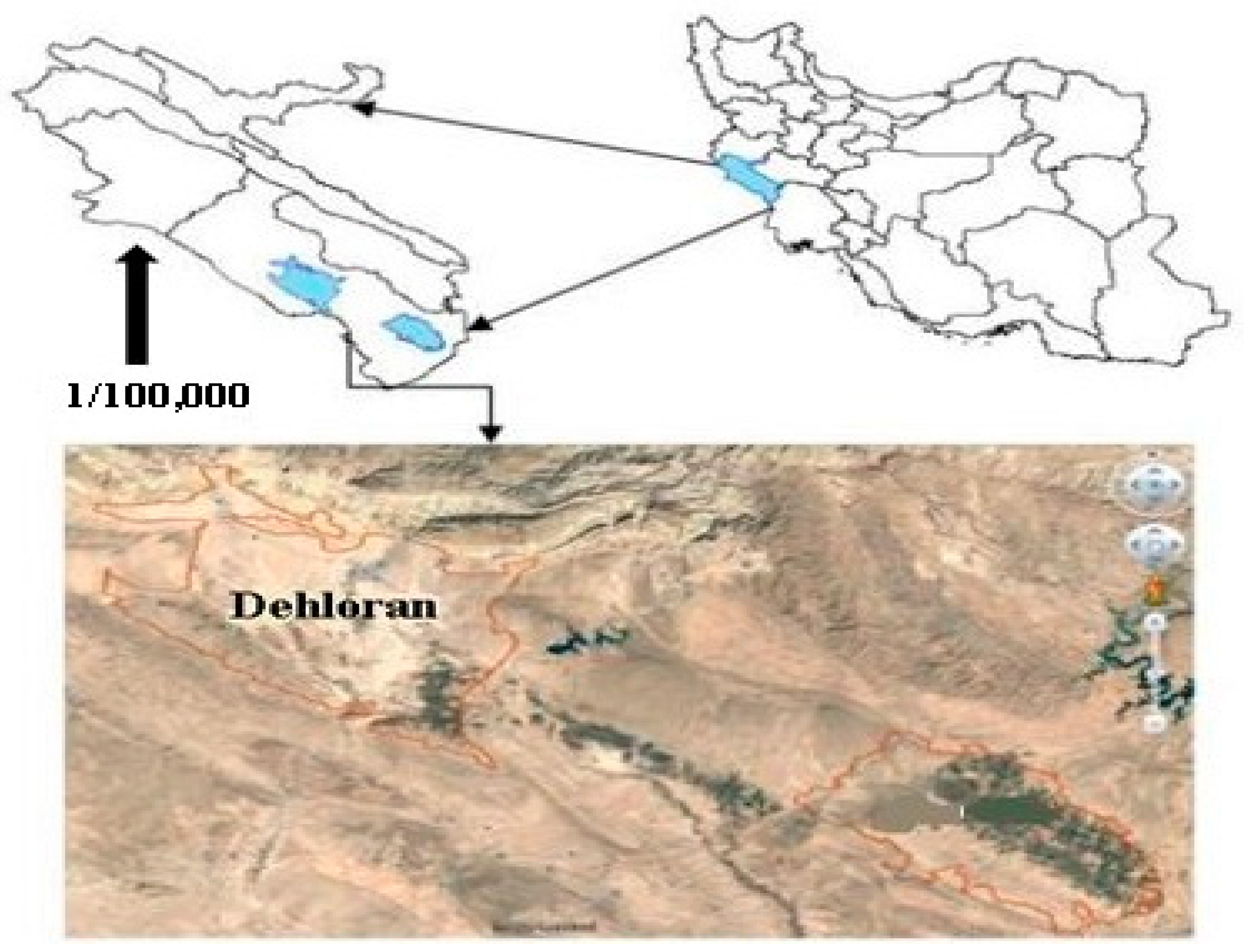
The model inputs include four categories: climate, plants, soil, and management. The input data in the region include the maximum and minimum air temperature (°C), the amount of rainfall (mm·day⁻¹), reference evapotranspiration (ET_o) (mm·day⁻¹), and the average annual concentration of carbon dioxide (CO₂) (ppm).

The input data can be those obtained on a daily basis, ten-day basis, or monthly basis. To obtain the reference evapotranspiration calculated from these parameters, the ET_o Calculator was used. The data required by this calculator include the minimum and maximum temperatures, relative humidity, wind speed, and the number of hours of sunshine.

The most important input data in the plant category include: 1. the type of plant (fruit or seed crops, leafy vegetables, or root or tuberous plants and C3 or C4); 2. the planting method (seed or seedling); 3. the planting date; 4. the growth period (days); 5. plant development information (early-stage vegetation (CCo), plant celestial development, flowering and seed formation, plant root depth development, temperature, and plant density estimation); 6. plant information in conditions without water stress, fertilizer, and salinity, which includes water use efficiency data (WP*) and the crop harvest index (HI), where the reference harvest index (HI_o) is presented as a representative of the harvest index; 7. water (coefficients and the pattern of water absorption); 8. the pattern of water extraction by roots; and 9. the parameters of water irrigation under stress conditions. Data entry for each category above was in accordance with the defined projects.

2.2. The study Area

The study area of the Dehloran plain is 54,755 hectares in Dehloran city, located in Ilam Province (with a longitude of 47′17 to 47′22 and a latitude of 32′32 to 32′37). In this region, the long-term average rainfall is 262 mm, with a maximum monthly rainfall of 50 mm of precipitation in January and a minimum rainfall of 0 mm during the summer. The average maximum monthly temperature in this region is 42.6 °C in August, and the average minimum monthly temperature is 8.3 °C in January.

To validate the model, highly transparent data were used from twenty observed fields (Figure 1).

2.3. Plant Data

The plant data and crop characteristics include constant parameters and user-specific data. The values of constant plant parameters do not change over time or among geographic situations and are present in the model by default for important crops, including wheat. These constant parameters are calibrated with no limitations using plant growth data in favorable conditions and are used with the stress response factor under water stress conditions. In addition to constant parameters, some other data required for the simulation are dependent on the crop species and/or have different values according to various managerial and environmental conditions. Some of these parameters include the cultivation date and density, the timing of plant phenological stages, and maximum root depth, which are variable depending on the specific conditions of each region and crop and are determined by the user (

Table 1. Growth period duration and the planting/growing dates of the crop.

Crop	Growth Period (Days) in Different Stages					Planting Date	Date of Harvest
	Vegetative Growth	Flowering	Seeding	Granulation	Senescence
Winter wheat	30	60	70	20	180	The second half of November	The second half of May
Barley	20	60	70	20	170	The second half of November	The third half of April

).

2.4. Irrigation and Field Management

These data include two parts, irrigation and field management, and the latter consists of selecting the soil fertility level, the method of soil water balance, such as mulch to reduce soil evaporation or mounds to save water in the field, and the plowing method. For irrigation management, rain-fed or irrigated crops are selected by the user. An irrigation system was selected in this research, and part of the wet and defined level was applied to detect the water quality, time, and level of irrigation. Basin irrigation was selected based on the commonly used irrigation method in the region. No mounds or mulch was used in field management. Six irrigation treatments, namely, full irrigation (100% (T100)) and 90% (T90), 80% (T80), 70% (T70), 60% (T60), and 50% (T50) water requirements (

Table 2. Estimation of the water requirements of the planting patterns.

Crop	Maximum Depth of Root Development (cm)	Net Volume of Irrigation Water (m3)	Gross Volume of Irrigation Water (m3)	Net Need for Irrigation Cycle (mm)	Gross Need for Irrigation Cycle (mm)	Maximum Hydromodule (lit·s−1)	Number of Irrigations
Winter wheat	120	3789	6888	63	115	1.15	6
Barley	100	3092	5622	62	113	1.04	5

). The experimental design used in this research is considered a completely randomized block design; the output of Cropwat results is annual, but the calculations pertain to 2 years, which exactly corresponds to the 2-year period of crop cultivation.

2.5. Meteorological Data

In the AquaCrop model, the required meteorological data include precipitation, minimum/maximum temperatures, reference evapotranspiration, and atmospheric CO₂ concentration. Data obtained from the Ilam meteorological station were used in this study. The default atmospheric CO₂ concentration from 1902 to 2099 was used in the model. The reference plant evapotranspiration was calculated using the ET_o Calculator tool in the AquaCrop model [1] (

Table 3. Climatic characteristics over a 20-year statistical period (1999–2019) in Dehloran.

Month	ET (mm·day−1)	Sunny Hours	Wind Speed (Km·day−1)	Humidity (%)	Maximum Temperature (°C)	Minimum Temperature (°C)	Effective Rainfall (mm)	Rainfall (mm)
January	1.93	6.3	164	59	18.1	8.8	33.5	41.9
February	3.01	7.2	181	48	22.7	12.1	24.2	30.3
March	4.66	7.7	225	42	28.4	16.6	28.3	35.4
April	5.98	8.2	181	32	35.4	22.9	18.3	22.9
May	10.01	10.7	302	22	42.7	29.1	0.1	0.1
June	10.83	11.3	294	20	45.6	31.7	0	0
July	10.28	10.9	259	20	46.6	32	0	0
August	10.28	10.7	251	21	43.4	28.7	1.1	1.4
September	7.05	9.2	216	26	37.4	24	2.5	3.1
October	4.21	7.1	181	43	28.1	16.9	22.7	28.4
November	2.3	6.3	147	58	20.4	10.8	39.5	49.4
December	1.69	6.2	147	63	17.4	8.3	39.5	49.4

).

2.6. Soil Properties

In this section, the required data include the texture and layers of soil, electrical conductivity (EC) of saturated soil, volumetric water content, field capacity, and permanent wilting point. The model can estimate the EC of unsaturated soil using soil water content data (

Table 4. Soil input data for the model.

Soil	Value
Soil type	Lumi Sandy
Saturated hydraulic conductivity (mm·day−1)	1200
Saturated moisture (V %)	41
Crop capacity point (V %)	22
Permanent wilting point (V %)	10
Thickness of soil layer (m)	2.5
Soil penetration coefficient	46
Bulk density (gr·cm−3)	1.4

).

2.7. Model Calibration

Calibration involves changing some of the parameters and coefficients of the model so that the data simulated by the model are in acceptable agreement with observed or field data. In this study, the model was calibrated based on data from the first year of cultivation (2018), and output data simulated by the model were compared with observed data or actual changes and expressed as a model coefficient. This was carried out until the observed and simulated data had acceptable error estimates. Climate data measured for plants, soil, and farm management were entered into the model. Then, some of the best-fit model coefficients between observed and simulated yield values were reduced or increased.

One of the critical factors in plant model calibration is the calibration of the canopy cover (CC). Furthermore, the growth rate of the crop shell or cover is calculated by the model after entering the phenological dates of the plant, such as the time of emergence, the time when reaching the maximum canopy coverage (CCx), the time of the onset of aging, and the maturity and ripening of the crop. The canopy growth coefficient (CGC), loss coverage ratio (CGC), and water stress profiles are the main factors in estimating vegetation. The parameters of the water stress curve in relation to default data within the model can be changed to best fit observed and simulated data (

Table 5. Plant parameters used in the model for wheat and barley simulation.

Crop Characteristics		Crop		Unit
		Winter Wheat	Barley
Crop type		Root	Root
Planting method		Sowing	Sowing
Category of the plant in terms of carbon		C3	C3
Cropping period		22 October	22 October
Length of growing cycle		180	170	Days
Canopy development	Canopy growth coefficient (CGC)	18.40	11	% inc. in CC relative to existi. CC per GDD
	Canopy decline coeff. (CDC) at senescence	8.70	9.40	%; decrease in CC relative to CCx per GDD
	Canopy cover (CCo)	6	6	% at 90% emergence
	Maximum canopy cover	93	93	CCx (%)
	Shading surface during germination	1.50	1.50	cm2
Growing cycle	Germination	30	20	day
	Flowering	60	60	day
	Granulation period	90	70	day
	Senescence	110	90	day
Root deepening	Min.	0.20	0.20	m
	Max.	1.20	1.00	m
	Time to reach maximum root depth	70	70	Day
Temperature	Base temperature	0	0	°C
	Cut-off temperature	30	15	°C
	Minimum degree of pollination	5	5	°C
	Maximum degree of pollination	35	35	°C
Harvest Index			50	%
Soil water drainage deduction for vegetation development	P(upper)	0.25	0.25	At this amount, vegetative growth stops
	P(lower)	0.60	0.60	At this amount, vegetative growth stops
Upper threshold of stomatal conductance	P(upper)	0.65	0.65	Above this, stomata begin to close
Upper threshold of senescence stress	P(upper)	0.65	0.65
Canopy growth factor		5	3
Stomatal control method factor		2.50	3
Transpiration	Transpiration coefficient at maximum coverage	1.15	1
	Effect of canopy on reducing evaporation at the end of growth	50	50	%
	Percentage decrease in Kc with age	0.15	0.13	%
Irrigation method	Furrow irrigation
Available water		70	70
Number of irrigations		6	5
Salinity stress	Upper limit threshold of salinity stress	15	15	ds·m−1
	Salinity threshold decreases yield	6	7	ds·m−1

).

2.8. Model Validation and Performance Evaluation

In the validation phase, the calibration model performance was evaluated. For this study, field data from the second year of cultivation (2019) were used. The output data from the model were compared with the observed data. To evaluate the performance of the model, statistical methods, such as the best fit of the regression line between observed and simulated data and comparison with the 1:1 line, the coefficient of determination (R²), root-mean-square error (RMSE), normalized root-mean-square error (NRMES), and Wilmot index, were used.

The statistical indicators of the quality of the model (EF) are dimensionless, and an indicator of the relative magnitude of the measured residual variance with a value close to zero or negative indicates that the model provides a good prediction from the observed data.

Given that the RMSE value depends on the unit of measurement, the evaluation of different models for two variables with different units will not be correct. Hence, the RMSE values are divided into dependent variable ranges. This is named the normalized RMSE (NRSME). This criterion is appropriate for the comparison of different models. To compare field data with those of the model, the testing of the model parameters and the output results is required. For this purpose, and in order to compare overlapping models, we used the F-test with a degree of freedom of n − 1 and a significance level of 95%. In the F-test, when the absolute computational value is less than the critical absolute value, we can accept the null hypothesis (H0) and reject hypothesis 1 (H1).

$$\mathrm{RMSE}=\sqrt{(\frac{1}{n}}{{\displaystyle \sum }}_{i=1}^n{\left(S_i-O_i\right)}^2)$$

(2)

$$\mathrm{NRMSE}=\frac{1}{Oavg}\sqrt{(\frac{1}{n}}{{\displaystyle \sum }}_{i=1}^n{\left(S_i-O_i\right)}^2)\times 100$$

(3)

$$\mathrm{EF}=1-\frac{{{\displaystyle \sum }}_{i=1}^n{\left(O_i-S_i\right)}^2}{{{\displaystyle \sum }}_{i=1}^n{\left(O_i-O_{avg}\right)}^2}$$

(4)

$$\mathrm{d}=1-\frac{{{\displaystyle \sum }}_{i=1}^n{\left(S_i-O_i\right)}^2}{{{\displaystyle \sum }}_{i=1}^n{\left(\left|S_i-O_{avg}\right|+\left|O_i-O_{avg}\right|\right)}^2}$$

(5)

where “n” is the number of data, “S_i” is the simulated data, “O_i” is the observed data, and “O_avg” is the observed average data.

2.9. Sensitivity Analysis of Input Data

The simulated results were subjected to sensitivity analysis to determine the effect of the input data used in the model calibration test. Grain yield, biomass, vegetation, and plant water use efficiency (WUE) were considered the input data (

Table 6. The results of model calibration for grain yield, biomass, and water use efficiency for the winter wheat crop under different irrigation conditions (2018).

Treatment	Yield (ton/ha)		Pe	Biomass (ton/ha)		Pe	WP (kg·m−3)		Pe
	Obs.	Sim.	(±%)	Obs.	Sim.	(±%)	Obs.	Sim.	(±%)
T100	4.50	4.69	4.22	8.837	8.668	1.91	0.66	0.682	3.33
T90	4.037	4.21	4.29	8.357	8.198	1.90	0.71	0.74	3.04
T80	3.677	3.79	3.07	7.482	7.727	3.27	0.79	0.814	8.86
T70	3.200	3.29	2.81	6.951	7.181	3.30	0.85	0.87	2.35
T60	2.918	3.01	3.15	6.315	6.503	2.97	0.92	0.951	3.37
T50	2.583	2.65	2.59	5.584	5.859	4.92	1.13	1.08	4.42

Note: P_e: Simulation error.

). Accordingly, the model input data were categorized according to their effects on the model inputs based on the degree of sensitivity (high, moderate, and low). In this study, three classes were used: the first is a 15% change in the output values of the model, defined as very sensitive data; the second is a change from 5% to 15% in the output values, defined as semi-sensitive; and the third is a change of less than 5% in the output data, considered data with a low sensitivity coefficient [1,18,21].

3. Results

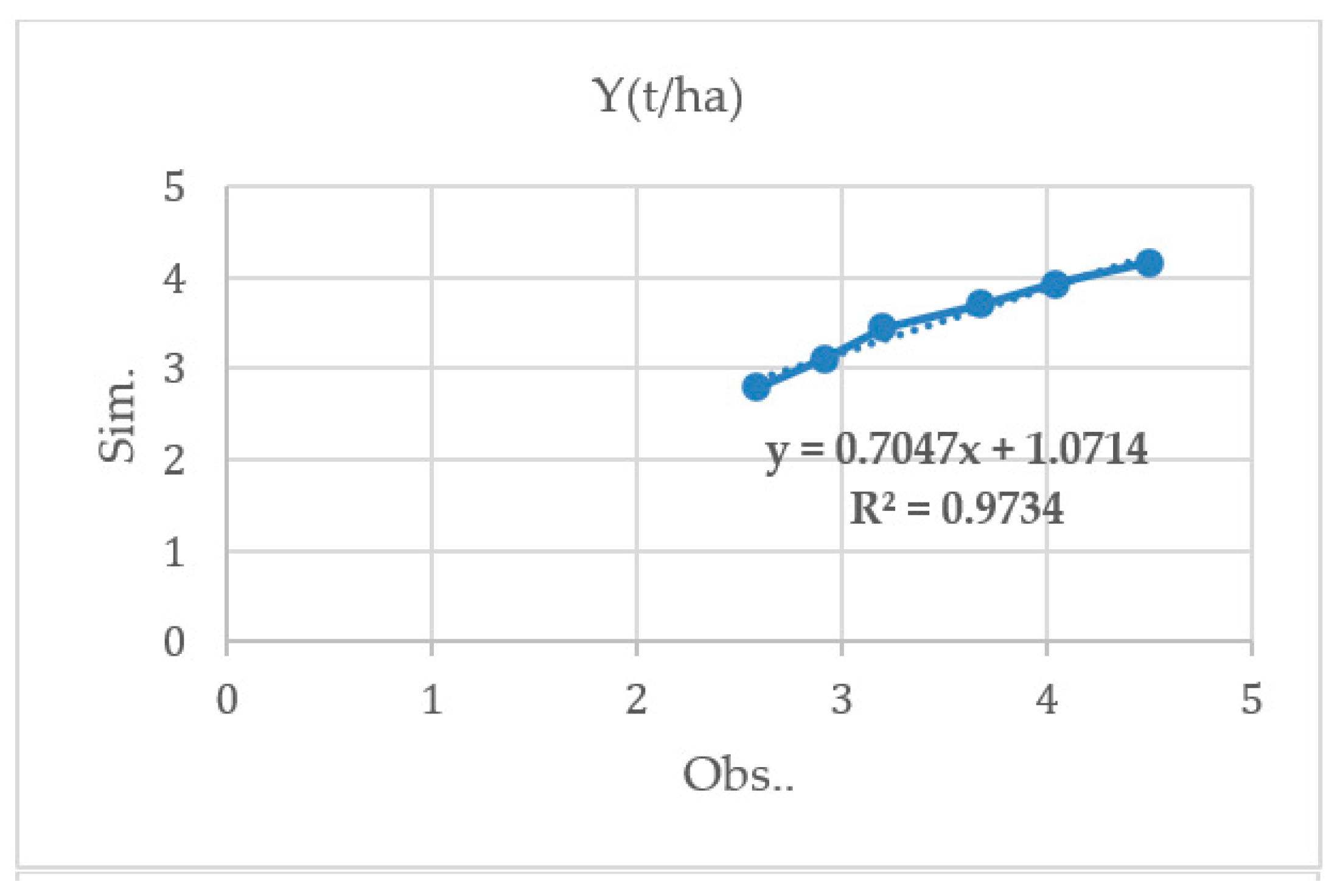
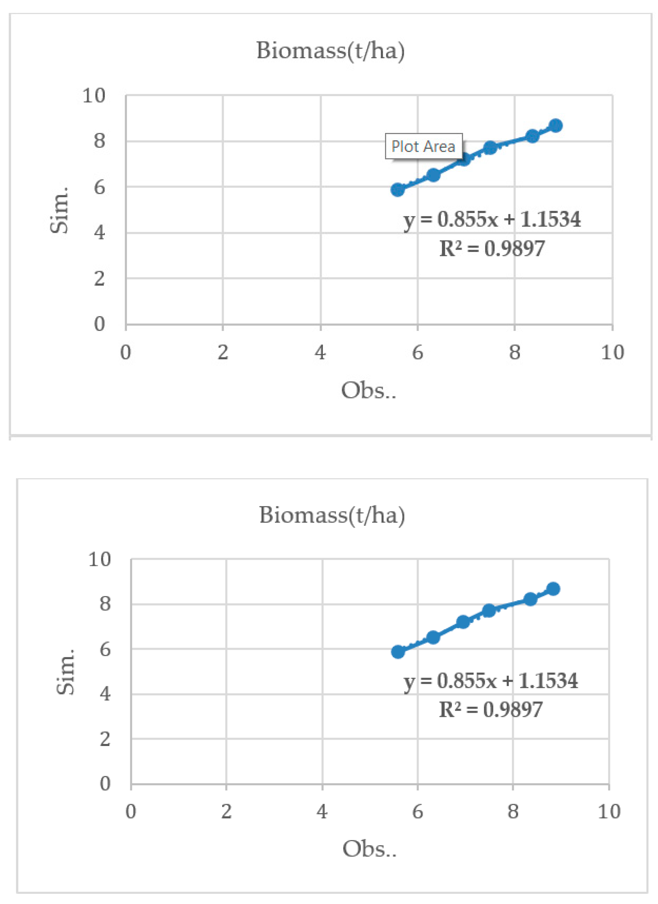
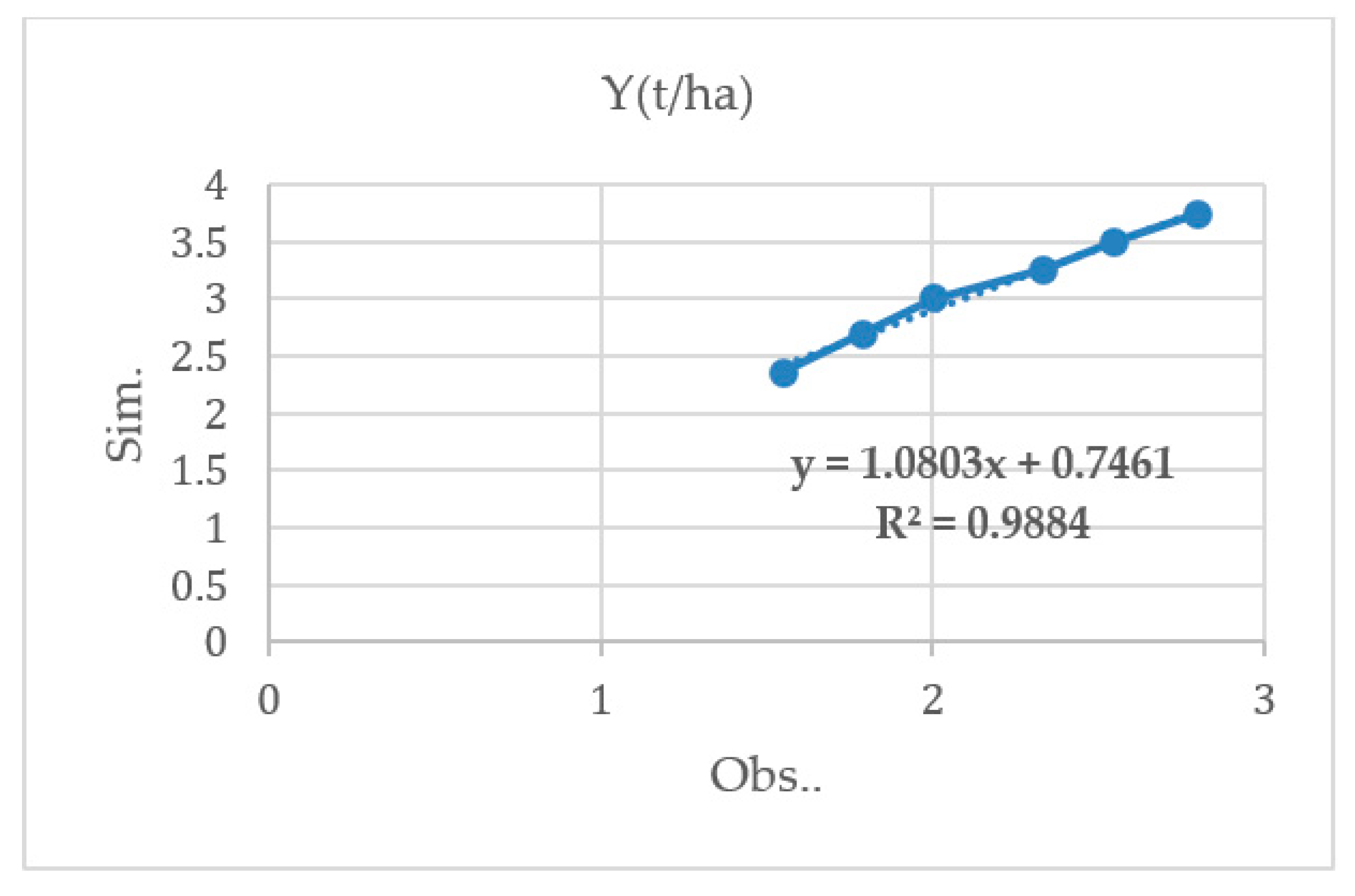
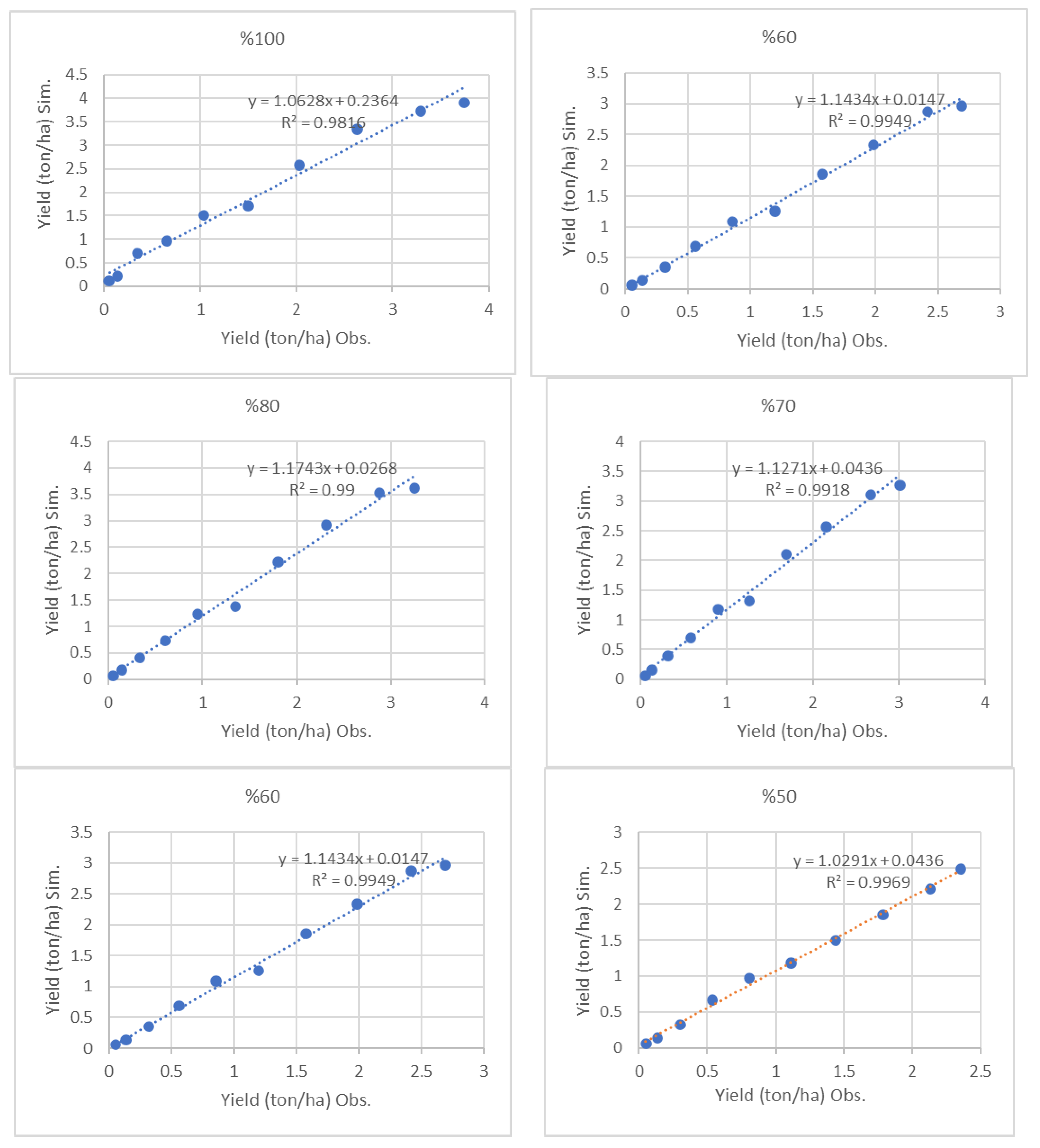
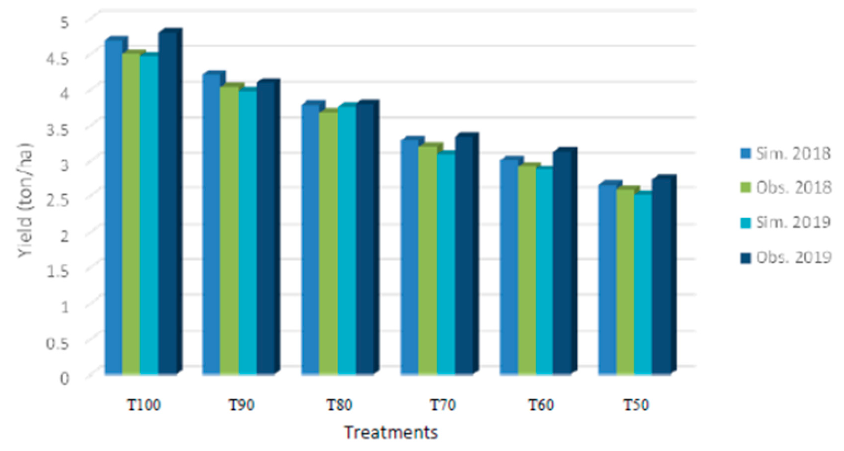
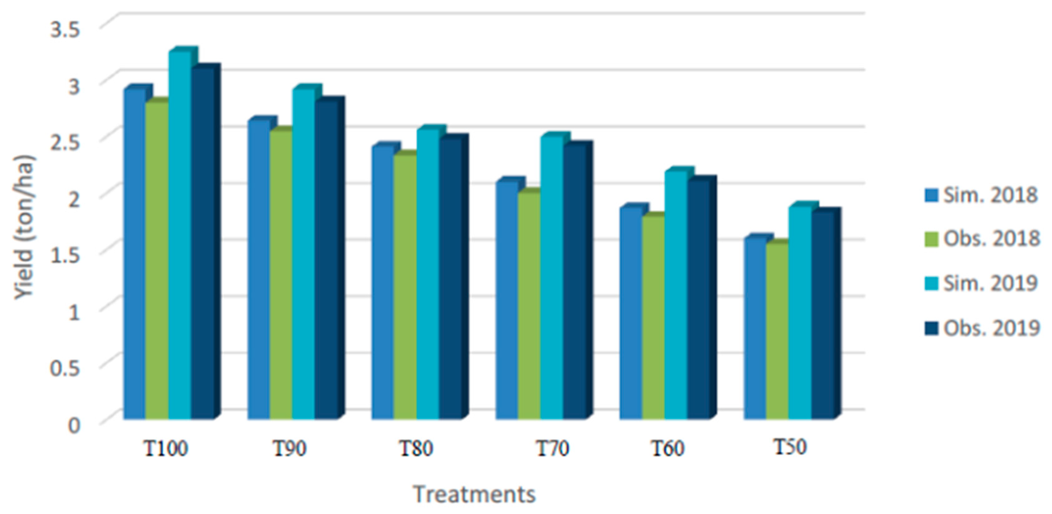
3.1. Model Performance Evaluation

The simulation results for grain yield, biomass, and water use efficiency produced by the model compared with the data observed in the calibration test using different irrigation levels for winter wheat plants are listed in Table 6.

Table 7. The results of model calibration for grain yield, biomass, and water use efficiency for the barley crop under different irrigation conditions (2018).

Treatment	Yield (ton/ha)		Pe	Biomass (ton/ha)		Pe	WP (kg·m−3)		Pe
	Obs.	Sim.	(±%)	Obs.	Sim.	(±%)	Obs.	Sim.	(±%)
T100	2.80	2.92	4.29	11.71	11.34	3.16	0.71	0.74	4.23
T90	2.548	2.64	3.61	10.84	10.599	2.22	0.76	0.79	3.95
T80	2.335	2.41	3.21	9.721	9.857	1.40	0.84	0.82	2.38
T70	2.002	2.1	4.90	8.863	9.112	2.81	0.87	0.90	3.45
T60	1.79	1.87	4.47	7.947	8.183	2.97	1.02	1.06	3.92
T50	1.55	1.6	3.23	6.882	7.195	4.55	1.06	1.10	3.77

Note: P_e: Simulation error.

lists the same values for winter barley plants. The results show that the minimum and maximum errors for winter wheat are 1.90% when estimating the grain yield with 90% irrigation and 4.92% when estimating water use efficiency with 50% deficit irrigation. For barley, the minimum and maximum errors are 1.40% for the estimation of water use efficiency with 80% irrigation and 4.90% for the grain yield estimation with 80% deficit irrigation.

Using the functions represented in Figure 1 and Figure 2, the test calibration of the model performance to simulate grain yield resulted in values of R², RMSE, d, EF, and NRMSE equal to 0.97, 3, 0.98, 0.94, and 4 for winter wheat, respectively, and 0.98, 4, 0.92, 0.89, and 7 for barley; thus, it can be concluded that the model is ideal. According to the results, it can be concluded that the accuracy of the model decreases with increasing water stress. The calibration results of the model for simulating grain yield, biomass, and water use efficiency under different irrigation treatments are presented in Figure 2 for the winter wheat crop and in Figure 3 for the barley crop.

Production performance curves were generated to determine the irrigation water productivity index, and the performance of the functions were used. The functions of the relationship between productivity and the water used during the irrigation season are shown. When interpreting the points on the curve and production functions, a limitation to bear in mind is that the equation is true only in a certain range. In addition, each crop of any plant in any climate has its own function, and it is necessary to apply the results only to the same climate or the same conditions, with each plant having its own curve.

Figure 4 illustrates the production yield of wheat, and Figure 5 shows the production yield of barley with the amount of water applied to the land under different irrigation treatments. For each scenario, the required water depth was measured through Microflumes installed in the field. The water requirements of winter wheat and barley were calculated to be 415 and 391.3 mm, respectively. The levels of deficit irrigation applied to the plant during different growth periods were calculated using the product method [22]. As accurately represented by the curves, the slopes are initially high and then gradually decrease. This implies that water usage efficiency is higher for deficit irrigation strategies. When increasing the amount of irrigation, the corresponding curve finally reaches its peak. After that, further irrigation does not significantly change productivity. Due to the use of water during the germination and early growth of the plant, the curves do not start from the origin of the plot axis.

By examining and comparing the coefficients of efficiency for the performance of the product for both winter wheat and barley, including a common fuel utilization factor, among the scenarios of irrigation, scenarios with more irrigation were found to have a higher yield (Figure 6 and Figure 7).

3.2. Model Validation Results

Tests to validate the model were performed using data from the second year of cultivation (2019), and calibration was performed using planting data from the first year (2018). The results show that the minimum and maximum error estimates for the winter wheat grain yield amount to 1.05% when irrigation is 80% and 39.98% when irrigation is 50%. Furthermore, the minimum and maximum error estimates for the amount of biomass in the atmosphere are 0.95% when irrigation is 80% and 38.46% when irrigation is 50% (

Table 8. The results of model validation for grain yield, biomass, and water use efficiency for the winter wheat crop under different irrigation conditions (2019).

Treatment	Yield (ton/ha)		Pe	Biomass (ton/ha)		Pe	WP (kg·m−3)		Pe
	Obs.	Sim.	(±%)	Obs.	Sim.	(±%)	Obs.	Sim.	(±%)
T100	4.8	4.47	6.87	9.14	8.97	1.86	0.73	0.75	2.74
T90	4.1	3.98	2.93	8.87	8.70	1.91	0.76	0.79	3.95
T80	3.8	3.76	1.05	7.93	7.67	3.28	0.84	0.87	3.57
T70	3.34	3.09	7.48	7.48	7.24	3.21	0.91	0.95	4.40
T60	3.13	2.87	8.3	7.07	6.87	2.83	0.98	1.03	5.10
T50	2.73	2.51	8.06	6.62	6.32	4.53	1.18	1.22	3.39

and

Table 9. The results of model validation for grain yield, biomass, and water use efficiency for barley crop under different irrigation conditions (2019).

Treatment	Yield (ton/ha)		Pe	Biomass (ton/ha)		Pe	WP (kg·m−3)		Pe
	Obs.	Sim.	(±%)	Obs.	Sim.	(±%)	Obs.	Sim.	(±%)
T100	3.1	3.25	4.84	12.3	12.00	2.44	0.74	0.778	5.14
T90	2.81	2.92	3.91	11.46	11.28	1.57	0.79	0.82	3.8
T80	2.48	2.56	3.23	10.47	10.37	0.95	0.87	0.91	4.6
T70	2.42	2.50	3.31	9.86	9.65	2.13	0.91	0.962	5.71
T60	2.11	2.19	3.79	8.77	8.57	2.28	1.1	1.152	4.73
T50	1.83	1.88	2.73	7.62	7.36	3.41	1.17	1.22	4.27

).

In addition, the efficiency of the model in the validation experiment was obtained for simulating grain yield, where R², RMSE, d, EF, and NRMSE are equal to 0.99, 4, 0.97, 0.93, and 4.4 for winter wheat, respectively, and 0.97, 7, 0.94, 0.91, and 9 for barley.

Using the data in Figure 8 and Figure 9 for all scenarios of irrigation, the F-test was performed in order to compare the variance between the field data and plant models for both winter wheat and barley products at a 95% significance level (

Table 10. F-test results of field data and model for winter wheat and barley crops.

Absolute Value of the Critical Point of Winter Wheat: 3.43 Absolute Value of the Critical Point of Barley: 3.17		Hypothesis H0: Yij = Yji H1: Yij ≠ Yji
Significance Level: 0.05
Irrigation scenarios	Absolute value of F statistic	Absolute value of F statistic
	Winter Wheat	Barley
50%	1.15	1.06
60%	1.18	1.31
70%	1.10	1.28
80%	1.13	1.39
90%	1.15	1.30
100%	1.06	1.15

Note: Source: Research Findings.

).

Figure 10 and Figure 11 display the comparisons of the observed and simulated performance (ha) for winter wheat and barley crops during the years 2018 and 2019 at different levels of water stress.

4. Discussion

Field measurements over a large area with arid and semiarid climatic conditions were used in this study. To validate the model, highly transparent data were used on twenty observed fields. On the one hand, a large area of Iran has an arid or semiarid climate. On the other hand, the water that agriculture needs is a limiting factor. Therefore, it seems that the AquaCrop model used in this study is suitable for studying the production function of two strategic products that are cultivated at a very high level in Iran, along with an approach to increasing water use efficiency per yield. In this study, the AquaCrop models accurately simulated crop canopy cover (CC), biological yield (BY), and grain yield (GY) under both regular and deficit irrigation. In water-limited environments, the AquaCrop model is a potentially valuable tool to use for maximizing winter wheat and barley yields in the region.

This study’s results illustrate that the current scenario-based policies for agriculture with 100% irrigation increase crop yield in existing conditions. Furthermore, with less irrigation, not only is productivity not reduced, but the percentage deficit in the amount of irrigation to save water instead increases productivity and the water efficiency factor by a notable degree.

AquaCrop models enable the simulation of transpiration during the growing season, yield, crop water requirements, and water use efficiency based on required water, climate, soil, and plants. Due to the high cost of operations and field measurements, as well as time and place limitations, in this study, the AquaCrop model was calibrated by using measurement data taken on the farm. Finally, after calibration, the results could be used to estimate performance in the future; therefore, although the AquaCrop model may have some problems, it seems that it can be used after being calibrated with a series of initial data in the field, which can be easily measured. The AquaCrop model also makes it easy to compute scheduling irrigation requirements, water consumption, and irrigation intervals, and compared to other plant models, the AquaCrop model requires less input data. Based on existing statistics, it is capable of accurately evaluating and simulating plant growth. The calibration of model parameters related to water stress, the crop canopy, and the reference harvest index at default values is required, as changes in these variables can be caused by the use or climate of the study area.

5. Conclusions

In reviewing the results of the calibration and validation of field data using the model, it is concluded that the percentage error in the estimations of grain yield, biomass, and water use efficiency in deficit irrigation scenarios increases with the decreasing amount of water required by the plant. The results of calibration and validation errors during the crop years 2018 and 2019 for yield, biomass, and water use efficiency were close in magnitude.

To determine an optimal irrigation level, data measured in different irrigation scenarios (full irrigation or 100% water requirement and 90, 80, 70, 60, and 50% irrigation) were calibrated and validated for arid and semiarid climatic conditions using the AquaCrop model. The model was calibrated to simulate the grain yields of winter wheat and barley using R², RMSE, d, EF, and NRMSE statistical indicators. The obtained values of these indices were, respectively, 0.97, 3, 0.98, 0.94, and 4 for winter wheat and 0.98, 4, 0.92, 0.89, and 7 for barley. The model efficiency was also validated using crop harvest data in the crop year 2019. For the grain yield simulation, the calculated values of R², RMSE, d, EF, and NRMSE statistical indicators were, respectively, 0.99, 4, 0.97, 0.93, and 4.4 for winter wheat and 0.97, 7, 0.94, 0.91, and 9 for barley. The data of field and modeled samples were analyzed by analysis of variance (ANOVA) using the F-test, and significant results were obtained for both crops in all applied scenarios at the 95% level. The AquaCrop model can be used to predict and optimize winter wheat and barley yields and water productivity under different irrigation treatments in Illam.

References

1. Abedinpour, M. Agricultural Water Management with AquaCrop Model, 1st ed.; Isfahan University Jahad Publications: Isfahan, Iran, 2019; pp. 11–18, 81–86, 210–219. [Google Scholar]
2. Saab, M.A.; Albrizio, R.; Nangia, V.; Karam, F.; Rouphael, Y. Developing scenarios to assess sunflower and soybean yield under different sowing dates and water regimes in the Bekaa valley (Lebanon): Simulations with Aquacrop. Int. J. Plant Prod. 2014, 8, 1735–6814. [Google Scholar] [CrossRef]
3. Hamidreza, S.; Mohd, A.M.S.; Teang, S.L.; Sayed, F.M.; Arman, G.; Mohd, K.Y. Application of AquaCrop model in deficit irrigation management of Winter wheat in arid region. Afr. J. Agric. Res. 2011, 6, 2204–2215. [Google Scholar]
4. Shirshahi, F.; Babazadeh, H.; Ebrahimipak, N.; Zeraatkish, Y. Calibration and evaluation of the performance of Aquacrop model in managing the amount and time of deficit Irrigation in wheat. Iran. J. Irrig. Sci. Eng. 2017, 41, 31–44. (In Persian) [Google Scholar]
5. Sema, K.A.L.E.; Madenoğlu, S. Evaluating AquaCrop Model for Winter Wheat under Various Irrigation Conditions in Turkey. J. Agric. Sci. 2017, 24, 205–217. [Google Scholar]
6. Ahmadi, S.H.; Mosallaeepour, E.; Kamgar-Haghighi, A.A.; Sepaskhah, A.R. Modeling Maize Yield and Soil Water Content with AquaCrop Under Full and Deficit Irrigation Managements. Water Resour. Manag. 2015, 29, 2837–2853. [Google Scholar] [CrossRef]
7. Ramezani, M.; Babazadeh, H.; Sarai Tabrizi, M. Simulating Barley Yield under Different Irrigation Levels by using AquaCrop Model. Irrig. Sci. Eng. (JISE) 2019, 41, 161–172. [Google Scholar] [CrossRef]
8. Goosheh, M.; Pazira, E.; Gholami, A.; Andarzian, B.; Panahpour, E. Improving Irrigation Scheduling of Wheat to Increase Water Productivity in Shallow Groundwater Conditions Using Aquacrop. Irrig. Drain. 2018, 67, 738–754. [Google Scholar] [CrossRef]
9. Hellal, F.; Mansour, H.; Abdel-Hady, M.; El-Sayed, S.; Abdelly, C. Assessment water productivity of barley varieties under water stress by AquaCrop model. AIMS Agric. Food 2019, 4, 501–517. [Google Scholar] [CrossRef]
10. Khoshravesh, M.; Mostafazadeh-Fard, B.; Heidarpour, M.; Kiani, A.-R. AquaCrop model simulation under different irrigation water and nitrogen strategies. Water Sci. Technol. 2013, 67, 232–238. [Google Scholar] [CrossRef] [PubMed]
11. Masasi, B.; Taghvaeian, S.; Gowda, P.H.; Warren, J.; Marek, G. Simulating Soil Water Content, Evapotranspiration, and Yield of Variably Irrigated Grain Sorghum Using AquaCrop. JAWRA J. Am. Water Resour. Assoc. 2018, 55, 976–993. [Google Scholar] [CrossRef]
12. Hoseinzadeh, S.; Astiaso Garcia, D. Techno-economic assessment of hybrid energy flexibility systems for islands’ decarbonization: A case study in Italy. Sustain. Energy Technol. Assess. 2022, 51. [Google Scholar] [CrossRef]
13. Hoseinzadeh, S.; Ghasemi, M.H.; Heyns, S. Application of hybrid systems in solution of low power generation at hot seasons for micro hydro systems. Renew. Energy. 2020, 160, 323–332. [Google Scholar] [CrossRef]
14. Mousavizadeh, S.; Honar, T.; Ahmadi, S. Assessment of the AquaCrop Model for simulating Canola under different irrigation managements in a semiarid area. Int. J. Plant Prod. 2016, 10, 425–445. [Google Scholar] [CrossRef]
15. He, Q.; Li, S.; Hu, D.; Wang, Y.; Cong, X. Performance assessment of the AquaCrop model for film-mulched maize with full drip irrigation in Northwest China. Irrig. Sci. 2020, 39, 277–292. [Google Scholar] [CrossRef]
16. Amiri, A.; Bahrani, S.; Irmak, N.; Mohammadiyan, R. Evaluation of irrigation scheduling and yield response for wheat cultivars using the AquaCrop model in an arid climate. Water Supply. 2021, 22, 602–614. [Google Scholar] [CrossRef]
17. Kheir, A.M.S.; Alkharabsheh, H.M.; Seleiman, M.F.; Al-Saif, A.M.; Ammar, K.A.; Attia, A.; Zoghdan, M.G.; Shabana, M.M.A.; Aboelsoud, H.; Schillaci, C. Calibration and Validation of AQUACROP and APSIM Models to Optimize Wheat Yield and Water Saving in Arid Regions. Land 2021, 10, 1375. [Google Scholar] [CrossRef]
18. Kheir, A.M.; Hoogenboom, G.; Ammar, K.A.; Ahmed, M.; Feike, T.; Elnashar, A.; Liu, B.; Ding, Z.; Asseng, S. Minimizing trade-offs between wheat yield and resource-use efficiency in the Nile Delta–A multi-model analysis. Field Crop. Res. 2022, 287. [Google Scholar] [CrossRef]
19. Shen, X.; Wang, G.; Zeleke, K.T.; Si, Z.; Chen, J.; Gao, Y. Crop Water Production Functions for Winter Wheat with Drip Fertigation in the North China Plain. Agronomy 2020, 10, 876. [Google Scholar] [CrossRef]
20. Soomro, K.B.; Alaghmand, S.; Shahid, M.R.; Andriyas, S.; Talei, A. Evaluation of Aquacrop Model in Simulating Bitter Ground Water Productivity under Saline Irrigation. Irrig. Drain. J. 2019, 69, 63–73. [Google Scholar] [CrossRef]
21. Abedinpour, M.; Sarangi, A.; Rajput, T.; Singh, M.; Pathak, H.; Ahmad, T. Performance Evaluation of Aquacrop Model for Maize Crop in a Semi-Arid Environment. Agric. Water Manag. 2012, 110, 55–66. [Google Scholar] [CrossRef]
22. Najarchi, M.; Kaveh, F.; Babazadeh, H.; Manshouri, M. Determination of the yield response factor for field crop deficit irrigation. Afr. J. Agric. Res. 2011, 6, 3700–3705. [Google Scholar] [CrossRef]
Figure 1. Location map of the study area in Iran—Ilam Province.
Water 14 03455 g001
Figure 2. The results of model calibration for simulating grain yield, biomass, and water use efficiency for the winter wheat crop under different irrigation conditions.
Water 14 03455 g002aWater 14 03455 g002b
Figure 3. The results of model calibration for simulating grain yield, biomass, and water use efficiency for the barley crop under different irrigation conditions.
Water 14 03455 g003aWater 14 03455 g003b
Figure 4. The crop production yield versus the irrigation level for the winter wheat crop.
Water 14 03455 g004
Figure 5. The crop production yield versus the irrigation level for the barley crop.
Water 14 03455 g005
Figure 6. The productivity coefficient versus crop yield for the winter wheat crop.
Water 14 03455 g006
Figure 7. The productivity coefficient versus crop yield for the barley crop.
Water 14 03455 g007
Figure 8. The results of model calibration for simulating the crop yield of the winter wheat crop under different irrigation conditions.
Water 14 03455 g008
Figure 9. The results of model calibration for simulating the crop yield of the barley crop under different irrigation conditions.
Water 14 03455 g009
Figure 10. Comparison of the yield (t/ha) simulated by the AquaCrop model with values observed for the winter wheat crop at different water stress levels.
Water 14 03455 g010
Figure 11. Comparison of the yield (t/ha) simulated by the AquaCrop model with values observed for the barley crop at different water stress levels.
Water 14 03455 g011