Article

Evaluation of Soil Water Content Using SWAT for Southern Saskatchewan, Canada

1
Prairie Adaptations Research Collaborative, University of Regina, Regina, SK S4S 0A2, Canada
2
Environmental Systems Engineering, University of Regina, Regina, SK S4S 0A2, Canada
*
Author to whom correspondence should be addressed.
Water 2022, 14(2), 249; https://doi.org/10.3390/w14020249
Submission received: 12 November 2021 / Revised: 5 January 2022 / Accepted: 11 January 2022 / Published: 15 January 2022
(This article belongs to the Section Soil and Water)

Abstract

:
Soil water content (SWC) is one of the most important hydrologic variables; it plays a decisive role in the control of various land surface processes. We simulated SWC using a Soil and Water Assessment Tool (SWAT) model in southern Saskatchewan. SWC was calibrated using measured data and Soil Moisture Active Passive (SMAP) Level-4 for the surface (0–5 cm) SWC for hydrological response units (HRU) at daily and monthly (warm season) intervals for the years 2015 to 2020. We used the SUFI-2 technique in SWAT-CUP, and observed daily instrumented streamflow records, for calibration (1995 to 2004) and validation (2005–2010). The results reveal that the SWAT model performs well with a monthly PBIAS < 10% and Nash–Sutcliffe efficiency (NS) and R2 ≥ 0.8 for calibration and validation. The correlation coefficient between ground measurement with SMAP and SWAT products are 0.698 and 0.633, respectively. Moreover, SMAP data of surface SWC coincides well with measurements in terms of both amount and trend compared with the SWAT product. The highest r value occurred in July when the mean r value in SWAT and SMAP were 0.87 to 0.84, and then in June for r value of 0.75. In contrast, the lowest values were in April and May (0.07 and 0.04, respectively) at the beginning of the growing season in southern Saskatchewan. Furthermore, calibration in the SWAT model is based on a batch form whereby parameters are adjusted to corresponding input by modifying simulations with observations. SWAT underestimates the abrupt increase in streamflow during the snowmelt months (April and May). This study achieved the objective of developing a SWAT model that simulates SWC in a prairie watershed, and, therefore, can be used in a subsequent phase of research to estimate future soil moisture conditions under projected climate changes.

1. Introduction

Soil water content (SWC) is an important hydrologic state variable related to actual and potential evapotranspiration, storage and infiltration, surface runoff, and overall water balance [1,2]. From a regional perspective, SWC is a limiting factor in crop yield as water demand often exceeds precipitation amounts [3,4]. The Canadian Prairies comprise about 80% of Canada’s agricultural lands with more than 90% wheat and canola production. Southern Saskatchewan falls in the center of the region and is extremely prone to frequent and severe droughts [5]. The semi-arid conditions include low precipitation, mostly received from April through June, and high evaporation during the entire farming season. To address the issues associated with food security and to stimulate economic growth, the Saskatchewan Ministry of Agriculture has recommended 400 percent expansion in irrigated areas [6]. The recent plan to irrigate farmlands in the area requires an assessment of SWC variability across spatial and temporal scales.
The hydrography of southern Saskatchewan is a product of a dry mid-latitude continental climate, with strong seasonal and inter-annual variability, and soil landscapes formed during the most recent advance and retreat of the continental ice sheet [7]. The North and South Saskatchewan Rivers account for most of the streamflow in southern Saskatchewan. These rivers shed water from the Rocky Mountains generated by snowmelt, and, to a lesser extent, rainfall and glacier runoff. Furthermore, the rivers flow in large valleys created by meltwater from the continental ice sheet, and, thus, they are largely disconnected from the prairie runoff in terms of topography and hydrology. These unique features make hydrological modeling in the region quite complex, especially for the prediction of SWC.
The Soil and Water Assessment Tool (SWAT) is widely used for quantitative hydrological modeling [8,9,10,11,12]. This physical model is usually calibrated based on streamflow [13] but requires measured data for each variable [14,15]. Several studies have implemented remotely sensed SWC datasets to calibrate the SWAT model. Narasimhan and Srinivasan. [16] used SWAT to simulate long-term SWC using NDVI in a semi-arid area. Park et al. [17] calibrated the SWC simulated by SWAT using three databases of MODIS, Normalized Difference Vegetation Index (NDVI), and Land Surface Temperature (LST) for a forest in Spain. Havrylenko et al. [18] used NDVI and Standard Precipitation Index (SPI), and Nilawar et al. [19] used Advanced Microwave Scanning Radiometer (AMSR2). The primary limitation of these approaches is that the SWC is a site scale parameter while remote sensing is a global scale measure. Calibration is further improved through simultaneous determination of two independent variables. Uniyal et al. [2] used Landsat derived indices of Thermal Vegetation Difference Index (TVDI), NDVI, and brightness temperature (BT) along with field measurement; Rajib et al. [20] used Advanced Microwave Scanning Radiometer-Earth Observing System and field measurements. Such studies require high-resolution remote sensing data to appropriately adapt to field data.
The main objective of this research was to evaluate the reliability of the SWAT model to estimate SWC for southern Saskatchewan, Canada, using high-resolution satellite data and field measurements. Initially, sensitivity analyses were conducted to identify the relative significance of parameters affecting SWC. Next, the SWAT model was calibrated using Soil Moisture Active Passive Level-4 (SMAP L4_SM) for surface SWC and measured data. Finally, the SWC output was analyzed using field measurements and SMAP L4_SM daily and monthly data.

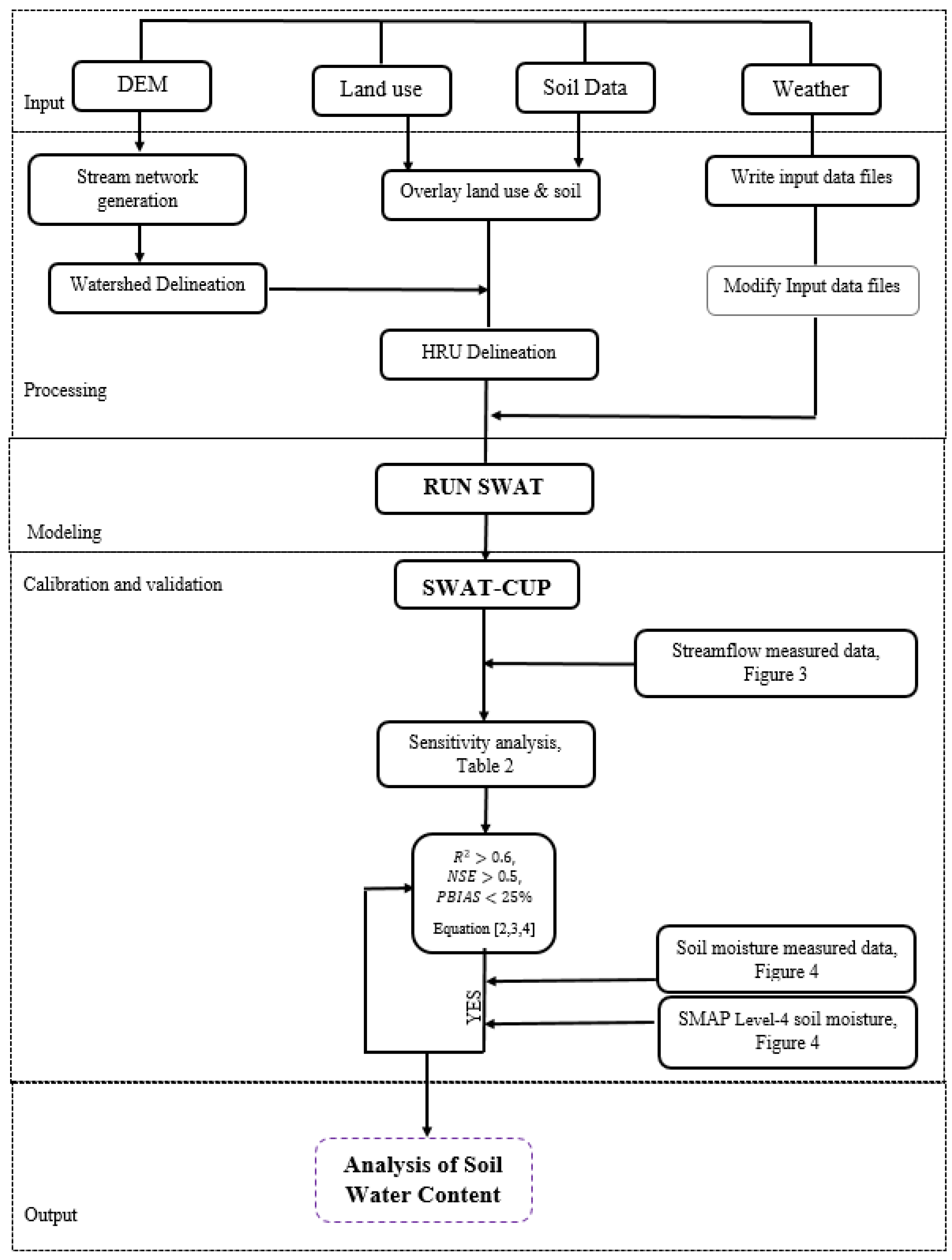
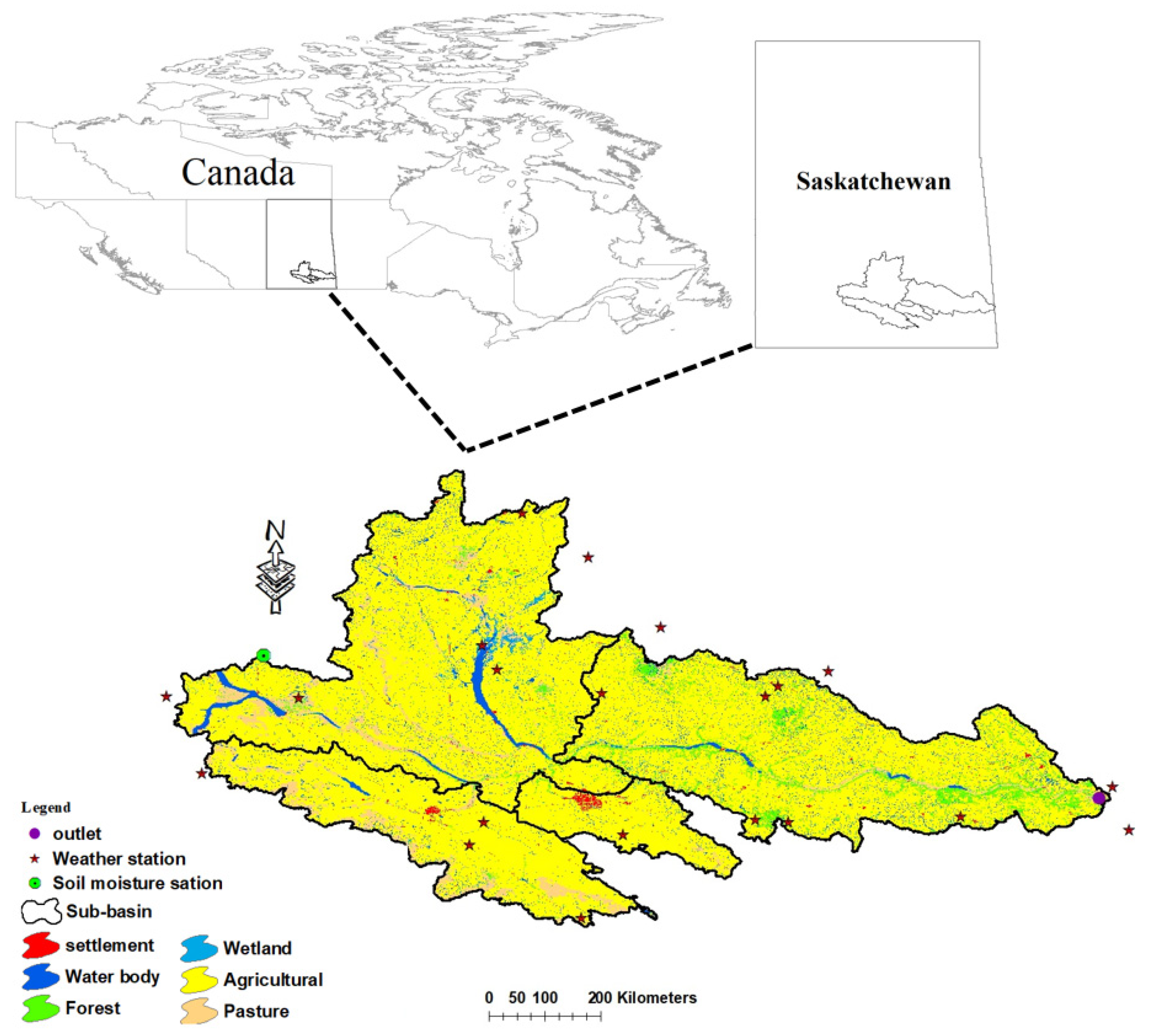
2. Research Methodology

Figure 1 gives the flow chart of the modeling process. The SWC and streamflow were evaluated for four watersheds in southern Saskatchewan (Figure 2): Lower Qu’Appelle River basin (17,800 km2) from Craven to the Manitoba border; Upper Qu’Appelle River basin (14,200 km2) comprising Lanigan-Manitou, Last Mountain Lake, and the Upper Qu’Appelle sub-basins; Moose Jaw River basin (9300 km2) including Moose Jaw; and Wascana Creek basin (3900 km2) including Regina. The region is characterized by cold dry winters and hot humid summers, with most snowmelt occurring in spring. The average annual temperature ranges from 8 °C to −3.5 °C. Agriculture is the main land use that comprises 68% cropland and 16% grassland. Approximately 70% of the area is characterized by black chernozemic soils with significant organic matter.
Table 1 summarizes the data used for hydrological modeling in the Arc SWAT interface. The spatial inputs included a land use map, soil properties description, and digital elevation model (DEM) to define HRUs. Soil type was obtained from the Soil Landscapes of Canada (SLC ver. 3.2), whereas topographic data for watershed delineation was derived from a 20 m resolution Digital Elevation Model (Canadian GeoGratis). We obtained 30 m resolution land use data for 2015 from Agriculture and Agri-Food Canada. Likewise, weather data (rainfall, solar radiation, wind speed, relative humidity, and air temperature) from 1985 to 2020 for 15 stations was obtained from Environment and Climate Change Canada. From the Water Survey of Canada (WSC) hydrometric database (HYDAT), we used daily stream discharge data for 1995–2004 for calibration and 2005–2010 for validation.
Hydrologic simulation in SWAT was based on the following water balance equation:
S W t = S W o + i = 1 t ( R d a y Q s u r f E a W s e e p Q g w ) i
S W t is final soil water content (mm), S W o is initial soil water content (mm), t is time (days), R d a y is the cumulative value of precipitation (mm), E a is actual evapotranspiration (mm), W s e e p is amount of percolation and bypass flow exiting the soil profile (mm), and Q g w is amount of return flow on day i (mm). The model calculations were performed at HRU, sub-basin, and watershed scales so that the water flow and retention variables were routed from HRUs to the sub-basins and subsequently to the watershed outlet. A total of 1441 HRUs and 27 sub-basins were delineated by defining a 5% level threshold for soil type, land use, and a uniform slope to optimize the computational time.
To calibrate SWC in the SWAT model, the Soil Moisture Active Passive (SMAP) Level-4 (L4-SM) active–passive soil moisture product was used. Recent research demonstrates various uses of SMAP in hydrological modeling: Azimi et al. [21] assimilated SMAP data in a SWAT model; Breen et al. [22] estimated soil moisture using SMAP data in a SWAT model; Li et al. [23] calibrated SMAP data in MIKE SHE as a hydrologic model; and Yi et al. [24] used SMAP data in a TOPX hydrologic model with different precipitation datasets. A discussion of interactions is beyond the scope of this study because the database is not used as an input in SWAT.
The radiometer instrument on board the SMAP observes the L-band (1.4 GHz) microwave radiation emitted from Earth’s surface. Over land, the observed radiances or brightness temperatures (Tbs) are sensitive to the moisture in the top few centimeters of the soil, provided the overlying vegetation is not too dense as is the case in southern Saskatchewan, especially in the warm season. This sensitivity is exploited in the SMAP Level-4 Soil Moisture (L4-SM) algorithm to obtain estimates of surface (0–5 cm) and root-zone (0–100 cm) soil moisture. Likewise, previous research confirms that SMAP L4 has better agreement with in situ soil moisture in croplands when compared with SMAP L3 during non-winter periods [25]. The Level-4 soil moisture and L-band brightness temperature provided 9-km resolution estimates of land surface conditions. These SWC estimates at the surface (0–5 cm) were retrieved by the SMAP radiometer at 6:00 a.m. descending and 6:00 p.m. ascending half-orbit passes [26]. The data were downloaded from NASA’s Earth Observing System Data and Information System (EOSDIS) for the summer months (April to September) in 2015–2020.
We used the Calibration and Uncertainty Program (CUP) in SWAT for sensitivity analysis (identification of parameters affecting output variance due to input variability), model calibration (parameterizing the model to local conditions to reduce prediction uncertainty), and model validation (use of calibrated parameters for comparison with observed data). Automatic calibration and validation were conducted using the Sequential Uncertainty Fitting algorithm version 2 (SUFI-2) in the SWAT-CUP [27]. The parameter uncertainty was derived from all input and output sources of uncertainty, such as the weather data, land use, and soil type.
The calibration period from 1995 to 2004 was simulated using a maximum of two batches executed with 500 SUFI-2 iterations. We evaluated the SWAT model through graphical comparison of the simulated and observed outlet streamflow hydrographs and by concurrently using three statistical criteria for goodness-of-fit: the Nash–Sutcliffe efficiency (NSE) [28]; the percent bias (PBIAS) [29]; and the Coefficient of Determination ( R 2 ) [30] according to the following equations, respectively:
NSE = [ 1 i = 1 n ( Q i o b s Q ¯ i s i m ) 2 i = 1 n ( Q i o b s Q m e a n o b s ) 2 ]  
PBIAS = i = 1 n ( Q i o b s Q i s i m ) i = 1 n Q i o b s × 100
R 2 = ( i = 1 n ( Q i o b s Q ¯ i o b s ) ( Q i s i m Q ¯ i s i m ) ) 2 ( i = 1 n ( Q i o b s Q ¯ i s i m ) ( Q i o b s Q ¯ i s i m ) ) 2 × 100
where, Q ¯ i s i m and Q ¯ i o b s are the mean monthly simulated and observed discharges, Q i o b s is observed discharge on the ith day, Q i s i m is the simulated monthly discharge, n is the total number of months, and Q m e a n o b s is the average observed monthly streamflow. After executing the first batch of calibration iterations (the first day of simulation), ‘relative’ and ‘value’ sensitivity ranking of parameters was performed by the global sensitivity analysis technique in SWAT-CUP. This allowed the optimization of the parameters by estimating their ‘relative’ and ‘value’ effect [27]. The measure of relative sensitivity among the parameters was interpreted through t-stat and p-values. The extent of the sensitivity measured by t-stat and p-value shows the significance of the sensitivity measured.
The SWC at the HRU level was extracted from the final model output. The SWC consists of soil structure elements which determine the permanent wilting point volumetric water content as a function of the clay content and bulk density in the sub-basin [2]. The wilting point was estimated according to the following equation:
W P l y = 0.4 m c × ρ b 100
where W P l y is the water content at wilting point, m c is the percent clay content of the layer (%) and ρ b is the bulk density for the soil layer ( mg   m 3 ).
Field capacity was estimated according to the following equation:
F C l y = W P l y + A W C l y
where F C l y is the water content at field capacity expressed as a fraction of the total soil volume, W P l y is the water content at wilting point, and A W C l y is the available water capacity of the soil layer. Excess water can percolate or drain, provided the temperature of the soil is above 0   ° C . We considered only the warm season because the soil layer is frozen in the other seasons in the study area. Another limitation was that SWC values in the SWAT model are not able to directly compare measured and SMAP data. To address this discrepancy, water held at the wilting point was calculated at each layer of HRU within the time frame given to the model and added to the SWAT simulated SWC following a similar approach by Rajib et al. [20] and Musyoka et al. [31]. Furthermore, SWC values in the SWAT model were spatially averaged over HRUs while field sensors were used to monitor SWC point data. To overcome this limitation, we used the average measured SWC to simultaneously compare the field measurement with L4-SM. Therefore, we used a field sensor at surface depths (0–5 cm) to compare SWC simulated in the SWAT model. Moreover, we considered the HRU at the location of this field sensor and the corresponding specific pixel of L4-SM because of the availability of a single measuring station in southern Saskatchewan.
The integrated quantities comparison of field observation with SWAT and SMAP outputs depends on the correlation coefficient (r). Generally, the relationship between two variables is considered to be strong when their r value is more than 0.7. The value of r was used to evaluate the level of correlation between two variables, i.e., SMAP and SWAT soil water content products with field measurements (Equation (7)):
r = E ( ( θ S M A P , S W A T ( t ) E ( θ S M A P , S W A T ( t ) ) · ( θ t r u e ( t ) E ( θ t r u e ( t ) ) ) σ S A M P , S W A T · σ t r u e
where σ S A M P , S W A T , and σ t r u e are the standard deviations of SMAP, SWAT, and field measurement soil moisture, respectively. The correlations among the SWC databases were examined based on Pearson correlation coefficient and bivariate correlation methods using daily and monthly data from 2015 to 2020.

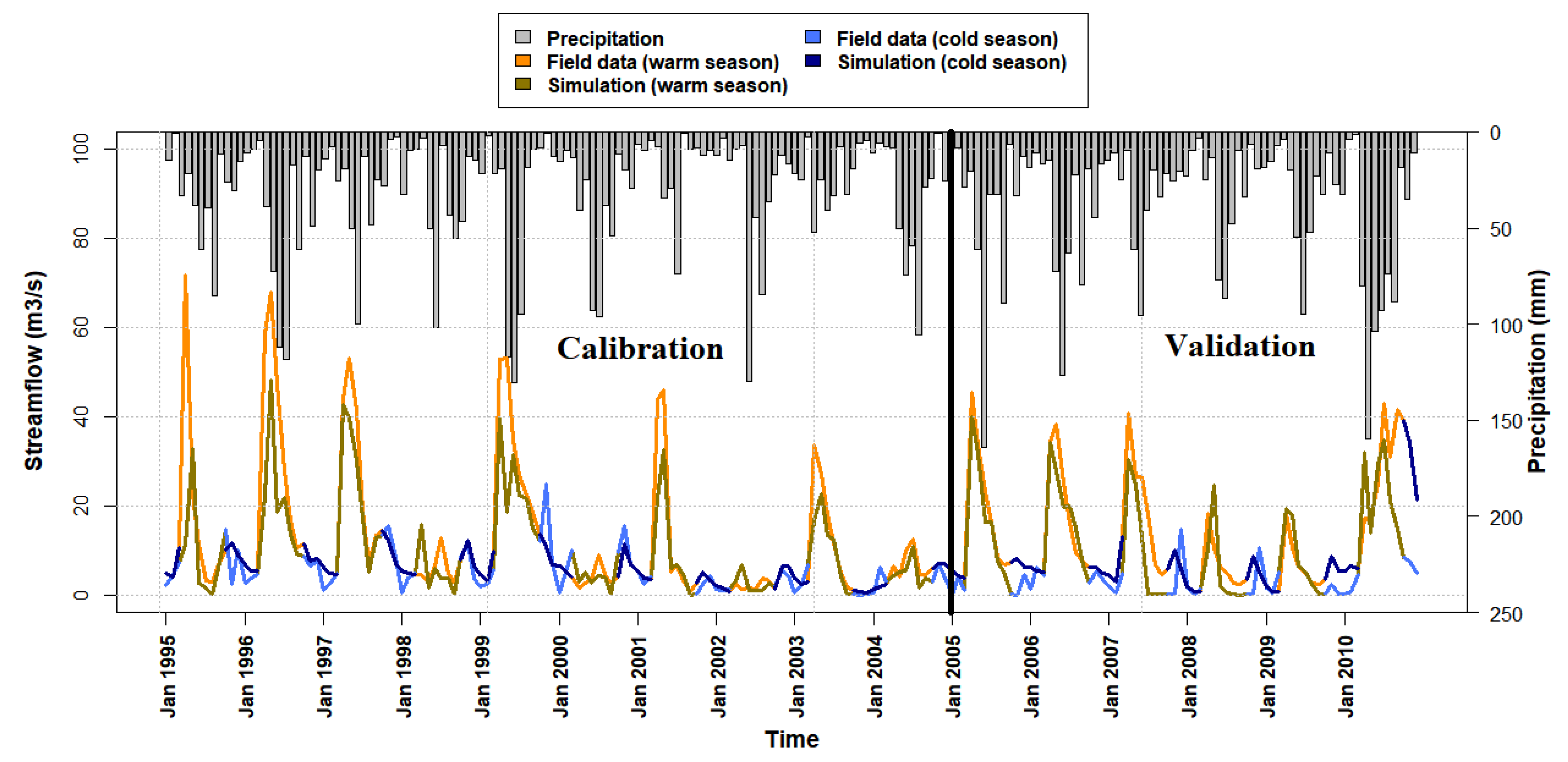
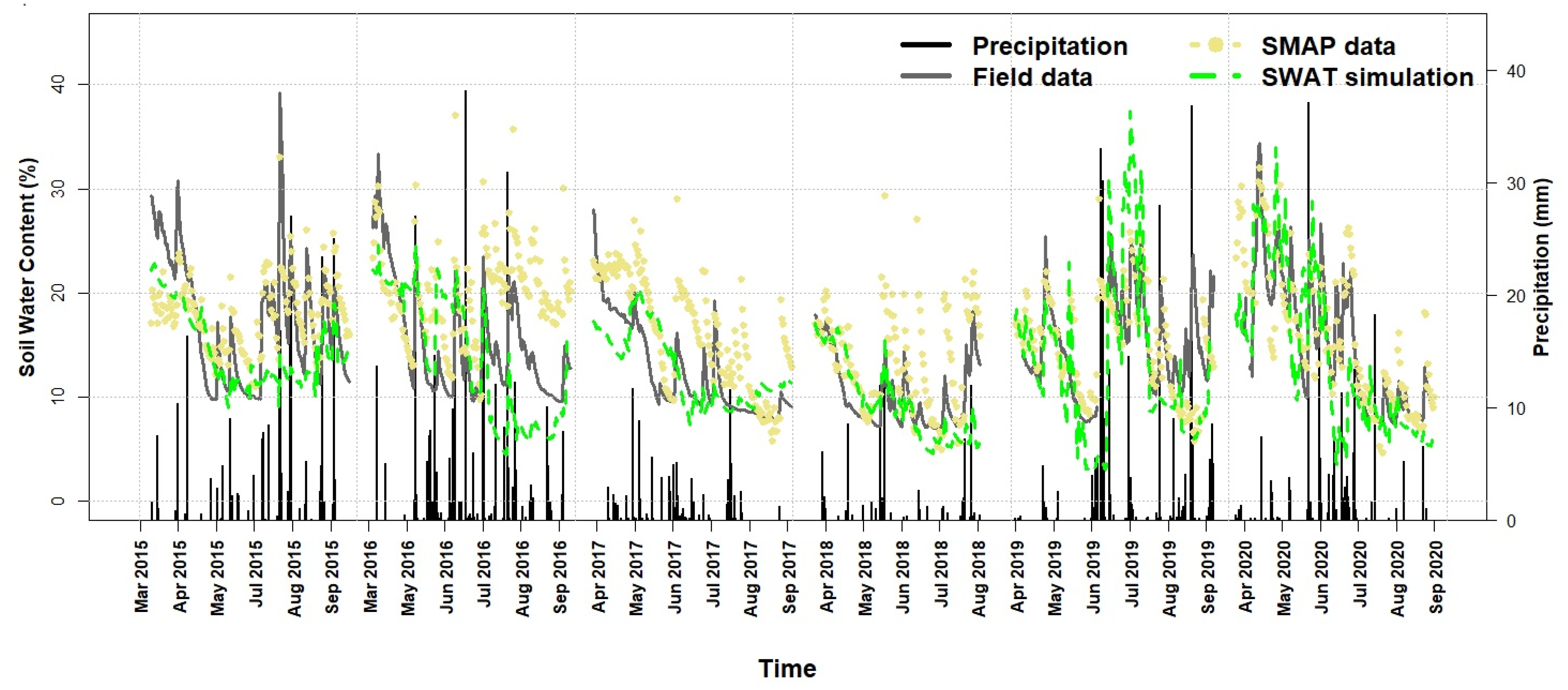
3. Results and Discussion

Table 2 shows the results of the sensitivity analysis. Results are rank ordered for the most sensitive (high t- values) and most significant (closer to zero for p-values) parameters affecting SWC out of a total of 30 inputs based on a batch of iterations. Among all input parameters, we selected 14 that heavily depend on observed streamflow and SWC. The data indicate that the base flow alpha factor (ALPHA_BF) has the most sensitivity among all parameters (p-value = 0). If the ALPHA_BF value is between 0.1 and 0.3, there is a slow recharge response in the region [13]. The optimal value of ALPHA_BF ranges between the values of 0.1 to 0.3. Previous research [32,33] had similar findings in southern Saskatchewan. The sensitivity of ALPHA_BF indicates the rapid infiltration and groundwater recharge in the semi-arid region. The high ALPHA_BF value shows a quick base flow recession and hence, this parameter plays a vital role in the low regional flow [34].
The next sensitive parameter is the groundwater re-evaporation coefficient (GW_REVAP) and effective hydraulic conductivity in the main channel alluvium (CH_K2). Southern Saskatchewan has mostly low slopes, and, thus, rainfall accumulates and infiltrates, leading to higher groundwater levels and, subsequently, to more base flow contribution to discharge. Moreover, during the dry summer months, there is relatively little runoff from the semi-arid landscape, and prairie streams are maintained by groundwater discharge.
Figure 3 compares observed and simulated streamflow during the calibration (1995–2004) and validation (2005–2010) periods. In both periods, the Nash–Sutcliffe efficiency (NSE) values (0.616 and 0.784, respectively) were more than 0.5, indicating satisfactory model performance. Similarly, higher values of R2 (0.82 and 0.8 for calibration and validation, respectively) confirmed the good correlation between observed and simulated streamflow. Moreover, results on a monthly timescale (Figure 3) were found to be similar between the calibration and validation periods. The SWAT model was able to simulate the relative contributions of precipitation and snowmelt to the streamflow to produce seasonal streamflow and lead time results [35]; although model performance was lower in the warm season than in the cold season. Peak flow in some months is underestimated, especially for April and May, while the model performs well for low and intermediate flow. These results are subject to uncertainties in the input data and structure of the model during snowmelt and runoff season. The accuracy and resolution of rainfall and temperature data significantly affected peak flow simulations, especially during snowmelt and runoff season [36]. Calibration in the SWAT model is based on a batch form whereby parameters are adjusted to corresponding input by modifying simulations with observations. Therefore, underestimation is due to an abrupt increase in streamflow during snowmelt months (April and May). Moreover, the validation of the batch form calibration is based on two assumptions, namely: the hydrological system is steady and devoid of abrupt changes and the calibrated model is robust enough [37], which is why the calibrated model does not perform well during snowmelt months.
Table 3 summarizes the correlations among daily SWAT and SMAP output and measured SWC based on three error metrics (i.e., RMSE, Bias, and R). The correlation coefficients between field measurement with SMAP and the SWAT product are 0.698 and 0.633, respectively. The RMSE values for SMAP and SWAT are 0.052 and 0.046, respectively.
Figure 4 depicts a time series of simulated SWC. The agreement of measurement data with SMAP and SWAT validates the ability of the SWAT to model SWC. The measurement data are a better fit with SMAP products compared with SWAT output. However, the measured range of SMAP data is higher than that of SWAT output and field measurement, while the range of SWAT SWC is lower than SMAP and field measurement. By using the brightness temperature and the radar backscatter, L4-SM data was found to be more prone to vegetation and surface roughness when this condition led to a reduced sensitivity to soil moisture in comparison to passive brightness temperature. Therefore, it makes a better soil moisture product than SWAT SWC. Another reason for the better performance is that L4_SM incorporates an algorithm that combines the information between the L-band Tb observations, the water and energy balance constraints captured in the land-surface model, and the information in the surface meteorological data. This function is derived from gauge-based precipitation observations and several atmospheric observations [38]. Various studies have emphasized the better performance of L4_SM products compared with ground measurements [26,39,40]. The good fit among all SWC products in the vegetation growing season (from May to September) reflects the SWAT model estimation of SWC based on the root system. Thus, the best correlation occurred when vegetation had reached its peak growth rate. This finding is consistent with the sensitivity analysis where the groundwater re-evaporation coefficient (GW_REVAP) shows high sensitivity. In this region, the saturated zone is not deep and deep-rooted plants can take up water directly from the water table. This is consistent with the reported observation [16,18,41], suggesting that correlations must be based on the growth period.
The direct relationship between rainfall and SWC was not symmetric. The SWC change in SWAT indicates a gradual increase and decrease, particularly after wetting and drying processes by rainfall and evapotranspiration. Soil texture in southern Saskatchewan is dominated by clay, which retains SWC, thereby resulting in slower rates of wetting and drying than in silt and sand. SWAT model and SMAP estimated SWC is noisy in the surface layer where there is the most interaction with the atmosphere [20,42,43].
Table 4 gives the results of monthly statistical analysis of SWC data based on Pearson correlation coefficient and bivariate correlation methods from 2015 to 2020 for the warm season (April to September). The highest r value occurred in July and June when mean r values in SWAT and SMAP were 0.87 to 0.84. Moreover, the mean value indicates that June has the highest r (0.96) value compared to other months. In contrast, the lowest values were in April and May (mean r values of 0.07 and 0.04, respectively) at the beginning and end of the growing season. The root system reaches its optimal extent after May. Most of the land cover consists of the annual crops and perennial pasture, which use SWC available in the top part of the soil profile [16]. Therefore, the highest correlation occurs when vegetation has reached its maximum growth rate. SWC is estimated in the SWAT model based on the actual root system (0–30 cm) and, thus, the best correlation between SWC and SMAP with field measurement was during the growing season.
Figure 5 gives the monthly comparison of SWC between SWAT, SMAP, and measurement data along with the difference of potential evapotranspiration and precipitation. The results indicate that the highest difference between rainfall and evapotranspiration was 130 mm in August 2017, while the mean SWC has the lowest value (12.4%, 14%, and 8.8% in field measurement, SMAP, and SWAT, respectively) in the same month.
While SWC is directly connected to ET, heterogeneity in daily PET-precipitation and SWC is due to small rainfalls of short duration (for high PET and low SWC). Two factors play a vital role in such cases. Firstly, evaporation from soil and leaf surfaces are sufficient to prevent wetting below the surface soil. Secondly, relatively heavy rainfall when potential evapotranspiration demand remains low and soil recharge become rapid [44,45,46,47]. In such cases, the lowest difference between rainfall and evapotranspiration (21.78 mm) was in May 2016. In contrast, the average SWC had high values (14.4%, 18.5%, and 18% in field measurement, SMAP, and SWAT, respectively) in this month.

4. Summary and Conclusions

The SWAT-CUP model was calibrated and validated by the SUFI-2 algorithm over the 1995–2004 and 2005–2010 periods, respectively. Sensitivity analysis was conducted to adjust the most sensitive input parameters in the ArcSWAT model that were then given more attention in the calibration process. The ArcSWAT model obtained good simulation results for the mean monthly river discharge of in southern Saskatchewan, with BIAS less than 10% and NSE and R higher than 0.8 in the region. Further results can be enhanced using model runs on daily weather and SWC data along with satellite SWC data over a more extended period. Therefore, the reliability of SWC derived from the SWAT model was tested by correlating SMAP and field measure data with SWAT output. The results indicate this correlation depends on the depth of the root zone and variability of local conditions so that July and June have the highest r-value when vegetation has reached its maximum growth rate. However, the local conditions and short intense precipitation events have an effective role in SWC fluctuations. Soil water content in the SWAT model can reasonably simulate the spatiotemporal variations and trend of regional SWC in shallow soil layers. Moreover, there is a strong correlation between SWC measurement and SMAP data. Level 4 in the SMAP mission product uses the brightness temperature and, thus, is more prone to the combined effects of vegetation and surface roughness when this condition leads to a reduced sensitivity to soil moisture in comparison to passive brightness temperature. Therefore, it could be a better SWC product than the performance of SWC in SWAT. Moreover, SWAT tended to overestimate SWC in the surface layer after rainfall events and snowmelt season in the cold region. This is because calibration in the SWAT model is based on batch form and the validation of the batch form calibration is according to the assumption that the hydrological system is a steady system without abrupt changes and the calibrated model is robust enough. Therefore, underestimation is found due to an abrupt increase in streamflow during snowmelt months (April and May).

Author Contributions

Data curation and analysis, M.Z.; Supervision, S.A. and D.S.; Writing—original draft, M.Z.; Writing—review & editing, S.A. and D.S. All authors have read and agreed to the published version of the manuscript.

Funding

Natural Science and Engineering Research Council of Canada.

Institutional Review Board Statement

Not applicable.

Informed Consent Statement

Not applicable.

Data Availability Statement

The authors can provide access to modeling data upon request.

Acknowledgments

The authors would like to thank the University of Regina for providing laboratory space.

Conflicts of Interest

The authors declare there is no conflict of interest.

References

  1. Hong, W.; Park, M.; Park, J.; Park, G.; Kim, S. The spatial and temporal correlation analysis between MODIS NDVI and SWAT predicted soil moisture during forest NDVI increasing and decreasing periods. KSCE J. Civ. Eng. 2010, 14, 931–939. [Google Scholar] [CrossRef]
  2. Uniyal, B.; Dietrich, J.; Vasilakos, C.; Tzoraki, O. Evaluation of SWAT simulated soil moisture at catchment scale by field measurements and Landsat derived indices. Agric. Water Manag. 2017, 193, 55–70. [Google Scholar] [CrossRef]
  3. Champagne, C.; Berg, A.; McNairn, H.; Drewitt, G.; Huffman, T. Evaluation of soil moisture extremes for agricultural productivity in the Canadian prairies. Agric. For. Meteorol. 2012, 165, 1–11. [Google Scholar] [CrossRef]
  4. McGinn, S.M.; Shepherd, A. Impact of climate change scenarios on the agroclimate of the Canadian prairies. Can. J. Soil Sci. 2003, 83, 623–630. [Google Scholar] [CrossRef]
  5. Akhter, A.; Azam, S. Flood-drought hazard assessment for a flat clayey deposit in the Canadian Prairies. J. Environ. Inform. Lett. 2019, 1, 8–19. [Google Scholar] [CrossRef]
  6. Saskatchewan Ministry of Agriculture. 2012. Available online: http://www.agriculture.gov.sk.ca/ (accessed on 28 August 2021).
  7. Pomeroy, J.; De Boer, D.; Martz, L. Hydrology and Water Resources of Saskatchewan; Report no. 1; Center for Hydrology: Saskatoon, SK, Canada, 2005. [Google Scholar]
  8. Bressiani, D.A.; Gassman, P.W.; Fernandes, J.G.; Garbossa, L.H.; Srinivasan, R.; Bonumá, N.B.; Mendiondo, E.M. A review of SWAT (Soil and Water Application Tool) applications in Brazil: Challenges and prospects. Int. J. Agric. Biol. Eng. 2015, 8, 9–35. [Google Scholar]
  9. Douglas-Mankin, K.R.; Srinivasan, R.; Arnold, J.G. Soil and Water Assessment Tool (SWAT) model: Current developments and applications. Trans. ASABE 2010, 53, 1423–1431. [Google Scholar] [CrossRef]
  10. Gassman, P.W.; Reyes, M.R.; Green, C.H.; Arnold, J.G. The Soil and Water Assessment Tool: Historical development, applications, and future research directions. Trans. ASABE 2007, 50, 1211–1240. [Google Scholar] [CrossRef] [Green Version]
  11. Krysanova, V.; White, M. Advances in water resources assessment with SWAT—An overview. Hydrol. Sci. J. 2015, 60, 771–783. [Google Scholar] [CrossRef] [Green Version]
  12. Tuppad, P.; Douglas-Mankin, K.R.; Lee, T.; Srinivasan, R.; Arnold, J. Soil and Water Assessment Tool (SWAT) hydrologic/water quality model: Extended capability and wider adoption. Am. Soc. Agric. Biol. Eng. 2011, 54, 1677–1684. [Google Scholar] [CrossRef]
  13. Arnold, J.G.; Moriasi, D.N.; Gassman, P.W.; Abbaspour, K.C.; White, M.J.; Srinivasan, R.; Santhi, C.; Harmel, R.D.; Van Griensven, A.; Van Liew, M.W.; et al. SWAT: Model use, calibration, and validation. Trans. ASABE 2012, 55, 1491–1508. [Google Scholar] [CrossRef]
  14. Mapfumo, E.; Chanasyk, D.S.; Willms, W.D. Simulating daily soil water under foothills fescue grazing with the Soil and Water Assessment Tool model (Alberta, Canada). Hydrol. Process. 2004, 18, 2787–2800. [Google Scholar] [CrossRef]
  15. Refsgaard, J.C.; Storm, B. MIKE-SHE. In Computer Models of Watershed Hydrology; Singh, V.J., Ed.; Water Resources Pub.: Englandwood, CO, USA, 1995; pp. 809–846. [Google Scholar]
  16. Narasimhan, B.; Srinivasan, R. Development and evaluation of Soil Moisture Deficit Index (SMDI) and Evapotranspiration Deficit Index (ETDI) for agricultural drought monitoring. Agric. For. Meteorol. 2005, 133, 69–88. [Google Scholar] [CrossRef]
  17. Park, J.Y.; Ahn, S.R.; Hwang, S.J.; Jang, C.H.; Park, G.A.; Kim, S.J. Evaluation of MODIS NDVI and LST for indicating soil moisture of forest areas based on SWAT modeling. Int. Soc. Pad. Water. Environ. Eng. 2014, 121, 77–88. [Google Scholar] [CrossRef]
  18. Havrylenko, S.B.; Bodoque, J.M.; Srinivasan, R.; Zucarelli, G.V.; Mercuri, P. Assessment of the soil water content in the Pampas region using SWAT. Catena 2016, 137, 298–309. [Google Scholar] [CrossRef]
  19. Nilawar, A.P.; Calderella, C.P.; Lakhankar, T.Y. Satellite soil moisture validation using hydrological SWAT model: A case study of Puerto Rico, USA. Hydrology 2017, 4, 45. [Google Scholar] [CrossRef] [Green Version]
  20. Rajib, A.; Merwade, V.; Kim, I.L.; Zhao, L.; Song, C.; Zhe, S. SWATShare—A web platform for collaborative research and education through online sharing, simulation and visualization of SWAT models. Environ. Model. Softw. 2016, 75, 498–512. [Google Scholar] [CrossRef] [Green Version]
  21. Azimi, S.; Dariane, A.; Modanesi, S.; Bauer-Marschallinger, B.; Bindlish, R.; Wagner, W.; Massari, C. Assimilation of Sentinel 1 and SMAP–based satellite soil moisture retrievals into SWAT hydrological model: The impact of satellite revisit time and product spatial resolution on flood simulations in small basins. J. Hydrol. 2020, 581, 1–16. [Google Scholar] [CrossRef]
  22. Breen, K.; James, S.; White, J.; Allan, P.; Arnold, J. A Hybrid Artificial Neural Network to Estimate Soil Moisture Using SWAT+ and SMAP Data, Mach. Learn. Knowl. Extr. 2020, 2, 283–306. [Google Scholar]
  23. Li, D.; Liang, Z.; Li, B.; Lei, X.; Zhou, Y. Multi-objective calibration of MIKE SHE with SMAP soil moisture datasets. Hydrol. Curr. Res. 2019, 50, 644–654. [Google Scholar] [CrossRef] [Green Version]
  24. Yi, L.; Zhang, Q.; Li, X. Assessing hydrological modelling driven by different precipitation datasets via the SMAP soil moisture product and gauged streamflow data. Remote Sens. 2018, 10, 1872. [Google Scholar] [CrossRef] [Green Version]
  25. Tavakol, A.; Rahmani, V.; Quiring, S.M.; Kumar, S.V. Evaluation analysis of NASA SMAP L3 and L4 and SPoRT-LIS soil moisture data in the United States. Remote Sens. Environ. 2019, 229, 234–246. [Google Scholar] [CrossRef]
  26. Reichle, R.H.; de Lannoy, G.; Koster, R.D.; Crow, W.T.; Kimball, J.S. Assessment of the SMAP Level-4 Surface and Root-Zone Soil Moisture Product Using In Situ Measurements. J. Hydrometeorol. 2017, 18, 2621–2645. [Google Scholar] [CrossRef]
  27. Abbaspour, K.C. SWAT-CUP: SWAT Calibration and Uncertainty Programs—A User Manual; Open File Rep.; Eawag, Swiss Federal Institute of Aquatic Science and Technology: Dübendorf, Switzerland, 2015; 100p. [Google Scholar]
  28. Nash, J.E.; Sutcliffe, J.V. River flow forecasting through conceptual models: Part I—A discussion of principles. J. Hydrol. 1970, 10, 282–290. [Google Scholar] [CrossRef]
  29. Moriasi, D.N.; Arnold, J.G.; Van Liew, M.W.; Binger, R.L.; Harmel, R.D.; Veith, T. Model evaluation guidelines for systematic quantification of accuracy in watershed simulations. Trans. ASABE 2007, 50, 885–900. [Google Scholar] [CrossRef]
  30. Legates, D.R.; McCabe, G.J. Evaluating the use of “goodness-of-fit” measures in hydrologic and hydroclimatic model validation. Water Resour. Res. 1999, 35, 233–241. [Google Scholar] [CrossRef]
  31. Musyoka, F.K.; Strauss, P.; Zhao, G.; Srinivasan, R.; Klik, A. Multi-Step calibration approach for SWAT model using soil moisture and crop yields in a small agricultural catchment. Water 2021, 13, 2238. [Google Scholar] [CrossRef]
  32. Perez-Valdivia, C.; Cade, B.; McMartin, D. Hydrological modeling of the pipestone creek watershed using the Soil Water Assessment Tool (SWAT): Assessing impacts of wetland drainage on hydrology. J. Hydrol. 2017, 14, 109–129. [Google Scholar] [CrossRef]
  33. Mekonnen, B.; Mazurek, K.; Putz, G. Incorporating landscape depression heterogeneity into the Soil and Water Assessment Tool (SWAT) using a probability distribution. Hydrol. Process. 2016, 30, 2373–2389. [Google Scholar] [CrossRef]
  34. Zhao, F.; Wu, Y.; Qiu, L.; Sun, Y.; Sun, L.; Li, Q.; Niu, J.; Wang, G. Parameter uncertainty analysis of the SWAT model in a Mountain-Loess Transitional watershed on the Chinese Loess Plateau. Water 2018, 10, 690. [Google Scholar] [CrossRef] [Green Version]
  35. Zheng, X.; Wang, Q.; Zhou, L.; Sun, Q.; Li, Q. Predictive Contributions of Snowmelt and Rainfall to Streamflow Variations in the Western United States. Adv. Meteorol. 2018, 2018, 1–15. [Google Scholar] [CrossRef]
  36. Due, X.; Goss, G.; Faramarzi, M. Impacts of Hydrological Processes on Stream Temperature in a Cold Region Watershed Based on the SWAT Equilibrium Temperature Model. Water 2020, 12, 1112. [Google Scholar] [CrossRef] [Green Version]
  37. Sun, N.; Yearsley, J.; Baptiste, M.; Cao, Q.; Lettenmaier, D.P.; Nijssen, B. A spatial distributed model for assessment of the effects of changing land use and climate on urban stream quality. Hydrol. Process. 2016, 30, 4779–4798. [Google Scholar] [CrossRef]
  38. Reichle, R.H.; Liu, Q.; Koster, R.D.; Crow, W.T.; De Lannoy, G.J.M.; Kimball, J.S.; Ardizzone, J.V.; Bosch, D.; Colliander, A.; Cosh, M.; et al. Version 4 of the SMAP level-4 soil moisture algorithm and data product. J. Adv. Model. Earth Syst. 2019, 11, 3106–3130. [Google Scholar] [CrossRef] [Green Version]
  39. Crow, W.T.; Chen, F.; Reichle, R.H.; Xia, Y. Diagnosing bias in modeled soil moisture/runoff coefficient correlation using the SMAP Level 4 soil moisture product. Water Resour. Res. 2019, 55, 7010–7026. [Google Scholar] [CrossRef]
  40. Dong, J.; Crow, W.T.; Reichle, R.H.; Liu, Q.; Lei, F.; Cosh, M. A global assessment of added value in the SMAP Level-4 Soil Moisture product relative to its baseline land surface model. Geophys. Res. Lett. 2019, 46, 6604–6613. [Google Scholar] [CrossRef]
  41. Richard, J.; Madramootoo, C.; Trotman, A. Application of the Standardized Precipitation Index and Normalized Difference Vegetation Index for Evaluation of Irrigation Demands at Three Sites in Jamaica. J. Irrig. Drain. Eng. 2013, 139, 922–932. [Google Scholar] [CrossRef]
  42. Milzow, C.; Krogh, P.E.; Bauer-Gottwein, P. Combining satellite radar altimetry, SAR surface soil moisture and GRACE total storage changes for hydrological model calibration in a large poorly gauged catchment. Hydrol. Earth Syst. Sci. 2016, 15, 1729–1743. [Google Scholar] [CrossRef] [Green Version]
  43. Wanders, N.; Bierkens, M.F.P.; De Jong, S.M.; de Roo, A.; Karssenberg, D. The benefits of using remotely sensed soilmoisture in parameter identification of large-scale hydrologicalmodels. Water Resour. Res. 2014, 50, 6874–6891. [Google Scholar] [CrossRef] [Green Version]
  44. Liu, X.; Luo, Y.; Zhang, D.; Zhang, M.; Liu, C. Recent changes in pan-evaporation dynamics in China. Geophys. Res. Lett. 2011, 38, 1–4. [Google Scholar] [CrossRef] [Green Version]
  45. Purdy, A.J.; Fisher, J.B.; Goulden, M.L.; Colliander, A.; Halverson, G.; Tu, K.; Famiglietti, J.S. SMAP soil moisture improves global evapotranspiration. Remote Sens. Environ. 2018, 219, 1–14. [Google Scholar] [CrossRef]
  46. Verstraeten, W.; Veroustraete, F.; Feyen, J. Assessment of evapotranspi-ration and soil moisture content across different scales of observation. Sensors 2008, 8, 70–117. [Google Scholar] [CrossRef] [PubMed] [Green Version]
  47. Wang, T.; Franz, T.E. Field observations of regional controls of soil hydraulic properties on soil moisture spatial variability in different climate zones. Vadose Zone J. 2015, 14, 1–8. [Google Scholar] [CrossRef]
Figure 1. Flow chart of the modeling program.
Water 14 00249 g001
Figure 2. Map of the study region.
Water 14 00249 g002
Figure 3. Simulated and observed stream flows and precipitation.
Water 14 00249 g003
Figure 4. Temporal comparison of soil water content.
Water 14 00249 g004
Figure 5. Monthly comparison soil water content between SWAT, SMAP, and field data.
Water 14 00249 g005
Table 1. Input data used in SWAT model.
Data Type DescriptionInformation Source
Digital Elevation ModelWatershed delineationRaster, 20 m-resolutionhttp://geogratis.gc.ca
accessed on 28 September 2020
Land use Land-use classificationRaster, 30 m-resolutionhttp://geogratis.gc.ca
accessed on 30 September 2020
Soil typeSoil properties Vector http://www.agr.gc.ca
accessed on 2 October 2020
Weather Precipitation and temperatureDaily https://weather.gc.ca
accessed on 15 November 2020
Streamflow Calibration and validation modelDaily https://wateroffice.ec.gc.ca
accessed on 16 December 2020
Table 2. Parameters used for calibration with optimum values.
ParameterDescriptionTypeInitial RangeOptimal Valuep-Valuet-StateRank
ALPHA_BFBase flow alpha factorv0.0–1.00.1–0.2410.000−36.261
GW_REVAPGround water re-evaporation coefficientv−0.2–0.20.1–0.170.00016.892
CH_K2Effective hydraulic conductivity in main channel alluvium (mm/h)v0.0–500154–6420.00114.733
CN2Curve number at moisture condition IIr−0.2–0.2−0.13–0.0380.00813.214
GWQMNThreshold depth of water in the shallow aquifer required for return flow (mm)r0.0–0.20.64–1.940.07410.95
SOL_ALBMoist soil albedor0–0.250.08–0.1390.08−10.76
ESCOSoil evaporation compensation factorv0.0–1.00.241–0.8320.3549.267
CH_N2Manning’s ‘‘n’’ value for the channelv0.0–0.30.09–0.2720.382−8.748
GW_DELAYGroundwater delay (days)v0–500181–2720.533−0.6239
SOL_BDSaturated hydraulic conductivity of first layerr−0.1–1.0−0.005–0.1830.5510.59610
SURLAGSurface runoff lag coefficient (day)v0.0–242.68–23.040.7870.27211
SOL_AWCSoil water available capacityr−0.1–1.0−0.061–0.3570.7960.25712
SOL_KSaturated hydraulic conductivity (mm/h)r−0.1–1.0−0.011–0.0270.803−0.24813
SOL_ZDepth from the soil surface to layer bottom r−0.1–1.0−0.03–0.0210.842−0.19814
Table 3. Daily calibration of SWAT model with field measurement data and SMAP.
Data RMSEBiasRp-ValueN
MeasurementSWAT0.0460.0120.6330.000703
SMAP0.052−0.0350.6980.000703
SWATSMAP0.106−0.0960.3730.000703
Table 4. Monthly statistical analysis between SWC databases.
Statistical IndicesData AprilMayJuneJulyAugustSeptember
RMeasurementSWAT−0.0550.0630.7250.8640.60.605
SMAP0.0910.020.9660.8770.7820.762
SWATSMAP−0.0360.1070.7480.1520.3060.247
Publisher’s Note: MDPI stays neutral with regard to jurisdictional claims in published maps and institutional affiliations.

