Article

Application of Artificial Neural Networks for Mangrove Mapping Using Multi-Temporal and Multi-Source Remote Sensing Imagery

1
Department of Photogrammetry and Remote Sensing, Faculty of Geodesy and Geomatics Engineering, K. N. Toosi University of Technology, Tehran 19967-15433, Iran
2
Wood Environment & Infrastructure Solutions, Ottawa, ON K2E 7L5, Canada
3
Department of Technology and Society, Faculty of Engineering, Lund University, P.O. Box 118, 22100 Lund, Sweden
*
Author to whom correspondence should be addressed.
Water 2022, 14(2), 244; https://doi.org/10.3390/w14020244
Submission received: 20 November 2021 / Revised: 22 December 2021 / Accepted: 12 January 2022 / Published: 15 January 2022
(This article belongs to the Special Issue Mapping and Monitoring of Wetlands)

Abstract

:
Mangroves, as unique coastal wetlands with numerous benefits, are endangered mainly due to the coupled effects of anthropogenic activities and climate change. Therefore, acquiring reliable and up-to-date information about these ecosystems is vital for their conservation and sustainable blue carbon development. In this regard, the joint use of remote sensing data and machine learning algorithms can assist in producing accurate mangrove ecosystem maps. This study investigated the potential of artificial neural networks (ANNs) with different topologies and specifications for mangrove classification in Iran. To this end, multi-temporal synthetic aperture radar (SAR) and multi-spectral remote sensing data from Sentinel-1 and Sentinel-2 were processed in the Google Earth Engine (GEE) cloud computing platform. Afterward, the ANN topologies and specifications considering the number of layers and neurons, learning algorithm, type of activation function, and learning rate were examined for mangrove ecosystem mapping. The results indicated that an ANN model with four hidden layers, 36 neurons in each layer, adaptive moment estimation (Adam) learning algorithm, rectified linear unit (Relu) activation function, and the learning rate of 0.001 produced the most accurate mangrove ecosystem map (F-score = 0.97). Further analysis revealed that although ANN models were subjected to accuracy decline when a limited number of training samples were used, they still resulted in satisfactory results. Additionally, it was observed that ANN models had a high resistance when training samples included wrong labels, and only the ANN model with the Adam learning algorithm produced an accurate mangrove ecosystem map when no data standardization was performed. Moreover, further investigations showed the higher potential of multi-temporal and multi-source remote sensing data compared to single-source and mono-temporal (e.g., single season) for accurate mangrove ecosystem mapping. Overall, the high potential of the proposed method, along with utilizing open-access satellite images and big-geo data processing platforms (i.e., GEE, Google Colab, and scikit-learn), made the proposed approach efficient and applicable over other study areas for all interested users.

1. Introduction

Mangrove ecosystems are among the most productive ecosystems that exist along coastal areas in tropical and sub-tropical regions. These ecosystems provide unique ecological and environmental benefits including coastal protection (i.e., against floods and wave attenuation) [1,2], carbon sequestration [3,4], pollution and waste abatement [5,6], and pharmaceutical production [7,8]. Additionally, mangrove ecosystems are important habitats for various fauna, providing valuable food services for shrimp farming and fishery [9,10]. However, mangrove loss (i.e., in species and extent) due to the fact of anthropogenic activities, catastrophic natural hazards in coastal areas, and climate change continued in recent decades has led to severe environmental degradation [11,12,13,14]. Accordingly, it is a global, regional, and local concern to accurately map these valuable ecosystems to prevent their loss and establish effective practices for their sustainable management.
In the current era, the advancement of remote sensing technology has created an unprecedented opportunity to study various natural resources such as mangrove communities [15,16,17,18,19,20]. In particular, remote sensing systems provide frequent and accurate data sets over mangrove communities with spatial consistency and synoptic views. These capabilities make remote sensing an appealing choice for mangrove studies compared to conventional approaches that rely on in situ data collection. This is rooted in the fact that conventional practices are time consuming, resource intensive, and, on some occasions, infeasible (i.e., due to the limited access and harsh environment of mangrove communities or large-scale studies) [21,22].
Remote sensing data sets have different characteristics in terms of electromagnetic spectrum domains, spatial resolutions, temporal resolutions, and radiometric resolutions. In particular, multi-spectral, synthetic aperture radar (SAR), light detection and ranging (LiDAR), and hyperspectral data are common remote sensing resources that have been employed either individually or in conjunction for mangrove studies [23,24,25,26,27,28]. For instance, Ashiagbor et al. [29] examined the capability of the Sentinel-1 SAR data to obtain information about mangroves in the Keta Lagoon Complex Ramsar Site (KLCRS) to support sustainable conservation and restoration. Likewise, Bindu et al. [30] employed multi-spectral images, in situ data, and allometric equations [31] to derive the above-ground biomass of mangroves and then converted the estimated values to carbon content. Moreover, Hu et al. [32] incorporated LiDAR, multi-spectral, topographical, and climate data to estimate the above-ground biomass density of mangrove communities. In another study, Lucas et al. [33] integrated time-series multi-spectral and SAR data to estimate mangroves’ age in Matang Mangrove Forest Reserve (MMFR), Malaysia. Later, interferometric SAR data were combined with very high-resolution stereo images to estimate the canopy height of mangroves [33].
Along with remote sensing data, machine learning algorithms have been extensively employed to exploit the full potential of these data for automated mapping of mangroves. In this respect, different machine learning algorithms, including maximum likelihood [34], support vector machine (SVM) [35], random forest (RF) [36,37], K nearest neighbor (KNN) [38], classification and regression trees (CART) [39], and artificial neural networks (ANNs) [40] have been utilized. For example, Parida and Kumar [35] implemented an SVM algorithm to map mangrove extent between 2009 and 2019 using Landsat-5 and Sentinel-2 data sets. Their results indicated an increase in the spatial extent of mangroves in the Odisha coast, which were mainly associated with plantation, awareness, restoration, and management. Moreover, Behera et al. [37] applied an RF algorithm for mangrove mapping in Bhitarkanika Wildlife Sanctuary, India. To this end, red-edge spectral bands and chlorophyll absorption information of AVIRIS-NG and Sentinel-2 images were employed, and the results indicated the preeminence of Sentinel-2 images for this task. Likewise, Zhang et al. [41] used multi-temporal Landsat-5 and digital elevation model (DEM) data to map mangrove forests based on a decision tree algorithm. It was reported that employing multi-temporal data can efficiently enhance the classification results by reducing the tidal effect, and the decision tree approach was superior to conventional statistical classifiers. In another study, Bihamta Toosi et al. [42] compared the performances of four machine learning algorithms (i.e., linear SVM, radial SVM, RF, and regularization in discriminant analysis) for mangrove classification and change detection using Landsat archives. The k-fold cross-section validation step was executed, and it was reported that the RF algorithm achieved the best performance.
Previous studies have acknowledged the benefits of multi-source remote sensing data and different machine learning algorithms for mangrove classification [41,43,44,45,46]. Meanwhile, few studies have been conducted to generate mangrove maps using multi-spectral data and the ANN algorithm [40,47,48,49], and its practicability is underreported [40]. Nevertheless, the applicability of the ANN algorithm for mangrove ecosystem mapping using multi-temporal and multi-source remote sensing data has not been comprehensively explored.
Notwithstanding the foregoing, this study aimed to investigate the potential of combining the ANN algorithm and multi-source (i.e., multi-spectral and SAR) remote sensing data for mangrove ecosystem mapping. In this regard, the ANN algorithms with different topologies and specifications were implemented for mangrove ecosystem mapping. In particular, the effects of the number of layers and neurons, learning algorithms, type of activation functions, and learning rates for small-to-medium-sized ANN models were investigated. Subsequently, several other analyses were conducted to explore the impact of data transformation/standardization, a limited number of training samples, noise labels, as well as multi-temporal and multi-source remote sensing data sets on the classification accuracy using the ANN algorithm.

2. Study Area and Data Sets
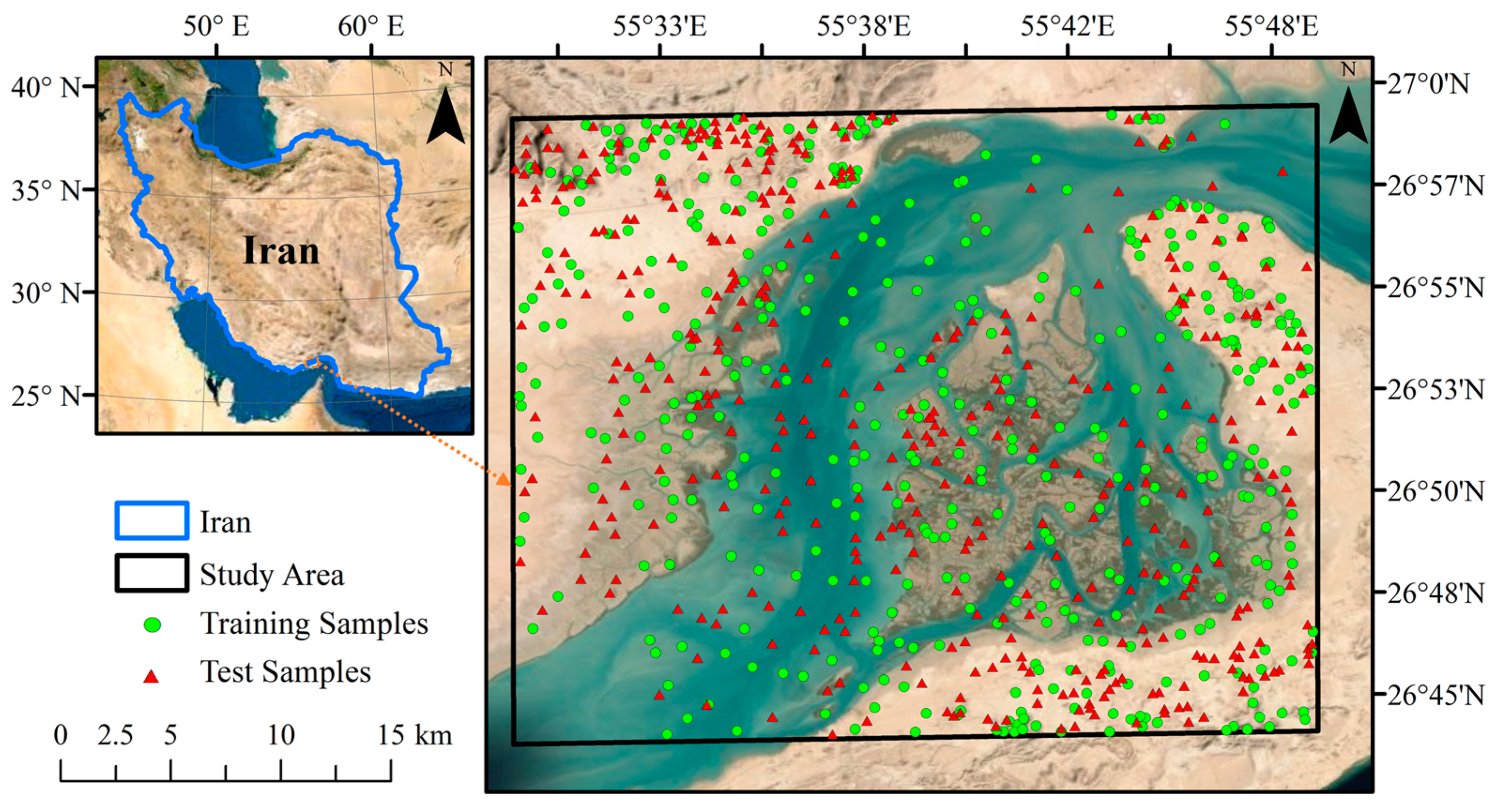
2.1. Study Area

The study was conducted over the Hara protected area, located between Khamir port and northwest estuaries of Qeshm Island at the latitudes and longitudes of 26°43′–26°59′ N and 55°28′–55°48′ E, respectively (see Figure 1). It is the largest mangrove community in the Persian Gulf and Oman Sea, with an area of over 850 km2 [50,51]. The Hara protected area has been officially registered as one of the biosphere reserves under the Ramsar Convention and included in UNESCO’s Man and Biosphere Program convention list [52]. This area includes vast intertidal zones and grooved tidal channels with considerable semi-diurnal tidal fluctuations with the minimum and maximum ranges of 0.3 and 4.6 m, respectively [53]. This suggests considering the tidal effect for accurate mangrove studies using multi-temporal imagery. Particularly, gray (Avicennia marina) and red (Rhizophora mucronata) mangrove species exist in the Persian Gulf (e.g., gray and red mangroves), and the gray mangrove (i.e., Avicennia marina, which belongs to the Acanthaceae family) is the dominant mangrove species in the Hara protected area [42,54]. This mangrove species cultivate in sediments with low-oxygen and high-salinity concentrations and are made of light gray bark and thick, glossy, bright green leaves [8,42]. This region has been impacted by anthropogenic practices of local and regional communities including leaf-cutting, fishing, boat journeys for tourism, oil leakage, and petrochemical industries [55,56,57]. Accordingly, developing efficient approaches is vital to obtain reliable information for the sustainable management of such valuable natural resources.

2.2. Reference Samples

Reference samples are required to support the training phase of a supervised classification algorithm and to evaluate its performance. In this study, reference samples were collected through visual interpretation of very high-resolution satellite images in Google Earth and ArcMap, which were captured in 2020. Additionally, the latest version of the global mangrove extent map [58] and the global distribution of tidal flat map [59] were also employed. To this end, these maps were overlaid on very high-resolution satellite images to identify suitable locations for collecting reference samples of the associate classes. This permitted selecting proper locations with higher confidence. In the first step, homogenous sites were considered to collect reference samples to avoid selecting mixed pixels as reference samples. In total, eight classes of land cover with appropriate spatial distribution (i.e., having suitable representativeness of reference samples over the study area) were initially collected (see Figure 1). Later, these samples were randomly divided into two independent sets of training and test samples. To this end, two criteria of size and number were considered. The random splitting approach of reference samples into two independent sets (i.e., training and test) would lead to low bias in the performance of the final classification results [60]. This step was implemented in the polygon unit, ensuring training and test samples with no spatial autocorrelation (i.e., spatially disjoint). This is because splitting reference samples into the pixel unit may lead to the leak of information (i.e., selection of training and test samples from a single polygon), affecting the evaluation step of the classification task and decreasing the generality of the classifier [61]. Afterward, several polygons were added to the mangrove test samples, selected from mangroves from narrow patches and sparse areas to better investigate the classification performance for the Mangrove class. This was because several parts of the study area included mangrove patches with narrow and fragmented conditions. Meanwhile, due to the importance of mangrove delineation, this practice could assure the robustness of the proposed method for the accurate mapping of mangroves located along the tidal zones. Table 1 summarizes the number and area of training and test samples. In total, 824 reference polygons were collected, 144.17 and 160.1 ha of which belonged to the training and test samples, respectively. The Barren class had a higher number of reference samples due to the fact of its higher diversity (i.e., surface variation in structure and color) and distribution in the study area. In contrast, the Vegetation class (e.g., croplands and inland forests/trees) had the lowest number of reference samples due to the fact of its scarcity in the region.

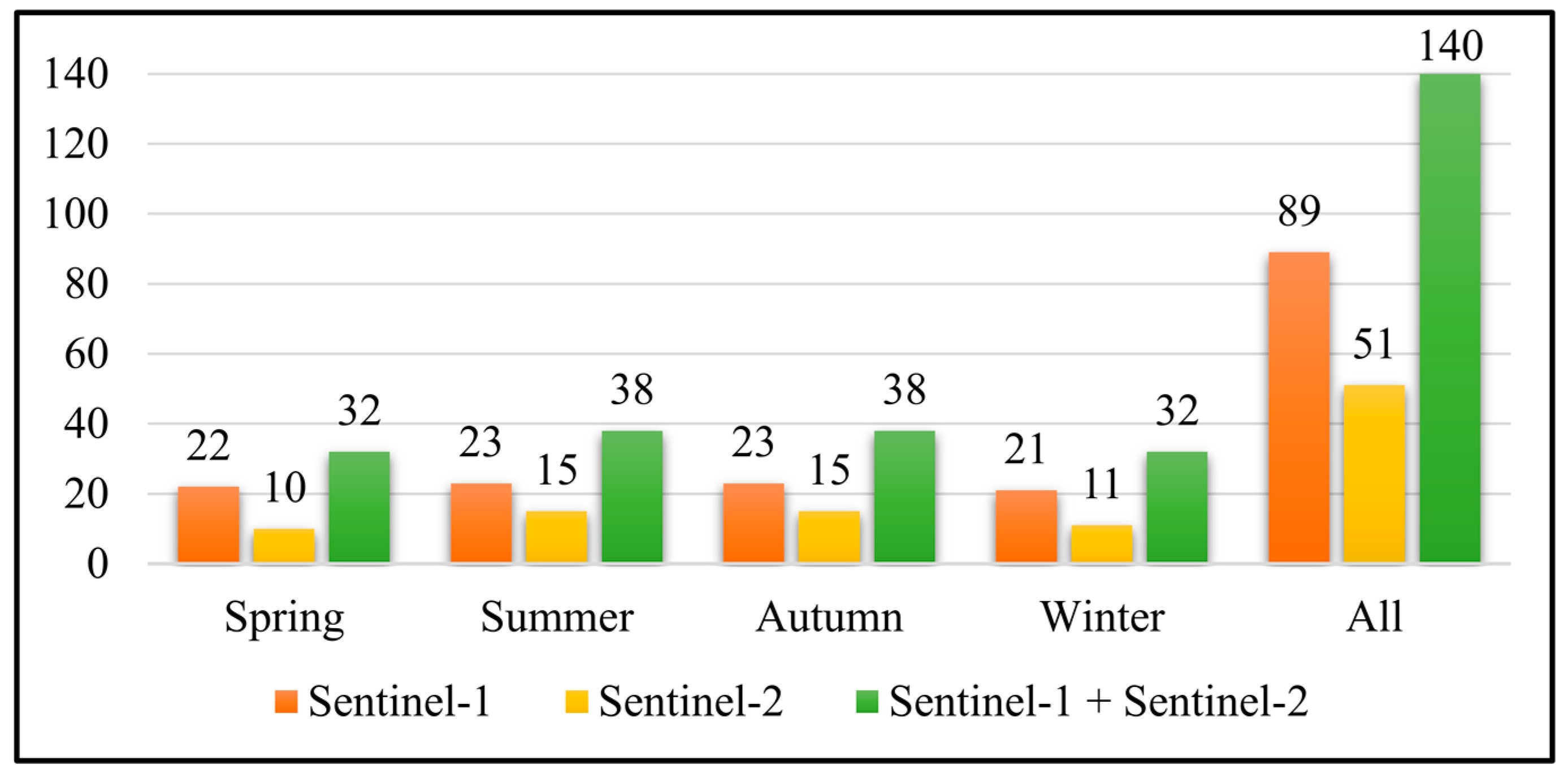
2.3. Satellite Images

This study employed a combination of multi-temporal Sentinel-1 and Sentinel-2 satellite images, which were available in Google Earth Engine (GEE). Sentinel-1 and Sentinel-2 are two European satellites developed by the joint cooperation of the European Space Agency (ESA) and European Commission initiative Copernicus [62].
GEE is a cloud computing platform that hosts petabytes of open-source geospatial data sets and allows for processing of a massive volume of data for various earth science tasks [63,64]. The synergistic use of SAR and optical data provides complementary information regarding the physical and spectral characteristics of existing land covers and leads to better discrimination, thus enhancing the classification results [65,66,67,68]. Furthermore, the utility of multi-temporal satellite images reduces the tidal effects and water level fluctuations in mangrove communities and, consequently, improves the reliability of the classification results [22].
Sentinel-1 captures all-weather C-band SAR data in dual-polarization with a 6 day revisit time. This sensor provides SAR data in three modes: Stripmap, Interferometric Wide Swath (IW), and Extra Wide Swath [69]. In this study, Ground Range Detected (GRD) Sentinel-1 images from the IW mode in ascending and descending orbits with a spatial resolution of 10 m were used. Overall, 89 Sentinel-1 scenes in both polarizations of VH (vertical transmittance and horizontal receiving) and VV (vertical transmittance and vertical receiving), acquired from 1 January 2020 to 1 January 2021 (i.e., whole scenes in 2020), were processed in this study (see Figure 2).
Sentinel-2 carries the MultiSpectral Instrument (MSI) sensor that allows for recording the Earth’s surface radiation in 13 spectral bands ranging from visible to shortwave infrared regions of the electromagnetic spectrum. The MSI captures spectral bands in the spatial resolutions of 10, 20, and 60 m. In this study, only spectral bands with the highest spatial resolution (i.e., blue, green, red, and near-infrared (NIR)) were utilized. This was because it was proved that higher resolution images enhance the mangrove ecosystem classification results [70]. This is rooted in the fact that satellite imagery with a higher spatial resolution has an advanced capability to delineate mangrove patches with narrow shapes and small areas [70]. In total, 51 available Sentinel-2 scenes in GEE with a cloud cover lower than or equal to (≤)5%, acquired between 1 January 2020 and 1 January 2021 (i.e., whole scenes in 2020), were employed in the classification (see Figure 2).

3. Methodology

The proposed methodology has three main steps, which are explained in the following three subsections. The satellite image preprocessing is initially described, followed by detailed explanations of the ANN models and classification procedure. Finally, the accuracy assessment of the classification results is discussed.

3.1. Satellite Images Preprocessing

In this study, time-series Sentinel-1 GRD products were collected from GEE. The GEE developers applied five common preprocessing steps to all GRD scenes, making them suitable as ready-to-use data for many applications [71]. In this regard, the following five preprocessing steps were first implemented, the detailed information of which is available by the GEE developers in [72]: (1) orbit file correction, (2) GRD border noise removal, (3) thermal noise removal, (4) radiometric calibration, and (5) terrain correction. Afterwards, a speckle filtering step was applied to all Sentinel-1 scenes. To this end, a mono-temporal improved Lee sigma despeckling algorithm with a kernel size of 5 × 5 was implemented to reduce the undesirable speckle effect, enhancing pixel-based classification results [73,74]. Finally, all the preprocessed Sentinel-1 scenes were categorized based on acquisition seasons, and a mean reducer function was applied to aggregate Sentinel-1 images and to create seasonal SAR features. For instance, all Sentinel-1 scenes within spring included 44 features (22 VV + 22 VH), and the mean reducer function was applied to generate only two features of VV and VH for the spring season. It is worth noting that the implemented aggregation approach would decrease the negative effects of image acquisition conditions and also reduce the volume of the input data and speckle noise effect [46,75].
Sentinel-2 top of atmosphere (TOA) reflectance data were collected for this study. Similar to Sentinel-1, Sentinel-2 scenes were subjected to initial preprocessing steps in which orthorectification and radiometric calibration were performed [76]. Later, a cloud filtering step was considered to avoid the negative effect of clouds in optical images and, thus, only Sentinel-2 scenes with less than or equal to (≤)5% cloud cover were included for further steps. Subsequently, a median reducer was applied to all Sentinel-2 images in each season, and seasonal optical features (i.e., four bands in each season) were generated. This allowed for cloud-free and pure seasonal data sets to be generated with no noise and very dark/bright pixels [68,77].
In summary, the final satellite data set contained eight SAR and 16 optical features, which were applied to the ANN algorithm. It is well accredited that the quality of the classification tasks directly relies on the input features. As such, incorporating multi-source (i.e., SAR + optical) data increases the discriminative capability of the classifier [65,66,67,68]. Moreover, time-series satellite data can manifest the water level fluctuations in estuaries such as mangrove ecosystems [22]. Consequently, seasonal data sets can mitigate the tidal effects in the study area and allow for the production of cloud-free mosaics. Finally, all input features were transformed using the standard scaler approach (i.e., removing the mean and scaling to unit variance).

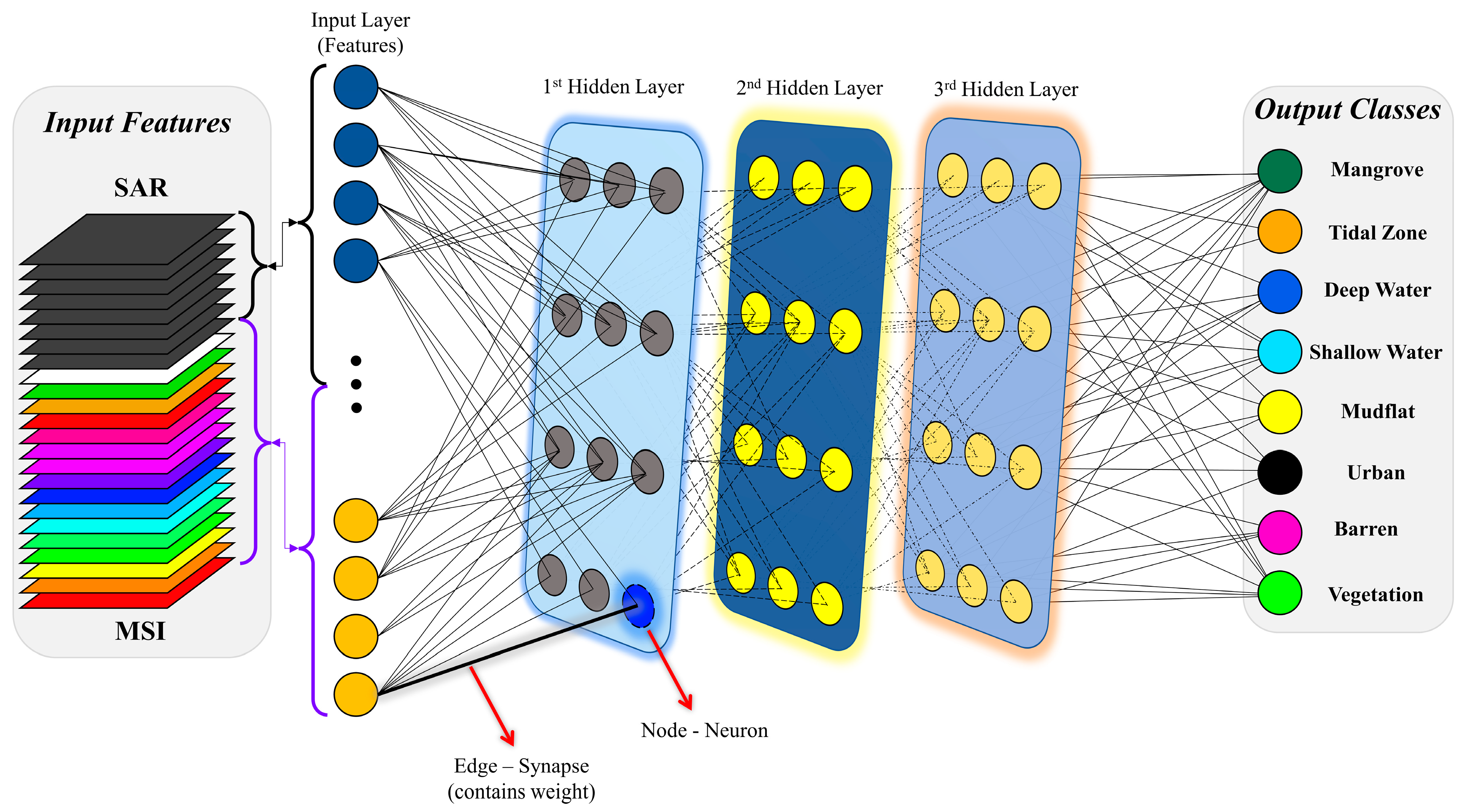
3.2. ANN Models and Classification

ANN is among the supervised machine learning algorithms inspired by the biological neurons system that emulates the human brain’s nervous recognition system [78]. ANNs are interconnected neurons that attempt to simulate neural processing and have high capabilities in nonlinear classification tasks [79,80].
Various types of ANN models exist of which the feedforward multi-layer perceptron (MLP) is the most common and practical model for classification and regression tasks [80,81,82]. The MLP models (hereafter called ANN) include input, hidden, and output layers in which a number of neurons (or nodes) and connections (or edges) exits. The data are transferred from the input layer to the output layer through these neurons and connections (see Figure 3). At the initial stage, the weight value of each connection is randomly assigned, and, later, the differences between the actual target classes/values and predicted classes/values (i.e., by the ANN model) are computed. This leads to weight values refinement through a backpropagation algorithm in an iterative manner [83]. The backpropagation algorithms calculate the gradient of the loss function and update the weight values for the next iteration [83]. This procedure continues until the ANN model is adequately trained, considering the satisfaction of the loss function.
Generally, four parameters are required to explicitly determine the architecture of an ANN model [80,84]: (1) number of layers, (2) number of neurons, (3) learning algorithm, and (4) type of activation function. These parameters directly influence the classification results of an ANN model and, hence, should be carefully determined to ensure achievement of the best possible accuracy.
In this study, different ANN topologies and specifications were implemented to examine the capability of ANN models for mangrove ecosystem mapping. To this end, the open-source scikit-learn package was used within the Google Colab platform so that other interested users could freely implement the analyses. In this regard, a grid search analysis was first performed to find the best number of layers (ranging between one and five layer(s)) and neurons (ranging between six and 36 neurons) using three different learning algorithms. This resulted in the investigation of 240 models. Three different learning algorithms were the adaptive moment estimation (Adam) [85], stochastic gradient descent (SGD) [86], and limited memory Broyden–Fletcher–Goldfarb–Shanno (LBFGS) [87]. Subsequently, the effect of the type of activation function was explored with the best topologies for each learning algorithm. Four types of activation functions, including rectified linear unit (Relu; f(input) = max(0, input)), hyperbolic tangent (Tanh; f(input) = tanh(input)), logistic sigmoid function (Logistic; f(input) = 1/(1 + exp(−input))), and Identity (f(input) = input) were employed. Afterward, the effect of learning rate was examined for the best ANN models, yet determined, for the two learning algorithms of Adam and SGD. Finally, the best topologies and specifications of three ANN algorithms (i.e., based on three learning algorithms) were applied to map the mangrove ecosystem of the study area. Regarding the determination of the best topologies and specifications, different statistical criteria (see Section 4.3) and computation times (i.e., for the training phase) were considered. It is worth noting that other tunable parameters were set to be equal during the experimental stages to allow comparable investigation of ANN models on the classification results.

3.3. Accuracy Assessment

One critical step to ensure the reliability of any classification model is evaluating its performance [88]. Accordingly, the independent test samples (see Section 3.1), which were not involved in the training phase, were used for statistical accuracy assessment. In this regard, the macro averaging F-score (hereafter F-score) values of each ANN model (i.e., all cases in Section 4.2) were first computed to determine the best ANN model [89]. Meanwhile, the computation time of each ANN model was calculated as a side criterion to assist in deciding the most accurate ANN model. Later, the confusion matrices for the best ANN model were calculated. Additionally, several parameters, including overall accuracy (OA), kappa coefficient (KC), producer accuracy (PA), and user accuracy (UA), were derived from the confusion matrix for accuracy assessment. Finally, the maps produced by the three ANN models were visually compared with very high-resolution images.

4. Results

This section covers the experimental results of exploring the ANN topologies and specifications (see Section 4.2). The results are separated into different subsections to provide an explicit overview of different analyses. The effects of the number of layers and neurons based on different learning algorithms are first presented, followed by the impact of activation functions and learning rates. Finally, the produced maps of the study area, focusing on the mangrove ecosystem, are provided based on the best settings of ANN models for each learning algorithm.

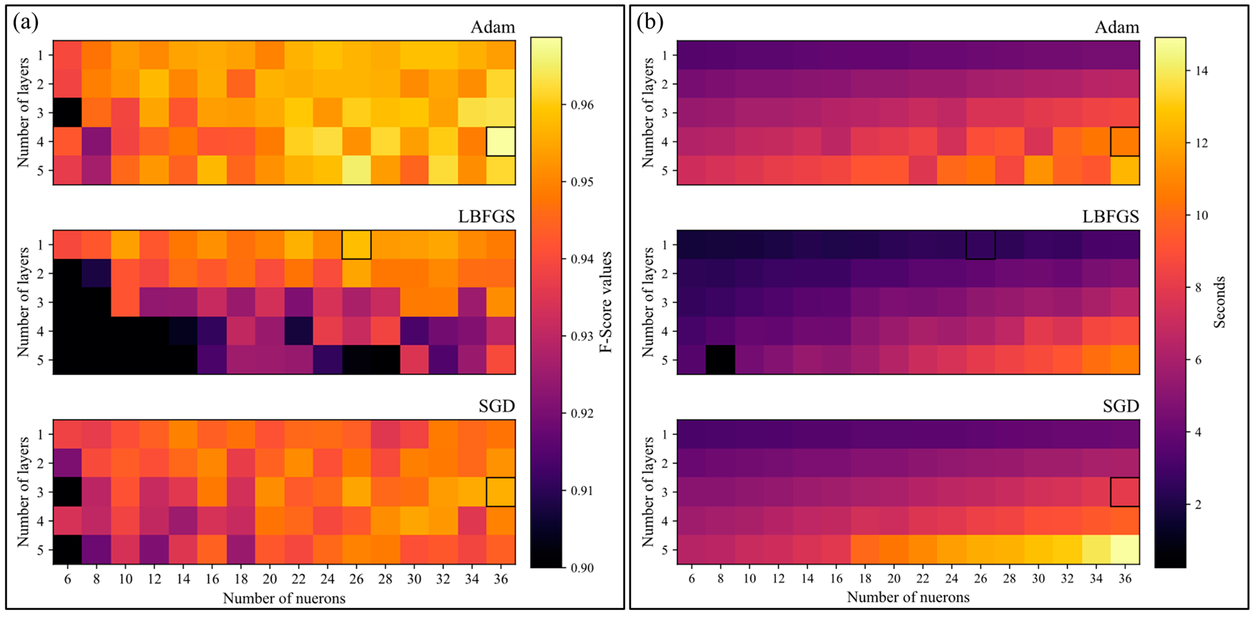
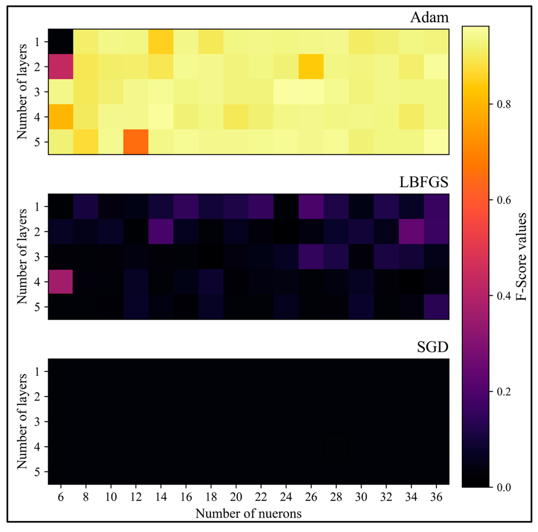
4.1. Number of Layers and Neurons

Figure 4 presents the F-score and computation time values of the ANN models with different topologies (i.e., number of layers and neurons) using three learning algorithms (i.e., Adam, LBFGS, and SGD). It should be noted that the Relu was considered in this step due to the extensive application of this activation function [90,91]. ANN topologies with one to five layer(s) with a step of one layer and a number of neurons from 6 to 36 with a step of 2 neurons were employed as small-to-medium-sized ANN models. The results also demonstrate the effect of different learning algorithms for mangrove ecosystem mapping using the ANN algorithm. Based on the results (see Figure 4a), the best ANN topologies for Adam, LBFGS, and SGD learning algorithms, respectively, were four layers with 36 neurons (F-score of 0.97) in each, one layer with 26 neurons (F-score of 0.95), and three layers with 36 neurons (F-score of 0.95) in each, respectively. Additionally, it was observed that the Adam learning algorithm had more consistent classification results (i.e., convergence with higher overall accuracies) with an average F-score value of 0.95 (±1%). The SGD had similar behavior with an average F-score value of 0.94 (±1.1%), while the LBFGS had a weaker performance with an average F-score value of 0.90 (±11%) and one divergence case (i.e., dissatisfaction of the loss function). Furthermore, over 20% of the ANN topologies with the LBFGS learning algorithm obtained lower F-score values than 0.90. Meanwhile, computation time generally had a consistent manner for all three learning algorithms. The computational time generally increased as the number of layers and neurons increased, with more dependency on the number of neurons (see Figure 4b). Regarding the computation time (i.e., training phase), the LBFGS entailed lower computation time with an average of 4.5 s, while the other two required approximately 6.5 s on average. It should be noted that the relative difference among computational times would increase when using more features or producing mangrove ecosystem maps of large-scale areas. Therefore, the time criterion could be considered an additional factor in identifying a suitable ANN topology.

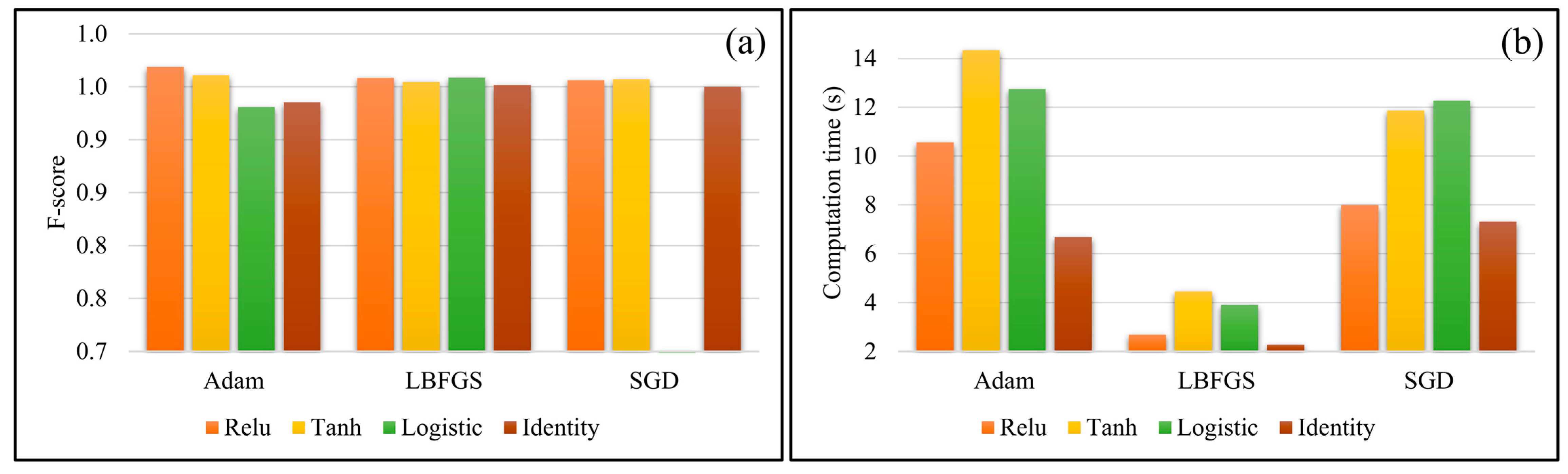
4.2. Activation Function
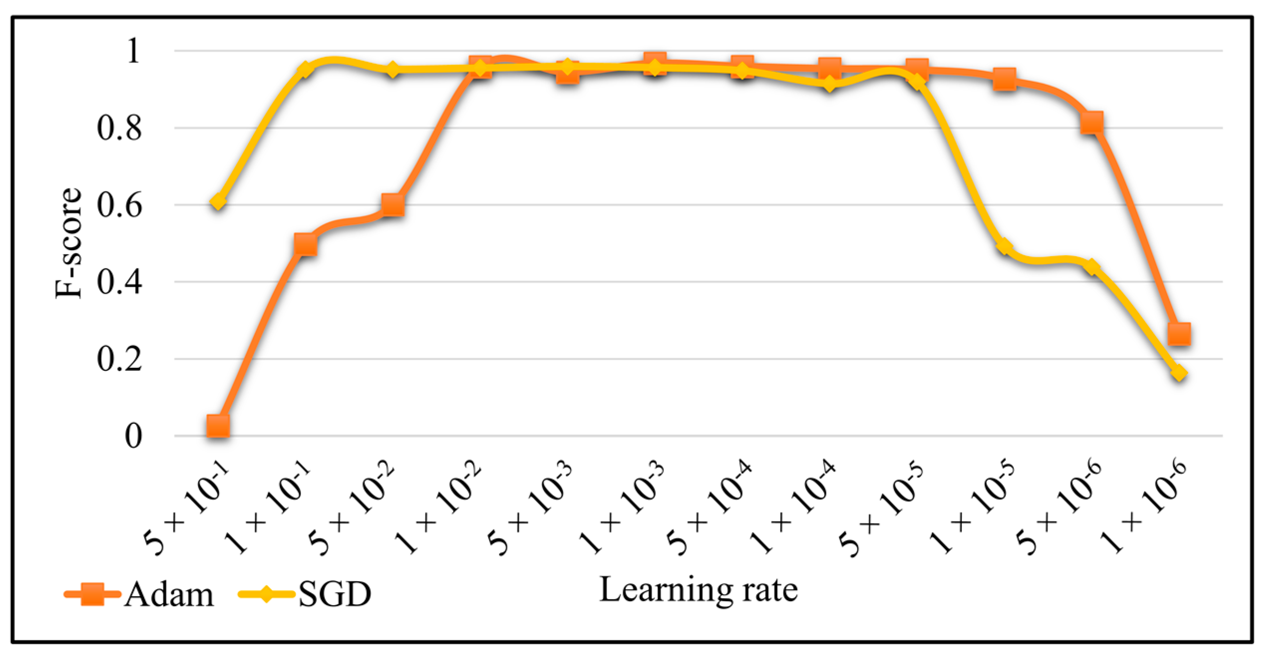
As stated in Section 4.1, the Relu was considered as the activation function to determine the best topologies for each learning algorithm. Adopting the best topologies from the previous section, the effect of four activation functions were explored. The results (see Figure 5) proved the capability of the Relu over other activation functions of Tanh, Logistic, and Identity. These results are in agreement with previous literature suggesting the high capability of the Relu activation function [90,91]. In particular, the Relu achieved higher F-score values, and in close competitions, required lower computation times. Furthermore, the results suggested a lower dependency of the ANN model on its activation function, especially based on the achieved accuracy (i.e., F-score value) when the best topology was identified. Moreover, the Identity entailed lower computation time, especially compared with Tanh and Logistic activation functions, and the combination of SGD and the Logistic led to inconsistent results with no convergence, making it less appropriate.

4.3. Learning Rate

After determining the three ANN models (i.e., for each learning algorithm), the effects of learning rates were explored. It is worth noting that only Adam and SGD support different learning rate values, so the investigations were relevant for these two learning algorithms. In this regard, 12 learning rate values ranging between 1 × 10⁶ and 0.5 were applied. The results (see Figure 6) presented similar behaviors for Adam and SGD when different learning rates were considered to train the ANN model. In particular, the ANN models with both learning algorithms achieved low F-score values when the learning rate values were very high or very low. In fact, very low learning rate values cause the ANNs not to converge in a limited number of iterations, while high values of learning rate make the algorithm jump from local minimums, not being able to converge into the best answer. This also indicated a high dependency of the ANN model on the learning rate value, which should be considered to ensure the most optimal classification result.

4.4. Mangrove Ecosystem Maps

After analyzing different ANN topologies and specifications in the previous sections, the best ANN models with three learning algorithms were applied to classify the mangrove ecosystem. Figure 7 shows the confusion matrices of the produced thematic maps, computed using independent test samples. The confusion matrices are generally diagonal in all cases (i.e., three learning algorithms), and few confusions happened. In particular, the highest confusions were between Shallow water and Tidal zone and between Urban and Barren. The former was mainly rooted in the fact that these classes have high similarity because of the water fluctuations (i.e., due to tides) and, thus, make it challenging to fully separate them. The latter was primarily associated with the materials used for residential roof construction over the study area, which was similar to Barren (bare soil). Furthermore, a minor confusion was observed between Mangrove and Vegetation and Mudflat. The first (i.e., Mangrove and Vegetation) was related to the slight similarity between these two vegetated classes. The second (i.e., Mangrove and Mudflat) mostly occurred due to the existence of mixed pixels as the result of their proximity at the boundary of each class. Table 2 also provides other statistical criteria derived from the confusion matrices. It can be seen that three ANN models obtained high PAs and UAs in each class. Overall, Mangrove and Mudflat classes had the first and second highest PAs and UAs on average. In contrast, Shallow water and Tidal zone obtained the lowest PAs and UAs on average using ANN models with three different learning algorithms. This could be associated with their similarity due to the water level changes.
The produced maps (i.e., only classes within the mangrove ecosystem) with a 10 m spatial resolution using different ANN models are presented in Figure 8. Based on the visual interpretation, the produced maps had acceptable accuracies, suggesting the high capability of combining the ANN algorithm and seasonal multi-source remote sensing data for mangrove ecosystem mapping. Overall, mangrove areas were delineated precisely, with higher accuracies through the Adam, LBFGS, and SDG algorithms, respectively. All three ANN models were also capable of correctly classifying most of the mangrove areas with small areas or narrow patches that extend along the coastal areas, where the highest capability was observed for the ANN model with the Adam learning algorithm. However, some mangrove regions were still not detected correctly due to the fact of being too sparse and fragmented. This would be effectively resolved using satellite images with higher spatial resolutions [46]. In particular, based on Figure 8, it can be seen that the Adam learning algorithm had the best performance in depicting mangrove areas and distinguishing Mangrove and Mudflat. In contrast, this happened with lower accuracy for other learning algorithms, especially SGD, which could not discriminate the small patches of Mudflat among Mangrove. Additionally, the middle parts of water bodies with higher depths were correctly identified by Adam and SGD, while there existed several misclassifications with the Tidal zone when using the LFBGS learning algorithm.
The agreements between produced mangrove maps were also computed to obtain a quantitative measure of the differences among these maps. It was observed that nearly 90% of pixels had identical labels, and other disagreements appeared primarily between the water classes (i.e., Deep water and Shallow water) and Tidal zone, while the minority was related to the Mangrove and Mudflat classes.

5. Discussion

In this section, first, a few general remarks are provided. Then, three different analyses are presented to provide a more comprehensive overview of the performance of the ANN models. Although the input data in these analyses were related to the mangrove ecosystem, the reached implications primarily manifest the behavior of ANN models that could elucidate a path for readers implementing ANN algorithms over different study areas.

5.1. General Remarks

Mangrove ecosystems provide many economic, ecological, and environmental benefits for humans and their surroundings [92]. Some of these services are unique, which rationalizes the importance of conserving mangrove ecosystems from degradation. One of the efficient approaches for mangrove mapping is to employ remote sensing data to frequently monitor these natural resources and take the necessary actions to avoid their further loss [93]. In this regard, the machine learning algorithms, such as ANN, that were investigated in this paper can be incorporated to obtain highly accurate information about the mangrove ecosystems. Currently, satellite images with medium spatial resolutions, such as Sentinel-1, Sentinel-2, and Landsat archives, can be accessed with no cost, permitting monitoring of these ecosystems with optimized costs in spatial and temporal directions [22]. Indeed, these satellites could be effectively employed by different national and local organizations regarding the preservation practices of mangrove ecosystems from decay. However, it should be considered that more accurate information, especially on sparse mangroves and narrow mangrove patches, requires the utility of satellite images with higher spatial resolutions, and the high cost of these images is the primary obligation [94].
The ANN models proved to be capable of producing accurate mangrove ecosystem maps. Likewise, the results and further discussions could elucidate the path for other researchers to implement the ANN algorithm in other areas. Additionally, the proven potential of the ANN algorithm in this study may encourage other researchers to suppose achieving satisfactory results in other mangrove ecosystems even with more complex conditions. For instance, it is expected to obtain accurate results using the ANN algorithm in other mangrove ecosystems with other classes such as terrestrial forest, other wetland types, shrubs, and other vegetated communities. This is because other vegetated communities and wetlands have a higher rate of spectral similarity with mangroves [95]. This would affect the classification procedure by decreasing the separability of classes and, thus, robust algorithms are vital for accurate mapping. Furthermore, Three ANN models performed satisfactorily, and the achieved PAs and UAs (see Table 2) suggested that the ensemble of ANN models can enhance the results, which could be investigated in future studies. This is mainly due to the fact that each ANN model obtained higher accuracies in different classes over the study area.
In this study, the satellite images were collected from GEE. This cloud-based platform uses high-performance parallel computing that allows for the application of preprocessing steps on numerous images [20,68]. Consequently, it can help to reduce the required time for applying preprocessing steps that are almost repetitive procedures and can lead to a decrease in the dedicated time [46,96]. Despite these massive advantages, this cloud platform does not currently support ANN models in its base form (i.e., JavaScript API); hence, the experiments should be taken in another platform. Here, the Google Colab platform and the scikit-learn package were used in support of the implemented methodology so that it can be applied at a low cost by any users around the world.
The results of this study confirmed the capability of the implemented ANN model for mangrove ecosystem mapping. Accordingly, this algorithm could be implemented to produce an accurate baseline of mangrove ecosystems in any region. Additionally, the utility of charge-free satellite images (i.e., Sentinel-1 and Sentinel-2) and cloud computing platforms allow for frequent mangrove mapping at a low cost. In this regard, the temporal evolutions and changes in mangrove ecosystems can be mapped in previous years based on the availability of Sentinel-1 and Sentinel-2 images and the following years. This framework permits consistent monitoring of mangrove ecosystems and creates the opportunity to enact practical workflows to preserve these natural resources, especially in protected areas, from adverse anthropogenic and natural processes. Furthermore, frequent monitoring through such a reproducible approach can assist in assessing the applied practices, such as conservation planning and mangrove plantation, to support sustainable development.

5.2. Impact of Data Standardization

Input data transformation has been recognized as an impactful preprocessing task when using machine learning algorithms such as ANN models [97]. Accordingly, the remote sensing data of this study were transformed using the standard scaler approach (i.e., removing the mean and scaling to unit variance). However, an analysis was also performed to investigate the impact of data transformation/standardization on ANN models based on three different learning algorithms. ANN models with different topologies were retrained using raw input features. Based on Figure 9, all ANN models failed to retain their behavior in comparison to using transformed input data (see Figure 4). In particular, the ANN models with the LBFGS and SGD learning algorithms failed to converge in almost all cases. However, the ANN model in which the Adam learning algorithm was employed performed more consistently. In fact, this analysis demonstrated the capability of the Adam learning algorithm to handle untransformed input data.

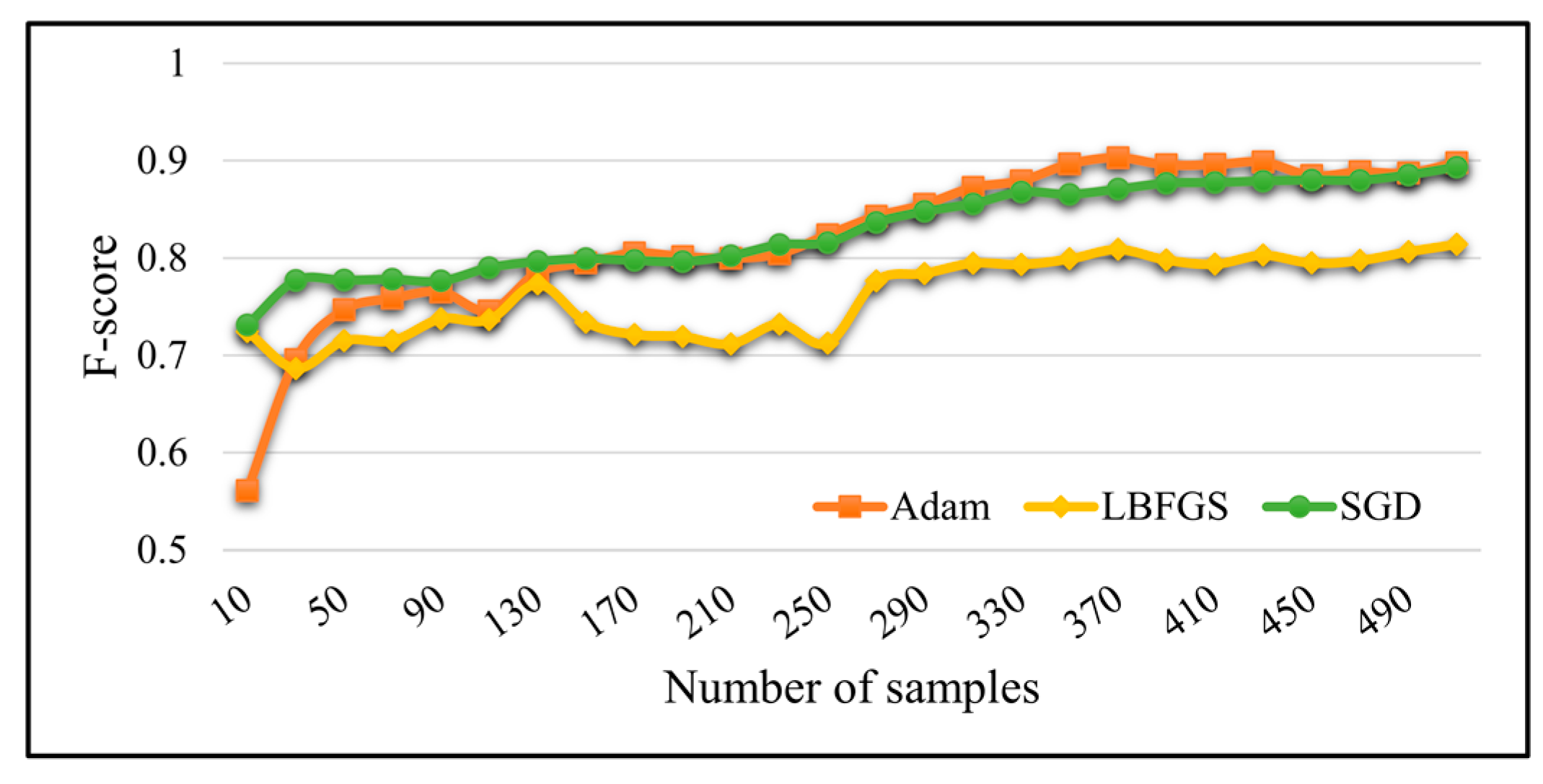
5.3. Impact of Limited Training Samples

It is already known that training samples are required to support the training phase of any supervised machine learning algorithm. Furthermore, it is accredited that collecting training samples, either through in situ field campaigns or visual interpretation of high-resolution images, is time consuming and resource intensive [98]. Therefore, it is more convenient to develop efficient approaches or incorporate robust machine learning algorithms that require a limited number of training samples [99,100]. Accordingly, the impact of limited training samples on the performance of the ANN models was also explored. To this end, only a limited number of training samples from the original set (see Section 3.1) was considered in this section. In particular, the number of training samples for each class was set between 10 and 500 to evaluate the performance of ANN models. Figure 10 illustrates the outcome of using a limited number of training samples for mangrove ecosystem mapping. It is evident that three ANN models experienced an F-score fall compared with the case of using whole training samples. For example, the F-score values of the ANN models with the Adam, LBFGS, and SGD learning algorithms, respectively, decreased by 7%, 16%, and 7%, considering their best case using a limited number of training samples. Furthermore, Figure 10 shows that the LBFGS relatively tends to obtain lower accuracies when the number of training samples was limited.

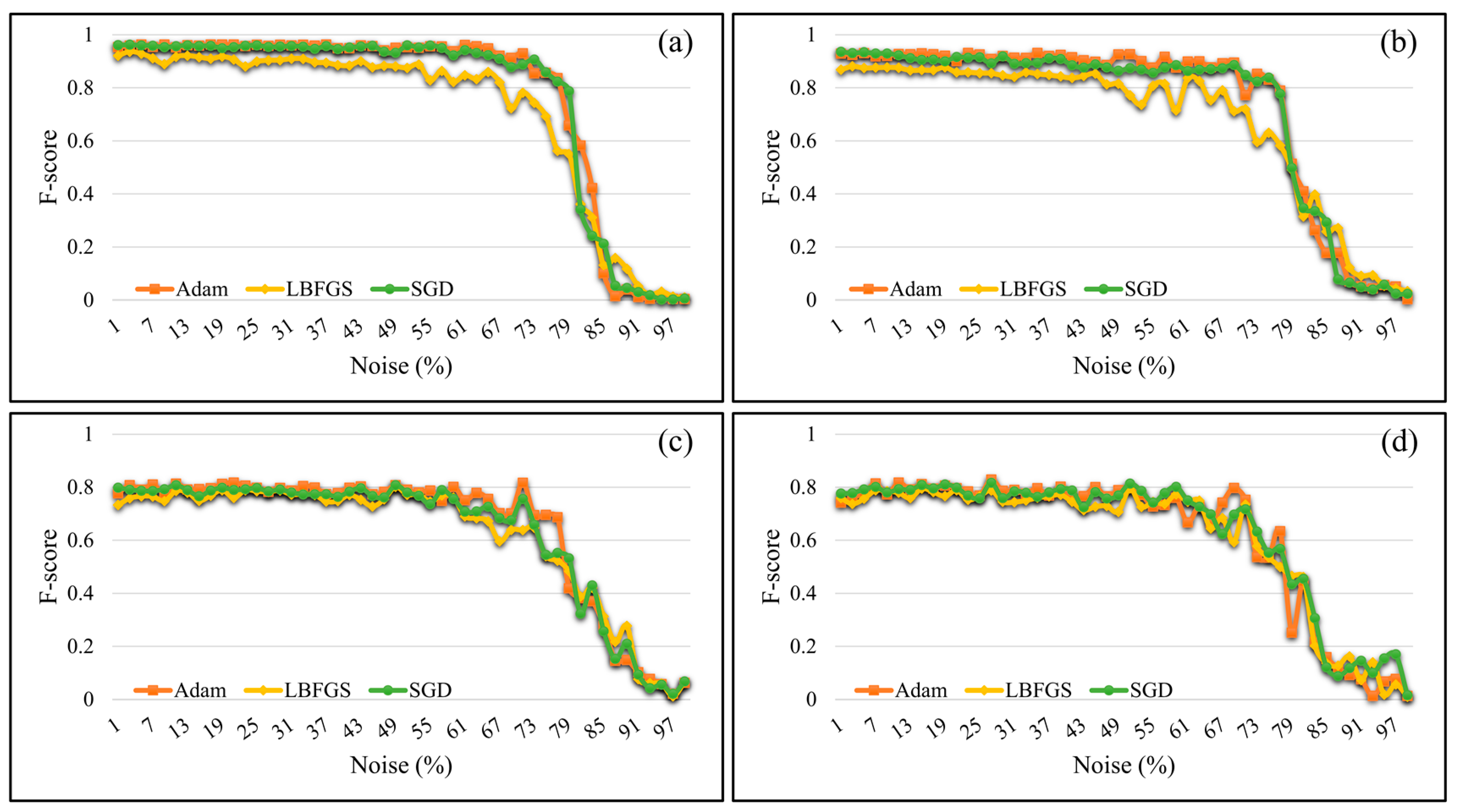
5.4. Impact of Noise Labels

The quality of training samples can directly influence the classification results. As such, the existence of noise labels (i.e., training samples with wrong labels), from any source, in the training samples can adversely affect the performance of machine learning algorithms [101]. For instance, mislabeling of 25% of the training samples reduced the OA of the RF up to 10%. Additionally, based on experimental results, the KC obtained using the KNN classifier decreased by approximately 35% when 28% of the training samples had wrong labels [101]. In this perspective, the performance of the best ANN models was examined in the case of the presence of noise labels. To this end, the labels of a portion (in percentage) of the training samples were randomly changed to other classes. It should be noted that an equal percentage was applied to training samples of each class. Additionally, the impact of noise labels was investigated based on a different number of training samples to identify whether there was any relationship between these two factors. It was observed (see Figure 11) that ANN models were minorly affected by noise labels when the noise label percentage was set between 1% and 100%, and a more dramatic decrease in the F-score occurred when over 60% of training samples were subjected to label change. Furthermore, no direct relationship was found between the number of training samples and noise labels.

5.5. Contribution of Multi-Temporal and Multi-Source Images

Using multi-temporal and multi-source remote sensing imagery is recognized as a practical approach to obtaining higher land cover (e.g., wetlands) classification results [102]. This is rooted in the fact that different remote sensing data sources could provide complementary information of the Earth’s surface. For instance, multi-spectral and SAR data sets provide spectral and physical properties of the Earth’s surface, respectively. Furthermore, multi-temporal remote sensing could provide discriminative information about different classes with dynamic characteristics, reducing the confusion of existing classes and improving the classification results [21,103].
Regarding the contribution of the multi-source remote sensing data, the best ANN models were incorporated to map the mangrove ecosystem using single-source data sets. It was observed that the obtained F-score value using multi-spectral (i.e., Sentinel-2) images for the best ANN model was 0.95, which was nearly 2% lower than using multi-source data sets. Furthermore, the results revealed that incorporating only the SAR data set could not achieve satisfactory results (i.e., F-score = 0.75). The results indicated that the utility of multi-source remote sensing could enhance the classification results and could lead to accurate mangrove maps. This improvement would be more considerable in locations with more complex conditions [65].
Moreover, the best ANN model was employed to examine the effects of using multi-temporal data sets in the classification results. In this regard, single-season data sets were fed into the best ANN model, and it was observed that no single-season data set achieved higher classification accuracy. In particular, the spring, summer, autumn, and winter data sets achieved F-score values of 0.94, 0.91, 0.92, and 0.92, respectively. These values were 3%, 6%, 5%, and 5% lower than the accuracy of the map using multi-temporal data sets.

6. Conclusions

This paper investigated the applicability of integrating ANN models with multi-temporal and multi-source remote sensing data. The results indicated the high potential of the ANN models, especially the ANN model with the Adam learning algorithm for mangrove ecosystem mapping (F-score = 0.97). Furthermore, the results demonstrated the higher consistency of ANN models when incorporating the Adam learning algorithm. It was also observed that all three ANN models achieved high UAs and PAs, although higher class accuracies were reached by different models. This showed the potential improvement in classification accuracy by using an ensemble approach to integrate the classification results of ANN models with different learning algorithms. Additionally, it was concluded that data standardization is an unavoidable preprocessing step when using the SGD and LFBGS learning algorithms. The ANN models proved to have a high resistance in noise label conditions (i.e., training samples with wrong labels), and the classification results with a limited number of samples were subjected to accuracy loss with more effects when using the LBFGS learning algorithm. Finally, it was observed that incorporating multi-temporal and multi-source remote sensing data sets could enhance the mangrove classification results, and it is expected to see more improvement in other complex ecosystems.

Author Contributions

Conceptualization, A.G., S.A.A. and M.A.; methodology, A.G. and S.A.A.; software, A.G. and S.A.A.; validation, A.G. and S.A.A.; formal analysis, A.G. and S.A.A.; investigation, A.G. and S.A.A.; resources, A.G. and S.A.A.; data curation, A.G.; writing—original draft preparation, A.G. and S.A.A.; writing—review and editing, A.G., S.A.A., M.A., A.M. and S.J.; visualization, A.G. and S.A.A.; supervision, M.A., A.M. and S.J.; project administration, A.G. All authors have read and agreed to the published version of the manuscript.

Funding

This research received no external funding.

Data Availability Statement

The Sentinel-1 (Sentinel-1 SAR GRD in Earth Engine Data Catalog. Available online: https://developers.google.com/earth-engine/datasets/catalog/COPERNICUS_S1_GRD (accessed on 19 November 2021)) and Sentinel-2 (Sentinel-2 MSI in Earth Engine Data Catalog. Available online: https://developers.google.com/earth-engine/datasets/catalog/COPERNICUS_S2 (accessed on 19 November 2021)) satellite images were collected from the Google Earth Engine cloud computing platform and are freely available for all interested users.

Acknowledgments

The authors would like to thank the European Space Agency (ESA) for freely providing Sentinel-1 and Sentinel-2 satellite data.

Conflicts of Interest

The authors declare no conflict of interest.

References

  1. Lee, W.K.; Tay, S.H.X.; Ooi, S.K.; Friess, D.A. Potential short wave attenuation function of disturbed mangroves. Estuar. Coast. Shelf Sci. 2021, 248, 106747. [Google Scholar] [CrossRef]
  2. Maria, M.; Losada, I.J. Predicting the evolution of coastal protection service with mangrove forest age. Coast. Eng. 2021, 168, 103922. [Google Scholar]
  3. Kandasamy, K.; Rajendran, N.; Balakrishnan, B.; Thiruganasambandam, R.; Narayanasamy, R. Carbon sequestration and storage in planted mangrove stands of Avicennia marina. Reg. Stud. Mar. Sci. 2021, 43, 101701. [Google Scholar] [CrossRef]
  4. Rovai, A.S.; Coelho-Jr, C.; de Almeida, R.; Cunha-Lignon, M.; Menghini, R.P.; Twilley, R.R.; Cintrón-Molero, G.; Schaeffer-Novelli, Y. Ecosystem-level carbon stocks and sequestration rates in mangroves in the Cananéia-Iguape lagoon estuarine system, southeastern Brazil. For. Ecol. Manag. 2021, 479, 118553. [Google Scholar] [CrossRef]
  5. Sundaramanickam, A.; Nithin, A.; Balasubramanian, T. Role of Mangroves in Pollution Abatement. In Mangroves: Ecology, Biodiversity and Management; Springer: Berlin, Germany, 2021; pp. 257–278. [Google Scholar]
  6. Mafi Gholami, D.; Baharlouii, M. Monitoring long-term mangrove shoreline changes along the northern coasts of the Persian Gulf and the Oman Sea. Emerg. Sci. J. 2019, 3, 88–100. [Google Scholar] [CrossRef] [Green Version]
  7. Thatoi, H.; Samantaray, D.; Das, S.K. The genus Avicennia, a pioneer group of dominant mangrove plant species with potential medicinal values: A review. Front. Life Sci. 2016, 9, 267–291. [Google Scholar] [CrossRef] [Green Version]
  8. Baishya, S.; Banik, S.K.; Choudhury, M.D.; Talukdar, D.D.; Talukdar, A.D. Therapeutic Potentials of Littoral Vegetation: An Antifungal Perspective. In Biotechnological Utilization of Mangrove Resources; Elsevier: Amsterdam, The Netherlands, 2020; pp. 275–292. [Google Scholar]
  9. Rahman, K.-S.; Islam, M.N.; Ahmed, M.U.; Bosma, R.H.; Debrot, A.O.; Ahsan, M.N. Selection of mangrove species for shrimp based silvo-aquaculture in the coastal areas of Bangladesh. J. Coast. Conserv. 2020, 24, 59. [Google Scholar] [CrossRef]
  10. Seary, R.; Spencer, T.; Bithell, M.; McOwen, C. Measuring mangrove-fishery benefits in the Peam Krasaop Fishing Community, Cambodia. Estuar. Coast. Shelf Sci. 2021, 248, 106918. [Google Scholar] [CrossRef]
  11. Eddy, S.; Milantara, N.; Sasmito, S.D.; Kajita, T.; Basyuni, M. Anthropogenic drivers of mangrove loss and associated carbon emissions in South Sumatra, Indonesia. Forests 2021, 12, 187. [Google Scholar] [CrossRef]
  12. Goldberg, L.; Lagomasino, D.; Thomas, N.; Fatoyinbo, T. Global declines in human-driven mangrove loss. Glob. Chang. Biol. 2020, 26, 5844–5855. [Google Scholar] [CrossRef]
  13. Sippo, J.Z.; Lovelock, C.E.; Santos, I.R.; Sanders, C.J.; Maher, D.T. Mangrove mortality in a changing climate: An overview. Estuar. Coast. Shelf Sci. 2018, 215, 241–249. [Google Scholar] [CrossRef]
  14. Polidoro, B.A.; Carpenter, K.E.; Collins, L.; Duke, N.C.; Ellison, A.M.; Ellison, J.C.; Farnsworth, E.J.; Fernando, E.S.; Kathiresan, K.; Koedam, N.E.; et al. The loss of species: Mangrove extinction risk and geographic areas of global concern. PLoS ONE 2010, 5, e10095. [Google Scholar] [CrossRef]
  15. Sathish, C.; Dayaram, N.A.; Bharti, V.S.; Jaiswar, A.K.; Deshmukhe, G. Estimation of extent of the mangrove defoliation caused by insect Hyblaea puera (Cramer, 1777) around Dharamtar creek, India using Sentinel 2 images. Reg. Stud. Mar. Sci. 2021, 48, 102054. [Google Scholar] [CrossRef]
  16. Belenok, V.; Noszczyk, T.; Hebryn-Baidy, L.; Kryachok, S. Investigating anthropogenically transformed landscapes with remote sensing. Remote Sens. Appl. Soc. Environ. 2021, 24, 100635. [Google Scholar] [CrossRef]
  17. Maurya, K.; Mahajan, S.; Chaube, N. Remote sensing techniques: Mapping and monitoring of mangrove ecosystem—A review. Complex Intell. Syst. 2021, 7, 2797–2818. [Google Scholar] [CrossRef]
  18. Pham, T.D.; Xia, J.; Ha, N.T.; Bui, D.T.; Le, N.N.; Tekeuchi, W. A review of remote sensing approaches for monitoring blue carbon ecosystems: Mangroves, seagrassesand salt marshes during 2010–2018. Sensors 2019, 19, 1933. [Google Scholar] [CrossRef] [PubMed] [Green Version]
  19. Thakur, S.; Mondal, I.; Ghosh, P.B.; Das, P.; De, T.K. A review of the application of multispectral remote sensing in the study of mangrove ecosystems with special emphasis on image processing techniques. Spat. Inf. Res. 2020, 28, 39–51. [Google Scholar] [CrossRef]
  20. Amani, M.; Mahdavi, S.; Kakooei, M.; Ghorbanian, A.; Brisco, B.; Delancey, E.; Toure, S.; Reyes, E.L. Wetland Change Analysis in Alberta, Canada using Four Decades of Landsat Imagery. IEEE J. Sel. Top. Appl. Earth Obs. Remote Sens. 2021, 14, 10314–10335. [Google Scholar] [CrossRef]
  21. Zhao, C.; Qin, C.-Z. 10-m-resolution mangrove maps of China derived from multi-source and multi-temporal satellite observations. ISPRS J. Photogramm. Remote Sens. 2020, 169, 389–405. [Google Scholar] [CrossRef]
  22. Wang, L.; Jia, M.; Yin, D.; Tian, J. A review of remote sensing for mangrove forests: 1956–2018. Remote Sens. Environ. 2019, 231, 111223. [Google Scholar] [CrossRef]
  23. Hati, J.P.; Samanta, S.; Chaube, N.R.; Misra, A.; Giri, S.; Pramanick, N.; Gupta, K.; Majumdar, S.D.; Chanda, A.; Mukhopadhyay, A.; et al. Mangrove classification using airborne hyperspectral AVIRIS-NG and comparing with other spaceborne hyperspectral and multispectral data. Egypt. J. Remote Sens. Space Sci. 2021, 24, 273–281. [Google Scholar]
  24. Purwanto, A.D.; Asriningrum, W. Identification of mangrove forests using multispectral satellite imageries. Int. J. Remote Sens. Earth Sci. 2019, 16, 63–86. [Google Scholar] [CrossRef]
  25. Li, Q.; Wong, F.K.K.; Fung, T. Mapping multi-layered mangroves from multispectral, hyperspectral, and LiDAR data. Remote Sens. Environ. 2021, 258, 112403. [Google Scholar] [CrossRef]
  26. Abdel-Hamid, A.; Dubovyk, O.; El-Magd, A.; Menz, G. Mapping mangroves extents on the Red Sea coastline in Egypt using polarimetric SAR and high resolution optical remote sensing data. Sustainability 2018, 10, 646. [Google Scholar] [CrossRef] [Green Version]
  27. Chen, N. Mapping mangrove in Dongzhaigang, China using Sentinel-2 imagery. J. Appl. Remote Sens. 2020, 14, 14508. [Google Scholar] [CrossRef]
  28. Osei Darko, P.; Kalacska, M.; Arroyo-Mora, J.P.; Fagan, M.E. Spectral Complexity of Hyperspectral Images: A New Approach for Mangrove Classification. Remote Sens. 2021, 13, 2604. [Google Scholar] [CrossRef]
  29. Ashiagbor, G.; Asante, W.A.; Quaye-Ballard, J.A.; Forkuo, E.K.; Acheampong, E.; Foli, E. Mangrove mapping using Sentinel-1 data for improved decision support on sustainable conservation and restoration interventions in the Keta Lagoon Complex Ramsar Site, Ghana. Mar. Freshw. Res. 2021, 72, 1588–1601. [Google Scholar] [CrossRef]
  30. Bindu, G.; Rajan, P.; Jishnu, E.S.; Joseph, K.A. Carbon stock assessment of mangroves using remote sensing and geographic information system. Egypt. J. Remote Sens. Sp. Sci. 2020, 23, 1–9. [Google Scholar] [CrossRef]
  31. Komiyama, A.; Poungparn, S.; Kato, S. Common allometric equations for estimating the tree weight of mangroves. J. Trop. Ecol. 2005, 21, 471–477. [Google Scholar] [CrossRef]
  32. Hu, T.; Zhang, Y.; Su, Y.; Zheng, Y.; Lin, G.; Guo, Q. Mapping the global mangrove forest aboveground biomass using multisource remote sensing data. Remote Sens. 2020, 12, 1690. [Google Scholar] [CrossRef]
  33. Lucas, R.; Van De Kerchove, R.; Otero, V.; Lagomasino, D.; Fatoyinbo, L.; Omar, H.; Satyanarayana, B.; Dahdouh-Guebas, F. Structural characterisation of mangrove forests achieved through combining multiple sources of remote sensing data. Remote Sens. Environ. 2020, 237, 111543. [Google Scholar] [CrossRef]
  34. Halder, S.; Samanta, K.; Das, S.; Pathak, D. Monitoring the inter-decade spatial--temporal dynamics of the Sundarban mangrove forest of India from 1990 to 2019. Reg. Stud. Mar. Sci. 2021, 44, 101718. [Google Scholar] [CrossRef]
  35. Parida, B.R.; Kumar, P. Mapping and dynamic analysis of mangrove forest during 2009–2019 using landsat-5 and sentinel-2 satellite data along Odisha Coast. Trop. Ecol. 2020, 61, 538–549. [Google Scholar] [CrossRef]
  36. Elmahdy, S.I.; Ali, T.A.; Mohamed, M.M.; Howari, F.M.; Abouleish, M.; Simonet, D. Spatiotemporal Mapping and Monitoring of Mangrove Forests Changes From 1990 to 2019 in the Northern Emirates, UAE Using Random Forest, Kernel Logistic Regression and Naive Bayes Tree Models. Front. Environ. Sci. 2020, 8, 102. [Google Scholar] [CrossRef]
  37. Behera, M.D.; Barnwal, S.; Paramanik, S.; Das, P.; Bhattyacharya, B.K.; Jagadish, B.; Roy, P.S.; Ghosh, S.M.; Behera, S.K. Species-Level Classification and Mapping of a Mangrove Forest Using Random Forest—Utilisation of AVIRIS-NG and Sentinel Data. Remote Sens. 2021, 13, 2027. [Google Scholar] [CrossRef]
  38. Kamal, M.; Phinn, S.; Johansen, K. Object-based approach for multi-scale mangrove composition mapping using multi-resolution image datasets. Remote Sens. 2015, 7, 4753–4783. [Google Scholar] [CrossRef] [Green Version]
  39. Mondal, P.; Liu, X.; Fatoyinbo, T.E.; Lagomasino, D. Evaluating combinations of sentinel-2 data and machine-learning algorithms for mangrove mapping in West Africa. Remote Sens. 2019, 11, 2928. [Google Scholar] [CrossRef] [Green Version]
  40. Maung, W.S.; Sasaki, J. Assessing the Natural Recovery of Mangroves after Human Disturbance Using Neural Network Classification and Sentinel-2 Imagery in Wunbaik Mangrove Forest, Myanmar. Remote Sens. 2021, 13, 52. [Google Scholar] [CrossRef]
  41. Zhang, X.; Treitz, P.M.; Chen, D.; Quan, C.; Shi, L.; Li, X. Mapping mangrove forests using multi-tidal remotely-sensed data and a decision-tree-based procedure. Int. J. Appl. Earth Obs. Geoinf. 2017, 62, 201–214. [Google Scholar] [CrossRef]
  42. Toosi, N.B.; Soffianian, A.R.; Fakheran, S.; Pourmanafi, S.; Ginzler, C.; Waser, L.T. Comparing different classification algorithms for monitoring mangrove cover changes in southern Iran. Glob. Ecol. Conserv. 2019, 19, e00662. [Google Scholar] [CrossRef]
  43. Held, A.; Ticehurst, C.; Lymburner, L.; Williams, N. High resolution mapping of tropical mangrove ecosystems using hyperspectral and radar remote sensing. Int. J. Remote Sens. 2003, 24, 2739–2759. [Google Scholar] [CrossRef]
  44. Xia, J.; Yokoya, N.; Pham, T.D. Probabilistic mangrove species mapping with multiple-source remote-sensing datasets using label distribution learning in Xuan Thuy National Park, Vietnam. Remote Sens. 2020, 12, 3834. [Google Scholar] [CrossRef]
  45. Zhang, H.; Wang, T.; Liu, M.; Jia, M.; Lin, H.; Chu, L.M.; Devlin, A.T. Potential of combining optical and dual polarimetric SAR data for improving mangrove species discrimination using rotation forest. Remote Sens. 2018, 10, 467. [Google Scholar] [CrossRef] [Green Version]
  46. Ghorbanian, A.; Zaghian, S.; Asiyabi, R.M.; Amani, M.; Mohammadzadeh, A.; Jamali, S. Mangrove Ecosystem Mapping Using Sentinel-1 and Sentinel-2 Satellite Images and Random Forest Algorithm in Google Earth Engine. Remote Sens. 2021, 13, 2565. [Google Scholar] [CrossRef]
  47. Guo, M.; Yu, Z.; Xu, Y.; Huang, Y.; Li, C. ME-Net: A Deep Convolutional Neural Network for Extracting Mangrove Using Sentinel-2A Data. Remote Sens. 2021, 13, 1292. [Google Scholar] [CrossRef]
  48. Wan, L.; Zhang, H.; Lin, G.; Lin, H. A small-patched convolutional neural network for mangrove mapping at species level using high-resolution remote-sensing image. Ann. GIS 2019, 25, 45–55. [Google Scholar] [CrossRef]
  49. Wang, L.; Silván-Cárdenas, J.L.; Sousa, W.P. Neural network classification of mangrove species from multi-seasonal Ikonos imagery. Photogramm. Eng. Remote Sens. 2008, 74, 921–927. [Google Scholar] [CrossRef] [Green Version]
  50. Alireza, S.M.; Mansour, J.B. Satellite based assessment of the area and changes in the Mangrove ecosystem of the QESHM Island, Iran. J. Environ. Res. Dev. 2012, 7, 1052–1060. [Google Scholar]
  51. Sharifi, N.; Danehkar, A.; Robati, M.; Khorasani, N.A.; Rajaee, T. Developing decision algorithm for determination of protection zones in protected areas (case study: Hara Protected Area). Int. J. Environ. Sci. Technol. 2021, 18, 2237–2250. [Google Scholar] [CrossRef]
  52. Ghasemi, S.; Moghaddam, S.S.; Rahimi, A.; Damalas, C.A.; Naji, A. Phytomanagement of trace metals in mangrove sediments of Hormozgan, Iran, using gray mangrove (Avicennia marina). Environ. Sci. Pollut. Res. 2018, 25, 28195–28205. [Google Scholar] [CrossRef]
  53. Vahidi, F.; Fatemi, S.M.R.; Danehkar, A.; Moradi, A.M.; Nadushan, R.M. Patterns of mollusks (Bivalvia and Gastropoda) distribution in three different zones of Harra Biosphere Reserve, the Persian Gulf, Iran. Iran. J. Fish. Sci. 2021, 20, 1336–1353. [Google Scholar]
  54. Hajializadeh, P.; Safaie, M.; Naderloo, R.; Shojaei, M.G.; Gammal, J.; Villnäs, A.; Norkko, A. Species composition and functional traits of macrofauna in different mangrove habitats in the Persian gulf. Front. Mar. Sci. 2020, 7, 809. [Google Scholar] [CrossRef]
  55. Dadashi, M.; Ghaffari, S.; Bakhtiari, A.R.; Tauler, R. Multivariate curve resolution of organic pollution patterns in mangrove forest sediment from Qeshm Island and Khamir Port—Persian Gulf, Iran. Environ. Sci. Pollut. Res. 2018, 25, 723–735. [Google Scholar] [CrossRef] [PubMed]
  56. Zarezadeh, R.; Rezaee, P.; Lak, R.; Masoodi, M.; Ghorbani, M. Distribution and accumulation of heavy metals in sediments of the northern part of mangrove in Hara Biosphere Reserve, Qeshm Island (Persian Gulf). Soil Water Res. 2017, 12, 86–95. [Google Scholar] [CrossRef] [Green Version]
  57. Kazemi, A.; Bakhtiari, A.R.; Kheirabadi, N.; Barani, H.; Haidari, B. Distribution patterns of metals contamination in sediments based on type regional development on the intertidal coastal zones of the Persian Gulf, Iran. Bull. Environ. Contam. Toxicol. 2012, 88, 100–103. [Google Scholar] [CrossRef]
  58. Bunting, P.; Rosenqvist, A.; Lucas, R.M.; Rebelo, L.-M.; Hilarides, L.; Thomas, N.; Hardy, A.; Itoh, T.; Shimada, M.; Finlayson, C.M. The global mangrove watch—A new 2010 global baseline of mangrove extent. Remote Sens. 2018, 10, 1669. [Google Scholar] [CrossRef] [Green Version]
  59. Murray, N.J.; Phinn, S.R.; DeWitt, M.; Ferrari, R.; Johnston, R.; Lyons, M.B.; Clinton, N.; Thau, D.; Fuller, R.A. The global distribution and trajectory of tidal flats. Nature 2019, 565, 222–225. [Google Scholar] [CrossRef] [PubMed]
  60. Lohr, S.L. Sampling: Design and Analysis; CRC Press: Bocaton, FL, USA, 2019. [Google Scholar]
  61. Geiß, C.; Pelizari, P.A.; Schrade, H.; Brenning, A.; Taubenböck, H. On the effect of spatially non-disjoint training and test samples on estimated model generalization capabilities in supervised classification with spatial features. IEEE Geosci. Remote Sens. Lett. 2017, 14, 2008–2012. [Google Scholar]
  62. Sentinel Overview. Available online: https://sentinels.copernicus.eu/web/sentinel/missions (accessed on 31 October 2021).
  63. Gorelick, N.; Hancher, M.; Dixon, M.; Ilyushchenko, S.; Thau, D.; Moore, R. Google Earth Engine: Planetary-scale geospatial analysis for everyone. Remote Sens. Environ. 2017, 202, 18–27. [Google Scholar] [CrossRef]
  64. Amani, M.; Ghorbanian, A.; Ahmadi, S.A.; Kakooei, M.; Moghimi, A.; Mirmazloumi, S.M.; Moghaddam, S.H.A.; Mahdavi, S.; Ghahremanloo, M.; Parsian, S.; et al. Google Earth Engine Cloud Computing Platform for Remote Sensing Big Data Applications: A Comprehensive Review. IEEE J. Sel. Top. Appl. Earth Obs. Remote Sens. 2020, 13, 5326–5350. [Google Scholar] [CrossRef]
  65. Mahdavi, S.; Salehi, B.; Amani, M.; Granger, J.; Brisco, B.; Huang, W. A dynamic classification scheme for mapping spectrally similar classes: Application to wetland classification. Int. J. Appl. Earth Obs. Geoinf. 2019, 83, 101914. [Google Scholar] [CrossRef]
  66. Fekri, E.; Latifi, H.; Amani, M.; Zobeidinezhad, A. A Training Sample Migration Method for Wetland Mapping and Monitoring Using Sentinel Data in Google Earth Engine. Remote Sens. 2021, 13, 4169. [Google Scholar] [CrossRef]
  67. He, Y.; Dong, J.; Liao, X.; Sun, L.; Wang, Z.; You, N.; Li, Z.; Fu, P. Examining rice distribution and cropping intensity in a mixed single-and double-cropping region in South China using all available Sentinel 1/2 images. Int. J. Appl. Earth Obs. Geoinf. 2021, 101, 102351. [Google Scholar] [CrossRef]
  68. Ghorbanian, A.; Kakooei, M.; Amani, M.; Mahdavi, S.; Mohammadzadeh, A.; Hasanlou, M. Improved land cover map of Iran using Sentinel imagery within Google Earth Engine and a novel automatic workflow for land cover classification using migrated training samples. ISPRS J. Photogramm. Remote Sens. 2020, 167, 276–288. [Google Scholar] [CrossRef]
  69. Torres, R.; Snoeij, P.; Geudtner, D.; Bibby, D.; Davidson, M.; Attema, E.; Potin, P.; Rommen, B.; Floury, N.; Brown, M.; et al. GMES Sentinel-1 mission. Remote Sens. Environ. 2012, 120, 9–24. [Google Scholar] [CrossRef]
  70. Liu, X.; Fatoyinbo, T.E.; Thomas, N.M.; Guan, W.W.; Zhan, Y.; Mondal, P.; Lagomasino, D.; Simard, M.; Trettin, C.C.; Deo, R.; et al. Large-scale High-resolution Coastal Mangrove Forests Mapping across West Africa with Machine Learning Ensemble and Satellite Big Data. Front. Earth Sci. 2021, 8, 677. [Google Scholar] [CrossRef]
  71. Mullissa, A.; Vollrath, A.; Odongo-Braun, C.; Slagter, B.; Balling, J.; Gou, Y.; Gorelick, N.; Reiche, J. Sentinel-1 SAR Backscatter Analysis Ready Data Preparation in Google Earth Engine. Remote Sens. 2021, 13, 1954. [Google Scholar] [CrossRef]
  72. Google Developers Sentinel-1 Algorithms. Available online: https://developers.google.com/earth-engine/guides/sentinel1 (accessed on 31 October 2021).
  73. Hasan, S.F.; Shareef, M.A.; Hassan, N.D. Speckle filtering impact on land use/land cover classification area using the combination of Sentinel-1A and Sentinel-2B (a case study of Kirkuk city, Iraq). Arab. J. Geosci. 2021, 14, 276. [Google Scholar] [CrossRef]
  74. Lee, J.-S.; Wen, J.-H.; Ainsworth, T.L.; Chen, K.-S.; Chen, A.J. Improved sigma filter for speckle filtering of SAR imagery. IEEE Trans. Geosci. Remote Sens. 2008, 47, 202–213. [Google Scholar]
  75. Anchang, J.Y.; Prihodko, L.; Ji, W.; Kumar, S.S.; Ross, C.W.; Yu, Q.; Lind, B.; Sarr, M.A.; Diouf, A.A.; Hanan, N.P. Toward operational mapping of woody canopy cover in tropical savannas using Google Earth Engine. Front. Environ. Sci. 2020, 8, 4. [Google Scholar] [CrossRef] [Green Version]
  76. ESA. European Space Agency (ESA) Sentinel-2 User Handbook; ESA Standard Document; 2015; Available online: https://sentinels.copernicus.eu/web/sentinel/user-guides/document-library/-/asset_publisher/xlslt4309D5h/content/sentinel-2-user-handbook (accessed on 19 November 2021).
  77. Naboureh, A.; Li, A.; Bian, J.; Lei, G.; Amani, M. A Hybrid Data Balancing Method for Classification of Imbalanced Training Data within Google Earth Engine: Case Studies from Mountainous Regions. Remote Sens. 2020, 12, 3301. [Google Scholar] [CrossRef]
  78. Ouma, Y.O.; Okuku, C.O.; Njau, E.N. Use of artificial neural networks and multiple linear regression model for the prediction of dissolved oxygen in rivers: Case study of hydrographic basin of River Nyando, Kenya. Complexity 2020, 2020, 9570789. [Google Scholar] [CrossRef]
  79. Ahad, N.; Qadir, J.; Ahsan, N. Neural networks in wireless networks: Techniques, applications and guidelines. J. Netw. Comput. Appl. 2016, 68, 1–27. [Google Scholar] [CrossRef]
  80. Amani, M.; Kakooei, M.; Moghimi, A.; Ghorbanian, A.; Ranjgar, B.; Mahdavi, S.; Davidson, A.; Fisette, T.; Rollin, P.; Brisco, B.; et al. Application of Google Earth Engine Cloud Computing Platform, Sentinel Imagery, and Neural Networks for Crop Mapping in Canada. Remote Sens. 2020, 12, 3561. [Google Scholar] [CrossRef]
  81. Heidari, E.; Sobati, M.A.; Movahedirad, S. Accurate prediction of nanofluid viscosity using a multilayer perceptron artificial neural network (MLP-ANN). Chemom. Intell. Lab. Syst. 2016, 155, 73–85. [Google Scholar] [CrossRef]
  82. Berberoglu, S.; Curran, P.J.; Lloyd, C.D.; Atkinson, P.M. Texture classification of Mediterranean land cover. Int. J. Appl. Earth Obs. Geoinf. 2007, 9, 322–334. [Google Scholar] [CrossRef]
  83. Hecht-Nielsen, R. Theory of the Backpropagation Neural Network. In Neural Networks for Perception; Elsevier: Amsterdam, The Netherlands, 1992; pp. 65–93. [Google Scholar]
  84. Nezhad, S.S.A.; Zoej, M.J.V.; Ghorbanian, A. A fast non-iterative method for the object to image space best scanline determination of spaceborne linear array pushbroom images. Adv. Space Res. 2021, 68, 3584–3593. [Google Scholar] [CrossRef]
  85. Kingma, D.P.; Ba, J. Adam: A method for stochastic optimization. arXiv 2014, arXiv:1412.6980. [Google Scholar]
  86. Ketkar, N. Stochastic Gradient Descent. In Deep Learning with Python; Apress: Berkeley, CA, USA, 2017; pp. 113–132. [Google Scholar]
  87. Livieris, I.E. An advanced active set L-BFGS algorithm for training weight-constrained neural networks. Neural Comput. Appl. 2020, 32, 6669–6684. [Google Scholar] [CrossRef]
  88. Stehman, S.V. Sampling designs for accuracy assessment of land cover. Int. J. Remote Sens. 2009, 30, 5243–5272. [Google Scholar] [CrossRef]
  89. Berger, A.; Guda, S. Threshold optimization for F measure of macro-averaged precision and recall. Pattern Recognit. 2020, 102, 107250. [Google Scholar] [CrossRef]
  90. Liang, X.; Xu, J. Biased ReLU neural networks. Neurocomputing 2021, 423, 71–79. [Google Scholar] [CrossRef]
  91. Yu, Y.; Adu, K.; Tashi, N.; Anokye, P.; Wang, X.; Ayidzoe, M.A. Rmaf: Relu-memristor-like activation function for deep learning. IEEE Access 2020, 8, 72727–72741. [Google Scholar] [CrossRef]
  92. Kathiresan, K. Importance of mangrove ecosystem. Int. J. Mar. Sci. 2012, 2, 70–89. [Google Scholar] [CrossRef] [Green Version]
  93. Heumann, B.W. Satellite remote sensing of mangrove forests: Recent advances and future opportunities. Prog. Phys. Geogr. 2011, 35, 87–108. [Google Scholar] [CrossRef]
  94. Kuenzer, C.; Bluemel, A.; Gebhardt, S.; Quoc, T.V.; Dech, S. Remote sensing of mangrove ecosystems: A review. Remote Sens. 2011, 3, 878–928. [Google Scholar] [CrossRef] [Green Version]
  95. Heumann, B.W. An object-based classification of mangroves using a hybrid decision tree—Support vector machine approach. Remote Sens. 2011, 3, 2440–2460. [Google Scholar] [CrossRef] [Green Version]
  96. Cárdenas, N.Y.; Joyce, K.E.; Maier, S.W. Monitoring mangrove forests: Are we taking full advantage of technology? Int. J. Appl. Earth Obs. Geoinf. 2017, 63, 1–14. [Google Scholar] [CrossRef] [Green Version]
  97. Shanker, M.; Hu, M.Y.; Hung, M.S. Effect of data standardization on neural network training. Omega 1996, 24, 385–397. [Google Scholar] [CrossRef]
  98. Lei, G.; Li, A.; Bian, J.; Yan, H.; Zhang, L.; Zhang, Z.; Nan, X. OIC-MCE: A practical land cover mapping approach for limited samples based on multiple classifier ensemble and iterative classification. Remote Sens. 2020, 12, 987. [Google Scholar] [CrossRef] [Green Version]
  99. Ghorbanian, A.; Mohammadzadeh, A. An unsupervised feature extraction method based on band correlation clustering for hyperspectral image classification using limited training samples. Remote Sens. Lett. 2018, 9, 982–991. [Google Scholar] [CrossRef]
  100. Chen, B.; Xu, B.; Zhu, Z.; Yuan, C.; Suen, H.P.; Guo, J.; Xu, N.; Li, W.; Zhao, Y.; Yang, J.; et al. Stable classification with limited sample: Transferring a 30-m resolution sample set collected in 2015 to mapping 10-m resolution global land cover in 2017. Sci. Bull. 2019, 64, 370–373. [Google Scholar]
  101. Elmes, A.; Alemohammad, H.; Avery, R.; Caylor, K.; Eastman, J.R.; Fishgold, L.; Friedl, M.A.; Jain, M.; Kohli, D.; Bayas, J.C.L.; et al. Accounting for training data error in machine learning applied to Earth observations. Remote Sens. 2020, 12, 1034. [Google Scholar] [CrossRef] [Green Version]
  102. Amani, M.; Salehi, B.; Mahdavi, S.; Granger, J.; Brisco, B. Wetland classification in Newfoundland and Labrador using multi-source SAR and optical data integration. GISci. Remote Sens. 2017, 54, 779–796. [Google Scholar] [CrossRef]
  103. Mahdavi, S.; Salehi, B.; Amani, M.; Granger, J.E.; Brisco, B.; Huang, W.; Hanson, A. Object-based classification of wetlands in Newfoundland and Labrador using multi-temporal PolSAR data. Can. J. Remote Sens. 2017, 43, 432–450. [Google Scholar] [CrossRef]
Figure 1. The geographical location of the Hara protected area of Qeshm Island in southern Iran, along with the spatial distribution of the training and test samples over the study area (see Table 1 for information about training and test samples).
Water 14 00244 g001
Figure 2. The numbers of Sentinel-1 and Sentinel-2 satellite images that were used in the mangrove classification. The data were acquired between 1 January 2020 and 1 January 2021.
Water 14 00244 g002
Figure 3. A schematic presentation of an artificial neural network (ANN) for mangrove ecosystem classification.
Water 14 00244 g003
Figure 4. The (a) F-score values and (b) computation times of the grid search of the artificial neural networks (ANNs) algorithm with different topologies (i.e., number of layers and neurons) and three learning algorithms of adaptive moment estimation (Adam), limited memory Broyden–Fletcher–Goldfarb–Shanno (LBFGS), and stochastic gradient descent (SGD). The black square determines the best ANN topology for each learning algorithm.
Water 14 00244 g004
Figure 5. Obtained (a) F-score values and (b) computation times of the training phase of the ANN algorithm using the best topologies adopted from Figure 4 for the three learning algorithms based on four different activation functions.
Water 14 00244 g005
Figure 6. Obtained F-score values for two ANN architectures using the Adam and SGD learning algorithms based on different learning rate values.
Water 14 00244 g006
Figure 7. The confusion matrices of the three best ANN models with the learning algorithms of (a) Adam, (b) LBFGS, and (c) SGD.
Water 14 00244 g007
Figure 8. Mangrove ecosystem classified maps using the ANN models with three learning algorithms of Adam (first row), LBFGS (second row), and SGD (third row), along with the corresponding very high-resolution images (fourth row) over the study area.
Water 14 00244 g008
Figure 9. The F-score values of the grid search of the artificial neural network (ANN) algorithm with different topologies (i.e., number of layers and neurons) and three learning algorithms using untransformed input data.
Water 14 00244 g009
Figure 10. The obtained F-score values using three ANN models with a limited number of training samples for each class.
Water 14 00244 g010
Figure 11. The obtained F-score values for the ANN models using (a) all (16,000), (b) 5000, (c) 1000, and (d) 500 training samples with noise labels (i.e., wrong labels).
Water 14 00244 g011
Table 1. The number and area of reference samples (i.e., training and test polygons) for eight classes.
IDClassTraining SamplesTest SamplesTotal
PolygonArea (ha)PolygonArea (ha)PolygonArea (ha)
1Mangrove5017.297324.7612342.05
2Tidal zone3320.053018.856338.90
3Deep water2716.092620.235336.32
4Shallow water2815.182615.695430.87
5Mudflat6718.585921.0912639.67
6Urban2816.002919.885735.88
7Barren13925.3713624.4527549.82
8Vegetation3715.613615.157330.76
Total409144.17415160.1824304.27
Table 2. Statistical accuracy parameters of the produced mangrove maps using the ANN models with three learning algorithms of Adam, LBFGS, and SGD.
IDClassANN Models with Learning Algorithms
AdamLBFGSSGD
PAUAPAUAPAUA
1Mangrove98.599.797.999.998.8100
2Tidal zone90.497.595.594.395.094.0
3Deep water98.399.498.099.198.598.1
4Shallow water96.588.192.292.190.392.0
5Mudflat10097.999.398.499.798.8
6Urban95.497.489.995.089.896.5
7Barren97.595.996.191.297.891.2
8Vegetation99.298.998.596.598.698.0
OA = 97.02 and KC = 0.97OA = 96.00 and KC = 0.95OA = 96.30 and KC = 0.96
Publisher’s Note: MDPI stays neutral with regard to jurisdictional claims in published maps and institutional affiliations.

